YITP-SB-00-75

GEF-TH-7/2000

hep-ph/0011368

QCD radiative corrections to $\gamma^{*}\gamma^{*}\to$ hadrons

M. Cacciari¹, V. Del Duca², S. Frixione³ and Z. Trócsányi⁴

¹C.N. Yang Institute for Theoretical Physics
State University of New York
Stony Brook, NY 11794-3840

²I.N.F.N., Sezione di Torino
via P. Giuria, 1  10125 Torino, Italy

³I.N.F.N., Sezione di Genova
via Dodecaneso, 33  16146 Genova, Italy

⁴University of Debrecen and
Institute of Nuclear Research of the Hungarian Academy of Sciences
H-4001 Debrecen, PO Box 51, Hungary

We compute the order-$\alpha_{\scriptscriptstyle S}$ corrections to the total cross section and to jet rates for the process $e^{+}e^{-}\to e^{+}e^{-}+$ hadrons, where the hadrons are produced through crossed-channel quark exchange in the hard scattering of two off-shell photons originating from the incoming leptons. We use a next-to-leading order general-purpose partonic Monte Carlo event generator that allows the computation of a rate differential in the produced leptons and hadrons. We compare our results with the available experimental data for $e^{+}e^{-}\to e^{+}e^{-}+$ hadrons at LEP2.

1 Introduction

In measurements, and related theoretical analyses, of scaling violations of the $F_{2}$ structure function [1, 2], of forward-jet production in DIS [3, 4, 5, 6, 7], and of dijet production at large rapidity intervals [8, 9, 10, 11, 12, 13, 14], several attempts have been made to detect a footprint of BFKL [15, 16, 17] evolution in hadronic cross sections. Except for forward-jet production in DIS, where a full next-to-leading-order (NLO) calculation [18] has proven itself insufficient to describe the data, perhaps hinting toward corrections of BFKL type, none of the processes above shows any appreciable difference from a standard perturbative-QCD behaviour, which allows us to describe them in terms of a fixed-order expansion in $\alpha_{\scriptscriptstyle S}$ of the kernel cross sections, complemented with the Altarelli-Parisi evolution of the parton densities. However, in the processes above the hadronic nature of one or both of the incoming particles renders it difficult to disentangle an eventual BFKL signal from standard non-perturbative long-distance effects.

In order to overcome this problem, it was proposed in Refs. [19, 20] to consider the high-energy scattering of two heavy quarkonia, since the transverse sizes of the quarkonia are small enough to allow for the perturbative computation of their wave function. At present, scattering of two heavy quarkonia is not feasible experimentally. An increasingly popular alternative is the study of the process

$$\gamma^{*}+\gamma^{*}\;\longrightarrow\;{\rm hadrons},$$ (1.1)

at fixed photon virtualities $q_{i}^{2}=-Q_{i}^{2}<0$, and for large center-of-mass energies squared $W^{2}=(q_{1}+q_{2})^{2}$, with $q_{i}$ the momenta of the photons. The virtual photons play the same role as the quarkonia; they are colourless, and their virtualities control their transverse sizes, which are roughly proportional to $1/\sqrt{Q_{i}^{2}}$, thus allowing for a completely perturbative treatment. The virtuality of the photon is therefore physically equivalent to the (squared) mass of the quarkonium; however, while the mass of the quarkonium is fixed by nature, the virtuality of the photon can be controlled by the experimental setup.

Figure 1: Sample of diagrams contributing to the production of hadrons in the collision of two off-shell photons.

In order to elucidate how the process in Eq. (1.1) may be relevant to the BFKL dynamics, we expand the production rate associated to Eq. (1.1) in $\alpha_{\scriptscriptstyle S}$ and illustrate in Fig. 1 some of the final-state configurations contributing to it. Diagrams d), e) and f), plus all the diagrams obtained by emitting more and more gluons from the crossed-channel gluon, are included in the BFKL dynamics: in fact, the BFKL theory assumes that any scattering process is dominated by gluon exchange in the crossed channel, a result that holds exactly only asymptotically for large energies. In the case at hand, if one considers the large-$W$ limit, diagrams with a crossed-channel quark exchange, such as a), b) and c), are expected to give a cross section behaving as

$$\sigma_{\gamma^{*}\gamma^{*}}\,\sim\,1/W^{2},$$ (1.2)

modulo logarithmic corrections, while diagrams relevant to BFKL physics, such as d), e) and f), are expected to give

$$\sigma_{\gamma^{*}\gamma^{*}}^{\scriptscriptstyle BFKL}\,\sim\,a_{0}+\sum_{j=1}^{\infty}a_{j}(\alpha_{\scriptscriptstyle S}L)^{j}+{\cal O}(\alpha_{\scriptscriptstyle S}(\alpha_{\scriptscriptstyle S}L)^{j}),$$ (1.3)

where $L=\log(W^{2}/\mu_{\scriptscriptstyle\rm W}^{2})$ is a “large” logarithm, and all subleading logarithmic terms are indicated with ${\cal O}(\alpha_{\scriptscriptstyle S}(\alpha_{\scriptscriptstyle S}L)^{j})$; the quantity $\mu_{\scriptscriptstyle\rm W}^{2}$ is a mass scale squared, typically of the order of the crossed-channel momentum transfer and/or of the photon virtualities. By comparing Eqs. (1.2) and (1.3), it is clear that the latter will dominate over the former in the asymptotic energy region $W\to\infty$. Thus, testing the BFKL predictions in an ideal world would be quite straightforward: the data relevant to the process in Eq. (1.1) for large $W$ values would be compared to the theoretical predictions for $\sigma_{\gamma^{*}\gamma^{*}}^{\scriptscriptstyle BFKL}$.

However, things are not so simple when comparing the theory to the data of a realistic experimental set-up. Firstly, at current collider energies $\sigma_{\gamma^{*}\gamma^{*}}$ is not safely negligible, and must be taken into proper account. For this reason, one usually subtracts the theoretical predictions for $\sigma_{\gamma^{*}\gamma^{*}}$ from the data, and then compares the results obtained in this way to the predictions for $\sigma_{\gamma^{*}\gamma^{*}}^{\scriptscriptstyle BFKL}$, which have been obtained in the high-energy limit in Refs. [21, 22, 17]. Unfortunately, at present only the leading order (LO) contribution to $\sigma_{\gamma^{*}\gamma^{*}}$ (diagram a) in Fig. 1) has been considered [23, 24]. Diagrams such as b) and c) have been neglected so far; these diagrams represent the first non-trivial QCD corrections to the process in Eq. (1.1): as we know from other processes in hadron physics, they might give rise to a sizable enhancement with respect to the LO cross section. We shall denote these contributions as NLO corrections, although effectively of leading order in $\alpha_{\scriptscriptstyle S}$. The aim of this work is to compute the NLO corrections, in order to assess whether a full NLO calculation of the total cross section suffices to describe the data. As a by-product, we shall also be able to give our predictions for one- and two-jet cross sections, with the jets having a non-trivial internal structure. In the case of dijet observables, we shall choose the two jets with the largest rapidity interval in the event, in accordance with the Mueller-Navelet analysis [10]. The total and jet cross sections are computed by using a general-purpose parton generator, developed specifically for this work.

A second remark concerns the data relevant to the process in Eq. (1.1). The easiest way to access this process is through the reaction,

$$\begin{array}[]{rcl}e^{+}+e^{-}&\longrightarrow&e^{+}+e^{-}+\underbrace{\gamma^{*}+\gamma^{*}}\\ &&\phantom{e^{+}+e^{-}+\gamma^{*}\>}\>\raisebox{5.59721pt}{\hbox to0.0pt{$|$\hss}}\!\longrightarrow{\rm hadrons};\end{array}$$ (1.4)

namely, one considers $e^{+}e^{-}$ collisions, selecting those events in which the incoming leptons produce two photons which eventually initiate the hard scattering that produces the hadrons. However, it is clear that the process in Eq. (1.4) is non physical; rather, it has to be understood as a shorthand notation for a subset of Feynman diagrams contributing to the process that is actually observed,

$$e^{+}+e^{-}\,\longrightarrow\,e^{+}+e^{-}+{\rm hadrons}.$$ (1.5)

Other contributions to the process in Eq. (1.5) are, for example, those in which the incoming $e^{+}e^{-}$ pair annihilates into a photon or a $Z$ boson, eventually producing the hadrons and a lepton pair, or those in which one (or both) of the two photons in Eq. (1.4) is replaced by a $Z$ boson. However, it is not difficult to devise a set of cuts such that the process in Eq. (1.4) gives the only non-negligible contribution to the process in Eq. (1.5). One can tag both of the outgoing leptons, and retain only those events (thus termed double-tag events) in which the scattering angles of the leptons are small: in such a way, the contamination due to annihilation processes is safely negligible. Furthermore, small-angle tagging also guarantees that the photon virtualities are never too large (at LEP2, one typically measures $Q_{i}^{2}={\cal O}(10$ GeV²)); therefore, the contributions from processes in which a photon is replaced by a $Z$ boson are also negligible. Thus, it is not difficult to extract the cross section of the process $\gamma^{*}\gamma^{*}\to$ hadrons from the data relevant to the process in Eq. (1.5). Double-tag events have in fact been studied by the CERN L3 and OPAL Collaborations, at various $e^{+}e^{-}$ center-of-mass energies ($\sqrt{S}=$ 91 and 183 GeV [25], 189 GeV [26] and 189-202 GeV [27, 28, 29]).

With this in mind, we computed the cross section for the process in Eq. (1.4), rather than that relevant to the process in Eq. (1.1); as it should be clear from the previous discussion, the two are strictly equivalent from a physical point of view. However, the former can be more easily related to the experimental analyses; in fact, our code outputs the momenta of both the final-state partons and the leptons. The reader should keep in mind that the study of QED radiative corrections shall not be considered in this paper; in particular, we shall not address the problem of a proper treatment of the initial state radiation, which is rather important on the experimental side, and is not fully understood yet for what concerns double-tag events.

The outline of the paper is the following: in Sect. 2 we explain how the LO and NLO production rates are computed, giving some details on the simplifications possible in the present case as compared to other NLO calculations. Then, in Sect. 3 we present phenomenologically relevant results: LO and NLO rates are computed for total, inclusive jet and dijet cross sections at LEP2 and at a possible configuration for a Next Linear Collider (NLC). In doing this, we discuss the possible choices of mass scales entering the electromagnetic and strong running couplings, and analyse how the NLO rates depend on variations of the strong scale. Finally, we compare our results with the available data for the total cross section at LEP2. In Sect. 4 we draw our conclusions. A few useful formulae are reported in the appendices.

2 Production rates

The computation of the NLO corrections to a hard scattering process is by now a rather standard procedure, since algorithms exist that are universal (that is, process independent), and applicable to any number of final state partons. The role of these algorithms is to combine in a physically sensible way the virtual and the real contributions, that are unphysical and divergent upon loop and phase-space integrations. The information on the hard process basically enter only in the computation of the matrix elements. In our case, one needs to compute the amplitude of the process $e^{+}e^{-}\to e^{+}e^{-}q\bar{q}$ at one loop, and of the process $e^{+}e^{-}\to e^{+}e^{-}q\bar{q}g$ at the tree level. Fortunately, these results are easily obtained from existing literature (notice that we assume the quarks to be massless; in Sect. 3 we shall comment further on this choice). As a preliminary step, we need also to consider the process $e^{+}e^{-}\to e^{+}e^{-}q\bar{q}$ at the tree level, which gives the LO contribution, first computed in Ref. [23, 24], and that we analyse in the following subsection.

2.1 The LO matrix elements

In order to evaluate the matrix element relevant to the process

$$\begin{array}[]{rcl}e^{+}+e^{-}&\longrightarrow&e^{+}+e^{-}+\underbrace{\gamma^{*}+\gamma^{*}}\\ &&\phantom{e^{+}+e^{-}+\gamma^{*}\>}\>\raisebox{5.59721pt}{\hbox to0.0pt{$|$\hss}}\!\longrightarrow q+{\bar{q}}\>,\end{array}$$ (2.1)

we use the helicity amplitudes for the ${\bar{q}}q\to\gamma^{*}\gamma^{*}\to\ell{\bar{\ell}}\,{\bar{\ell}}^{\prime}\ell^{\prime}$ process, with all the particles taken as outgoing. The scattering amplitude is (see Fig. 2)

$${\cal A}_{6}(1_{q},2_{\bar{q}};3_{\ell},4_{\bar{\ell}},5_{{\bar{\ell}}^{\prime}},6_{\ell^{\prime}})=4e^{4}Q_{f}^{2}A_{6}(1,2;3,4,5,6)\,,$$ (2.2)

with $eQ_{f}$ the electromagnetic charge of the quark $q$ of flavour $f$, and where labels $\{1,2\}$ refer to the quark pair, while $\{3,4\}$ and $\{5,6\}$ denote the lepton pairs. The sub-amplitude $A_{6}$ depends only on the momenta and helicities of the external particles (we also point out that Eq. (2.2) is valid to any order in $\alpha_{\scriptscriptstyle S}$). At tree level, the sub-amplitude $A_{6}$ for any helicity configuration is given in terms of a single function $a_{6}$,

$$A^{{\rm tree}}_{6}(1,2;3,4,5,6)=a_{6}(1,2;3,4,5,6)+a_{6}(1,2;6,5,4,3)\,.$$ (2.3)

In terms of spinor products, currents and kinematic invariants as defined in Appendix B, the explicit form of the function $a_{6}$ for the $(1^{-},2^{+};3^{-},4^{+},5^{+},6^{-})$ configuration is the following [30]:

$$a_{6}(1^{-},2^{+};3^{-},4^{+},5^{+},6^{-})=i\,{\left\langle 1\,3\right\rangle\left[2\,5\right]{\langle 6|(2+5)|4\rangle}\over s_{34}\,s_{56}\,t_{134}}\>.$$ (2.4)

The function $a_{6}$ is odd under the flip symmetry

$$\hbox{flip}:\qquad 1\leftrightarrow 2\,,\hskip 11.38092pt3\leftrightarrow 5\,,\hskip 11.38092pt4\leftrightarrow 6\,,\hskip 11.38092pt\left\langle a\,b\right\rangle\leftrightarrow\left[a\,b\right]\,.$$ (2.5)

In addition, there is a reflection symmetry on the quark line such that

$$a_{6}(1^{+},2^{-};3^{-},4^{+},5^{+},6^{-})=a_{6}(2^{-},1^{+};6^{-},5^{+},4^{+},3^{-})\,.$$ (2.6)

Thus, the other quark-helicity configuration can be obtained by reflection, which amounts to exchanging the labels 1 and 2 in Eq. (2.3). The other lepton-helicity configurations are obtained by exchanging the labels 3 and 4 and/or 5 and 6 in Eq. (2.4).

Figure 2: Sample of diagrams contributing to Eq. (1.4), obtained by dressing diagrams a), b) and c) of Fig. 1 with external lepton legs. The particle labelling scheme, as used in Sect. 2, is also shown.

In crossing to the physical region, we choose 4 as the incoming electron and 6 as the incoming positron. For a fixed lepton-helicity configuration, e.g. $(3_{\ell}^{-},4_{\bar{\ell}}^{+},5_{{\bar{\ell}}^{\prime}}^{+},6_{\ell^{\prime}}^{-})$, the production rate is obtained by summing over the quark-helicity configurations,

$${\rm d}\sigma(3_{\ell}^{-},4_{\bar{\ell}}^{+},5_{{\bar{\ell}}^{\prime}}^{+},6_{\ell^{\prime}}^{-})={1\over 2S}{\rm d}{\cal P}_{2+2}(p_{1},p_{2},p_{3},p_{5};p_{4}+p_{6})\,(4\pi\alpha_{\rm em})^{4}\Bigl{(}\sum_{f}Q_{f}^{4}\Bigr{)}\,16N_{c}$$ (2.7)

$$\qquad\qquad\qquad\qquad\,\times\left[|A^{{\rm tree}}_{6}(1^{-},2^{+};3^{-},4^{+},5^{+},6^{-})|^{2}+|A^{{\rm tree}}_{6}(2^{-},1^{+};3^{-},4^{+},5^{+},6^{-})|^{2}\right]\,,$$

where $S=(p_{4}+p_{6})^{2}$, ${\rm d}{\cal P}_{2+2}$ is the phase space for the final-state quark pair and lepton pair (see Eq. (2.19)), and

$$\sum_{f}Q_{f}^{4}=Q_{u}^{4}n_{u}+Q_{d}^{4}n_{d}\,,$$ (2.8)

with $Q_{u}=2/3$, $Q_{d}=-1/3$ and $n_{u(d)}$ being the number of up(down)-type quarks.

2.2 The NLO matrix elements

At NLO, we must consider the real corrections due to the emission of a gluon off the quark line, $\gamma^{*}\gamma^{*}\to q\bar{q}g$, and the one-loop corrections to $\gamma^{*}\gamma^{*}\to q\bar{q}$. For the gluon emission, we can use the tree amplitude ${\bar{q}}qg\to\gamma^{*}\gamma^{*}\to\ell{\bar{\ell}}\,{\bar{\ell}}^{\prime}\ell^{\prime}$,

$${\cal A}^{\rm tree}_{7}(1_{q},2_{\bar{q}};3_{\ell},4_{\bar{\ell}},5_{{\bar{\ell}}^{\prime}},6_{\ell^{\prime}};7_{g})=4e^{4}Q_{f}^{2}g_{\scriptscriptstyle S}\lambda_{i_{1}}^{~{}{\bar{i}}_{2}}A^{\rm tree}_{7}(1,2;3,4,5,6;7)\,.$$ (2.9)

The colour subamplitude $A^{\rm tree}_{7}$ can again be written in terms of a single function $a_{7}$

$$A^{{\rm tree}}_{7}(1,2;3,4,5,6;7)=a_{7}(1,2;3,4,5,6;7)+a_{7}(1,2;6,5,4,3;7)\,.$$ (2.10)

For the configuration $(1^{-},2^{+};3^{-},4^{+},5^{+},6^{-};7^{+})$ it reads [30]

$$a_{7}(1,2;3,4,5,6;7)=$$

$$i\,{\left\langle 1\,3\right\rangle\over\left\langle 1\,7\right\rangle s_{34}\,s_{56}\,t_{134}}\left[{\left\langle 1\,3\right\rangle\left[3\,4\right]\left[2\,5\right]{\langle 6|(2+5)|7\rangle}\over t_{256}}+{{\langle 6|(1+3)|4\rangle}{\langle 1|(2+7)|5\rangle}\over\left\langle 7\,2\right\rangle}\right]\,.$$

The same configuration with a negative-helicity gluon is obtained by applying the $-$flip operation of Eq. (2.5).

For the lepton-helicity configuration $(3_{\ell}^{-},4_{\bar{\ell}}^{+},5_{{\bar{\ell}}^{\prime}}^{+},6_{\ell^{\prime}}^{-})$, the production rate is obtained by summing over the quark and gluon helicity configurations,

$$\!\!\!\!\!\!\!\!\!\!\!\!\!\!\!\!{\rm d}\sigma_{r}(3_{\ell}^{-},4_{\bar{\ell}}^{+},5_{{\bar{\ell}}^{\prime}}^{+},6_{\ell^{\prime}}^{-})={1\over 2S}{\rm d}{\cal P}_{3+2}(p_{1},p_{2},p_{7},p_{3},p_{5};p_{4}+p_{6})\,(4\pi\alpha_{\rm em})^{4}\Bigl{(}\sum_{f}Q_{f}^{4}\Bigr{)}\,16(N_{c}^{2}-1)$$ (2.12)

$$\qquad\qquad\qquad\times 4\pi\alpha_{\scriptscriptstyle S}\left[\left(|A^{{\rm tree}}_{7}(1^{-},2^{+};3^{-},4^{+},5^{+},6^{-};7^{+})|^{2}+\hbox{flip}\right)+(1\leftrightarrow 2)\right]\,,$$

where ${\rm d}{\cal P}_{3+2}$ is the phase space for the three QCD partons — the $q\bar{q}$ pair and the gluon — and the lepton pair.

In order to compute the one-loop corrections to $\gamma^{*}\gamma^{*}\to q\bar{q}$, we can use the one-loop amplitude for ${\bar{q}}q\to\gamma^{*}\gamma^{*}\to\ell{\bar{\ell}}\,{\bar{\ell}}^{\prime}\ell^{\prime}$, which we can extract from the one-loop amplitude for $e^{+}e^{-}\to q_{1}\bar{q}_{1}q_{2}\bar{q}_{2}$ [31] by replacing the quark-gluon vertex factor $g_{\scriptscriptstyle S}\lambda^{a}$ with the quark-photon vertex factor $\sqrt{2}\,eQ_{f}$. The unrenormalized one-loop amplitude is given by Eq. (2.2) with $A_{6}\to A^{1\mbox{-}\rm loop}_{6}$ substitution, where

$$A^{1\mbox{-}\rm loop}_{6}={N_{c}^{2}-1\over N_{c}}g_{\scriptscriptstyle S}^{2}c_{\Gamma}\left(A^{{\rm tree}}_{6}V+iF\right)\,.$$ (2.13)

$A^{{\rm tree}}_{6}$ is given in Eq. (2.3) and the prefactor $c_{\Gamma}$ is

$$c_{\Gamma}={1\over(4\pi)^{2-\epsilon}}\,{\Gamma(1+\epsilon)\,\Gamma^{2}(1-\epsilon)\over\Gamma(1-2\epsilon)}\,.$$ (2.14)

The universal divergent piece $V$, in the dimensional reduction [32, 33] scheme or four-dimensional helicity scheme [34] used to compute the one-loop amplitude, reads

$$V=-{1\over\epsilon^{2}}\left({\mu^{2}\over-s_{12}}\right)^{\epsilon}-{3\over 2\epsilon}\left({\mu^{2}\over-s_{12}}\right)^{\epsilon}-4\,.$$ (2.15)

The one-loop charge renormalization UV counterterm to $A^{1\mbox{-}\rm loop}_{6}$ is zero, due to the electric-charge conservation. The finite piece $F$ is obtained from Eq. (12.11) of Ref. [31] by performing on it the relabeling $\{1,2,3,4,5,6\}\to\{5,6,2,1,3,4\}$. For the lepton-helicity configuration $(3_{\ell}^{-},4_{\bar{\ell}}^{+},5_{{\bar{\ell}}^{\prime}}^{+},6_{\ell^{\prime}}^{-})$, the one-loop production rate is then,

$${\rm d}\sigma_{v}(3_{\ell}^{-},4_{\bar{\ell}}^{+},5_{{\bar{\ell}}^{\prime}}^{+},6_{\ell^{\prime}}^{-})={1\over 2S}{\rm d}{\cal P}_{2+2}(p_{1},p_{2},p_{3},p_{5};p_{4}+p_{6})\,(4\pi\alpha_{\rm em})^{4}\Bigl{(}\sum_{f}Q_{f}^{4}\Bigr{)}\,16N_{c}$$

$$\times\left\{2{\rm Re}\left[A^{{\rm tree}}_{6}(1^{-},2^{+};3^{-},4^{+},5^{+},6^{-})^{*}A^{{1\mbox{-}\rm loop}}_{6}(1^{-},2^{+};3^{-},4^{+},5^{+},6^{-})\right]+(1\leftrightarrow 2)\right\}\,.$$

In Eqs. (2.12) and (2.2), the other three lepton-helicity configurations are obtained by permuting the lepton labels as described in Sect. 2.1. The unpolarised rate is given by averaging the fixed-helicity rates over the four lepton-helicity configurations. In order to obtain the correct cross section in conventional dimensional regularization, we have to add the term [35]

$$-\frac{\alpha_{\scriptscriptstyle S}C_{F}}{2\pi}\,{\rm d}\sigma(3_{\ell}^{-},4_{\bar{\ell}}^{+},5_{{\bar{\ell}}^{\prime}}^{+},6_{\ell^{\prime}}^{-})$$ (2.17)

to the right hand side of Eq. (2.2), where ${\rm d}\sigma(3_{\ell}^{-},4_{\bar{\ell}}^{+},5_{{\bar{\ell}}^{\prime}}^{+},6_{\ell^{\prime}}^{-})$ is given in Eq. (2.7).

2.3 From matrix elements to physical observables

Having the matrix elements at disposal, one can plug them into one’s preferred NLO algorithm, and obtain physical results. Our case can however be greatly simplified in a preliminary stage; in fact, the incoming and outgoing leptons do not participate in the hard scattering, that is initiated by the two virtual photons. Formally, the simplification goes through a suitable decomposition of the phase space. This is achieved by writing the phase space of two leptons plus $n$ partons (in our case, $n=2$ or $n=3$ for the one-loop or the tree-level amplitudes respectively) as follows,

$${\rm d}{\cal P}_{n+2}(k_{1},\dots,k_{n},p_{\ell_{1}},p_{\ell_{2}};p_{\ell_{1}}^{\prime}+p_{\ell_{2}}^{\prime})={\rm d}\Gamma(p_{\ell_{1}},p_{\ell_{2}})\,{\rm d}{\cal P}_{n}(k_{1},\dots,k_{n};q_{1}+q_{2})\,,$$ (2.18)

where $p_{\ell_{i}}^{\prime}$ ($p_{\ell_{i}}$) are the momenta of the incoming (outgoing) leptons, $q_{i}=p_{\ell_{i}}^{\prime}-p_{\ell_{i}}$, $k_{i}$ are the momenta of the outgoing partons, and we used the standard definition of the phase space of $m$ particles,

$${\rm d}{\cal P}_{m}(r_{1},\dots,r_{m};R)=(2\pi)^{4}\,\delta^{4}\left(R-\sum_{i=1}^{m}r_{i}\right)\,\prod_{i=1}^{m}\frac{{\rm d}^{3}r_{i}}{(2\pi)^{3}2r_{i}^{0}}\,.$$ (2.19)

The decomposition in Eq. (2.18) is represented pictorially in Fig. 3: the lepton sector communicates with the hadron sector only through the photon momenta $q_{i}$. It has to be stressed that we changed the labelling convention for the momenta with respect to the previous subsections; while the former labelling rendered it easy to write the matrix elements in terms of helicity amplitudes, the present one, which we shall adopt from now on, is more transparent from the physical point of view. We can get back to the labelling of the previous subsections with the following identifications,

$$p_{\ell_{1}}^{\prime}\to p_{4},\;\;p_{\ell_{2}}^{\prime}\to p_{6},\;\;p_{\ell_{1}}\to p_{3},\;\;p_{\ell_{2}}\to p_{5},\;\;k_{1}\to p_{1},\;\;k_{2}\to p_{2},\;\;k_{3}\to p_{7}.$$ (2.20)

Eqs. (2.18) and (2.19) implicitly define ${\rm d}\Gamma$, and we get

$${\rm d}\Gamma(p_{\ell_{1}},p_{\ell_{2}})={{\rm d}^{3}p_{\ell_{1}}\over(2\pi)^{3}2p_{\ell_{1}}^{0}}\,{{\rm d}^{3}p_{\ell_{2}}\over(2\pi)^{3}2p_{\ell_{2}}^{0}}\,.$$ (2.21)

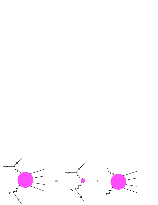
Figure 3: Decomposition of the phase space for the process $e^{+}e^{-}\to e^{+}e^{-}+$ hadrons.

From Eqs. (2.19) and (2.21), we see that both terms in the right-hand side of Eq. (2.18) have a Lorentz-invariant expression. We exploit it to re-write Eq. (2.21) in the center-of-mass frame of the incoming $e^{+}e^{-}$ pair,

$${\rm d}\Gamma=\frac{1}{4(2\pi)^{6}S}\,{\rm d}Q_{1}^{2}\,{\rm d}Q_{2}^{2}\,{\rm d}E_{1}\,{\rm d}E_{2}\,{\rm d}\varphi\,{\rm d}\bar{\varphi},$$ (2.22)

where $\varphi$ and $\bar{\varphi}$ are two generic azimuthal angles, one of which, say $\varphi$ to be definite, can be interpreted as the angle between the two outgoing leptons; $E_{i}$ are the energies of the outgoing leptons in the center-of-mass frame of the incoming $e^{+}e^{-}$ pair. The strategy of the computation should now be clear: although we compute the cross section for the process in Eq. (1.4), the hard process we deal with at NLO is effectively that of Eq. (1.1). Thanks to the decomposition in Eq. (2.18), we have a $2\to n$ phase space which is formally identical to that one gets as a starting point of any NLO algorithm. Thus, we can safely adopt one of the existing NLO algorithms, and study the process of Eq. (1.1) in the $\gamma^{*}\gamma^{*}$ center-of-mass frame, without any reference to the incoming or outgoing leptons. This amounts to a non-trivial simplification, since the complexity of the numerical computations at NLO is known to grow rapidly with the number of particles involved in the hard scattering. Of course, the information on the lepton momenta is entering somewhere, in particular in the matrix elements; to take this fact into account, we proceed in two steps, still using Fig. 3 as a guide. We start by generating the full kinematical configuration of the outgoing leptons, using Eq. (2.22). In doing this, we also get the photon momenta, and therefore we know how to boost from the $e^{+}e^{-}$ to the $\gamma^{*}\gamma^{*}$ center-of-mass frame. Then, we boost the lepton momenta to the $\gamma^{*}\gamma^{*}$ center-of-mass frame, where we generate the remaining (parton) momenta, according to the phase space ${\rm d}{\cal P}_{n}$; at this stage, we can perform all the manipulations required by the NLO algorithm. More details on the final-state kinematics, including bounds on the phase-space variables, can be found in Appendix A.

Following the procedure outlined above, we constructed a code capable of predicting, to NLO accuracy, any infrared-safe quantity constructed with up to three partons (plus two leptons) in the final state. We stress that the code is not of a parton-shower type, and should actually be regarded as a Monte Carlo integrator; however, exactly like in the case of parton-shower Monte Carlo event generators, it allows us to easily implement realistic experimental cuts and to obtain binned differential distributions for all sorts of variables and jet definitions. The code is based upon the NLO algorithm of refs. [36, 37], and it is a suitable modification of one of the codes presented in Ref. [37]. A few technicalities concerning the code are given in Appendix A.

3 Results

In this section, we present results of phenomenological relevance obtained with the code mentioned above. Before assessing the effect of the NLO corrections and comparing our predictions to data, we discuss the choice of the scales entering the electromagnetic and the strong running couplings which appear in the amplitudes. Although arguments exist on the choice of an “optimal” scale, there is no rigorous theorem that prescribes such a choice. Thus, we shall choose the reference scale on the ground of some physical motivations; we stress, however, that alternative choices are possible, and we shall explore a few of them.

3.1 Scale choices

As far as $\alpha_{\rm em}$ is concerned, we have made the choice of evolving it on an event-by-event basis to the scales set by the virtualities of the exchanged photons; hence, we replace the Thomson value $\alpha_{0}\simeq 1/137$ by $\alpha_{\rm em}(Q_{i}^{2})$. This choice better describes the effective strength at which the electromagnetic interaction takes place. Notice that we treat independently the two photon legs: thus, in the formulae relevant to the cross sections, $\alpha_{\rm em}^{4}$ has to be understood as $\alpha_{\rm em}^{2}(Q_{1}^{2})\alpha_{\rm em}^{2}(Q_{2}^{2})$.

An analysis of the differential distributions reveals that, for a typical experimental set-up used at LEP2, defined more precisely below, the mean $Q^{2}$ values fall in the 14–17 GeV² range. At this scale the strength of the electromagnetic interaction is increased by about 3% with respect to the Thomson value. Since $\alpha_{\rm em}$ enters at the fourth power in our squared matrix elements, the 3 % increase in $\alpha_{\rm em}$ translates into an increase of more than 10% in the cross section. Some uncertainty is of course implicit in this number: both the scheme for $\alpha_{\rm em}$ evolution (we used one-loop $\overline{\rm MS}$ running) and the precise scale value will affect the final result by a few per cent.

A similar problem is faced when considering the strong coupling $\alpha_{\scriptscriptstyle S}$, and it is solved in the same way: we define a default scale $\mu_{0}$ so as to match the order of magnitude of the (inverse of the) interaction range:

$$\mu_{0}^{2}=\frac{Q_{1}^{2}+Q_{2}^{2}}{2}+\left(\frac{k_{1{\scriptscriptstyle T}}+k_{2{\scriptscriptstyle T}}+k_{3{\scriptscriptstyle T}}}{2}\right)^{2}\>.$$ (3.1)

The renormalization scale $\mu$ entering $\alpha_{\scriptscriptstyle S}$ will eventually be set equal to $\mu_{0}$ as a default value, and equal to $\mu_{0}/2$ or $2\mu_{0}$ when studying the scale dependence of the cross section. In Eq. (3.1), the $k_{i{\scriptscriptstyle T}}$ are the transverse energies of the outgoing quarks and, for three-particle events, the emitted gluon. Since the hard process is initiated by the two virtual photons, the proper frame to study its properties is the $\gamma^{*}\gamma^{*}$ center-of-mass one. Therefore, when talking about transverse energies, whether in a total cross section or in a jet reconstruction algorithm, this frame will be always understood. This is in fact quite similar to what happens in DIS, where the Breit frame is used. Finally, we point out that the term in parentheses in Eq. (3.1) is, event-by-event, half of the total transverse energy, which is a measurable quantity; at LO, it coincides with the transverse energy of the jets, in the case in which a jet cross section is considered.

We evolve $\alpha_{\scriptscriptstyle S}$ to next-to-leading log accuracy, with $\alpha_{\scriptscriptstyle S}(M_{\scriptscriptstyle Z})=0.1181$ [38] (in $\overline{{\rm MS}}$ at two loops and with five flavours, this implies $\Lambda_{\overline{{\rm MS}}}^{(5)}=0.2275$ GeV).

We also considered a different choice with respect to that in Eq. (3.1); namely, we used $\sqrt{Q_{1}^{2}Q_{2}^{2}}$ instead of $(Q_{1}^{2}+Q_{2}^{2})/2$ in Eq. (3.1). Only very minor differences (much smaller than 1%, i.e., not noticeable on the scale of the plots shown in what follows) were found. This is easily understood since the two scales coincide when $Q_{1}^{2}=Q_{2}^{2}$, and, as we verified explicitly both at the LO and at the NLO, the dominant contribution to the cross section is just due to the region where the virtualities of the two photons are approximately equal.

A third possible choice for the default scale is

$$\bar{\mu}_{0}^{2}=\frac{Q_{1}^{2}+Q_{2}^{2}}{2}\,.$$ (3.2)

Strictly speaking, $\bar{\mu}_{0}$ is arguably better than $\mu_{0}$ when studying fully inclusive quantities, while $\mu_{0}$ is clearly recommended when, for examples, jets are reconstructed. Still, having a tool such as an event generator, we stick to $\mu_{0}$ as our default choice also for fully inclusive observables. However, we also studied the effect of setting $\mu=\bar{\mu}_{0}$, and found only minor differences (of order of 1%) at the level of total cross sections. We shall comment further on the use of $\bar{\mu}_{0}$ in Sect. 3.3.

3.2 Numerical results

We compared our LO result, obtained with fixed $\alpha_{\rm em}=\alpha_{0}$, to the massless limit of the JAMVG program of Ref. [23], and found perfect agreement.

To study the effect of the NLO corrections, we used the experimental cuts employed by the L3 Collaboration; any other physically sensible sets of cuts would lead to the same qualitative conclusions. The scattered electron and positron are required to have energy $E_{1,2}$ larger than 30 GeV and scattering angle $\theta_{1,2}$ between 30 and 66 mrad. Furthermore, the variable $Y$, defined by

$$Y=\log\frac{y_{1}y_{2}S}{\sqrt{Q_{1}^{2}Q_{2}^{2}}}\equiv\log\frac{S}{S_{0}},$$ (3.3)

is required to lie between 2 and 7 ($y_{i}$ are defined in Appendix A, where a discussion on the properties of $Y$ can also be found). The cross sections have been evaluated at $\sqrt{S}=200$ GeV, including up to five massless flavours.

LO, fixed $\alpha_{\rm em}=\alpha_{0}$	LO, running $\alpha_{\rm em}(Q^{2})$	NLO, running $\alpha_{\rm em}(Q^{2})$
0.466	0.534	0.569${}^{+0.006}_{-0.004}$

Table 1: Total cross section (in picobarns) within the L3 experimental cuts at LEP2 energy. The errors in the NLO column refer to the variation of the renormalization scale in the ($\mu_{0}/2,2\mu_{0}$) range.

Within this set of cuts, the replacement of the Thomson electromagnetic coupling $\alpha_{0}$ with the running one is found to increase our LO cross section by about 14% (see Table 1), in agreement with the estimate given above. Such a non-negligible effect should of course be included when comparing to experimental data. Unless stated otherwise, all cross sections considered below will be calculated with the running $\alpha_{\rm em}$.

Table 1 also shows the effect of including the NLO corrections calculated in this paper. They increase the LO total cross section within the cuts applied by about 7 per cent. This increase is of similar size as the $\alpha_{\scriptscriptstyle S}/\pi$ NLO correction to the total hadronic cross section in electron-positron annihilation. The numbers quoted as errors affecting the NLO result are the differences between the cross sections obtained by choosing $\mu=\mu_{0}/2,2\mu_{0}$, and the cross section obtained by using the default value, $\mu=\mu_{0}$. Thus, they should not be interpreted as statistical errors affecting our prediction, but rather as an indication of the theoretical uncertainties due to the scale choice.

Figure 4: Differential cross sections within the L3 experimental cuts at LEP2 energy. Shown are the LO prediction (dashed line) and the NLO ones corresponding to three different choices for the renormalization scale $\mu$.

A better grasp on the effect of the radiative corrections can of course be obtained by studying various differential distributions. Figure 4 shows such distributions for various observables of experimental interest: the energy of the outgoing electron $E_{e^{-}}(\equiv E_{1})$, the hadronic invariant mass $W$, the photon virtuality $Q_{1}^{2}$, and $Y$ as defined in Eq. (3.3). In each plot the leading order curve and the three next-to-leading order ones referring to the three choices ($\mu_{0}/2,\mu_{0},2\mu_{0}$) of the renormalization scale $\mu$ are presented.

The uncertainty related to $\mu$ can be seen to be always smaller than the net effect of including the NLO corrections. It is actually quite difficult to distinguish between the three NLO results (except in the large-$W$ and $Y$ regions), the relative difference between them being of about 1% or less for the total cross section. This also implies that the shape of the distribution is basically independent of $\mu$.

As for the effect of the NLO corrections themselves, we see that, apart from slightly increasing the cross section, they induce visible shape modifications in at least two cases: both the $W$ and the $Y$ distributions become harder after the inclusion of radiative corrections, their effect changing from almost nil at the left edge of the plots to a more than 50% increase at the right one.

Using similar experimental cuts we can also analyse the effect of radiative corrections on jet distributions. We define the jets by means of a $k_{\scriptscriptstyle T}$ clustering algorithm [39], in the version formulated in Ref. [40]. We set the jet-resolution parameter $D=1$ (see Ref. [40]). Contrary to the cuts previously used, here we do not impose an upper limit on $Y$, only requiring $Y>2$. We consider single-inclusive jet and dijet cross sections. In the latter case, we select the jets by imposing a $E_{\scriptscriptstyle T}>14$ GeV cut on the transverse energy of the most energetic jet and requiring $E_{\scriptscriptstyle T}>10$ GeV for at least another jet. We adopt different transverse energy cuts on the two tagged jets in order to avoid the problems that arise in the case in which such cuts are chosen to be equal, as discussed in some details in Ref. [41]. Furthermore, as already mentioned in the Introduction, in the case in which three jets are present in the event, we take as tagged jets the two separated by the largest rapidity interval. Finally, we shall only present results obtained with $\mu=\mu_{0}$.

Figure 5: Differential distributions in jet events: transverse energy in single-inclusive jet production (left panel), and rapidity difference between the most forward/backward jets (right panel) in dijet production.

In the left panel of Fig. 5 we show the transverse energy distribution of single-inclusive jets, considering the cuts $Y>2$ and $Y>6$. The first striking feature of this observable is that the curves relevant to $Y>2$ and $Y>6$ coincide for $E_{\scriptscriptstyle T}>40$ GeV. This is so for the following reason: at the threshold (where the jets are produced at zero rapidity), $W^{2}=4E_{\scriptscriptstyle T}^{2}$; thus using Eq. (A.11) with $E_{\scriptscriptstyle T}=40$ GeV and $Q_{1}^{2}=Q_{2}^{2}=16$ GeV² (which is approximately the average virtuality within the current cuts), we get $Y=5.99$ (here, we identify $Y$ with $\overline{Y}$; see Eq. (A.13)). Therefore, the region $2<Y<6$ simply does not contribute to events with $E_{\scriptscriptstyle T}>40$ GeV. On the other hand, at $E_{\scriptscriptstyle T}=40$ GeV, the two-photon system has just enough energy, at $Y=6$, to produce the jets. Larger values of $Y$ do not contribute much, since the $Y$ spectrum is very rapidly falling at large $Y$’s (see Fig. 4). When considering larger transverse momenta, the situation is exactly the same. We are therefore led to the conclusion that the tail of the $E_{\scriptscriptstyle T}$ spectrum is dominated by threshold production, and therefore cannot be reliably predicted by a fixed-order computation, like ours; a resummation of large threshold logarithms is necessary. A signal that this is indeed the case is reflected in the fact that the radiative corrections are negative in the tail. At smaller transverse energies the behaviour of the radiative corrections displays a pattern similar to that of total rates. For $Y>2$, NLO and LO results are very close to each other; the larger $E_{\scriptscriptstyle T}$, the more important the contributions from threshold production. For $Y>6$, the radiative corrections increase sizably the LO result; this is in agreement with the behaviour of the $Y$ spectrum shown in Fig. 4. The increase is obviously related to the appearance of large logarithms in the cross section, as it is always the case when two scales (here, the small $E_{\scriptscriptstyle T}$ and the large $W$) are present. We shall soon see that the large logarithms in the large-Y region are indeed of BFKL type.

We also considered the transverse energies of the most forward and most backward jet in dijet events, and found a pattern identical to that relevant to single-inclusive jet $E_{\scriptscriptstyle T}$. The reason is clear: even at small transverse energies, three-jet production is clearly disfavoured with respect to dijet production; in the vast majority of the events, there are just two hard jets recoiling against each other.

If we want to study jet production in a sensible way at fixed order, we have therefore to consider observables which are as insensitive as possible to threshold effects. From what we said above, such observables are possibly those that get the dominant contribution from the small-$E_{\scriptscriptstyle T}$ region. An example is given by rapidities. In the right panel of Fig. 5, we show the distributions in the rapidity interval $\Delta\eta$ between the two tagged jets in dijet events, for various cuts on $Y$. In this case, only the NLO results are shown. We have verified that the radiative corrections give positive contributions for all the regions in $Y$ considered, except for $2<Y<4$; in this case, in fact, the energy of the two-photon system is so small that there is no way to get contributions away from the threshold. The most interesting feature of this plot is that it shows that the large-$Y$ and the large-$\Delta\eta$ regions select the same events, as can be inferred from the fact that the distributions relevant to $Y>2$ (solid line) and to $Y>6$ (dot-dashed line) exactly coincide for $\Delta\eta>3.5$. This is actually the same behaviour we observe in the case of the transverse energy distribution, but the underlying physics is rather different. In fact, in this case we also get sizable contributions away from the threshold; thus, at fixed $E_{\scriptscriptstyle T}$, part of the energy of the two-photon system contributes to the longitudinal degrees of freedom, and jets can be produced away from the central region. Since we are in any case dominated by two-jet events, the rapidity difference between the two tagged jets can be easily estimated: $\Delta\eta\simeq\log(W^{2}/E_{T}^{2})$. Therefore, by using Eqs. (A.11) and (A.13), we get $Y\simeq\Delta\eta+\ln(E_{T}^{2}/\sqrt{Q_{1}^{2}Q_{2}^{2}})$. We point out that the pattern displayed in Fig. 5 for large $\Delta\eta$ does not depend upon the transverse momentum cuts: we lowered these cuts down to 5 GeV, and found the same behaviour. The large-$Y$ region is thus naturally suitable to study BFKL physics. In addition, we note that the dijet cross section at NLO is rather small; therefore, with the integrated luminosities at LEP2 a sizeable number of dijet events would hint toward the importance of BFKL-type contributions. Having clarified that the large $Y$ region is basically populated by events characterised by two hard jets well separated in rapidity, we can follow Ref. [22]: we invert Eq. (A.14) to get $c_{\scriptscriptstyle Q}$, substituting $Y=6$ and identifying $L$ with the average $\Delta\eta$ corresponding to the cut $Y>6$ (in this way, we just make a choice for the scale $\mu_{\scriptscriptstyle\rm W}$ entering the BFKL logarithms; other choices are of course possible, and all of them are equally good at the leading logarithm level). We have

$$\log c_{\scriptscriptstyle Q}=Y-\langle\Delta\eta\rangle\simeq 4.32.$$ (3.4)

By inspection of Eq. (A.14), we see that, although $Y$ and the BFKL logarithm $L$ coincide asymptotically, at LEP2 the difference between the two is of the same order of $Y$, and thus cannot be neglected. It seems therefore that LEP2 is quite far from probing the asymptotic BFKL region; it must be stressed, however, that the value given in Eq. (3.4) depends crucially on the assumptions made in Ref. [22].

It is presumed that a BFKL signature from double-tag hadronic events would be observed at an hypothetical Next Linear Collider much more easily than at LEP2. For this to be true, one actually needs fairly small tagging angles, that allow to get relatively small values for the virtualities, with large $W$ values obtainable thanks to the large $e^{+}e^{-}$ center-of-mass energy; in fact, it is argued [21] that it would be desirable to tag the electrons down to 20-40 mrad. We therefore studied the effect of NLO radiative corrections at a NLC with $\sqrt{S}=500$ GeV, requiring $E_{1,2}>40$ GeV, $20<\theta_{1,2}<70$ mrad and $Y>2$; however, we point out that, at present, it seems unlikely that experiments at the NLC will reach such small values for the tagging angles.

The predicted total cross section within these cuts is found to be 0.425 pb at leading order and 0.452 pb at next-to-leading order. The 6% increase is thus similar to the one found at LEP2. The same is true for the $Y$ distribution: for $Y<7$, that is in the range accessible both at LEP2 and at the NLC, the ratio of NLO over LO predictions is to a very good extent the same in the two cases, getting as high as 1.6 at $Y=6$. However, NLC within the cuts given above reaches much larger value in $Y$ ($Y=11$), where the ratio of NLO over LO gets to values of about 2.5. Finally, we verified that the pattern shown in the right panel of Fig. 5 is reproduced also at the NLC: the large-$Y$ and the large-$\Delta\eta$ regions are populated by the same events. Clearly, as in the case of the $Y$ distribution, the values of $\Delta\eta$ accessible at the NLC are larger than at LEP2 (at NLC, $\Delta\eta<7.5$, for transverse energy cuts on jets as given above).

The large NLO corrections that we find in the large-$Y$ region at the NLC show that a calculation of the higher order effects will be necessary in order to sensibly compare the theoretical predictions with the data, and eventually to extract evidence of BFKL dynamics from the latter.

3.3 Comparisons with experimental data at LEP2

$d\sigma/dY$ (pb)        $\sqrt{S}=189-202$ GeV
$\Delta Y$	L3 Data	LO	NLO
2.0 – 2.5	0.50 $\pm$ 0.07 $\pm$ 0.03	0.405	0.396${}^{+0.002}_{-0.002}$
2.5 – 3.5	0.29 $\pm$ 0.03 $\pm$ 0.02	0.213	0.225${}^{+0.001}_{-0.002}$
3.5 – 5.0	0.15 $\pm$ 0.02 $\pm$ 0.01	0.067	0.080${}^{+0.002}_{-0.002}$
5.0 – 7.0	0.08 $\pm$ 0.01 $\pm$ 0.01	0.0091	0.0131${}^{+0.0009}_{-0.0006}$
Total	0.93 $\pm$ 0.05 $\pm$ 0.07	0.534	0.569${}^{+0.006}_{-0.004}$

Table 2: The experimental cross section from L3 compared to leading and next-to-leading order predictions. The uncertainties in the NLO column are related to variations of the renormalization scale.

The L3 [25, 27, 28] and OPAL [26, 29] Collaborations have recently analysed data for hadron production in $\gamma^{*}\gamma^{*}$ collisions at an electron-positron center-of-mass energy around 200 GeV. In this Section, we aim at comparing these data to our NLO results. We remind the reader that our predictions are all given at the parton level, as compared to the data that are of course at the hadron level.

L3 made use of the previously mentioned set of experimental cuts. The cross section they find, as a function of $Y$, is reported in Table 2 and plotted in Fig. 6. Table 2 shows, in four different $Y$ bins, the experimental cross section compared to our leading and next-to-leading order predictions, evaluated at $\sqrt{S}=200$ GeV. The same comparison is made in Fig. 6: the data lie above the theory in the low-$Y$ region, and sizably overshoot the predictions in the large-$Y$ one. Thus we find a marked difference in shape between theory and data which, if confirmed, could be interpreted as the onset of important higher order effects, perhaps of BFKL type. As can be seen from Table 2, the scale uncertainties affecting our predictions are much smaller than the experimental errors; in what follows, we shall therefore refrain from varying the renormalization scale, setting it always equal to its default value $\mu_{0}$. Also, the total cross section does tend to be higher than the predictions, as shown in Table 2. We remind the reader (see Table 1) that the running of the electromagnetic coupling and the inclusion of the NLO corrections have raised the theoretical result from the 0.466 pb given by the massless leading order parton model with $\alpha_{\rm em}=\alpha_{0}$.

Figure 6: Differential cross section with respect to $Y$ from the L3 Collaboration compared to leading and next-to-leading order predictions. The data are taken at $\sqrt{S}=189-202$ GeV. The theoretical simulation is always run at $\sqrt{S}=200$ GeV.

We also compared L3 data of Table 2 to the predictions obtained by choosing $\bar{\mu}_{0}$ as a reference scale (see Eq. (3.2)). As remarked before, the effect on the total cross section is rather small; however, our NLO predictions for the two largest-$Y$ bins in Table 2 get increased by about 6% and 15% respectively. We are thus getting closer to data, but still a very clear disagreement is seen between theory and experiment.

We have also studied the effect of the finite mass of the outgoing heavy quarks in the charm and bottom case, by comparing our results with the ones obtained with the JAMVG [23] code. Within the L3 set of cuts, such mass effects can be seen to decrease the LO massless cross section by an amount of the order of 10-15%. One could in principle rescale the NLO result by this amount and get a phenomenologically sensible prediction but, due to the lack of rigorousness of this procedure, we shall always present our plots and numerical results without such a correction.

The OPAL Collaboration has also recently presented data [29] taken at $\sqrt{S}=189$ - 202 GeV, making use of a slightly different set of cuts: the tagged electron and positron were required to have energies $E_{1,2}>0.4E_{beam}$ and angles $34<\theta_{1,2}<55$ mrad. No cut on $Y$ is applied, but the hadronic invariant mass $W$ is required to be larger than 5 GeV. Our simulation is run within these cuts at an $e^{+}e^{-}$ center-of-mass energy corresponding to the luminosity-weighted average energy of the OPAL data, i.e. $\sqrt{S}=194$ GeV.

$d\sigma/d\overline{Y}$ (pb)        $\sqrt{S}=189$ - 202 GeV
$\Delta\overline{Y}$	OPAL Data	LO	NLO
0 – 1	0.055 $\pm$ 0.016 ${}^{+0.030}_{-0.020}$	0.068	0.062
1 – 2	0.118 $\pm$ 0.024 ${}^{+0.009}_{-0.024}$	0.140	0.133
2 – 3	0.123 $\pm$ 0.028 ${}^{+0.010}_{-0.011}$	0.090	0.093
3 – 4	0.070 $\pm$ 0.021 ${}^{+0.006}_{-0.015}$	0.043	0.049
4 – 6	0.028 $\pm$ 0.013 ${}^{+0.002}_{-0.012}$	0.011	0.014
Total	0.40 $\pm$ 0.05 $\pm$ 0.05	0.364	0.365

Table 3: The experimental cross section from OPAL, total and differential in $\overline{Y}$, compared to leading and next-to-leading order predictions.

Table 3 compares the experimental results obtained with these cuts with our LO and NLO predictions. We can see the NLO corrections to be extremely small. The prediction for the total cross section falls short of the central OPAL result, but is well within the experimental error. Also shown in the same table is the differential distribution in the variable $\overline{Y}$, defined in Eq. (A.11), where a generally good agreement within errors can be observed. Given the large discrepancy between theory and L3 data for this very same variable, it shall therefore be of utmost importance to measure as accurately as possible the $Y$ spectrum, in order to perform a precise study of effects beyond NLO (such as BFKL dynamics).

Figure 7: Differential cross sections within the OPAL experimental cuts ($E_{1,2}>0.4E_{beam}$, $34<\theta_{1,2}<55$ mrad, $W>5$ GeV) at $\sqrt{S}=189-202$ GeV. Shown are the LO prediction (dashed line) and the NLO one (solid). We defined [29] $Q^{2}=\max(Q_{1}^{2},Q_{2}^{2})$, and $x=Q^{2}/(Q_{1}^{2}+Q_{2}^{2}+W^{2})$. $\Delta\phi$ is the difference in azimuthal angle of the outgoing electron and positron, measured in the $e^{+}e^{-}$ center-of-mass frame.

In Fig. 7 we compare our predictions to several distributions related to OPAL data. A good agreement can be observed in all the distributions, with the possible exception of the last two points in the large-$W$ region. Where the difference between the NLO and the LO result is somewhat more sizeable, like in the $x$ distribution and in the large-$W$ and large-$\overline{Y}$ regions, the corrections can be seen to change our predictions in such a way that they get closer to data.

4 Conclusions

We have calculated the NLO corrections, of ${\cal O}(\alpha_{\scriptscriptstyle S})$, to the process

$$\begin{array}[]{rcl}e^{+}+e^{-}&\longrightarrow&e^{+}+e^{-}+\underbrace{\gamma^{*}+\gamma^{*}}\\ &&\phantom{e^{+}+e^{-}+\gamma^{*}\>}\>\raisebox{5.59721pt}{\hbox to0.0pt{$|$\hss}}\!\longrightarrow{\rm hadrons},\end{array}$$ (4.1)

and implemented them into a Monte Carlo integrator which allows the calculation of both total cross sections and differential distributions. We have found the uncertainty related to the choice of renormalization scale to be always smaller than the net effect of including the NLO corrections. This means that the difference between the data and the theoretical predictions of non-BFKL origin, which is the relevant quantity in any attempt to pin down signals of BFKL physics, can now be reliably computed at ${\cal O}(\alpha_{\scriptscriptstyle S})$.

When typical experimental cuts used at LEP2 by the L3 and OPAL Collaborations are applied, NLO corrections to the total cross section are found to be fairly small. Larger effects can instead be observed in the differential distributions, especially in the regions of large $Y$ or large hadronic invariant mass $W$, where the NLO corrections are found to increase the cross section by as much as 50%. No mass effects for final-state charm and bottom quarks have been included. We recall that we have found them to decrease the LO cross section by 10-15% within the set of cuts we have examined, thus worsening the agreement between theory and data.

When comparing to experimental results, we find good agreement with the data measured by the OPAL Collaboration, both at the level of total cross section and differential distributions in a number of different observables. In this case, the effect of NLO corrections is marginal, although the full-NLO curves are seen to be closer to data with respect to the LO predictions: however, this comparison will become more significant only if the errors on data will be substantially reduced. Less good an agreement has instead been found when comparing to L3 data, the NLO predictions tending to fall short of the experimental result. In particular, when comparing with the $Y$ distribution, we can see the data to be sensibly higher than the theoretical prediction in the large-$Y$ region.

The comparison between theory and data at large $Y$’s is of course crucial, since a failure of fixed-order perturbative computations in describing the data in such a region could of course be related to the onset of BFKL-like effects. In this sense, no clear indication can be obtained from our study. If we subtract from L3 and OPAL data at large $Y$’s our ${\cal O}(\alpha_{\scriptscriptstyle S})$ predictions, we get large numbers in both cases (compared to, say, the ${\cal O}(\alpha_{\scriptscriptstyle S})$ results). However, while in the case of L3 these numbers are not statistically compatible with zero, in the case of OPAL they are statistically compatible with zero. Thus, in order to reach a firm conclusion on this matter, the collection of larger statistics is unavoidable. On the other hand, if we take the data at their face value, there is probably an evidence of an effect beyond NLO. It is in our opinion premature to interpret this fact in terms of BFKL physics. The computation of the complete ${\cal O}(\alpha_{\scriptscriptstyle S}^{2})$ rates would be very useful in order to understand this issue.

Appendix A Kinematics

In this Appendix, we collect few useful formulae relevant to the kinematics of the process we study. We define

$$z_{i}={2E_{i}\over\sqrt{S}}\,,\qquad\zeta_{i}={Q_{i}^{2}\over S}\equiv{-q_{i}^{2}\over S}\,,$$ (A.1)

with $\sqrt{S}/2$ the energy of the incoming leptons in their center-of-mass frame. From Eq. (2.22) we thus get

$${\rm d}\Gamma(p_{\ell_{1}},p_{\ell_{2}})={S^{2}\over 16(2\pi)^{6}}\,{\rm d}\zeta_{1}\,{\rm d}\zeta_{2}\,{\rm d}z_{1}\,{\rm d}z_{2}\,{\rm d}\varphi\,{\rm d}\bar{\varphi}\,.$$ (A.2)

The azimuthal angles $\varphi$ and $\bar{\varphi}$ have to be taken in the range $(0,2\pi)$, and it is easy to show that

$$0\leq\zeta_{i}\leq z_{i}\leq 1,\;\;\;\;\;\;i=1,2\,.$$ (A.3)

Using the variables defined in Eq. (A.1), we also get

$$w^{2}(\zeta_{1},\zeta_{2},z_{1},z_{2},\varphi)=(1-z_{1})(1-z_{2})+2\zeta_{1}\zeta_{2}-z_{1}\zeta_{2}-z_{2}\zeta_{1}$$

$$\qquad\qquad\qquad\qquad\;+\,2\cos\varphi\sqrt{\zeta_{1}\zeta_{2}(z_{1}-\zeta_{1})(z_{2}-\zeta_{2})}\,,$$ (A.4)

where $w^{2}=W^{2}/S$ is the scaled squared energy of the $\gamma^{*}\gamma^{*}$ system. The requirement that $w^{2}>0$ further constrains $\zeta_{i}$, $z_{i}$, and $\varphi$.

In real experimental situations the leptonic phase space is severely restricted. The scattered leptons are observed in the forward calorimeters, so the scattering angles $\theta_{i}$ off the beam direction are confined to a small region,

$$\theta_{\rm min}\leq\theta_{i}\leq\theta_{\rm max}\,,\qquad i=1,2\,.$$ (A.5)

We assumed implicitly both in Eq. (A.4) and (A.5) that the $z$ axis is aligned with the incoming electron and the scattering angle of the electron is $\theta_{1}$, while that of the positron is $\theta_{2}+\pi$. Typically $\theta_{\rm min}$ and $\theta_{\rm max}$ are of ${\cal O}$(10 mrad). Furthermore, the energies of the scattered leptons are required to be larger than a certain $E_{\ell}^{\rm min}$ in the $e^{+}e^{-}$ center-of-mass frame. In general, $E_{\ell}^{\rm min}={\cal O}$(10 GeV) at LEP2 energies. In terms of the integration variables, these phase space cuts read as

$${2E_{\ell}^{\rm min}\over\sqrt{S}}{1-\cos\theta_{\rm min}\over 2}\leq\zeta_{i}\leq{1-\cos\theta_{\rm max}\over 2}\,,$$ (A.6)

and $z_{\rm min}\leq z_{i}\leq z_{\rm max}$, where

$$z_{\rm min}={2\zeta_{i}\over 1-\cos\theta_{\rm max}}\,,\qquad z_{\rm max}=\min\left(1,{2\zeta_{i}\over 1-\cos\theta_{\rm min}}\right)\,.$$ (A.7)

In the $e^{+}e^{-}$ center-of-mass frame, we can also use the lepton variables in order to express the photon virtualities

$$-q_{i}^{2}\equiv Q_{i}^{2}=\sqrt{S}E_{i}\left(1-\cos\theta_{i}\right),$$ (A.8)

and the variables $y_{i}$, proportional to the light-cone momentum fraction of the virtual photon

$$y_{i}={q_{i}^{0}+q_{i}^{3}\over\sqrt{S}}=1-{2E_{i}\over\sqrt{S}}\cos^{2}{\theta_{i}\over 2}\,.$$ (A.9)

We also define (see Eq.(3.3))

$$Y=\log\frac{y_{1}y_{2}S}{\sqrt{Q_{1}^{2}Q_{2}^{2}}},$$ (A.10)

and

$$\overline{Y}=\log\frac{W^{2}}{\sqrt{Q_{1}^{2}Q_{2}^{2}}}.$$ (A.11)

The variable $Y$ can also be conveniently expressed in terms of the scaled variables defined in Eq. (A.1):

$$Y=\ln\frac{1-z_{1}+\zeta_{1}}{\sqrt{\zeta_{1}}}+\ln\frac{1-z_{2}+\zeta_{2}}{\sqrt{\zeta_{2}}}\>.$$ (A.12)

$Y$ and $\overline{Y}$ are directly related to the BFKL logarithm $L$ entering Eq. (1.3). In fact, for large $W$’s the $y_{i}$ can be effectively interpreted as the longitudinal momentum fractions of the photons in the incoming leptons (since the transverse components of the photon momenta are much smaller than their larger light-cone component), and thus $W^{2}\simeq y_{1}y_{2}S$, which implies

$$Y\,\stackrel{{\scriptstyle W\to\infty}}{{\longrightarrow}}\,\overline{Y}.$$ (A.13)

Furthermore (see for example Ref. [22]), a sensible choice for the mass scale is $\mu_{\scriptscriptstyle\rm W}^{2}=c_{\scriptscriptstyle Q}\sqrt{Q_{1}^{2}Q_{2}^{2}}$, with $c_{\scriptscriptstyle Q}$ a suitable constant. It then follows that

$$L=\overline{Y}-\log c_{\scriptscriptstyle Q}.$$ (A.14)

Finally, we come back to the issue of the construction of the computer code we used to produce the phenomenological results shown in this paper. The general strategy has been outlined in Sect. 2.3. As discussed there, the NLO algorithm effectively deals with the $2\to 2$ process $\gamma^{*}\gamma^{*}\to q\bar{q}$ (at the tree level and at one loop), and with the $2\to 3$ process $\gamma^{*}\gamma^{*}\to q\bar{q}g$ (at the tree level). We have to stress two important differences due to the off-shellness of the incoming particles ($q_{i}^{2}\neq 0$) with respect to the case described in Refs. [36, 37]. Firstly, in all the formulae given in the appendices of Ref. [37], $S$ has to be substituted with $W^{2}$ (the reader is urged to avoid any confusion between the $S$ of Ref. [37], where $S$ is the center-of-mass energy squared of the partonic system, and the $S$ used in the rest of the present paper). Secondly, the initial-state collinear divergences are absent. Technically, we take this fact into account in the following way: in Eq. (A.1) and (A.15) of Ref. [37], the terms $d\sigma_{a_{1}a_{2},i}^{(in,f)}$ and $d\sigma_{a_{1}a_{2}}^{(1,N-1r)}$ are set to zero. Accordingly, there is no need to introduce ${\cal P}_{i}^{(0)}$ in the decomposition of the ${\cal P}$ functions (see Eq. (3.10) of Ref. [37]), and only ${\cal P}_{ij}^{(1)}$ is non vanishing. Notice that, since now the regions of the phase space where one of the final-state partons is collinear to one of the initial-state particles are not infrared singular, the functions ${\cal P}_{ij}^{(1)}$ do not need to vanish in these regions. In order to construct the code relevant to the present paper, we implemented what discussed above in the hadronic code of Ref. [37]. On top of that, the generation of the momenta of the leptons has been added, as discussed in Sect. 2.3. The matrix elements were coded as described in Sect. 2.1 and 2.2.

Appendix B Notation for helicity amplitudes

In order to evaluate the production rates in Sect. 2.1, we use helicity amplitudes, defined in terms of massless Dirac spinors $\psi_{\pm}(p)$ of fixed helicity,

$$\psi_{\pm}(p)={1\pm\gamma_{5}\over 2}\psi(p)\equiv|p^{\pm}\rangle\,,\qquad\overline{\psi_{\pm}(p)}\equiv\langle p^{\pm}|\,,$$ (B.1)

spinor products,

$$\langle pk\rangle\equiv\langle p^{-}|k^{+}\rangle\,,\qquad\left[pk\right]\equiv\langle p^{+}|k^{-}\rangle\,,$$ (B.2)

currents,

$$\langle i|k|j\rangle \equiv \langle i^{-}|/\!\!\!k|j^{-}\rangle=\langle ik\rangle\left[kj\right]\,,$$

$$\langle i|(k+l)|j\rangle \equiv \langle i^{-}|(/\!\!\!k+/\!\!\!l)|j^{-}\rangle$$ (B.3)

and Mandelstam invariants

$$s_{pk}=2p\cdot k=\langle pk\rangle\left[kp\right]\,,\qquad t_{pkq}=(p+k+q)^{2}\,.$$ (B.4)

References

- [1] S. Aid et al. [H1 Collaboration], Phys. Lett. B354 (1995) 494 [hep-ex/9506001].
- [2] S. Forte and R. D. Ball, hep-ph/9607291.
- [3] S. Aid et al. [H1 Collaboration], Phys. Lett. B356 (1995) 118 [hep-ex/9506012].
- [4] J. Breitweg et al. [ZEUS Collaboration], Eur. Phys. J. C6 (1999) 239 [hep-ex/9805016].
- [5] C. Adloff et al. [H1 Collaboration], Nucl. Phys. B538 (1999) 3 [hep-ex/9809028].
- [6] J. Bartels, V. Del Duca, A. De Roeck, D. Graudenz and M. Wusthoff, Phys. Lett. B384 (1996) 300 [hep-ph/9604272].
- [7] L. H. Orr and W. J. Stirling, hep-ph/9804431.
- [8] S. Abachi et al. [D0 Collaboration], Phys. Rev. Lett. 77 (1996) 595 [hep-ex/9603010].
- [9] B. Abbott et al. [D0 Collaboration], Phys. Rev. Lett. 84 (2000) 5722 [hep-ex/9912032].
- [10] A. H. Mueller and H. Navelet, Nucl. Phys. B282 (1987) 727.
- [11] V. Del Duca and C. R. Schmidt, Phys. Rev. D49 (1994) 4510 [hep-ph/9311290].
- [12] W. J. Stirling, Nucl. Phys. B423 (1994) 56 [hep-ph/9401266].
- [13] V. Del Duca and C. R. Schmidt, Phys. Rev. D51 (1995) 2150 [hep-ph/9407359].
- [14] L. H. Orr and W. J. Stirling, Phys. Lett. B429 (1998) 135 [hep-ph/9801304].
- [15] E. A. Kuraev, L. N. Lipatov and V. S. Fadin, Sov. Phys. JETP 44 (1976) 443.
- [16] E. A. Kuraev, L. N. Lipatov and V. S. Fadin, Sov. Phys. JETP 45 (1977) 199.
- [17] I. I. Balitsky and L. N. Lipatov, Sov. J. Nucl. Phys. 28 (1978) 822.
- [18] E. Mirkes and D. Zeppenfeld, Phys. Rev. Lett. 78 (1997) 428 [hep-ph/9609231].
- [19] A. H. Mueller, Nucl. Phys. B415 (1994) 373.
- [20] A. H. Mueller and B. Patel, Nucl. Phys. B425 (1994) 471 [hep-ph/9403256].
- [21] J. Bartels, A. De Roeck and H. Lotter, Phys. Lett. B389 (1996) 742 [hep-ph/9608401].
- [22] S. J. Brodsky, F. Hautmann and D. E. Soper, Phys. Rev. D56 (1997) 6957 [hep-ph/9706427].
- [23] J. A. Vermaseren, Nucl. Phys. B229 (1983) 347.
- [24] J. F. Gunion and Z. Kunszt, Phys. Rev. D33 (1986) 665.
- [25] M. Acciarri et al. [L3 Collaboration], Phys. Lett. B453 (1999) 333.
- [26] OPAL Collaboration, OPAL Physics Note PN-391.
- [27] L3 Collaboration, L3 Note 2568, presented at ICHEP 2000, Osaka, Japan.
- [28] M. Wadhwa, for the L3 Collaboration, presented at Photon 2000, Ambleside, UK.
- [29] OPAL Collaboration, OPAL Physics Note PN456.
- [30] L. Dixon, Z. Kunszt and A. Signer, Nucl. Phys. B531 (1998) 3 [hep-ph/9803250].
- [31] Z. Bern, L. Dixon and D. A. Kosower, Nucl. Phys. B513 (1998) 3 [hep-ph/9708239].
- [32] W. Siegel, Phys. Lett. B84 (1979) 193.
- [33] D. M. Capper, D. R. Jones and P. van Nieuwenhuizen, Nucl. Phys. B167 (1980) 479.
- [34] Z. Bern and D. A. Kosower, Nucl. Phys. B379 (1992) 451.
- [35] S. Catani, M. H. Seymour and Z. Trócsányi, Phys. Rev. D55 (1997) 6819 [hep-ph/9610553].
- [36] S. Frixione, Z. Kunszt and A. Signer, Nucl. Phys. B467 (1996) 399 [hep-ph/9512328].
- [37] S. Frixione, Nucl. Phys. B507 (1997) 295 [hep-ph/9706545].
- [38] D. E. Groom et al., Eur. Phys. J. C15 (2000) 1.
- [39] S. Catani, Y. L. Dokshitzer, M. H. Seymour and B. R. Webber, Nucl. Phys. B406 (1993) 187.
- [40] S. D. Ellis and D. E. Soper, Phys. Rev. D48 (1993) 3160 [hep-ph/9305266].
- [41] S. Frixione and G. Ridolfi, Nucl. Phys. B507 (1997) 315 [hep-ph/9707345].