TPI-MINN-00/46, UMN-TH-1922-00

McGill-00/31; IASSNS-HEP-00/83

hep-ph/0011335

The Minimal Model of Nonbaryonic Dark Matter:
A Singlet Scalar
C.P. Burgess^a,b, Maxim Pospelov^c and Tonnis ter Veldhuis^c
a The Institute for Advanced Study, Princeton, NJ 08540, USA
^b Physics Department, McGill University,
3600 University St., Montréal, Québec, Canada, H3A 2T8.
^c Department of Physics, University of Minnesota
Minneapolis, MN 55455, USA
Abstract

We propose the simplest possible renormalizable extension of the Standard Model — the addition of just one singlet scalar field — as a minimalist model for non-baryonic dark matter. Such a model is characterized by only three parameters in addition to those already appearing within the Standard Model: a dimensionless self-coupling and a mass for the new scalar, and a dimensionless coupling, $\lambda$, to the Higgs field. If the singlet is the dark matter, these parameters are related to one another by the cosmological abundance constraint, implying that the coupling of the singlet to the Higgs field is large, $\lambda\sim O(0.1-1)$. Since this parameter also controls couplings to ordinary matter, we obtain predictions for the elastic cross section of the singlet with nuclei. The resulting scattering rates are close to current limits from both direct and indirect searches. The existence of the singlet also has implications for current Higgs searches, as it gives a large contribution to the invisible Higgs width for much of parameter space. These scalars can be strongly self-coupled in the cosmologically interesting sense recently proposed by Spergel and Steinhardt, but only for very low masses ($\mathrel{\raise 1.29167pt\hbox{$<$\kern-7.5pt\lower 4.30554pt\hbox{$\sim$}}}1$ GeV), which is possible only at the expense of some fine-tuning of parameters.

1 Introduction

It is an amazing fact of our times that even as our understanding of cosmology progresses by leaps and bounds, we remain almost completely ignorant about the nature of most of the matter in the universe. According to recent fits to cosmological parameters [1], dark matter of some sort makes up close to 30% of the total energy density. This is much more than what is inferred from inventories of the luminous matter we can see. Moreover, the successes of big bang nucleosynthesis suggest that only a fraction of this matter can be made of ordinary baryons, like massive compact objects, faint stars, etc.. Thus, unless gravity undergoes some drastic changes at distances larger than a few kpc (which is quite improbable from several points of view), we must postulate the existence of enormous amounts of dark matter of an unknown, non-baryonic origin.

A simple argument shows why current theories of particle physics are so prolific in suggestions for what the nature of this dark matter might be [2]. The vast majority of the proposed alternatives to the Standard Model involve new particles having masses which are of order $m_{\scriptscriptstyle W}\sim 100$ GeV, and which couple with electroweak strength to the ordinary matter which we know and love. If any of these particles is stable enough to have a lifetime as long as the age of the universe, it makes a natural candidate for dark matter. It does so because its abundance is naturally of the right order of magnitude so long as its interaction cross sections have weak-interaction strength. The abundance comes out right because it is set by the annihilation rate for particles which are initially in thermal equilibrium with ordinary matter. Cosmologically interesting abundances follow pretty much automatically for particles whose mass is of order $m_{\scriptscriptstyle W}$ and whose annihilation cross sections have weak (or rather milliweak) interaction strength. (We give this argument in more detail within the body of the paper.)

Better yet, supersymmetric models, which are perhaps the best motivated of the many theories which have been proposed, very often have such long-lived states, due to the natural existence there of a conserved quantum number, $R$-parity, which keeps the lightest $R$-odd state from decaying. These particles cry out for interpretation as dark-matter particles, and it is no surprise that these models are by far the most widely explored in the literature [3].

Best of all, this explanation of the nature of dark matter can be tested experimentally. This is the direct goal of dedicated dark-matter detectors [4], and an indirect goal of accelerator searches for events with missing energy, showing that a weakly-interacting particle has escaped the detector. If Nature smiles on us we soon may be treated to the discovery of new physics in both of these kinds of experiments. Indeed, recently the DAMA collaboration has announced the detection of a dark matter signal, as indicated by their seeing an annual modulation of the counting rate in a NaI detector [5]. However, the comparably precise data from the Ge detectors of the CDMS collaboration [6] do not support these findings. (These two experiments need not be in contradiction with each other if the spin-dependent part of the cross-section is enhanced relative to the spin-independent part [7].)

Our goal in the present paper is to present a slightly unorthodox view. Although very well motivated, supersymmetric models are very complicated and enjoy an enormous parameter space. This makes them unable to definitively predict what dark-matter detectors must see. Furthermore, unlike the extensive evidence for the existence of dark matter, the arguments in favour of supersymmetry are almost exclusively theoretical. In our opinion, with the advent of good-quality data from dark-matter detectors, it behooves theorists to propose simple models for the dark matter which are consistent with present evidence, but which make definite predictions and so are easily falsifiable. These provide benchmarks against which other models and the data can be compared. We believe that it is only by comparing the implications of such models with one another, and with supersymmetry, that one can hope to properly interpret the data.

The model we study in this paper was first introduced by Veltman and Yndurain [8] in a different context. Its cosmology was later studied by Silveira and Zee [9], and (with a complex scalar) by McDonald [10]. It is the absolute minimal modification of the Standard Model which can explain the dark matter. It consists of the addition of a single spinless species of new particle, $S$, to those of the Standard Model, using only renormalizable interactions. To keep the new particle from interacting too strongly with ordinary matter, it is taken to be completely neutral under the Standard Model gauge group. Besides involving the fewest new states, the model is also just complicated enough to offer interestingly rich dark matter properties. Unlike the case if only spin-half or only spin-one singlet particles are added, it is possible for a singlet scalar to have both significant renormalizable self-interactions and renormalizable interactions with some Standard Model fields.

There is also a sense in which the model we propose is generic, should the dark matter consist of a single species of spinless particle. To this end, it is useful to ask the question of what a generic dark-matter model should look like. It is clear that the main property which one needs to ensure is the stability of the new particle, suggesting that the fields $S_{i}$, representing these particles appears in the Lagrangian in even powers, so that its decay is forbidden. If this field $S_{i}$ is considerably lighter than the rest of the other exotic undiscovered particles, these may be integrated out, leaving an effective Lagrangian at electroweak scale which has the generic form

$${\cal L}={\rm kinetic\leavevmode\nobreak\ term\leavevmode\nobreak\ for}\leavevmode\nobreak\ S_{i}+S_{i}^{*}MS_{i}+\sum S_{i}^{*}O_{\scriptscriptstyle SM}S_{i}+...$$ (1.1)

where the kinetic, mass terms and interactions with the SM (via the set of operators $O_{\scriptscriptstyle SM}$) in general would depend on the spin of $S_{i}$. The most important couplings at low energies are those of lowest dimension, corresponding to the lowest-dimension choices for the operators $O_{\scriptscriptstyle SM}$. Our model also has this form, with only a single singlet scalar $S$. In this language, our dropping of all nonrenormalizable interactions corresponds to keeping only those interactions which are consistent with (but do not require) all other exotic particles to be arbitrarily heavy compared with the weak scale. We might expect our model to therefore capture the physics of any more complicated theory whose impact on the dark matter problem is conveyed purely through the low-energy interactions of a single spinless particle.

An additional, more tentative, incentive for formulating more models stems from recent indications of problems with subgalactic structure formation within the non-interacting cold-dark-matter scenario [11]. A ‘generalized’ form of cold dark matter may avoid these problems if its self-interactions can produce scattering cross sections of order $10^{-24}$ cm² in size [12]. Within the present context this proposal would require the masses of dark matter particles not to exceed 1 GeV. Within the minimal model described in this paper, we find this range of masses may be just barely possible, but requires unnatural fine tunings due to the relationship between masses and couplings imposed by the maintenance of the correct cosmic abundance of dark-matter scalars.

This paper is organized as follows. In the next section we identify the three parameters which describe the model, and determine the general conditions which lead to acceptable masses and to sufficiently stable dark matter. In section 3 we calculate the annihilation cross section of $S$-particles and give the resulting cosmic abundance as a function of masses and couplings. This calculation is similar to the analysis of Ref. [10]. We perform the numerical analysis for the most interesting part of the parameter space, with 100 GeV $\leq m_{h}\leq$ 200 GeV and 10 GeV $\leq m_{\scriptscriptstyle S}\leq$ 100 GeV. In section 4 we obtain the cross section for elastic scattering with ordinary matter and apply the constraints, imposed by direct and indirect searches. Section 5 computes the cross sections for the missing energy events which are predicted for colliders due to the pair production of $S$ particles. It also contains a prediction for the degradation of the Higgs boson signal at hadronic colliders, when the Higgs boson is allowed to decay into a pair of $S$ particles. Our conclusions are reserved for section 6.

2 The Model’s Lagrangian

The lagrangian which describes our model has the following simple form:

$${\cal L}={\cal L}_{\scriptscriptstyle SM}+\frac{1}{2}\partial_{\mu}S\,\partial^{\mu}S-\frac{m_{0}^{2}}{2}\;S^{2}-\frac{\lambda_{\scriptscriptstyle S}}{4}\,S^{4}-\lambda\,S^{2}\,H^{\dagger}H,$$ (2.1)

where $H$ and ${\cal L}_{\scriptscriptstyle SM}$ respectively denote the Standard Model Higgs doublet and lagrangian, and $S$ is a real scalar field which does not transform under the Standard Model gauge group. (Lagrangians similar to this have been considered as models for strongly-interacting dark matter [14] and as potential complications for Higgs searches [15]. The same number of free parameters appears in the simplest Q-ball models [16].) We assume $S$ to be the only new degree of freedom relevant at the electroweak scale, permitting the neglect of nonrenormalizable couplings in eq. (2.1), which contains all possible renormalizable interactions consistent with the field content and the symmetry $S\to-S$.

Within this framework the properties of the field $S$ are described by three parameters. Two of these, $\lambda_{\scriptscriptstyle S}$ and $m_{0}$ are internal to the $S$ sector, characterizing the $S$ mass and the strength of its self-interactions. Of these, $\lambda_{\scriptscriptstyle S}$ is largely unconstrained and can be chosen arbitrarily. We need only assume it to be small enough to permit the perturbative analysis which we present. Couplings to all Standard Model fields are controlled by the single parameter $\lambda$.

We now identify what constraints are implied for these couplings by general considerations like vacuum stability or from the requirement that the vacuum produce an acceptable symmetry-breaking pattern. These are most simply identified in unitary gauge, $\sqrt{2}\,H^{\dagger}=(h,0)$ with real $h$, where the scalar potential takes the form:

$$V=\frac{m_{0}^{2}}{2}\,S^{2}+\frac{\lambda}{2}\;S^{2}h^{2}+\frac{\lambda_{\scriptscriptstyle S}}{4}\,S^{4}+\frac{\lambda_{h}}{4}\Bigl{(}h^{2}-v_{\scriptscriptstyle EW}^{2}\Bigr{)}^{2}.$$ (2.2)

$\lambda_{h}$ and $v_{\scriptscriptstyle EW}=246$ GeV are the usual parameters of the Standard Model Higgs potential.

1. The Existence of a Vacuum: This potential is bounded from below provided that the quartic couplings satisfy the following three conditions:

$$\lambda_{\scriptscriptstyle S},\leavevmode\nobreak\ \lambda_{h} \geq 0$$ and (2.3)

$$\qquad\lambda_{\scriptscriptstyle S}\,\lambda_{h} \geq \lambda^{2}\qquad\hbox{for negative $\lambda$}.$$

We shall assume that these relations are satisified and study the minima of the scalar potential.

2. Desirable Symmetry Breaking Pattern: We demand the minimum of $V$ to have the following two properties: It must spontaneously break the electroweak gauge group, $\langle h\rangle\neq 0$; and it must not break the symmetry $S\to-S$, so $\langle S\rangle=0$. The first of these is an obvious requirement in order to have acceptable particle masses, while the second is necessary in order to ensure the longevity of $S$ in a natural way. ($S$ particles must survive the age of the universe in order to play their proposed present role as dark matter.)

The configuration $h\neq 0$ and $S=0$ is a stationary point of $V$ if and only if $v_{\scriptscriptstyle EW}^{2}>0$, in which case the extremum occurs at $h_{\rm ext}^{2}=v_{\scriptscriptstyle EW}^{2}$. This is a local minimum if and only if

$$m_{0}^{2}+\lambda\,v_{\scriptscriptstyle EW}^{2}>0.$$ (2.4)

A second local minimum, with $h_{\rm ext}=0$ and $S_{\rm ext}^{2}=-m_{0}^{2}/\lambda_{\scriptscriptstyle S}$, can also co-exist with the desired minimum if $\lambda>0$ and $\lambda^{2}<\lambda_{h}\lambda_{\scriptscriptstyle S}$. This second minimum is present so long as $m_{0}^{2}<0$ and $-\lambda m_{0}^{2}>\lambda_{\scriptscriptstyle S}\lambda_{h}v_{\scriptscriptstyle EW}^{2}$. Even in this case, the minimum at $S_{\rm ext}=0$ and $h_{\rm ext}^{2}=v_{\scriptscriptstyle EW}^{2}$ is deeper, and so is the potential’s global minimum, provided that

$$0<-m_{0}^{2}<v_{\scriptscriptstyle EW}^{2}\sqrt{\lambda_{h}\lambda_{\scriptscriptstyle S}}.$$ (2.5)

Throughout the rest of this paper, the above conditions are assumed to hold, so that the model is in a phase having potentially acceptable phenomenology. It is therefore convenient to shift $h$ by its vacuum value, $h\to h+v_{\scriptscriptstyle EW}$, so that $h$ represents the physical Higgs having mass $m_{h}^{2}=\lambda_{h}\,v_{\scriptscriptstyle EW}^{2}$. The $S$-dependent part of the scalar potential then takes its final form

$$V=\frac{1}{2}\,\Bigl{(}m_{0}^{2}+\lambda\,v_{\scriptscriptstyle EW}^{2}\Bigr{)}S^{2}+\frac{\lambda_{\scriptscriptstyle S}}{4}\,S^{4}+\lambda v_{\scriptscriptstyle EW}\,S^{2}\,h+\frac{\lambda}{2}\,S^{2}\,h^{2},$$ (2.6)

and the $S$ mass is seen to be $m_{\scriptscriptstyle S}^{2}=m_{0}^{2}+\lambda v_{\scriptscriptstyle EW}^{2}$. Our prejudice in what follows is that this mass lies in the range from a few to a few hundred GeV, in which case the resulting dark matter will be cold.

3 Constraints from Cosmological Abundance

We next sharpen the cosmological constraints on the model by demanding the present abundance of $S$ particles to be close to today’s preferred value of $\Omega_{\scriptscriptstyle S}h^{2}$. This imposes a strong relationship between the parameters $\lambda$ and $m_{\scriptscriptstyle S}$, which we now derive.

We start by assuming that the $S$ particles are in thermal equilibrium with ordinary matter for temperatures of order $m_{\scriptscriptstyle S}$ and above. This is ensured so long as the coupling $\lambda$ is not too small. Just how small $\lambda$ must be is determined by the following argument. Thermal equilibrium requires the thermalization rate, $\Gamma_{\rm th}$, to be larger than the universal Hubble expansion rate, $H$. The constraint on $\lambda$ comes from the demand that this be true throughout the thermal history of the universe, down to temperatures $T<m_{\scriptscriptstyle S}\sim m_{\scriptscriptstyle W}$. But $\Gamma_{\rm th}$ and $H$ vary differently with time as the universe expands, because they differ in their temperature dependence. On one hand, in the radiation-dominated epoch which is of primary interest to us, $H\sim T^{2}/M_{\rm Pl}$, where $M_{\rm Pl}$ denotes the Planck mass. On the other hand, the thermalization rate varies as $\Gamma_{\rm th}\sim\lambda^{2}T$ for $T\gg m_{h}$, and as $\Gamma_{\rm th}\sim\lambda^{2}T^{5}m_{h}^{-4}$ for $T\ll m_{h}$. These temperature dependences imply the ratio $R_{\rm th}=\Gamma_{\rm th}/H$ is maximized when $T\sim m_{h}\sim m_{\scriptscriptstyle W}$, taking the maximum value $R_{\rm th}\sim\lambda^{2}M_{\rm Pl}/m_{h}$. $S$ particles are therefore guaranteed to remain thermalized (or get thermalized) down to the electroweak epoch, $T\sim m_{h}\sim m_{\scriptscriptstyle W}$, if this maximum ratio is required to be of order one or larger, implying

$$\lambda\mathrel{\raise 1.29167pt\hbox{$>$\kern-7.5pt\lower 4.30554pt\hbox{$\sim$}}}\sqrt{\frac{m_{\scriptscriptstyle W}}{M_{\rm Pl}}}\sim 10^{-8}.$$ (3.1)

Once thermalization is reached (and in the absence of $S$ decays), as we shall henceforth assume, the primordial $S$ abundance is determined by the $S$ particle mass and its annihilation cross section. This cross section depends very strongly on the unknown Higgs mass, and on which annihilation channels are kinematically open.

An independent, interesting issue is the fate of a scalar condensate that might survive from the inflationary epoch. After the Hubble rate drops below $m_{S}$, coherent time oscillations of the singlet field begin. These oscillations can be regarded as the oscillations of a Bose condensate of $S$ particles which is not in thermal equilibrium with other matter. The fate of the condensate depends on the initial value of the $S$ field and two possibilities must be distinguished. If the initial value of the condensate is sufficiently small so that the energy density in the oscillations, $\sim m_{S}^{2}\langle S\rangle^{2}$, is smaller than the energy density of radiation, $\sim T^{4}$, then the thermalization of this condensate occurs exponentially fast. The rate is given by $\lambda^{2}T$ or $\lambda_{S}^{2}T$, whichever is larger. When the initial value of the condensate is of the order of the electroweak v.e.v., the condensate will therefore completely disappear if $\lambda$ or $\lambda_{S}$ is larger then $\sqrt{M_{W}/M_{\rm Pl}}$, just as in the thermalization condition (3.1). The situation is quite different when the initial value of the $S$ field is very large ($M_{\rm Pl}$, for example). The $S$ condensate then dominates the energy density in the Universe and it behaves exactly as the inflaton condensate. The absence of the direct decay of $S$ particles in this case may prevent the universe from reheating [17] . In this paper we assume that $S$ field does not drive inflation, and we limit ourselves to the first possibility.

Figure 1: The Feynman graph relevant to $S$-particle annihilation via Higgs exchange. Various annihilation channels are open or forbidden, depending on the value of $2m_{\scriptscriptstyle S}$.

Since the temperature domain for which annihilation is most important is $T_{\rm ann}\sim 0.05\,m_{\scriptscriptstyle S}$, it is the nonrelativistic annihilation cross section which is relevant. In our model the expression for the annihilation rate depends on which phase within which it occurs. If it occurs within the Higgs phase, i.e. if $T_{\rm ann}$ is low enough so that it occurs after the electroweak phase transition, the result is given by evaluating the tree-level graph of fig. (1) for $s$-channel annihilation, $SS\to X$,which in the nonrelativistic limit gives

$$\sigma_{\rm ann}\;v_{rel} = \frac{8\lambda^{2}v_{\scriptscriptstyle EW}^{2}}{(4m_{\scriptscriptstyle S}^{2}-m_{h}^{2})^{2}+m_{h}^{2}\Gamma_{h}^{2}}\;F_{\scriptscriptstyle X}$$ (3.2)

$$\hbox{with}\qquad F_{\scriptscriptstyle X} := \lim_{m_{\tilde{h}}\to 2m_{\scriptscriptstyle S}}\left(\frac{\Gamma_{\scriptscriptstyle\tilde{h}X}}{m_{\tilde{h}}}\right).$$

Here $\Gamma_{h}$ is the total Higgs decay rate, and $\Gamma_{\scriptscriptstyle\tilde{h}X}$ denotes the partial rate for the decay, $\tilde{h}\to X$, for a virtual Higgs, $\tilde{h}$, whose mass is $m_{\tilde{h}}=2m_{\scriptscriptstyle S}$. Eq. (3.2) also assumes that $m_{\scriptscriptstyle S}<m_{h}$, so that direct (contact) annihilation to a pair of physical Higgses via the $\lambda S^{2}h^{2}$ interaction term is forbidden.

Of particular interest are the large- and small-$m_{\scriptscriptstyle S}$ limits. The small-$m_{\scriptscriptstyle S}$ limit of eq. (3.2) – $m_{\scriptscriptstyle S}\ll m_{\scriptscriptstyle W},\leavevmode\nobreak\ m_{h}$ – implies the asymptotic behaviour:

$$\sigma_{\rm ann}v_{rel}\propto\frac{\lambda^{2}\,m_{\scriptscriptstyle S}^{2}}{m_{h}^{4}}\qquad\hbox{if}\;m_{\scriptscriptstyle S}\ll m_{h},$$ (3.3)

and the coefficient of proportionality depends strongly on the accessibility of certain decay channels ($X=\pi\pi$ or $\mu^{+}\mu^{-}$, and so on).

For large $m_{\scriptscriptstyle S}$ the dominant contributions to the annihilation cross section come from $W^{+}W^{-}$, $ZZ$ and $hh$ final states. (The latter originates from the $\lambda S^{2}h^{2}$ interaction term, whose contribution must be summed with (3.2)). Neglecting terms which are $O(v_{\scriptscriptstyle EW}^{2}/m_{\scriptscriptstyle S}^{2})$ in the result, we find the large-$m_{\scriptscriptstyle S}$ behavior of the annihilation cross section to be

$$\sigma_{\rm ann}v_{rel}\approx\frac{\lambda^{2}}{4\pi m_{\scriptscriptstyle S}^{2}},\qquad\hbox{if}\;m_{\scriptscriptstyle S}\gg m_{h}.$$ (3.4)

These asymptotic forms are useful in what follows for understanding what the cosmological abundance constraint implies for the coupling $\lambda$ in the limit where $m_{\scriptscriptstyle S}$ is very large or very small. Our results for the annihilation cross section agree with the calculation of ref. [10].

Figure 2: Four samples of the $\log\lambda$–$m_{\scriptscriptstyle S}$ relationship between $\lambda$ and $m_{\scriptscriptstyle S}$, which gives the correct cosmic abundance of $S$ scalars. For these plots the Higgs mass is chosen to be 100, 120, 140, and 200 GeV. The abundance is chosen to be $\Omega_{s}h^{2}=0.3$

These expressions may be used with standard results for the Standard Model Higgs decay widths to predict how the primordial $S$-particle abundance depends on the parameters $m_{\scriptscriptstyle S}$ and $\lambda$. Standard procedures [18] give the present density of $S$ particles to be

$$\Omega_{s}h^{2}=\frac{(1.07\cdot 10^{9})\;x_{f}}{g_{*}^{1/2}\leavevmode\nobreak\ M_{\rm Pl}\leavevmode\nobreak\ {\rm GeV}\leavevmode\nobreak\ \langle\sigma v_{\rm rel}\rangle}.$$ (3.5)

Here $g_{*}$, as usual, counts the degrees of freedom in equilibrium at annihilation, $x_{f}=m_{\scriptscriptstyle S}/T_{f}$ is the inverse freeze-out temperature in units of $m_{\scriptscriptstyle S}$, which can be determined by solving the equation $x_{f}\simeq\ln\Bigl{[}0.038(g_{*}x_{f})^{-1/2}M_{\rm Pl}\,m_{\scriptscriptstyle S}\langle\sigma v\rangle\Bigr{]}$. Finally, $\langle\cdots\rangle$ denotes the relevant thermal average.

The abundance constraint is obtained by requiring $\Omega_{s}h^{2}$ to be in the cosmologically preferred range, which imposes a relation between $\lambda$ and $m_{\scriptscriptstyle S}$. For our numerical results we use $\Omega_{s}h^{2}=0.3$, which corresponds to a large value for $\Omega_{s}=0.6$, perhaps the largest possible value consistent with observations. We choose such a large $\Omega_{s}$ in order to be conservative in our later predictions for the signals to be expected in dark matter detectors, since larger $\Omega_{s}$ corresponds to smaller $\lambda$. Choosing instead the central value, $\Omega_{s}h^{2}\simeq 0.15$, obtained from various cosmological fits would give values for $\lambda^{2}$ which are about twice as large as those which we use in what follows. Since it happens that $x_{f}\sim 20$ is approximately constant for the range of cross-sections and masses expected in this model, the abundance condition is equivalent to holding $\langle\sigma v\rangle$ constant as $\lambda$ and $m_{\scriptscriptstyle S}$ are varied (provided $g_{*}$ is held constant).

Fig. (2) plots the relationship between $\lambda$ and $m_{\scriptscriptstyle S}$ which is predicted in this way by the requirement that $\Omega_{s}h^{2}\sim 0.3$. For most values of $m_{\scriptscriptstyle S}$ this curve is well described by the above simple formulae, which give sufficient accuracy in most parts of the parameter space defined by varying $m_{\scriptscriptstyle S}$, $\lambda$ and $m_{h}$. Important exceptions to this statement apply in kinematically special regions, such as the Higgs threshold ($2m_{\scriptscriptstyle S}\simeq m_{h}$) and two-particle thresholds in the final states ($2m_{\scriptscriptstyle S}\simeq 2m_{b}$ or $2m_{\scriptscriptstyle S}\simeq 2m_{\scriptscriptstyle W}$, and so on), where a more sophisticated treatment is required. In our quantitative work we follow the numerical procedure outlined in Ref. [19] in these special regions.

For $m_{\scriptscriptstyle S}$ sufficiently large or small, the asymptotic expressions (3.3) and (3.4) show that the abundance constraint forces $\lambda$ to become large, eventually becoming too large to believe perturbative expressions like eq. (3.2). In particular, if annihilation should occur before the electroweak transition, then the asymptotic relation between $\lambda$ and $m_{\scriptscriptstyle S}$ becomes:

$$\lambda\sim\frac{m_{\scriptscriptstyle S}}{10\leavevmode\nobreak\ {\rm TeV}},$$ (3.6)

so demanding the perturbative regime ($\lambda\mathrel{\raise 1.29167pt\hbox{$<$\kern-7.5pt\lower 4.30554pt\hbox{$\sim$}}}1$) gives the upper bound $m_{\scriptscriptstyle S}\mathrel{\raise 1.29167pt\hbox{$<$\kern-7.5pt\lower 4.30554pt\hbox{$\sim$}}}10$ TeV.

For small $m_{\scriptscriptstyle S}$ we consider the case $m_{\scriptscriptstyle S}=500$ MeV, for which the dominant annihilation channels are $\pi^{+}\pi^{-}$, $\pi^{0}\pi^{0}$ and $\mu^{+}\mu^{-}$ [20]. In this case $\Omega_{s}h^{2}\mathrel{\raise 1.29167pt\hbox{$<$\kern-7.5pt\lower 4.30554pt\hbox{$\sim$}}}0.3$ is achieved if the coupling satisfies the constraint $\lambda\mathrel{\raise 1.29167pt\hbox{$>$\kern-7.5pt\lower 4.30554pt\hbox{$\sim$}}}2$. Smaller values of $\lambda$ for this range of $m_{\scriptscriptstyle S}$ would lead to over-abundant scalar particles and an overclosure of the universe.

There are several important points concerning the abundance condition which bear emphasis:

1. For all $m_{\scriptscriptstyle S}<{\rm few}$ TeV (and away from poles and particle thresholds) the abundance constraint requires $\lambda\sim O(0.1-1)$. In this sense this model of dark matter is “natural”, in that obtaining the right primordial abundance does not require any fine tuning or special choice of the parameters. (This property is shared by many models for which the dark matter is a weakly-interacting species of particle whose mass is of order $m_{\scriptscriptstyle W}$.)

2. The coupling $\lambda$ has to be significantly suppressed (down to the level of $10^{-4}-10^{-3}$) near the Higgs pole. This is because the Higgs resonance is rather narrow, and this narrowness considerably enhances the $S$ annihilation rate, especially if $2m_{\scriptscriptstyle S}$ is slightly smaller than $m_{h}$ [19].

3. Different decay channels dominate the total annihilation cross section for different ranges of $m_{\scriptscriptstyle S}$. However, the range of values of most experimental interest lies between the $b$ and $W$ thresholds, for which it is the $b\bar{b}$ final state that is most important.

4. Since the abundance constraint is concerned with the strength of the interactions between $S$ scalars and ordinary matter, it is largely independent of the strength of the $S$ self-coupling, $\lambda_{\scriptscriptstyle S}$. This leaves $\lambda_{\scriptscriptstyle S}$ completely free to be adjusted. Unfortunately, although the $S$ particles therefore can be very strongly interacting, this in itself does not make them useful to solve the recently-perceived problems with galaxy formation [11]. This is because the solution of these problems requires interaction cross sections which are of order $10^{-24}$ cm², and cross sections this large require $m_{\scriptscriptstyle S}\mathrel{\raise 1.29167pt\hbox{$<$\kern-7.5pt\lower 4.30554pt\hbox{$\sim$}}}1$ GeV in addition to large $\lambda_{\scriptscriptstyle S}$ [12, 14]. Unfortunately masses this small require fine tuning in this model, due to the relation $m_{\scriptscriptstyle S}^{2}=m_{0}^{2}+\lambda v_{\scriptscriptstyle EW}^{2}$. Since, as we saw earlier, the abundance constraint requires $\lambda$ to be of order one or larger for small $m_{\scriptscriptstyle S}$, we require a part-per-million cancellation between $\lambda v_{\scriptscriptstyle EW}^{2}$ and $m_{0}^{2}$ in order to obtain small values for $m_{\scriptscriptstyle S}^{2}$.

   It would be interesting to explore whether more natural possibilities are possible with a less draconianly minimal scalar model. One possibility might be enhance the cosmic abundance using couplings to SM fermions, while at the same time suppressing the coupling to the Higgs to avoid the problem of fine-tuning. An alternative approach is to arrange for relatively light, but strongly self-interacting scalars whose coupling to visible matter is suppressed below the level required by the thermalization argument which led to eq. (3.1), and instead arrange for the correct cosmic abundance of $S$-particles in another way, perhaps as the result of an earlier inflationary epoch [21].

4 Implications for Dark Matter Detectors

The connection between $\lambda$ and $m_{\scriptscriptstyle S}$ derived from the abundance constraint in the previous section is very predictive. In this section we explore its consequences for current dark matter searches, while the next section describes implications for Higgs physics in collider experiments.

The sensitivity of dark matter detectors to $S$ particles is controlled by their elastic scattering cross section with visible matter, and with nuclei in particular. This cross section enters in one of two ways: ($i$) it is the directly relevant quantity for experiments designed to measure the recoil signal of dark-matter collisions within detectors [5, 6, 22, 23, 24, 25]; ($ii$) it controls the abundance of dark matter particles which become trapped at the terrestrial or solar core, and whose presence is detected indirectly through the flux of energetic neutrinos which is produced by subsequent $S$-particle annihilation [26, 27, 28, 29, 30].

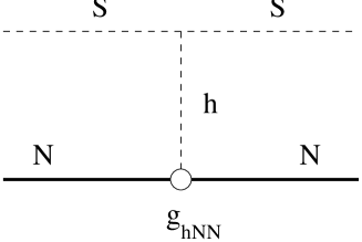
Figure 3: The Feynman graph relevant to scalar-nucleon elastic scattering.

The Feynman diagram describing elastic $S$-particle collisions with nucleons and nuclei is given by $t$-channel Higgs exchange, as shown in fig. (3). If we write, for slowly-moving spin-$J$ nuclei, the relevant nuclear matrix element as

$$\frac{1}{2J+1}\sum_{\rm spins}\Bigl{|}\langle N^{\prime}|\sum_{f}y_{f}\overline{f}f|N\rangle\Bigr{|}^{2}\approx\frac{|{\cal A}_{\scriptscriptstyle N}|^{2}}{(2\pi)^{6}},$$ (4.1)

then the nonrelativistic elastic scattering cross section obtained by evaluating fig. (3) becomes

$$\sigma_{\rm el}=\frac{\lambda^{2}v_{\scriptscriptstyle EW}^{2}|{\cal A}_{\scriptscriptstyle N}|^{2}}{\pi}\;\left(\frac{m_{*}^{2}}{m_{\scriptscriptstyle S}^{2}m_{h}^{4}}\right),$$ (4.2)

where $m_{*}=m_{\scriptscriptstyle S}m_{\scriptscriptstyle N}/(m_{\scriptscriptstyle S}+m_{\scriptscriptstyle N})$ is the reduced mass for the collision.

Modelling the nucleus as $A$ independent nonrelativistic nucleons leads to the expectation that ${\cal A}_{\rm nucleus}\approx A{\cal A}_{\rm nucleon}$, making it convenient to relate the elastic cross sections for nuclei and nucleons by

$$\sigma_{\rm el}(\hbox{nucleus})=\frac{A^{2}m_{*}^{2}(A,S)}{m_{*}^{2}(p,S)}\;\sigma_{\rm el}(\hbox{nucleon}),$$ (4.3)

The Higgs charge of the nucleon can be related to the nucleon mass and the trace anomaly, following ref. [31]. The result is sensitive to the mass of the strange quark and its content in the nucleon in the 0⁺ channel. Taking the strange quark mass to be 170 MeV and $\langle N|\bar{s}s|N\rangle\simeq 0.7$, (see, for example, Ref. [32]), we deduce the estimate:

$${\cal A}_{\rm nucleon}=g_{\scriptscriptstyle hNN}\approx\frac{340\leavevmode\nobreak\ {\rm MeV}}{v_{\scriptscriptstyle EW}},$$ (4.4)

leading to

$$\sigma_{\rm el}(\hbox{nucleon}) \approx \left(\frac{\lambda\leavevmode\nobreak\ 340\leavevmode\nobreak\ {\rm MeV}}{m_{h}^{2}}\right)^{2}\leavevmode\nobreak\ \left(\frac{m_{p}}{\pi(m_{p}+m_{\scriptscriptstyle S})}\right)^{2}$$ (4.5)

$$= \lambda^{2}\left(\frac{100\leavevmode\nobreak\ {\rm GeV}}{m_{h}}\right)^{4}\left(\frac{50\leavevmode\nobreak\ {\rm GeV}}{m_{\scriptscriptstyle S}}\right)^{2}\leavevmode\nobreak\ \Bigl{(}20\times 10^{-42}\leavevmode\nobreak\ {\rm cm}^{2}\Bigr{)}.$$

4.1 Recoil Experiments

It is instructive to see what kind of cross section is implied by the primordial cosmic abundance relation, $\lambda(m_{\scriptscriptstyle S})$. Using $m_{h}=120$ GeV and $m_{\scriptscriptstyle S}=40$ GeV, the abundance condition $0.1<\Omega_{s}h^{2}<0.3$ implies $0.05\mathrel{\raise 1.29167pt\hbox{$<$\kern-7.5pt\lower 4.30554pt\hbox{$\sim$}}}\lambda\mathrel{\raise 1.29167pt\hbox{$<$\kern-7.5pt\lower 4.30554pt\hbox{$\sim$}}}0.085$. Using these in eqs. (4.5) then gives $5\times 10^{-44}$ cm${}^{2}\mathrel{\raise 1.29167pt\hbox{$<$\kern-7.5pt\lower 4.30554pt\hbox{$\sim$}}}\sigma_{\rm el}(\hbox{nucleon})\simeq 1.5\times 10^{-43}$ cm², which is about a factor of 20 smaller than the range of nucleon scattering cross sections which are accessible in the DAMA and CDMS experiments [6, 22].

Figure 4: The predictions for the elastic cross section, $\sigma_{\rm el}$, as a function of $m_{\scriptscriptstyle S}$, which follows from the $\lambda(m_{\scriptscriptstyle S})$ dependence dictated by the cosmic abundance. Also shown by a dashed line is the exclusion limit from the CDMS experiment [6] .

Fig. (4) shows how the scattering cross section we obtain in this fashion is related to current experimental limits, under the standard assumption that the mass density of $S$-particles in our galactic halo is 0.3 GeV/cm³, having velocities of order 200 km/sec. This plot shows the lowest possible values of the cross sections, as it uses the maximum possible abundance $\Omega_{s}h^{2}=0.3$. For smaller values of the cosmic abundance, $\lambda^{2}$ is higher and the cross sections could be up to three times larger than those shown in fig. (4). The predictiveness of the $\lambda-m_{\scriptscriptstyle S}$ relation makes this model much easier to falsify than are more complicated models, with much of the parameter space covered by the next generation of experiments [4]. Most importantly, the projected sensitivities of the CDMS-Soudan and Genius experiments will completely cover the range $m_{\scriptscriptstyle S}\leq 50$ GeV, for values of the Higgs mass between 110 and 140 GeV. As we show in the next section, this range of masses and coupling constants has important implications for the Higgs searches at colliders. On the other hand, there exists the possibility of completely “hiding” the dark matter by choosing $0.4m_{h}\mathrel{\raise 1.29167pt\hbox{$<$\kern-7.5pt\lower 4.30554pt\hbox{$\sim$}}}m_{\scriptscriptstyle S}\leq 0.5m_{h}$. In this case annihilation at freeze-out is very efficient, requiring small $\lambda$’s which lead to elastic cross sections suppressed to the level of $10^{-48}$ cm². These levels of sensitivity to $\sigma_{\rm el}(\hbox{nucleon})$ are not likely to be achieved in the foreseeable future.

Our model of a singlet real scalar predicts a smaller signal for underground detectors than does a model where the dark matter consists of $N$ singlet scalars (including the model considered in ref. [10], for which $N=2$). This is because the abundance of every individual species must be $1/N$ of the total dark matter abundance, $\Omega_{i}=\Omega_{\rm tot}/N$. This requires a larger annihilation rate at freeze-out for every species, and so an enhancement of the coupling $\lambda$ by $\sqrt{N}$, relative to the values of coupling constant calculated in this paper. By contrast, since the local halo density does not depend on $N$, the signal from an $N$-component scalar dark matter model will be $N$ times larger than what is found here for the signal from our single-component dark matter model.

4.2 High-Energy Neutrino Searches

The elastic cross section calculated above, $\sigma_{\rm el}$, also controls the expected flux of high-energy neutrinos which would be emitted by $S$ particles which are captured at the centre of the sun or the earth. It does so because of the following scenario, which describes how the abundance of such particles is determined.

$S$ particles which lose enough energy through scattering get trapped in the gravitational field of the sun or the earth. Further scattering permits them to further dissipate their energy, until they eventually accumulate at the solar (or terrestrial) center. Their density at the centre grows until the accumulation rate precisely balances their rate of removal due to pair annihilation, leading to an equilibrium abundance. Because of this balance the total rate of annihilations may be computed given the capture rate, and so also given the elastic scattering rate.

The detection of these captured particles is based on observing the high-energy neutrinos which are among the production products of these annihilations. These neutrinos can escape from the solar (or terrestrial) centre, and can be detected by neutrino telescopes, which look for the energetic muons which are produced when the neutrinos interact with rock or ice in the detectors’ immediate vicinity. In this way a signal is predicted for detectors like Baksan, Kamiokande, Macro, Amanda and others.

To predict this signal we use the results of Ref. [33], which follows the original treatment in Refs. [34], and estimate the neutrino flux at the surface of the earth due to $S$-particle annihilation in the sun as

$$\phi_{\nu\odot}\simeq(560\hbox{cm}^{-2}\hbox{s}^{-1})\;N_{\rm eff}\;\sigma_{\rm el,36}\;\frac{\mbox{GeV}^{2}}{m_{\scriptscriptstyle S}^{2}}.$$ (4.6)

In this formula $N_{\rm eff}$ is the average number of neutrinos produced per annihilation event, and $\sigma_{\rm el,36}$ is the $S$-proton elastic scattering cross section in units of $10^{-36}$ cm².

The determination of $N_{\rm eff}$ requires a study of the final states which are available in $S$ annihilations, which are mediated by $s$-channel Higgs-exchange, as in Fig. (1). The number of neutrinos produced depends on the value of $m_{\scriptscriptstyle S}$, which controls whether the main annihilation products are $W^{+}W^{-}$, $b\bar{b}$ or other light hadrons. (Direct branching to a pair of neutrinos is obviously very small for Higgs-mediated decays.) The total production of energetic neutrinos turns out to be quite significant, as all decay products typically produce final state neutrinos (and so non-vanishing $N_{\rm eff}$) due to cascades of weak decays. The resulting value for $N_{\rm eff}$ and the energy spectra of the produced neutrinos have been meticulously simulated by Ritz and Seckel in Ref. [35] and more recently by Edsjo [36].

To obtain an upward-going flux of energetic muons, one must compute the probability that a neutrino directed towards the detector produces a muon at the detector. This probability, $P(E)$, is a quadratically rising function of neutrino energy, $E$, which must be convoluted with the computed neutrino fluxes [37, 38]. Approximating this probability as $P(E)\sim 10^{-8}(E/{\rm 100\leavevmode\nobreak\ GeV})^{2}$, we use the results of Ref. [35] for $60$ GeV $b$ quarks injected into the center of the sun, which predicts $N_{\rm eff}$ to be $0.3$. The second moment of the neutrino energy distribution, $N_{\rm eff}\,\langle(E/m_{\scriptscriptstyle S})^{2}\rangle$ becomes 0.006. Extrapolating these results to the case $m_{\scriptscriptstyle S}=50$ GeV gives

$$\phi_{\mu}=0.8\times 10^{-14}\left(\frac{\sigma_{\rm el}(\hbox{nucleon})}{10^{-44}\leavevmode\nobreak\ {\rm cm}^{2}}\right){\rm cm}^{-2}{\rm s}^{-1}.$$ (4.7)

This should be compared with experimental limits on the flux of energetic upward muons (as obtained, for example, by the Kamiokande, MACRO and Baksan experiments, [26, 27, 28]), which is $\phi_{\mu}\mathrel{\raise 1.29167pt\hbox{$<$\kern-7.5pt\lower 4.30554pt\hbox{$\sim$}}}1.4\times 10^{-14}$ cm^-2s^-1. Using the value of $\sigma_{\rm el}(\hbox{nucleon})$ suggested by abundance calculations (c.f. eq. (4.5)), we can see that the predicted flux is right at the level of current experimental sensitivity. The constraints on the flux coming from the center of the earth can be equally important [10].

There are, of course, caveats to the blanket use of these constraints, since loopholes can exist for some values of the parameters. For instance, according to Ref. [35], the average energy of the neutrinos is about 10% of $m_{\scriptscriptstyle S}$, and so for lower values of $m_{\scriptscriptstyle S}$ the muons passing through the detectors might be close to or below the experimental thresholds. We conclude that although the prospects are good for observable signals in these detectors, more detector–oriented studies need to be done in order to exploit fully the limits which may result.

5 Implications for Collider Experiments

We next turn to the implications of the model for Higgs searches at colliders. As we saw from the primordial abundance constraints, over most of parameter space $\lambda\simeq O(0.1)-O(1)$. This means that real or virtual Higgs production might frequently also be associated with $S$ production, potentially leading to strong missing energy signals. (See refs. [15] for discussions of the implications of related scalar models for collider experiments and refs. [40] for the discussion of invisible Higgs decay in supersymmetric models.) Since the extent to which this actually happens depends strongly on the $S$-particle mass, we consider the main alternatives successively.

5.1 $2m_{s}<m_{h}$

This is the most interesting possibility, since it permits the decay of the Higgs into a pair of $S$-particles. The decay width, calculated at tree level, is given by

$$\Gamma_{h\rightarrow SS}=\frac{\lambda^{2}v_{\scriptscriptstyle EW}^{2}}{8\pi m_{h}}\sqrt{1-\frac{4m_{\scriptscriptstyle S}^{2}}{m_{h}^{2}}}\qquad{\rm for}\qquad 2m_{\scriptscriptstyle S}<m_{h}.$$ (5.1)

Needless to say, since any produced $S$ particles are unlikely to interact within the detectors, the large values for $\lambda$ suggested by cosmic abundance can give a very large invisible decay width to the Higgs, without changing the Higgs’ other Standard Model couplings. This fact obviously has many consequences for Higgs searches at colliders, since Higgses will be produced at the rates expected in the Standard Model, but will mostly decay invisibly into $S$ pairs. To quantify this observation we calculate the ratio of the above invisible width to the width for the decay $h\to\tau^{+}\tau^{-}$:

$$\frac{\Gamma_{\scriptscriptstyle h\rightarrow SS}}{\Gamma_{\scriptscriptstyle h\rightarrow\tau^{+}\tau^{-}}}=\frac{\lambda^{2}v_{\scriptscriptstyle EW}^{4}}{m_{h}^{2}m_{\tau}^{2}}\sqrt{1-\frac{4m_{\scriptscriptstyle S}^{2}}{m_{h}^{2}}}.$$ (5.2)

Using the usual cosmic abundance constraints, obtained in Section 3, one can see that this ratio can be as large as 1000, so that the decay of the Higgs into a pair of $S$ scalars is by far the more probable event. More useful information is given, however, by another ratio,

$$R=\frac{{\rm Br}_{h\rightarrow\tau^{+}\tau^{-}}(SM+S)}{{\rm Br}_{h\rightarrow\tau^{+}\tau^{-}}(SM)}=\frac{\Gamma_{h,\leavevmode\nobreak\ total}(SM)}{\Gamma_{h\rightarrow SS}+\Gamma_{h,\leavevmode\nobreak\ total}(SM)},$$ (5.3)

where the last equality uses the fact that Higgs production rates are not affected by the existence of a new scalar. $R$ quantifies the deterioration (relative to the SM result) of the expected signal for Higgs decaying into visible modes due to the adding of the new scalar. We plot $R$, in fig. (5), against $m_{\scriptscriptstyle S}$ up to the Higgs mass for the same values of $m_{h}$ and $\lambda$ as in fig. (2).

Figure 5: The ratio, $R$, of the total Higgs width in the Standard model over the same width in the Standard Model supplemented by the singlet scalar, plotted as a function of $m_{\scriptscriptstyle S}$.

As is clear from the plot, for $m_{h}=100$, 120 and 140 GeV and $2m_{\scriptscriptstyle S}<m_{h}$ the invisible width dominates the total width everywhere except in the immediate vicinity of $2m_{\scriptscriptstyle S}=m_{h}$. $R$ shrinks near this point for two reasons. First, $m_{h}$ near $2m_{\scriptscriptstyle S}$ is close to threshold for producing two $S$ particles in $h$ decay, and so the invisible rate is phase-space suppressed in this region. More importantly, the size of the coupling, $\lambda$, allowed by abundance arguments is smaller for $m_{\scriptscriptstyle S}$ in this region, due to the enhancement of the primordial annihilation cross section due to proximity with the Higgs pole.

However, the plot also shows that the presence of the invisible width already downgrades the expected signal by a factor of 10 or more when $m_{S}\simeq 0.3m_{h}$ GeV for $m_{h}=120$ or 140 GeV. This means that over 10 times more Higgs particles must be produced in order to reach the same level of signal in all visible decay modes, as compared to what is expected purely within the Standard Model. This implies a tremendous suppression of the observable Higgs signal at the LHC and especially at the Tevatron — possibly even precluding its discovery at these machines (see, however, ref. [41, 42, 43] for a more optimistic point of view). The main Higgs production reaction in this case would be two jets plus missing energy, a process having enormous backgrounds in hadron machines.

On the other hand, for $m_{h}$ close to or above the $W^{+}W^{-}$ threshold, the similarity in size between $\lambda$ and the electromagnetic coupling, $e$, implies that the invisible width does not completely dominate other decay modes. In such a case (fig. (5), $m_{h}=$200 GeV) the decline in $R$ is not dramatic, and the existence of an invisible signal need not preclude finding the Higgs in a hadron machine.

More can be said about an invisibly decaying Higgs at $e^{+}e^{-}$ machines. Although the missing energy signal would be missed in an orthodox Standard-Model Higgs search, such as one based on $b$-tagging, more model-independent searches have been performed for scalars produced with Standard Model cross sections, but decaying invisibly. These searches at LEP exclude such an invisibly-decaying Higgs unless $m_{h}\mathrel{\raise 1.29167pt\hbox{$>$\kern-7.5pt\lower 4.30554pt\hbox{$\sim$}}}106.7$ GeV [44].

5.2 $2m_{\scriptscriptstyle S}>m_{h}$

For this mass pattern, $S$ particles cannot be produced by real Higgs decays, and so arise only through virtual Higgs exchange. Again, once produced, these particles are not expected to interact within the detector and so look like missing energy above an energy threshold, $E\geq 2m_{\scriptscriptstyle S}$.

A missing-energy signal can be searched for at $e^{+}e^{-}$ colliders, where the backgrounds are very well understood. Since hadronic machines are unlikely places for seeing such a signal, we do not consider them further here.

Figure 6: The dominant mechanism for pair-producing $S$-particles at LEP, via $s$-channel Higgs exchange.

Fig. (6) shows the main mechanism for the production of two $S$ scalars at LEP (or at a linear collider). The differential cross-section for this process which results from the evaluation of this graph is as follows:

$${\frac{d\sigma_{\scriptscriptstyle e^{+}e^{-}\rightarrow ZSS}}{dt\leavevmode\nobreak\ du}}=\frac{(g_{\scriptscriptstyle L}^{2}+g_{\scriptscriptstyle R}^{2})\lambda^{2}v_{\scriptscriptstyle EW}^{2}|a_{z}|^{2}}{16(2\pi)^{3}s}\leavevmode\nobreak\ \left(\frac{e}{s_{w}c_{w}}\right)^{2}\left[{\frac{s+(t-m_{\scriptscriptstyle Z}^{2})(u-m_{\scriptscriptstyle Z}^{2})/m_{\scriptscriptstyle Z}^{2}}{(s-m_{\scriptscriptstyle Z}^{2})^{2}+\Gamma_{\scriptscriptstyle Z}^{2}m_{\scriptscriptstyle Z}^{2}}}\right]$$

$$\times\left[{\frac{1}{s+t+u-m_{\scriptscriptstyle Z}^{2}-m_{h}^{2}}}\right]^{2}\sqrt{1-\frac{4m_{\scriptscriptstyle S}^{2}}{(s+t+u-m_{\scriptscriptstyle Z}^{2})}}.$$ (5.4)

Here we follow the notation of ref. [39], with $g_{\scriptscriptstyle L}=-\,\frac{1}{2}+s_{w}^{2}$ and $g_{\scriptscriptstyle R}=s_{w}^{2}$ parameterizing charged-lepton couplings to the $Z$ boson, $a_{z}=em_{\scriptscriptstyle Z}/(c_{w}s_{w})$ being the effective coupling of the Higgs to $Z$ boson, and $s_{w}$ and $c_{w}$ denoting the sine and cosine of the Weinberg angle. The Mandelstam variables, $s$, $t$ and $u$, are defined as for a 2-body to 2-body process, with their sum given by $s+t+u=m_{\scriptscriptstyle Z}^{2}+Q^{2}$, where $m_{\scriptscriptstyle Z}$ is the $Z$-boson mass and $Q^{2}$ is the square of the invariant mass of the two $S$-particles.

Expression (5.4) also applies to the previous case, where $2m_{\scriptscriptstyle S}<m_{h}$, in which case the cross section is dominated by the Higgs pole, corresponding to real Higgs production. It is clear that the constraint on the missing energy implied by eq. (5.4), and the experimentally measured values for such a process at LEP, cannot lead to a limit on the invariant mass of two $S$ particles better than 100 GeV for a Higgs mass of around 100 GeV. For larger values of $m_{h}$ a possible bound on the invariant mass of the $S$ pair is considerably relaxed.

6 Conclusions

We have presented the first study of the minimal model for non-baryonic dark matter, which consists of the Standard model plus a singlet scalar. This model is characterized by one additional real scalar field and three new parameters. The absence of linear and cubic terms in $S$ is required to ensure that the the new scalar is sufficiently stable to contribute significantly to the dark matter currently present in the Universe. This stability also precludes the development of a nonzero v.e.v. for $S$. The study of the model’s scalar potential shows that electroweak symmetry is spontaneously broken while $\langle S\rangle$ vanishes for a significant domain of parameter space.

At the renormalizable level the three parameters describe the $S$ particle mass, its self-coupling and its couplings to other Standard Model fields, which all are mediated by a coupling to the Standard Model Higgs, of the form $\lambda S^{2}(H^{\dagger}H)$. The simplicity of this coupling significantly simplifies the calculations of primordial abundances and observable signals at colliders and underground detectors, making the resulting predictions more certain. The primordial abundance is governed mainly by the annihilation of $S$-particles via $s$-channel Higgs exchange. If the mass of the Higgs is not too close to $2m_{\scriptscriptstyle S}$, the observed abundance of dark matter is achieved by a most natural choice for the coupling, $\lambda\sim O(0.1-1)$.

These large values of $\lambda$ lead to nuclear elastic cross sections which are $\sim 10^{-43}$ cm² in size. This is slightly below the limits of sensitivity of the DAMA and CDMS experiments, but is likely to be detectable at future experimental facilities. Thus, the direct detection of $S$ particles is not yet ruled out, and is easily feasible within the near future! Our minimal model is unable to reconcile the DAMA and CDMS results, and so predicts that one or the other is incorrect.

Cross sections this large also lead to a significant flux of high-energy neutrinos generated by $S$ annihilation at the centers of the earth and the sun, at levels potentially accessible to large neutrino detectors. We give here only an estimate of the expected flux, and we believe the encouraging results motivate further work to simulate the expected neutrino and muon spectra and intensities. It would also be intriguing to repeat the numerical analysis of ref. [10], updated with the Higgs masses favored by modern collider results.

Large values for $\lambda$ may also lead to the significant missing-energy signals at colliders, corresponding to the production of a pair of $S$-particles. This signal is unlikely to be seen at hadronic machines, where the background events (two jets plus missing energy) will have much larger cross-sections. Lepton colliders, such as LEP or NLC are needed. The possible existence of $S$-particles with a mass smaller than half of the Higgs boson mass poses a significant threat to Higgs searches at the Tevatron and LHC. Indeed, in this case the invisible decay of the Higgs boson can be many orders of magnitude larger than the search modes, making the Higgs effectively invisible. For intermediate Higgs masses, up to 140 GeV and higher, the pair production of $W$ bosons introduces a nonnegligible visible width and so saves the Higgs searches. It is important that in the dangerous domain of parameter space, $2m_{\scriptscriptstyle S}<m_{h}<140$ GeV, the size of the elastic cross-section, $\sigma_{\rm el}$, is limited from below to be larger than $10^{-44}$ cm². If this were indeed the case, the next generation of the underground detectors would likely discover the recoil signal.

Because the self-coupling, $\lambda_{\scriptscriptstyle S}$, is unconstrained by the abundance condition, one might hope to use models of this sort to produce a strongly-interacting dark matter candidate, a possibility recently advocated in ref. [12, 14]. Unfortunately, this proposal would also require a rather small mass for the $S$-scalars (1 GeV or less), and since $\lambda$ cannot be small for such masses, one is led to a fine-tuned (ppm) cancellation between $\lambda v_{EW}^{2}$ and the “bare” mass $m_{0}^{2}$. Worse, having $m_{\scriptscriptstyle S}$ be 500 MeV or smaller pushes $\lambda$ to the very limits of our perturbative analysis.

It remains an interesting challenge to construct a non-minimal model of strongly-interacting dark matter along the present lines. One possibility is to suppress $\lambda$ to evade the fine-tuning problem, and set the freeze-out abundance by a set of non-renormalizable operators of dimension 6 and higher. Another possibility for having light and strongly interacting scalar dark matter requires $\lambda$ to be very small, scalar particles to be out of equilibrium at all temperatures, and their abundance to be fine-tuned (for example, using inflationary scenarios). The suppression of the coupling to the Higgs, strong self-interaction and a low mass for $S$ could be simultaneously achieved in models where $S$ is composite [21], in which case there is unlikely to be significant impact on Higgs physics.

Our pursual here of a more model-independent approach to the physics of dark matter particles is ultimately stimulated by the maturity of current dark-matter detection efforts. As the data erodes the large parameter space of the popular neutralino models, or if a dark matter candidate is eventually found, a reliable interpretation of the experiments can only be found by comparing with a wide variety of explanatory models. Our proposal in this paper marks the absolute minimum of complexity required by such a model, and from this minimality springs its predictiveness. It is also generic in the sense that it is the most general renormalizable model consistent with the assumed particle content and symmetries. As such, it captures the implications of any models whose implications for dark matter arise from a low energy spectrum which contains only these particles and symmetries. We believe that further model–building efforts are in order as experimental developments progress.

Acknowledgements

We thank G. Couture, T. Falk, L. Kofman, G.Mahlon, K. Olive, S. Rudaz and M. Voloshin for usefull discussions and comments. M.P. wishes to thank the Physics Departments of McGill University and the University of Québec at Montréal, where a significant portion of this work was carried out. M.P. and T. t V.’s research was funded by the US Department of Energy under grant number DE-FG-02-94-ER-40823, and C.B. acknowledges the support of NSERC (Canada), FCAR (Québec) and the Ambrose Monell Foundation.

References

- [1] M. S. Turner, Phys. Rept. 333-334 (2000) 619.
- [2] See e.g. G. Jungman, M. Kamionkowski and K. Griest, Phys. Rept. 267 (1996) 195, L. Bergstrom, Rept. Prog. Phys. 63 (2000) 793.
-
[3]
H. Pagels and J. R. Primack, Phys. Rev. Lett. 48 (1982) 223;
J. Ellis, J.S. Hagelin, D.V. Nanopoulos, K.A. Olive and M. Srednicki, Nucl. Phys. B238 (1984) 453.
For a recent study, see: J. Ellis, T. Falk, G. Ganis and K. A. Olive, Phys. Rev. D62 (2000) 075010. - [4] D. Caldwell, Nucl. Phys. B70 (Proc. Suppl.) (1999) 43.
-
[5]
R. Bernabei et al., preprint ROM2F/2000/01 and
INFN/AE-00/01;
R. Bernabei et al., Phys. Lett. B450 (1999) 448. - [6] R. Abusaidi et al., Phys. Rev. Lett. 84 (2000) 5699.
- [7] M. Pospelov and T. ter Veldhuis, Phys. Lett. B480 (2000) 181.
- [8] M. Veltman and F. Yndurain, Nucl. Phys. B325 (1989) 1.
- [9] V. Silveira and A. Zee, Phys. Lett. B161 (1985) 136.
- [10] J. McDonald, Phys. Rev. D50 (1994) 3637.
-
[11]
R. Flores and J. M. Primack, Ap. J. 427
(1994) L1;
B. Moore, Nature 370 (1994) 620;
B. Moore et al., M.N.R.A.S. 310 (1999) 1147, Ap. J. 524 (1999) L19;
A. A. Klypin et al., Ap. J. 522 (1999) 82, Ap. J. 554 (2001) 903. - [12] N. Spergel and P.J. Steinhardt, Phys. Rev. Lett. 84 (2000) 3760.
- [13] N. Yoshida et al., Ap. J. 544 (2000) L87.
- [14] M.C. Bento et.al., Phys. Rev. D62 (2000) 041302.
-
[15]
R. S. Chivukula and M. Golden,
Phys. Lett. B267, (1991) 233;
R. S. Chivukula, M. Golden and M. V. Ramana, Phys. Lett. B293, (1992) 400;
T. Binoth and J.J. van der Bij, hep-ph/9511467;
T. Binoth and J. J. van der Bij, Z. Phys. C75 (1997) 17
R. Akhoury, J. J. van der Bij and H. Wang, hep-ph/0010187. -
[16]
S. Coleman, Nucl. Phys. B262, (1985) 263.
For a recent discussion, see: D. A. Demir, Phys. Lett. B450, 215 (1999). - [17] L. Kofman, A. Linde and A.A. Starobinsky, Phys. Rev. D56 (97) 3258.
- [18] E.W. Kolb and M.S. Turner, The Early Universe, Addison-Wesley, 1990.
- [19] K. Griest and D. Seckel, Phys. Rev. D43 (1991) 3191.
- [20] M. Voloshin, Sov. J. Nucl. Phys. 44 (1986) 478.
- [21] A. Faraggi and M. Pospelov, hep-ph/0008223.
- [22] R. Bernabei et al., Phys. Lett. B389 (1996) 757.
- [23] P.F. Smith et al., Phys. Lett. B376 (1996) 299.
- [24] M. Beck et al., Phys. Lett. B336 (1994) 141.
- [25] A. Morales et al., Phys. Lett. B489 (2000) 268.
- [26] M. Mori et al., Phys. Rev. D48 (1993) 5505.
- [27] M. Ambrosio et al., Phys. Rev. D60 (1999) 082002.
- [28] M.M. Boliev, et al., Nucl. Phys. B48 (Proc. Suppl.) (1996) 83.
- [29] E. Andres et al., Nucl. Phys. Proc. Suppl. 91 (2000) 4232.
- [30] A. Okada, Nucl. Phys. Proc. Suppl. 91 (2000) 423.
- [31] M.A. Shifman, A.I. Vainshtein, and V.I. Zakharov, Phys. Lett. B78 (1978) 264.
- [32] A Zhitnitsky, Phys. Rev. D55 (1997) 3006.
- [33] A. E. Faraggi, K. A. Olive and M. Pospelov, Astropart. Phys. 13 (2000) 31.
-
[34]
J. Silk, K.A. Olive, and M. Srednicki, Phys. Rev. Lett. 55 (1985) 257;
M. Srednicki, K.A. Olive, and J. Silk, Nucl. Phys. B279 (1987) 804. - [35] S. Ritz and D. Seckel, Nucl. Phys. B304 (1988) 877.
- [36] J. Edsjo, Nucl. Phys. Proc. Suppl. 43 (1995) 265.
- [37] T.K. Gaisser and T. Stanev, Phys. Rev. D31 (1985) 2770.
- [38] M. Honda and M. Mori, Prog. Theor. Phys. 78 (1987) 963.
- [39] C. Burgess, J. Matias and M. Pospelov, hep-ph/9912459.
-
[40]
H. Haber, D. Dicus, M. Drees, and X. Tata, Phys. Rev. D37 (1987) 1367;
K. Griest and H. E. Haber, Phys. Rev. D37 (1988) 719;
A. Djouadi, J. Kalinowski, and P.M. Zerwas, Z. Phys. C57 (1993) 569;
J. L. Lopez, D. V. Nanopoulos, H. Pois, X. Wang, and A. Zichichi, Phys. Rev. D48 (1993) 4062. - [41] J. F. Gunion, Phys. Rev. Lett. 72 (1994) 199.
- [42] S. P. Martin and J. D. Wells, Phys. Rev. D60 (1999) 035006.
- [43] O. J. Eboli and D. Zeppenfeld, Phys. Lett. B495 (2000) 147.
-
[44]
P. I. Kemenes, talk given at the XXXth
International Conference on High Energy Physics, Osaka 2000;
Searches for Higgs Bosons: Preliminary Combined Results using LEP Data
Collected at Energies up to 202 GeV, the ALEPH, DELPHI, L3 and OPAL Collaborations
(P. Bock et al.), preprint CERN-EP-2000-055, Apr 2000;
This limit has recently changed appreciably, since the bound from previous running gave a limit of 94.5 GeV (ALEPH). See:
ALEPH Collaboration (R. Barate et al.), Phys. Lett. B465 (1999) 349;
DELPHI Collaboration (P. Abreu et al.), Phys. Lett. B459 (1999) 367;
L3 Collaboration (M. Acciarri et al.), Phys. Lett. B485 (2000) 85;
OPAL Collaboration (G. Abbiendi et al.), Eur.Phys.J. C12 (2000) 567.