Exclusive hadronic $\tau$ decays in the resonance effective action of QCD

Abstract

Until present the study of the form factors associated to the vector and axial–vector components of the hadronic weak current has been carried out with a plethora of modelizations of the underlying strong interactions. While of importance to get an understanding of the dynamics involved, the amount and quality of the experimental data start to show some discrepancies with the analysed models. Moreover, and from a theoretical point of view, most of these models are not consistent with quantum chromodynamics (QCD). We propose a QCD–based model–independent procedure to analyse those decays through the use of the resonance chiral theory, the low–energy effective action of QCD in the relevant resonance region. Within this framework we study the hadronic off–shell width of the $\rho$ meson and the vector form factor of pion in $\tau^{-}\rightarrow\pi^{-}\pi^{0}\nu_{\tau}$. We also comment on the $\tau^{-}\rightarrow(\pi\pi\pi)^{-}\nu_{\tau}$ decay.

1 Introduction

The study of matrix elements of hadronic currents in the low–energy regime is a long–standing problem of particle physics driven by our poor knowledge of non–perturbative QCD. In this framework exclusive hadronic $\tau$ decays ($\tau^{-}\rightarrow H^{-}\nu_{\tau}$) provide an excellent dynamical system to explore, due to the hadronically clean initial state and the factorization between lepton and hadron sectors generically given, in the Standard Model, by

$$M\; = \frac{\displaystyle G_{F}}{\displaystyle\sqrt{2}}\,V_{CKM}\,\overline{u}_{\nu}\gamma^{\mu}(1-\gamma_{5})u_{\tau}\,H_{\mu}\,,$$

$$H_{\mu} = \langle\,H\,|\,(V_{\mu}-A_{\mu})e^{iL_{strong}}\,|\,0\,\rangle\,.$$ (1)

Symmetries help us to define a decomposition of $H_{\mu}$ in terms of the allowed Lorentz structure of implied momenta and a set of functions of Lorentz invariants, the form factors $F_{i}^{H}$,

$$H_{\mu}\;=\;\sum_{i}\underbrace{\;\,(\,\ldots\,)_{\mu}^{i}\;\,}_{Lorentz\,struc.}F_{i}^{H}(q^{2},\ldots)\;.$$ (2)

Form factors are the goal of the hadronic matrix elements evaluation and, as can be noticed from the definition of $H_{\mu}$ in Eq. (1), are a strong interaction related problem in a non–perturbative regime.

In the last years experiments like ALEPH, CLEO-II, DELPHI and OPAL [1, 2, 3] have collected an important amount of experimental data on exclusive channels. Analyses of these data are carried out using the TAUOLA library [4] that includes modelizations of the hadronic matrix elements. Though heuristically based in expected consequences of QCD, models include simplifying assumptions that may be are not well controlled from QCD itself. Therefore, while of importance to get an understanding of the dynamics involved, models can be misleading and provide a delusive interpretation of data. Of particular importance are the processes with two and three pseudoscalars in the final state. TAUOLA describes these using the Kühn and Santamaria model [5]. In order to find out the size of the hadronic uncertainties hidden in the modelization a common procedure is to use another model, typically the Gounaris and Sakurai [6], and then the error is estimated from the difference between the results of both modelizations [2].

The question that we address in this note is how much we can say about the semileptonic form factors in a model–independent way. We will study here the pion vector form factor in $\tau^{-}\rightarrow\pi^{-}\pi^{0}\nu_{\tau}$ and the problem of defining a hadronic off–shell width of meson resonances. We comment shortly on the $\tau^{-}\rightarrow(\pi\pi\pi)^{-}\nu_{\tau}$ decay.

2 Model–independent knowledge

Our study is intended to extract information by exploiting well–known basic properties of S–matrix theory and QCD. These provide precise constraints to take into account both on the hadronic off–shell widths of meson resonances and the relevant form factors. We sketch here the pertinent features.

2.1 S–matrix theory properties

On general grounds local causality of the interaction translates into the analyticity properties of amplitudes and, correspondingly, of form factors. Being analytic functions in complex variables the behaviour of form factors at different energy scales is related and, moreover, they are completely determined by their singularities. Dispersion relations embody rigorously these properties and are the appropriate tool to enforce them.

In addition unitarity must be satisfied in all physical regions. This S–matrix property provides precise information on the relevant contributions to the spectral functions of correlators of hadronic currents. These are closely related to the form factors.

Unitarity and analyticity complement each other. We will see later on, in some examples, how these S–matrix theory features help in the construction of hadronic observables.

2.2 QCD

Though we do not know how to evaluate low–energy hadronic matrix elements from QCD itself, a theorem put forward by S. Weinberg [7] and worked out by H. Leutwyler [8] sets that, if one writes down the most general possible Lagrangian, including all terms consistent with assumed symmetry principles, and then calculates matrix elements with this Lagrangian to any given order of perturbation theory, the result will be the most general possible S–matrix consistent with analyticity, perturbative unitarity, cluster decomposition and the principles of symmetry that have been specified. It is in this statement that part of the model–independent work on low–energy hadronic physics has been based upon.

Massless QCD is symmetric under global independent $SU(N_{F})$ rotations of left– and right–handed quark fields

$$q_{L}\,\rightarrow\,h_{L}\,q_{L}\,\, \;\;h_{L}\in SU(N_{F})_{L},$$ ,

$$q_{R}\,\rightarrow\,h_{R}\,q_{R}\,\, \;\;h_{R}\in SU(N_{F})_{R},$$ , (3)

where $N_{F}=2,3$ is the number of light flavours. This is the well–known $SU(N_{F})_{L}\otimes SU(N_{F})_{R}$ chiral symmetry of QCD [7, 9, 10, 11]. Quark masses break explicitly this symmetry but what is more relevant is that it seems it is also spontaneously broken. Though a rigorous prove of this feature has only been achieved in the large number of colours limit [12], the known phenomenology supports that statement. Goldstone theorem demands the appearance of a phase of massless bosons associated to the broken generators of the symmetry and their quantum numbers happen to correspond to those of the lightest octet ($N_{F}=3$) of pseudoscalars : $\pi$, $K$ and $\eta$. Their non–vanishing masses are due to the explicit breaking of chiral symmetry through quark masses.

This Goldstone phase is fortunate because it provides an energy gap into the meson spectrum between the octet of pseudoscalars and the heavier mesons starting with the $\rho(770)$. We can take precisely the mass of this resonance $M_{\rho}$ as a reference scale to introduce effective actions of the underlying QCD:

a) $E\ll M_{\rho}$
      In this energy region chiral symmetry is the guiding principle to follow. The relevant effective theory of QCD is chiral perturbation theory ($\chi$PT) [7, 11] that exploits properly the chiral symmetry $SU(N_{F})_{L}\otimes SU(N_{F})_{R}$. In this effective action the active degrees of freedom are those of the octet of pseudoscalars and the heavier spectrum has been integrated out. As its own name implies, $\chi$PT is a perturbation theory in the momenta of pseudoscalars over a typical scale $\Lambda_{\chi}\sim 1\,\mbox{GeV}$. This entails that the interaction vanishes with the momentum, giving an example of dual behaviour between the effective action (perturbative at low energies) and QCD (where asymptotic freedom prevents a perturbative expansion in that energy regime). By demanding that the interaction satisfies chiral symmetry the complete structure of the operators, at a definite perturbative order, is defined. However chiral symmetry does not give any information on their couplings that, in general, carry the information of the contributions of heavier states that have been integrated out. Their study is outside the scope of $\chi$PT but some thorough developments have been achieved [13, 14].

$\chi$PT is a long–standing successful framework for the study of strong and weak processes at very low energies [15].

b) $E\simeq M_{\rho}$
      At $E\simeq 1\,\mbox{GeV}$ other meson states (mainly unstables) are active degrees of freedom to take into account. Chiral symmetry still provides the guide in the construction of the effective action of QCD, following the pioneering work of S. Weinberg [10] in which the new states are represented by fields that transform non–linearly under the axial part of the chiral group. For the lightest octet of resonances (vectors, axial–vectors, scalars and pseudoscalars) this procedure was carried out in Ref. [13] and the resulting effective action is called resonance chiral theory. As in $\chi$PT, chiral symmetry constraints the structure of the operators but gives no information on their couplings, that remain unknown, though they could be studied by using models. Resonance chiral theory provides, therefore, a model–independent parameterization of the processes involving resonances and pseudoscalars in terms of those couplings.

c) $E\gg M_{\rho}$
      At much higher energies the asymptotic freedom of QCD implies that a perturbative treatment of the theory is indeed appropriate. The study of this energy region is also important for low–energy hadron physics because we are able to evaluate, within QCD, the asymptotic behaviour of spectral functions and then to impose these constraints on the low–energy regime. This procedure is well supported at the phenomenological level.

To take advantage of the underlying QCD dynamics in the model–independent study of hadronic observables, we have to consider the entire view and how different energy regimes intertwine between themselves.

3 Hadronic off–shell width of meson resonances

Before addressing the issue of form factors in exclusive hadronic $\tau$ decays let us consider one of its basic elements : the off–shell width of meson resonances. We will focus in the width of the $\rho$ though the discussion is analogous for any meson resonance. In Ref. [16] it was pointed out that one could consider the evaluation of the off–shell $\rho$ width from the resonance chiral theory. The detailed account, that I shortly report here, has been developed in Ref. [17].

The resonance chiral effective theory with three flavours and including only vector meson resonances is given, at the lowest chiral order, by [13]

$${\cal L}_{\chi V}\,=\,{\cal L}_{\chi}^{(2)}\,+\,{\cal L}_{KV}\,+\,{\cal L}_{V}^{(2)}\;.$$ (4)

Here ${\cal L}_{\chi}^{(2)}$ is the ${\cal O}(p^{2})$ chiral Lagrangian

$${\cal L}_{\chi}^{(2)}\,=\,\frac{\displaystyle F^{2}}{\displaystyle 4}\,\langle\,u_{\mu}u^{\mu}\,+\,\chi_{+}\,\rangle\;,$$ (5)

where $F$ is the pion decay constant ($F\approx 92.4\,\mbox{MeV}$),

$$u_{\mu}\, = \,i\,[u^{\dagger}(\partial_{\mu}-ir_{\mu})u\,-\,u(\partial_{\mu}-i\ell_{\mu})u^{\dagger}\,]\;,$$

$$\chi_{+}\, = \,u^{\dagger}\chi u^{\dagger}\,+\,u\chi^{\dagger}u\;,$$

$$u\, = \,\exp\left(\frac{\displaystyle i}{\displaystyle\sqrt{2}F}\Pi\right)\,,$$ (6)

and $\Pi$ is the usual representation of the Goldstone fields

$$\Pi=\left(\begin{array}[]{ccc}\frac{\displaystyle\pi^{0}}{\displaystyle\sqrt{2}}\,+\,\frac{\displaystyle\eta_{8}}{\displaystyle\sqrt{6}}&\pi^{+}&K^{+}\\ \pi^{-}&-\frac{\displaystyle\pi^{0}}{\displaystyle\sqrt{2}}\,+\,\frac{\displaystyle\eta_{8}}{\displaystyle\sqrt{6}}&K^{0}\\ K^{-}&\overline{K^{0}}&-\frac{\displaystyle 2}{\displaystyle\sqrt{6}}\eta_{8}\end{array}\right).$$ (7)

In Eq. (5), $\langle A\rangle$ stands for a trace in flavour space. ${\cal L}_{\chi}^{(2)}$ has a $SU(3)_{L}\otimes SU(3)_{R}$ chiral gauge symmetry supported by the external fields $\ell_{\mu}$, $r_{\mu}$ and $\chi$.

In Eq. (4), ${\cal L}_{KV}$ is the kinetic Lagrangian of vector mesons and ${\cal L}_{V}^{(2)}$ describes the chiral couplings of vector mesons to the Goldstone fields and external currents at the lowest order,

$${\cal L}_{V}^{(2)}\,=\,\frac{\displaystyle F_{V}}{\displaystyle 2\sqrt{2}}\,\langle V_{\mu\nu}\,f_{+}^{\mu\nu}\rangle\,+\,i\frac{\displaystyle G_{V}}{\displaystyle\sqrt{2}}\,\langle V_{\mu\nu}\,u^{\mu}\,u^{\nu}\rangle\,,$$ (8)

where $f_{+}^{\mu\nu}\,=\,uF_{L}^{\mu\nu}u^{\dagger}\,+\,u^{\dagger}F_{R}^{\mu\nu}u$, with $F_{L,R}^{\mu\nu}$ the field strength tensors of the left and right external currents $\ell_{\mu}$ and $r_{\mu}$. $V_{\mu\nu}$ denotes the octet of the lightest vector mesons, in the antisymmetric formulation [11, 13], with a flavour content analogous to $\Pi$ in Eq. (7). The effective couplings $F_{V}$ and $G_{V}$ can be determined from the decays $\rho^{0}\rightarrow e^{+}e^{-}$ and $\rho^{0}\rightarrow\pi^{+}\pi^{-}$ respectively. Notice that only linear terms in the vector fields have been considered in ${\cal L}_{V}^{(2)}$.

Assuming unsubtracted dispersion relations for the pion and axial form factors one gets two constraints [18] among the couplings $F$, $F_{V}$ and $G_{V}$:

$$F_{V}\,G_{V}\;=\;F^{2}\;,\;\; \;\;\;F_{V}\,=\,2\,G_{V}\;,$$ (9)

which are reasonably well satisfied phenomenologically. We enforce those constraints in our analysis.

A Lagrangian density that includes the Goldstone bosons and spin–1 resonances is not unique but depends on the definitions of the fields, whereas the observable physical quantities should be independent of them. To take into account this feature and in order to construct the dressed propagator of the $\rho$ meson we should consider, for a definite intermediate state, all the contributions carrying the appropriate quantum numbers. The first cut, in the $\rho$ case, is a two–pseudoscalar absorptive contribution that happens to saturate its width. Here we will take into account two–particle absorptive contributions only. In order to fulfil short–distance QCD constraints, effective vertices are not only diagrammatically driven by the $\rho$ propagator but also through local contributions.

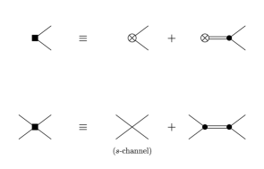
Figure 1: Effective vertices contributing to vector transitions in the s–channel. The crossed circle stands for an external vector current insertion. A double line indicates the $\rho$ and single ones the pseudoscalars. Local vertices on the right–hand side are provided, at leading order, by ${\cal L}^{(2)}_{\chi}$.

The construction of these vertices goes as sketched in Figure 1 where, at the leading order, the local vertices on the right–hand side of the equivalence are provided by the ${\cal O}(p^{2})$ chiral Lagrangian ${\cal L}_{\chi}^{(2)}$ in Eq. (5). The diagrams contributing to physical observables will be constructed taking into account all possible combinations of these two effective vertices.

We propose to define the spin–1 meson width as the imaginary part of the pole generated by resumming those diagrams, with an absorptive part in the s–channel, that contribute to the two–point function of the corresponding vector current. That is, the pole of

$$\Pi_{\mu\nu}^{jk}\,=\,i\,\int\,d^{4}x\,e^{iqx}\,\langle 0|\,T(V_{\mu}^{j}(x)V_{\nu}^{k}(0))\,|0\rangle\;,$$ (10)

with

$$V_{\mu}^{j}\,=\,\frac{\displaystyle\delta S_{\chi V}}{\displaystyle\delta v_{j}^{\mu}}\;,$$ (11)

with $S_{\chi V}$ the action associated to ${\cal L}_{\chi V}$. We take the $\rho^{0}$ quantum numbers that correspond to $j=k=3$. Lorentz covariance and current conservation allow us to define an invariant function of $q^{2}$ through

$$\Pi_{\mu\nu}^{33}\, = \,(q^{2}g_{\mu\nu}\,-\,q_{\mu}q_{\nu})\,\Pi^{\rho}(q^{2})\;,$$

(12)

$$\Pi^{\rho}(q^{2})\, = \,\Pi_{(0)}^{\rho}\,+\,\Pi_{(1)}^{\rho}\,+\,\Pi_{(2)}^{\rho}\,+\cdots\;,$$

where $\Pi_{(0)}^{\rho}$ corresponds to the tree level contribution, $\Pi_{(1)}^{\rho}$ to the one–loop amplitudes and so forth. By evaluating those diagrams in Figure 2 we find

$$\Pi^{\rho}(q^{2})\, = \,\frac{\displaystyle F_{V}^{2}}{\displaystyle M_{V}^{2}-q^{2}}\,\left[1+\omega\sum_{n=0}^{\infty}\,\left(\,\frac{\displaystyle q^{2}}{\displaystyle M_{V}^{2}}\,\omega\right)^{n}\right]\;,$$

$$\omega\, = \,-\,\frac{\displaystyle M_{V}^{2}}{\displaystyle F_{V}^{2}}\,\frac{\displaystyle M_{V}^{2}}{\displaystyle M_{V}^{2}-q^{2}}\,4\,\overline{B_{22}}\;,$$ (13)

where $\overline{B_{22}}$ has been defined properly in Ref. [17].

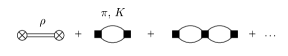
Figure 2: Dyson–Schwinger resummation giving $\Pi^{\rho}(q^{2})$. The effective squared vertices are those given in Figure 1.

Now, resumming, using that $F_{V}^{2}=2F^{2}$ (see Eq. (9)), we get for the imaginary part of the pole

$$M_{V}\Gamma_{\rho}(q^{2})\, = \,-\,2M_{V}^{2}\,\frac{\displaystyle q^{2}}{\displaystyle F^{2}}\,\mbox{Im}\,\overline{B_{22}}$$

$$= \frac{\displaystyle M_{V}^{2}\,q^{2}}{\displaystyle 96\,\pi\,F^{2}}\,\biggl{[}\,\sigma_{\pi}^{3}\,\theta(q^{2}-4m_{\pi}^{2})\,\biggr{.}$$ (14)

$$\;\;\;\;\;\left.+\frac{\displaystyle 1}{\displaystyle 2}\sigma_{K}^{3}\,\theta(q^{2}-4m_{K}^{2})\right]\,,$$

where $\sigma_{P}\,=\,\sqrt{1-4m_{P}^{2}/q^{2}}$. In Ref. [17] it is shown that this result is independent of the spin–1 field formulation that has been chosen. We emphasize that our result for $\Gamma_{\rho}(q^{2})$ is constrained by chiral symmetry and the asymptotic behaviour of $\mbox{Im}\,\Pi^{\rho}(q^{2})$ ruled by QCD. It would be demanding to have a different, leading, off–shell behaviour without spoiling those all–important features.

A similar procedure could be applied to higher multiplicity intermediate states by constructing the relevant effective vertices analogous to those in Figure 1. Although technically much more involved, its study would be necessary to evaluate the width of other resonances such as the $\omega$(872) or the axial–vector mesons.

4 Vector form factor of the pion

The pion vector form factor, $F_{V}(s)$ is defined through

$$\langle\,\pi^{+}(p^{\prime})\,\pi^{-}(p)\,|\,V_{\mu}^{3}\,|\,0\,\rangle\,=\,(p-p^{\prime})_{\mu}\,F_{V}(s)\;,$$ (15)

where $s=q^{2}=(p+p^{\prime})^{2}$ and $V_{\mu}^{3}$ is the third component of the vector current associated to the $SU(3)$ flavour symmetry of the QCD Lagrangian. This form factor drives the hadronic part of both $e^{+}e^{-}\rightarrow\pi^{+}\pi^{-}$ and $\tau^{-}\rightarrow\pi^{-}\pi^{0}\nu_{\tau}$ processes in the isospin limit. At very low energies, $F_{V}(s)$ has been studied in the $\chi$PT framework up to ${\cal O}(p^{6})$ [19, 20]. A successful study at the $\rho(770)$ energy scale has been carried out in the resonance chiral theory in Ref. [16].

Analyticity and unitarity properties of $F_{V}(s)$ tightly constrain, on general grounds, the structure of the form factor [16, 21]. Elastic unitarity and Watson final–state theorem relate the imaginary part of $F_{V}(s)$ to the partial wave amplitude $t_{1}^{1}$ for $\pi\pi$ elastic scattering, with angular momentum and isospin equal to one, as

$$\mbox{Im}\,F_{V}(s+i\varepsilon)\,=\;e^{i\delta_{1}^{1}}\,\sin(\delta_{1}^{1})\,F_{V}(s)^{*}\,,$$ (16)

that shows that the phase of $F_{V}(s)$ must be $\delta_{1}^{1}$. Thus analyticity and unitarity properties of the form factor are accomplished by demanding that it should satisfy a n–subtracted dispersion relation with the Omnès solution [16, 22]

$$F_{V}(s) = \exp\left\{\sum_{k=0}^{n-1}\frac{\displaystyle s^{k}}{\displaystyle k!}\frac{\displaystyle d^{k}}{\displaystyle ds^{k}}\ln F_{V}(s)|_{s=0}\;\right.$$ (17)

$$\;\;\;\;\;\;\;\left.+\,\frac{\displaystyle s^{n}}{\displaystyle\pi}\int_{4m_{\pi}^{2}}^{\infty}\frac{\displaystyle dz}{\displaystyle z^{n}}\frac{\displaystyle\delta_{1}^{1}(z)}{\displaystyle z-s-i\varepsilon}\right\}.$$

This solution is strictly valid only below the inelastic threshold ($s<16m_{\pi}^{2}$), however higher multiplicity intermediate states are suppressed by phase space and ordinary chiral counting. The $\delta_{1}^{1}(s)$ phase–shift, appearing in Eq. (17), is rather well known, experimentally, up to $E\sim 2\,\mbox{GeV}$ [23].

Therefore and with an appropriate number of subtractions we can parameterize $F_{V}(s)$ with the subtraction constants appearing in the first term of the exponential in Eq. (17). In Ref. [21] we have used three subtractions :

$$F_{V}(s) = \exp\left\{\alpha_{1}s\,+\,\frac{\displaystyle 1}{\displaystyle 2}\alpha_{2}s^{2}\,\right.$$ (18)

$$\;\;\;\;\;\;+\left.\frac{\displaystyle s^{3}}{\displaystyle\pi}\int_{4m_{\pi}^{2}}^{\Lambda^{2}}\frac{\displaystyle dz}{\displaystyle z^{3}}\frac{\displaystyle\delta_{1}^{1}(z)}{\displaystyle z-s-i\varepsilon}\,\right\},$$

where we have introduced an upper cut in the integration, $\Lambda$. This cut–off has to be taken high enough not to spoil the, a priori, infinite interval of integration, but low enough that the integrand is well known in the interval. The two subtraction constants $\alpha_{1}$ and $\alpha_{2}$ (a third one is fixed by the normalization $F_{V}(0)=1$) are related with the squared charge radius of the pion $\langle r^{2}\rangle_{V}^{\pi}$ and the quadratic term $c_{V}^{\pi}$ in the low–energy expansion

$$F_{V}(s)\,=\,1+\frac{\displaystyle 1}{\displaystyle 6}\langle r^{2}\rangle_{V}^{\pi}s\,+\,c_{V}^{\pi}s^{2}\,+\,{\cal O}(s^{3}),$$ (19)

through the relations

$$\langle r^{2}\rangle_{V}^{\pi} = 6\,\alpha_{1}\;,$$

$$c_{V}^{\pi} = \frac{\displaystyle 1}{\displaystyle 2}(\alpha_{2}+\alpha_{1}^{2})\,.$$ (20)

$F_{V}(s)$ endows the hadronic dynamics in the $\tau^{-}\rightarrow\pi^{-}\pi^{0}\nu_{\tau}$ decay. This process has recently been measured accurately by three experimental groups [2] : ALEPH, CLEO-II and OPAL. We have taken $F_{V}(s)$, as given by Eq. (18), to fit the ALEPH set of data. The input of the $\delta_{1}^{1}(s)$ phase–shift is included as follows [21]. Resonance chiral theory and vector meson dominance provide a model–independent analytic expression that describes properly the $\rho(770)$ contribution [16]

$$\delta_{1}^{1}(s)\,=\,\arctan\left\{\frac{\displaystyle M_{\rho}\Gamma_{\rho}(s)}{\displaystyle M_{\rho}^{2}-s}\right\}\,,$$ (21)

with $\Gamma_{\rho}(s)$ the off–shell $\rho(770)$ width in Eq. (14). This phase–shift is accurate up to $E\sim 1\,\mbox{GeV}$. At higher energies heavier resonances with the same quantum numbers pop up and we use the available experimental data from Ochs [23]. However there are still contributions that are not taken into account with Ochs data. These are those of coupled channels that open at the $K\overline{K}$ threshold [24]. Therefore in order to have a conservative determination of the observables we choose to fit the ALEPH data up to $\sqrt{s}\simeq 1.1\,\mbox{GeV}$ where we have a thorough control of the contributions. We obtain, using Eq. (20),

$$M_{\rho} = (0.775\,\pm\,0.001)\,\mbox{GeV},$$

$$\langle r^{2}\rangle_{V}^{\pi} = (11.04\,\pm\,0.12)\,\mbox{GeV}^{-2},$$ (22)

$$c_{V}^{\pi} = (3.78\,\pm\,0.04)\,\mbox{GeV}^{-4},$$

with $\chi^{2}/d.o.f.=33.8/21$. In Figures 3 and 4 we show the prescription of $F_{V}(s)$ as given by Eq. (18) with the results of the fit (Eq. (22)).

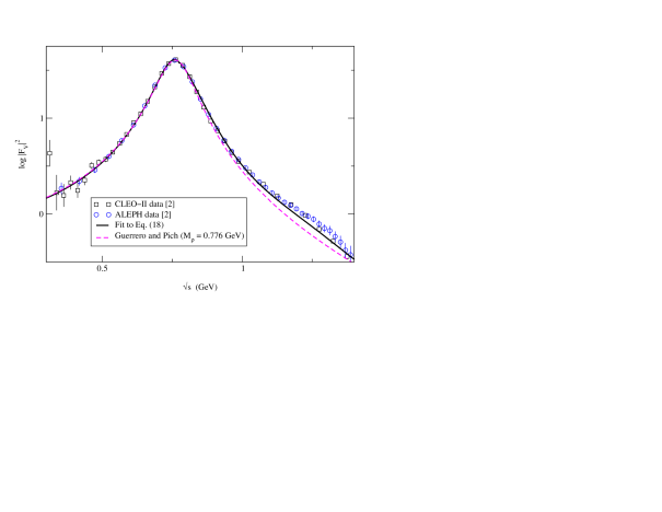
Figure 3: Comparison of experimental data of $\tau$ decays with the results of our fit (Eq. (18)) and the prediction of the Guerrero and Pich form factor (Eq. (28)).

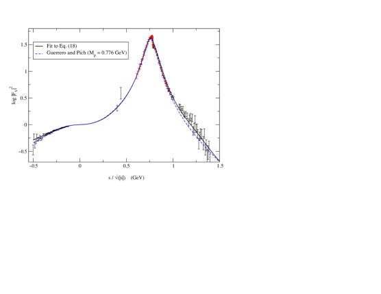
Figure 4: Comparison of experimental data of $e^{+}e^{-}$ (time–like) [25] and $e\pi$ (space–like) [26] with the results of our fit to $\tau$ data (Eq. (18)) and the prediction of the Guerrero and Pich form factor (Eq. (28)).

A different model–independent procedure was followed in Ref. [16] where $F_{V}(s)$ was compelled by further requirements than those of analyticity and unitarity. The behaviour of the vector form factor of the pion, at low energies, is driven by chiral symmetry. The $SU(2)$ result of $\chi$PT up to ${\cal O}(p^{4})$ [19] is

$$F_{V}^{\chi}(s)=1+\frac{\displaystyle 2L_{9}^{r}(\mu)}{\displaystyle F^{2}}s-\frac{\displaystyle s}{\displaystyle 96\pi^{2}F^{2}}A\left(\frac{\displaystyle m_{\pi}^{2}}{\displaystyle s},\frac{\displaystyle m_{\pi}^{2}}{\displaystyle\mu^{2}}\right),$$ (23)

where $L_{9}$ is an, a priori unknown, coupling from the ${\cal O}(p^{4})$ $\chi$PT Lagrangian, and $A(x,y)=\ln y+8x-5/3+\sigma_{x}^{3}\ln((\sigma_{x}+1)/(\sigma_{x}-1))$, $\sigma_{x}=\sqrt{1-4x}$, the two–point one–loop integral containing the chiral logarithms. Alternatively one could consider the evaluation of $F_{V}(s)$ in the leading large $N_{C}$ limit where the vector form factor is given by an infinite set of resonant contributions. Considering only the $\rho(770)$ contribution we have [18]

$$F_{V}^{N_{C}}(s)=\frac{\displaystyle M_{\rho}^{2}}{\displaystyle M_{\rho}^{2}-s}\,.$$ (24)

Guerrero and Pich proceeded by matching both results $F_{V}^{\chi}(s)$ and $F_{V}^{N_{C}}(s)$ . This procedure is simplified because of the fact that the one–loop contribution to $F_{V}^{\chi}(s)$ is next-to-leading in the $1/N_{C}$ expansion. Then we have

$$F_{V}(s)=\frac{\displaystyle M_{\rho}^{2}}{\displaystyle M_{\rho}^{2}-s}-\frac{\displaystyle s}{\displaystyle 96\pi^{2}F^{2}}A\left(\frac{\displaystyle m_{\pi}^{2}}{\displaystyle s},\frac{\displaystyle m_{\pi}^{2}}{\displaystyle M_{\rho}^{2}}\right).$$ (25)

Notice that this result implies a resummation of the polynomial part given by $\chi$PT and prescribes a value for $L_{9}^{r}(M_{\rho})$. The next step was to match this result with the prescription provided by analyticity and unitarity through the Omnès solution (17). This gives

$$F_{V}(s)\!=\!\frac{\displaystyle M_{\rho}^{2}}{\displaystyle M_{\rho}^{2}-s}\exp\left\{\frac{\displaystyle-s}{\displaystyle 96\pi^{2}F^{2}}A\left(\frac{\displaystyle m_{\pi}^{2}}{\displaystyle s},\frac{\displaystyle m_{\pi}^{2}}{\displaystyle M_{\rho}^{2}}\right)\!\right\}.$$ (26)

Finally, noticing that the pion contribution to $\Gamma_{\rho}(s)$ in Eq. (14) can be written too as

$$\Gamma_{\rho}(s)=-\frac{\displaystyle M_{\rho}s}{\displaystyle 96\pi^{2}F^{2}}\,\mbox{Im}\,A\left(\frac{\displaystyle m_{\pi}^{2}}{\displaystyle s},\frac{\displaystyle m_{\pi}^{2}}{\displaystyle M_{\rho}^{2}}\right),$$ (27)

Guerrero and Pich moved this piece from the exponential to the pole, with the final result

$$F_{V}(s)\!\! \!=\!\!\! \!\frac{\displaystyle M_{\rho}^{2}}{\displaystyle M_{\rho}^{2}-s-iM_{\rho}\Gamma_{\rho}(s)}\times$$ (28)

$$\!\!\exp\left\{\frac{\displaystyle-s}{\displaystyle 96\pi^{2}F^{2}}\mbox{Re}A\left(\frac{\displaystyle m_{\pi}^{2}}{\displaystyle s},\frac{\displaystyle m_{\pi}^{2}}{\displaystyle M_{\rho}^{2}}\right)\!\right\}.$$

Note that the only free parameter in this expression is $M_{\rho}$. In spite of including the $\rho(770)$ resonance only, and as can be seen in Figures 3 and 4, it does an excellent job in describing experimental data up to $E\sim 1\,\mbox{GeV}$, showing, once again, the compelling role of chiral symmetry, vector meson dominance, analyticity and unitarity in the description of form factors.

5 $\tau^{-}\rightarrow(3\pi)^{-}\nu_{\tau}$ : axial–vector form factors

Similar ideas to the ones proposed previously can be applied to more complicated processes. In $\tau^{-}\rightarrow(\pi\pi\pi)^{-}\nu_{\tau}$ the hadronic matrix element has, in the isospin limit, contribution from the corresponding axial–vector current ($A_{\mu}^{-}$) only. These form factors can be defined as

$$\!\!\!\!\!\!\!\!\!\!\!\!\!\!\!\!\!\!\!\!\!\!\!\!\!\!\!\!\!\!\!\!\!\!\!\!\!\!\!\langle\,\pi^{-}(p_{1})\,\pi^{-}(p_{2})\,\pi^{+}(p_{3})\,|A_{\mu}^{-}|\,0\,\rangle\,=$$

$$\left(g_{\mu\nu}-\frac{\displaystyle Q_{\mu}Q_{\nu}}{\displaystyle Q^{2}}\right)\,\left[\,F_{1}(Q^{2},s_{1},s_{2})\,(p_{1}-p_{3})^{\nu}\right.$$

$$+\,\left.F_{1}(Q^{2},s_{2},s_{1})\,(p_{2}-p_{3})^{\nu}\,\right]\mbox{$\!\!\!\!\!\!\!\!$}$$

$$\;\;\;\;+\,F_{2}(Q^{2},s_{1},s_{2})\,Q_{\mu}\,,$$ (29)

where $Q=p_{1}+p_{2}+p_{3}$, $s_{i}=(Q-p_{i})^{2}$. In the chiral limit ($m_{\pi}=0$) $F_{2}(Q^{2},s_{1},s_{2})=0$ and we have just one form factor $F_{1}(Q^{2},s_{1},s_{2})$ to work out. This form factor is driven by both vector and axial–vector resonances.

A thorough analysis of $F_{1}(Q^{2},s_{1},s_{2})$ in the model–independent framework of resonance chiral theory and vector meson dominance is under way [27]. Let us just to point out here the necessity of this study. As we said in the Introduction the present sets of experimental data are analysed using the TAUOLA library where the Kühn and Santamaria [5] hadronic matrix elements are implemented. This model was constructed to be consistent with $\chi$PT at the leading ${\cal O}(p^{2})$ order and with the asymptotic behaviour that QCD demands to form factors. At ${\cal O}(p^{4})$ in $\chi$PT the contribution of spin–1 resonances appears, and the low–energy behaviour of $F_{1}(Q^{2},s_{1},s_{2})$ given by the model is

$$F_{1}^{KS}\,\simeq\,1\,+\,\frac{\displaystyle s_{1}}{\displaystyle M_{V}^{2}}\,+\,\frac{\displaystyle Q^{2}}{\displaystyle M_{A}^{2}}\,+\,{\cal O}\left(\frac{\displaystyle q^{4}}{\displaystyle M_{R}^{4}}\right)\,,$$ (30)

where $M_{V}$ and $M_{A}$ are masses of vector and axial–vector resonances, respectively. However the evaluation of the form factor within resonance chiral theory [27] provides the low–energy expansion result

$$F_{1}^{\chi}\,\simeq\,1\,+\,\frac{\displaystyle 3}{\displaystyle 2}\,\frac{\displaystyle s_{1}}{\displaystyle M_{V}^{2}}\,+\,(\ldots)\,+\,{\cal O}\left(\frac{\displaystyle q^{4}}{\displaystyle M_{R}^{4}}\right)\,,$$ (31)

in agreement with the evaluation within the framework of $\chi$PT at ${\cal O}(p^{4})$ [28]. This shows that the Kühn and Santamaria model is no longer consistent, at ${\cal O}(p^{4})$, with the chiral symmetry of QCD and, therefore, further studies are required.
Acknowledgements
I wish to thank D. Gómez Dumm and A. Pich for a fruitful and demanding collaboration, and to R.J. Sobie and J.M. Roney for the luxurious organization of the Tau2000 meeting. I thank also A. Pich for a critical reading of the text. This work has been partially supported by CICYT PB97–1261.

References

- [1] A. Weinstein, these proceedings; R. Sobie, these proceedings; J. Van Eldik, these proceedings.
- [2] R. Barate et al, ALEPH Col., Z. Phys. C76 (1997) 15; S. Anderson et al , CLEO Col., Phys. Rev. D61 (2000) 112002; K. Ackerstaff et al, OPAL Col., Eur. Phys. J. C7 (1999) 571.
- [3] D.M. Asner et al, CLEO-II Col., Phys. Rev. D61 (1999) 012002; K. Ackerstaff, OPAL Col., Z. Phys. C75 (1997) 593; R. Barate et al, ALEPH Col., Eur. Phys. J. C4 (1998) 409; P. Abreu et al, DELPHI Col., Phys. Lett. 426 (1998) 411.
- [4] R. Decker, S. Jadach, M. Jezabek, J.H. Kühn and Z. Was, Comput. Phys. Commun. 76 (1993) 361; ibid. 70 (1992) 69; ibid. 64 (1990) 275.
- [5] J.H. Kühn and A. Santamaria, Z. Phys. C48 (1990) 445.
- [6] G.J. Gounaris and J.J. Sakurai, Phys. Rev. Lett. 21 (1968) 244.
- [7] S. Weinberg, Physica 96A (1979) 327.
- [8] H. Leutwyler, Annals of Physics 235 (1994) 165.
- [9] J. Schwinger, Phys. Lett. B24 (1967) 473.
- [10] S. Weinberg, Phys. Rev. 166 (1968) 1568.
- [11] J. Gasser and H. Leutwyler, Ann. of Phys. (NY) 158 (1984) 142; J. Gasser and H. Leutwyler, Nucl. Phys. B250 (1985) 465.
- [12] S. Coleman and E. Witten, Phys. Rev. Lett. 45 (1980) 100.
- [13] G. Ecker, J. Gasser, A. Pich and E. de Rafael, Nucl. Phys. B321 (1989) 311.
- [14] D. Espriu, E. de Rafael and J. Taron, Nucl. Phys. B345 (1990) 22.
- [15] G. Ecker, Prog. Part. Nucl. Phys. 35 (1995) 1; A. Pich, Rep. Prog. Phys. 58 (1995) 563.
- [16] F. Guerrero and A. Pich, Phys. Lett. B412 (1997) 382.
- [17] D. Gómez Dumm, A. Pich and J. Portolés, Phys. Rev. D62 (2000) 054014.
- [18] G. Ecker, J. Gasser, H. Leutwyler, A. Pich and E. de Rafael, Phys. Lett. B223 (1989) 425.
- [19] J. Gasser and H. Leutwyler, Nucl. Phys. B250 (1985) 517.
- [20] J. Bijnens, G. Colangelo and P. Talavera, J. High Energy Physics, 05 (1998) 014.
- [21] A. Pich and J. Portolés, work in progress.
- [22] N.I. Muskhelishvili, Singular integral equations, Noordhof, Groningen, 1953; R. Omnès, Nuovo Cimento, 8 (1958) 316.
- [23] W. Ochs, Univ. of Munich thesis (1973).
- [24] J.A. Oller, E. Oset, J.E. Palomar, hep-ph/0011096.
- [25] Barkov et al., Nucl. Phys. B256 (1985) 365.
- [26] Amendolia et al. Nucl. Phys. B277 (1986) 168.
- [27] D. Gómez Dumm, A. Pich and J. Portolés, work in progress.
- [28] G. Colangelo, M. Finkemeier and R. Urech, Phys. Rev. D54 (1996) 4403.