November 2000 FERMILAB-Pub-00/284-T OUTP-00-39P SUSX-TH/00-018 UFIFT-HET00-27
Neutrino Masses and Mixing in Brane-World Theories

Abstract

We present a comprehensive study of five-dimensional brane-world models for neutrino physics based on flat compactifications. Particular emphasis is put on the inclusion of bulk mass terms. We derive a number of general results for such brane-world models with bulk mass terms. In particular, in the limit of small brane-bulk couplings, the electroweak eigenstates are predominantly given as a superposition of three light states with non-trivial small admixtures of bulk states. As a consequence, neutrinos can undergo standard oscillations as well as oscillation into bulk Kaluza-Klein states. We use this structure to construct a specific model based on $\mathbb{Z}_{2}$ orbifolding and bulk Majorana masses which is compatible with all observed oscillation phenomena. The solar neutrino deficit is explained by oscillations into sterile bulk states while the atmospheric neutrino deficit is due to $\nu_{\mu}$ – $\nu_{\tau}$ oscillations with naturally maximal mixing. In addition, the model can accommodate the LSND result and a significant neutrino dark matter component. We also analyze the constraints from supernova energy loss on neutrino brane-world theories and show that our specific model is consistent with these constraints.

1 Introduction

Two recent ideas, namely the brane-world idea [1, 2, 3, 4, 5, 6, 7, 8] and the possibility of having large gravitation-only additional dimensions [2, 9, 6, 7], may significantly change the relation between string- or M-theory and low-energy particle physics. Not only do these ideas motivate new directions in particle physics model building but they also provide new generic structures within string theory which may be experimentally testable. In this context, an important role is played by bulk particles coupling to standard model particles only gravitationally. Particularly relevant are the Kaluza-Klein modes of the higher-dimensional graviton [6] and higher-dimensional bulk fermions. In this paper, we focus on the latter possibility of bulk fermions. They provide candidates for right-handed neutrinos and might, therefore, play an important role in neutrinos physics.

The potential relevance of these particles for neutrino physics has first been first pointed out and analyzed in Ref. [10, 11, 12]. Phenomenological analysis have been performed in [13]–[26]. The importance of bulk masses has been pointed out in [20], where an explicit 6-dimensional example with Dirac bulk masses has been presented. The phenomenological implications of a five-dimensional brane-world model with bulk Dirac-masses for solar, atmospheric, short-baseline and supernova oscillations have been studied in [22].

The main goal of this paper is to present a comprehensive phenomenological study of five-dimensional brane-world models for neutrino mass and mixing. Particular emphasis will be put on the model-building options that arise from the various types of bulk mass terms. We will focus on compactifications on a flat metric as well as on bulk mass terms without any explicit dependence on the additional coordinate. Furthermore, we assume that all right-handed neutrinos propagate in the fifth dimension. Within this general setting we will present a number of exact results for the mass spectrum as well as the mixing angles. Furthermore, based on these general results, we will give an explicit example based on the orbifold $S^{1}/\mathbb{Z}_{2}$ and Majorana bulk-masses related to the $S^{1}$ model with Dirac masses studied in Ref. [22]. As we will see, this model is consistent with the oscillation data presently available. In particular, we show that the solar neutrino deficit can be explained by small-mixing angle oscillations of $\nu_{e}$ into a tower of sterile neutrinos. Unlike such oscillations into a single sterile neutrino this option is not disfavored by the recent SuperKamiokande results. In addition, the model naturally leads to a maximal mixing angle in the $\nu_{\mu}$ – $\nu_{\tau}$ sector and can explain the atmospheric neutrino results. At the same time it contains two neutrinos in the eV range that can provide a cosmologically significant source of dark matter. It also has room to accommodate the LSND signal and in general predicts $\nu_{e}\leftrightarrow\nu_{\mu}$ oscillations with ${\Delta m^{2}_{\text{}}}>{\Delta m^{2}_{\text{ATM}}}$ and a small amplitude. The alternative model-building option, namely large mixing angles between standard and sterile Kaluza-Klein neutrinos, is disfavored by the requirement of not having significant departures from Standard Model processes [18]. In particular, this disfavors the possibility that sterile bulk states play a significant role in atmosperic neutrino oscillations.

In the context of string- and M-theory, bulk fermions arise as superpartners of gravitational moduli, such as, for example, radii of internal spaces. Given this origin, the existence of bulk fermions is practically unavoidable in any supersymmetric string compactification and, therefore, represents a quite generic feature of string theory. This, in our opinion, constitutes the most likely origin of such particles within a fundamental theory and, at the same time, provides the best theoretical motivation to study brane-world neutrino physics. In the context of four-dimensional effective actions from string theory, modulini as candidates for right-handed neutrinos have been proposed in Ref. [27]. The phenomenological relevance of such bulk fermions for neutrino physics is basically controlled by three different features of the theory. Specifically, these are the masses of the bulk fermions, the radii of the additional dimensions and the size of the brane-bulk coupling between bulk fermions and standard model neutrinos. Let us discuss these three features and their relation to string- and M-theory separately.

So far, brane-world model building in the context of neutrino physics has been mostly focusing on exactly massless bulk fermions (see, however, Ref. [10, 15] where bulk mass terms have been considered). However, bulk mass terms constitute an important model-building option which should be taken into consideration. In fact, unless forbidden by specific symmetries, bulk mass terms should not be ignored. Of course, bulk fermions can be candidates for sterile neutrinos only if these masses are sufficiently small . One should, therefore, worry about the origin of such small mass scales. Within perturbative string theory, moduli fields constitute flat directions and, consequently, have vanishing mass. The same is true for their fermionic superpartners as long as supersymmetry is unbroken. String theory, therefore, provides a generic reason why bulk fermion masses may be much smaller than the string scale. Eventually, non-perturbative effects have to be taken into account in order to break supersymmetry and stabilize the moduli fields. Those will generate masses for the moduli field and, most likely, masses for the bulk fermions as well. Hence, the inclusion of small bulk fermion masses is quite well motivated from the viewpoint of string theory. It is one of the central points of this paper, to take this insight seriously and include the most general structure of bulk mass terms into our analysis.

The specific size of these mass terms as well as the size of the additional dimension depend on non-perturbative effects and are largely uncertain from a theoretical perspective. Therefore, in the general part of the paper, we will not focus on any specific choice for these scales. Of course, the tower of bulk fermions will only be directly relevant for oscillations if the bulk masses and the scale of the additional dimension are sufficiently small. For the explicit example we will focus on such a case with small bulk masses and a large fifth dimension close to the experimental upper bound.

Finally, we should address the possible origin of the brane-bulk mass terms mixing bulk fermions and standard neutrinos. In fact, such couplings may arise quite generically, for example, in the context of Horava-Witten theory [1]. In the 11-dimensional formulation of this theory, the 10-dimensional Yang-Mills theories on the boundaries contain terms bilinear in the gravitino (giving rise to bulk fermions in lower dimensions) and the gauginos (giving rise to the standard model fermions). These are precisely the terms needed to generate the desired brane-bulk mixing. From the perspective of effective four-dimensional supergravity theories such terms can be understood as arising from higher-dimensional non-renormalizable operators involving moduli and standard model fields with appropriate VEVs inserted. It would certainly be interesting to analyze this in more detail. However, for the purpose of the present paper, we content ourselves with these general remarks.

We would like to point out that there exist models, particularly in the context of string compactifications, where, in addition to bulk right-handed neutrinos, one also has right-handed neutrinos on the brane. Such models are problematic for values of the fundamental scale far below the GUT scale. This is because a see-saw mechanism on the brane, with the right-handed neutrino masses being set by this low fundamental scale, will typically not suppress the associated contribution to the left-handed neutrino masses enough. In this paper, we will not consider models with such singlet neutrino states on the brane.

In the next Section we present the general structure of the five-dimensional brane-world model along with the associated four-dimensional effective action. The Section concludes with a discussion of the various symmetries that can be imposed on this brane-world theory for model-building purposes. The spinor properties used in this Section are summarized in Appendix A. Section 3 contains a general analysis of the structure of masses and mixing and a discussion of the various resulting model building options. This discussion is mainly based on a perturbative diagonalization of the mass matrix assuming small brane-bulk mixing. The Section is complemented by Appendix B which contains some of the more technical aspects related to the exact diagonalization of the mass matrix. In Section 4 the constraints from energy loss in supernovae are discussed. Section 5 describes a specific model with a bulk Majorana mass which results in a small mixing between electroweak eigenstates and bulk states. It is shown that, in the context of this model, the small-angle MSW solution is a viable solution for the solar neutrino problem. At the same time, the atmospheric oscillation phenomena as well as the LSND signal can be understood.

2 General framework

In this Section, we will set up our formalism and present the general structure of five-dimensional neutrino brane-world models. Subsequently, we perform a Kaluza-Klein reduction to obtain the associated four-dimensional effective theory which will be the starting point for our analysis of neutrino masses and mixing.

2.1 Five-dimensional brane-world models of neutrino physics

We consider brane world theories with a five-dimensional bulk and coordinates denoted by $x^{\alpha}$ where $\alpha,\beta,\cdots=0,1,2,3,4$. Spinors in this five-dimensional bulk theory provide candidates for right-handed neutrinos and are, therefore, of particular importance in our context. As mentioned above, within the framework of string- or M-theory compactifications the presence of such bulk spinors is practically unavoidable, since they arise as superpartners of moduli fields. We assume the existence of an arbitrary number, $N$, of bulk Dirac spinors  $\Psi_{I}$ where $I,J,\cdots=1,\cdots,N$. Given these fields, one might want to write the most general five-dimensional action bilinear in the spinors and respecting five-dimensional Lorentz-invariance. However, there is an important generalization to this that arises from including bulk gauge fields $A_{\alpha}$ under which the fermions are charged. Within string- or M-theory such bulk vector fields arise quite generically as part of five-dimensional vector super-multiplets. Also gauging of the bulk fermions with respect to these vector fields is realized in large classes of models such as the five-dimensional brane-world models originating from heterotic M-theory [4, 5]. Later on, we will compactify the five-dimensional theory on a certain vacuum state to four dimensions. All we really have to require is that this vacuum state respects four-dimensional Lorentz invariance. As a consequence, in such a vacuum state, non-vanishing vacuum expectation values (VEVs) for the components $A_{4}$ of the bulk vector fields in the direction to be compactified are allowed. Hence, we should consider two types of bulk mass terms. First, there are mass terms that respect five-dimensional Lorentz invariance. We can think of such mass terms as being generated by VEVs of bulk scalars. Secondly, there are mass terms generated by VEVs of the components $A_{4}$ of bulk vector fields. They arise once five-dimensional Lorentz invariance is spontaneously broken to four-dimensional Lorentz invariance by the vacuum state. We split the five-dimensional action as

$$S_{5}=S_{\rm bulk}+S_{\rm brane}$$ (2.1)

into a bulk and a brane part. Taking into account the two types of mass terms as discussed, the relevant part of the bulk action is given by

$$S_{\rm bulk} = \int d^{5}x\left[\bar{\Psi}_{I}\gamma^{\alpha}i\partial_{\alpha}\Psi_{I}+\mu^{S}_{IJ}\bar{\Psi}_{I}\Psi_{J}-\frac{1}{2}(M^{S}_{IJ}\bar{\Psi}^{c}_{I}\Psi_{J}+\text{h.c.})\right.$$ (2.2)

$$\left.+i\mu^{V}_{IJ}\bar{\Psi}_{I}\gamma_{5}\Psi_{J}-\frac{1}{2}(M^{V}_{IJ}\bar{\Psi}^{c}_{I}\gamma_{5}\Psi_{J}+\text{h.c.})\right]\;.$$

Here, $\mu_{S}$ and $M_{S}$ are the Lorentz-invariant Dirac and Majorana mass matrices, respectively. The subscripts “$S$” refer to their possible origin as being generated by VEVs of bulk scalar fields. These mass matrices have two vector-like counterparts, $\mu_{V}$ and $M_{V}$, generated by VEVs of bulk vector fields in the way indicated above . To see in some more detail how this happens, we note that in five dimensions the spinors $\Psi$ and their charge conjugate $\Psi^{c}$ transform in the same way under the five-dimensional Lorentz group. Therefore, in addition to the “ordinary” kinetic terms of the form $\bar{\Psi}\gamma^{\alpha}i\partial_{\alpha}\Psi$, we can also write Majorana kinetic terms of the form $\bar{\Psi}^{c}\gamma^{\alpha}i\partial_{\alpha}\Psi+\text{h.c.}$. In the most general case one should gauge a linear combination of these terms. One can see that with an appropriate redefinition in the $(\Psi,\Psi^{c})$ space the Majorana kinetic term can always be removed. This is why, in the above action, we have only written the standard kinetic term. However, in general, one cannot simultaneously convert the couplings to the vector field to the same standard form. In other words, once the kinetic term is in the canonical form, the gauge transformations can still mix the $\Psi$ and $\Psi^{c}$ fields . Therefore, after taking into account the vector field VEVs, we indeed generate the Dirac and the Majorana vector mass terms given in (2.2). From the structure of the various terms in (2.2) we deduce the following symmetry properties of the associated mass matrices.

$$\mu_{S}={\mu_{S}}^{\dagger}\;,\qquad M_{S}={M_{S}}^{T}\;,\qquad\mu_{V}={\mu_{V}}^{\dagger}\;,\qquad M_{V}={M_{V}}^{T}$$ (2.3)

Are there other sensible generalizations of the bulk action that we have not yet taken into account? In models where the fifth dimension is divided by an orbifolding symmetry one should impose invariance of the action only under those infinitesimal coordinate transformations that are compatible with the orbifolding. Since this may be a smaller set of transformations it leads to generalizations of the action given above. Typically, in these cases, one can allow explicit orbifold-dependent functions such as step-functions in the bulk action. Another way of generating mass terms which effectively depend on the additional dimension is to consider a vacuum state with a non-flat metric. Explicit coordinate dependence of the mass terms generated in these ways might have interesting consequences for the structure of neutrino masses [28]. For example, generically one expects that the Kaluza-Klein part of the mass matrix does not have a block-diagonal structure any more. In this paper, we will not consider this interesting possibility further but we remark that the general formalism for the diagonalization of the mass matrix in Appendix B is equipped to handle even the more general case of a non block-diagonal mass matrix.

Restricting to the case of coordinate-independent mass parameters, the bulk Lagrangian (2.2) constitutes the most general expression compatible with four-dimensional Lorentz invariance and, therefore, contains all possible mass terms. However, we can ask whether we can generate these mass terms by mechanisms different from the ones already mentioned. To do this, we note that the spinors $\Psi_{I}$ transform in the fundamental of $Sp(4)\simeq SO(5)$. A spinor bilinear, therefore, transforms under $Sp(4)$ as

$${\bf 4}\times{\bf 4}={\bf 1}+{\bf 5}+{\bf 10}\;.$$ (2.4)

We have already discussed the coupling to the singlet ${\bf 1}$ and the vector ${\bf 5}$ leading to the scalar and vector masses, respectively. In addition, there can be a coupling to a second-rank antisymmetric tensor field transforming in the representation ${\bf 10}$. However, only the components of this antisymmetric tensor field pointing into the internal space can take VEVs if we are to preserve four-dimensional Lorentz invariance. Clearly, for the case of one additional dimension these components must vanish by antisymmetry of the tensor field. Therefore, mass terms are generated by VEVs of scalar and vector fields only.

Next, we should set up the brane action. We choose $x^{\mu}$, where $\mu,\nu,\cdots=0,1,2,3$ as the coordinates longitudinal to the brane and $y\equiv x^{4}$ as the transverse coordinate. Furthermore, we locate the brane at $y=0$. The essential fields on the brane that we need to consider for our purpose are the left-handed lepton doublets $L_{i}$, where $i=e,\mu,\tau$ and the relevant Higgs field $H$. As mentioned in the introduction, we will not consider singlet neutrino fields on the brane. We write the lepton doublets in a basis in family space where the charged lepton mass matrix is diagonal and positive. The most general brane-bulk Yukawa couplings invariant under the standard model group can then be written as

$$S_{\rm brane}=\int_{\{y=0\}}d^{4}x\left[-\frac{h_{Ii}}{\sqrt{M_{5}}}\bar{\Psi}_{I}L_{i}H-\frac{h^{c}_{Ii}}{\sqrt{M_{5}}}\bar{\Psi}^{c}_{I}L_{i}H+\text{h.c.}\right]\;.$$ (2.5)

Since the bulk spinors with the normalization fixed by the bulk action (2.2) have mass dimension two, these couplings are suppressed by the square root of a mass scale $M_{5}$ defined by

$$2\pi RM_{5}=\left(\frac{M_{\rm Pl}}{M_{*}}\right)^{2}$$ (2.6)

where $M_{*}$ is the string scale. Furthermore, $R$ is the radius of the circle on which we compactify the fifth dimension transverse to the brane in preparation for our reduction to four dimensions. Also, we restrict the range of the corresponding coordinate as $y\in[-\pi R,\pi R]$ with the endpoints identified.

As mentioned in the introduction, in the context of string- or M-theory, brane-bulk couplings may arise from higher-dimensional gravity-induced operators after inserting appropriate VEVs. From a theoretical viewpoint, their magnitude is rather uncertain and is, in our case, parameterized by the dimensionless couplings $h_{Ii}$ and $h^{c}_{Ii}$. In the context of string theory, we have, of course in mind that our five-dimensional model is obtained by compactification of the ten (or eleven) dimensional theory on a five- (or six-) dimensional internal space with radii of compactification smaller than $R$. In the simple case in which all those internal radii are equal and given by $\rho$, the quantities $R$, $\rho$ and the string scale $M_{*}$ are related by

$$16\pi(2\pi RM_{*})(2\pi\rho M_{*})^{5}=\left(\frac{M_{\rm Pl}}{M_{*}}\right)^{2}\;.$$ (2.7)

From this relation, in models with a low string scale $M_{*}$, we will need $\rho^{-1}$ to be smaller than the string scale in order to get the correct value for the low-energy Planck scale. In such cases, the five-dimensional action specified by eq. (2.1) should be considered as an effective theory below $\rho^{-1}$ (rather than below $M_{*}$). This also means  that we should restrict bulk masses to be smaller than $\rho^{-1}$.

If the bulk fermions propagate in all ten dimensions, as is suggested by their possible interpretation as modulini, then, from eq. (2.6), the dimensionless couplings $h_{Ii}$ and $h^{c}_{Ii}$ are simply given by their ten-dimensional counterparts. On the other hand, if the bulk fermions propagate only in $\delta$ of the ten space-time dimensions (where $5\leq\delta<10$) the couplings $h$ are given by $h=h_{\delta}(2\pi\rho M_{*})^{(10-\delta)/2}$.

2.2 The four-dimensional effective action

We would now like to reduce the above five-dimensional theory and calculate the associated effective four-dimensional action. We require the bulk fields to be periodic on the circle , that is

$$\Psi_{I}(-\pi R)=\Psi_{I}(\pi R)\;.$$ (2.8)

Correspondingly, the bulk fermions can be expanded into Kaluza-Klein modes as

$$\Psi_{I}(x,y)=\frac{1}{\sqrt{2\pi R}}\sum_{n\in\mathbb{Z}}\Psi_{nI}(x)\exp\left(\frac{iny}{R}\right)\;.$$ (2.9)

In addition, it is useful to express each of the modes $\Psi_{nI}$ in terms of two four-dimensional (left-handed) Weyl spinors $\xi_{-nI}$, $\eta_{nI}$ as

$$\Psi_{nI}=\begin{pmatrix}\bar{\xi}_{-nI}\\ \eta_{nI}\end{pmatrix}\;.$$ (2.10)

Here the conjugate $\bar{\xi}$ of a Weyl spinor $\xi$ is defined as $\bar{\xi}=\epsilon\xi^{*}$ where $\epsilon$ is the two-dimensional epsilon symbol. For further details of our conventions we refer to Appendix A. The four-dimensional effective action associated to the brane-world theory (2.1), (2.2), (2.5) is then given by

$${\cal L}={\cal L}_{\rm kin}+{\cal L}_{\rm mass}$$ (2.11)

where the kinetic terms of the bulk fields read

$${\cal L}_{\rm kin}=\sum_{n\in\mathbb{Z}}\left[\eta^{\dagger}_{nI}\sigma^{\mu}i\partial_{\mu}\eta_{nI}+\xi^{\dagger}_{nI}\sigma^{\mu}i\partial_{\mu}\xi_{nI}\right]\;.$$ (2.12)

The all-important mass part of the Lagrangian can be conveniently written in the form

$${\cal L}_{\rm mass}=-\sum_{n\in\mathbb{Z}}\left[\frac{1}{2}\begin{pmatrix}\eta_{n}^{T}&\xi_{n}^{T}\end{pmatrix}{\cal M}_{n}\begin{pmatrix}\eta_{-n}\\ \xi_{-n}\end{pmatrix}+\begin{pmatrix}\eta_{n}^{T}&\xi_{n}^{T}\end{pmatrix}{\cal N}\nu\right]+\text{h.c.}$$ (2.13)

where, for ease of notation, we have adopted a vector notation in family space. That is, for example, $\eta_{n}=(\eta_{n1},\cdots,\eta_{nN})^{T}$ and $\nu=(\nu_{e},\nu_{\mu},\nu_{\tau})^{T}$. Given our conventions for Weyl mass terms in Appendix A, here, the transpose $T$ refers to family space only. Written in block-form, the mass matrix ${\cal M}_{n}$ for the Kaluza-Klein modes at level $n$ takes the form

$${\cal M}_{n}=\begin{pmatrix}M_{1}&\mu^{T}-\frac{in}{R}\\ \mu+\frac{in}{R}&M_{2}\end{pmatrix}\;.$$ (2.14)

Here $M_{1}$ and $M_{2}$ are Majorana mass-matrices related to the scalar and vector Majorana mass-matrices appearing in the five-dimensional bulk action (2.2) by

$$M_{1}=-M_{S}+M_{V}\;,\qquad M_{2}=(M_{S}+M_{V})^{*}\;.$$ (2.15)

The Dirac mass-matrix $\mu$ encodes both scalar and vector Dirac masses and is explicitly defined by

$$\mu=\mu_{S}-i\mu_{V}\;.$$ (2.16)

From eq. (2.3), it is clear that $M_{1}$ and $M_{2}$ are symmetric matrices while, generally, there is no further constraint on $\mu$.

Note that the bulk mass matrices satisfy the relations

$${\cal M}_{-n}={\cal M}_{n}^{T}\;.$$ (2.17)

They ensure that the Majorana mass matrix

$$\qquad\qquad\;\,\begin{array}[]{llllll}\nu^{T}&\eta_{0}^{T}\;\xi_{0}^{T}&\cdots&\eta_{-n}^{T}\;\xi_{-n}^{T}&\eta_{n}^{T}\;\xi_{n}^{T}&\cdots\end{array}$$ (2.19)

$${\cal M} = \begin{array}[]{c}\nu\\ \begin{array}[]{c}\eta_{0}\\ \xi_{0}\end{array}\\ \vdots\\ \begin{array}[]{c}\eta_{-n}\\ \xi_{-n}\end{array}\\ \begin{array}[]{c}\eta_{n}\\ \xi_{n}\end{array}\\ \vdots\end{array}\left(\begin{array}[]{llllll}\phantom{\nu}{0}&\makebox[17.71803pt]{${\cal N}^{T}$}&\cdots&\makebox[22.57399pt]{${\cal N}^{T}$}&\makebox[18.84065pt]{${\cal N}^{T}$}&\cdots\\ \phantom{\begin{array}[]{l}\eta_{0}\\ \xi_{0}\end{array}}{{\cal N}}&\makebox[17.71803pt]{${\cal M}_{0}$}&\cdots&\makebox[22.57399pt]{$0$}&\makebox[18.84065pt]{$0$}&\ldots\\ \vdots&\makebox[17.71803pt]{$\vdots$}&\ddots&\makebox[22.57399pt]{$0$}&\makebox[18.84065pt]{$0$}&\ldots\\ \phantom{\begin{array}[]{c}\eta_{-n}\\ \xi_{-n}\end{array}}{{\cal N}}&\makebox[17.71803pt]{$0$}&0&\makebox[22.57399pt]{$0$}&\makebox[18.84065pt]{${\cal M}_{n}^{T}$}&\\ \phantom{\begin{array}[]{c}\eta_{n}\\ \xi_{n}\end{array}}{{\cal N}}&\makebox[17.71803pt]{$0$}&0&\makebox[22.57399pt]{${\cal M}_{n}$}&\makebox[18.84065pt]{$0$}&\\ \vdots&\makebox[17.71803pt]{$\vdots$}&\vdots&&&\ddots\end{array}\right)$$ (2.50)

associated with the mass Lagrangian (2.11) is indeed symmetric as it should be.

The brane-bulk coupling matrix ${\cal N}$ has the form

$${\cal N}=\begin{pmatrix}m^{c}\\ m\end{pmatrix}\;.$$ (2.51)

The mass matrices $m$ and $m^{c}$ are related to the brane-bulk couplings in the brane action (2.5), respectively and are explicitly given by

$$m_{Ii}=\frac{vh_{Ii}}{\sqrt{2\pi RM_{5}}}=h_{Ii}v\frac{M_{*}}{M_{\rm Pl}}\;,\qquad m^{c}_{Ii}=\frac{vh^{c}_{Ii}}{\sqrt{2\pi RM_{5}}}=h_{Ii}^{c}v\frac{M_{*}}{M_{\rm Pl}}\;.$$ (2.52)

Here $v$ is the Higgs vacuum expectation value.

In what follows we will have occasion to choose the brane-bulk couplings, $h_{Ii}$, to be of a given size for phenomenological reasons. However, there are lower bounds on $M_{*}/h_{Ii}$ at tree level or on $M_{*}/h_{Ii}^{2}$ at one-loop-level by requiring that there be no significant departure from Standard Model processes [18]. It turns out that these constraints can be satisfied within the explicit model to be discussed later. Moreover, it has been suggested that values of $h_{Ii}$ larger than one may be inconsistent with staying in the perturbative domain. However, from eq. (2.7), we see that the string scale is very sensitive to the nature of compactification from higher dimensions so it is always possible to arrange for $h_{Ii}$ to remain perturbative through a choice of $M_{*}$.

2.3 Symmetries of the brane-world action

For the purpose of model building it is important to consider the various symmetries that can be imposed on the general brane-world action (2.1) in order to forbid some of the mass terms. A general classification of these symmetries can be obtained by analyzing the invariance properties of the bulk kinetic terms. Instead of going through such a systematic procedure, here we merely list some of the most important symmetries. The most obvious candidate is the part of the five-dimensional Lorentz group connected to the group identity which we call ${\cal L}_{0}$. Infinitesimal transformations of this type act on the fields in our model as

$$\delta\Psi_{I}=\frac{i}{2}\omega^{\alpha\beta}\Sigma_{\alpha\beta}\Psi_{I}\;,\qquad\delta L_{i}=\frac{i}{2}\omega^{\mu\nu}\Sigma_{\mu\nu}L_{i}$$ (2.53)

where $\omega^{\alpha\beta}$ are infinitesimal parameters and $\Sigma_{\alpha\beta}$ are the generators defined in Appendix A. The original five-dimensional action should, of course, be invariant under this symmetry. However, as discussed above, this is not necessarily the case for the vacuum state of the five-dimensional theory. Imposing this symmetry, therefore, means requiring a vacuum state which is invariant under infinitesimal five-dimensional Lorentz transformations. Correspondingly, this symmetry forbids the two vector-like bulk mass terms in the action (2.2) that we have attributed to spontaneous Lorentz-symmetry breaking by the vacuum state. On the other hand, it allows all other terms.

Furthermore, we can consider the generators of those parts of the five-dimensional Lorentz group that are not connected to the identity. An important example is the parity transformation

$$P_{5}\;:\quad y\rightarrow-y$$ (2.54)

in the direction transverse to the brane. On the fields it acts as

$$\Psi_{I}(y)\rightarrow\gamma_{5}\Psi_{I}(-y)\;,\qquad L_{i}\rightarrow L_{i}\;.$$ (2.55)

In principle, the transformation law for $\Psi_{I}$ has a sign ambiguity. However, $\Psi_{I}$ and its charge conjugate $\Psi_{I}^{c}$ transform with opposite signs. We can therefore remove this sign ambiguity by exchanging $\Psi_{I}$ and $\Psi_{I}^{c}$ appropriately and calling $\Psi_{I}$ those fields that transform with a positive sign under $P_{5}$ as in eq. (2.55). It is also useful to have the action of this symmetry on the Weyl Kaluza-Klein states appearing in the four-dimensional effective action available. It is given by

$$\xi_{nI}\rightarrow\xi_{-nI}\;,\qquad\eta_{nI}\rightarrow-\eta_{-nI}\;,\qquad\nu_{i}\rightarrow\nu_{i}\;.$$ (2.56)

This $\mathbb{Z}_{2}$ symmetry forbids bulk Dirac mass terms and the brane-bulk couplings $m^{c}$. It allows all other mass terms.

For $N$ bulk spinors the bulk kinetic terms have a global $U(N)$ symmetry. Particularly interesting for model building are the $U(1)$ subgroups acting on the spinors as

$$\Psi_{I}\rightarrow e^{i\alpha Q_{I}}\Psi_{I}\;,\qquad L_{i}\rightarrow e^{i\alpha q_{i}}L_{i}$$ (2.57)

where $\alpha$ is a continuous parameter and $Q_{I}$ and $q_{i}$ are charges. The group action on the Kaluza-Klein modes reads

$$\xi_{nI}\rightarrow e^{-i\alpha Q_{I}}\xi_{nI}\;,\qquad\eta_{nI}\rightarrow e^{i\alpha Q_{I}}\eta_{nI}\;,\qquad\nu_{i}\rightarrow e^{i\alpha q_{i}}\nu_{i}\;.$$ (2.58)

A specific example is lepton number defined by $Q_{I}=q_{i}=1$. This symmetry allows the Dirac mass terms and forbids the Majorana mass terms. Clearly there are many more interesting choices that can be made in order to constrain the mass terms in a sensible way. We will encounter another example later on. In the context of string- or M-theory, if one thinks about these symmetries as being global, it appears more likely to have invariance under a discrete subgroup of $U(1)$ rather than under the full continuous symmetry. Hence, when we consider $U(1)$ symmetries in the following, we will always have in mind that one might have to replace those symmetries by appropriate discrete subgroups.

In Table 1 we have listed the various mass terms and their transformation properties under the above symmetries in order to give an overview of the constraints available for model-building.

	${\cal L}_{0}$	$P_{5}$	$U(1)$
scalar Dirac $\mu_{IJ}^{S}$	inv.	not inv.	$Q_{I}=Q_{J}$
scalar Majorana $M_{IJ}^{S}$	inv.	inv.	$Q_{I}=-Q_{J}$
vector Dirac $\mu_{IJ}^{V}$	not inv.	not inv.	$Q_{I}=Q_{J}$
vector Majorana $M_{IJ}^{V}$	not inv.	inv.	$Q_{I}=-Q_{J}$
brane-bulk $m_{Ii}$	inv.	inv.	$Q_{I}=q_{i}$
brane-bulk $m^{c}_{Ii}$	inv.	not inv.	$Q_{I}=-q_{i}$

Table 1: Invariance properties of the mass terms with respect to the symmetries introduced in the text. For the $U(1)$ symmetries the conditions for invariance are stated.

A final remark concerns models that are obtained by compactification on the orbifold $S^{1}/\mathbb{Z}_{2}$ where the action of the $\mathbb{Z}_{2}$ symmetry is specified by $P_{5}$. While, so far, we have just considered the reduction on a circle, the orbifold case does, in fact, not need to be treated separately for our purposes. This is for the following reason. We can consider our general four-dimensional model specified by the Lagrangian (2.11) and impose $P_{5}$ as a symmetry. Using the $P_{5}$ transformation properties (2.56) of the four-dimensional fields, we can then define $\mathbb{Z}_{2}$ even and odd modes. Our Lagrangian (2.11), being bilinear in the fields, then decomposes into two parts, one which involves only even fields the other one involving only odd fields. The ordinary neutrinos $\nu_{i}$ are even fields and, therefore, only appear in the even part of the Lagrangian. As a consequence, the odd modes decouple from the physics that we are considering in this paper. Orbifolding such a $\mathbb{Z}_{2}$ invariant model merely means that the already decoupled odd states are truncated. We therefore see that for each orbifold model there is a corresponding $P_{5}$ invariant model with equivalent physics as far as neutrino masses and mixing are concerned.

3 General structure of masses and mixing

It is clearly desirable to obtain general results about the masses and mixing in our brane-world model that are independent of specific model-building considerations. We would therefore like to present a number of general conclusions derived from the effective four-dimensional mass Lagrangian (2.13) before discussing explicit models.

3.1 Masses of bulk modes

As a first step, we will analyze the bulk part of the mass Lagrangian separately. This bulk part is given by the first term in eq. (2.13) and reads

$$L_{\rm bulk}=-\frac{1}{2}\sum_{n\in\mathbb{Z}}\begin{pmatrix}\eta_{n}^{T}&\xi_{n}^{T}\end{pmatrix}{\cal M}_{n}\begin{pmatrix}\eta_{-n}\\ \xi_{-n}\end{pmatrix}+\text{h.c.}$$ (3.1)

where the mass matrices ${\cal M}_{n}$ have been defined in eq. (2.14). Clearly, the mass diagonalization of this bulk action will have to be corrected when the brane-bulk couplings are taken into account. However, usually we will be interested in the case where these couplings and, hence, the corresponding corrections are small. In this case, studying (3.1), provides us with useful information about the approximate spectrum of bulk states.

Let us first note that the mass matrices ${\cal M}_{n}$ can be diagonalized by unitary matrices $U_{n}$, where $n\in\mathbb{Z}$, such that

$$\hat{{\cal M}}_{n}=U_{n}^{T}{\cal M}_{n}U_{-n}$$ (3.2)

are diagonal matrices with entries

$$\hat{{\cal M}}_{n}=\text{diag}(M_{n1+},\cdots,M_{nN+},M_{n1-},\cdots,M_{nN-})\;.$$ (3.3)

The original states $(\eta_{n},\xi_{n})$ are related to the mass eigenstates $(\hat{\eta}_{n},\hat{\xi}_{n})$ by

$$\begin{pmatrix}\eta_{n}\\ \xi_{n}\end{pmatrix}=U_{n}\begin{pmatrix}\hat{\eta}_{n}\\ \hat{\xi}_{n}\end{pmatrix}\;.$$ (3.4)

The eigenvalues and the matrices $U_{-n}$ (up to unitary rotations within each eigenspace) can be computed by diagonalizing the hermitian matrices ${\cal M}_{n}^{\dagger}{\cal M}_{n}$.

For each $n>0$ we have $4N$ Weyl mass eigenstates $(\hat{\eta}_{n},\hat{\eta}_{-n},\hat{\xi}_{n},\hat{\xi}_{-n})$. It is immediately clear from the structure of (3.1) that the components with opposite mode number $n$ arrange themselves into Dirac states. For each integer $n>0$, we, therefore, have $2N$ Dirac states with masses denoted by $(M_{nI+},M_{nI-})_{I=1,\cdots,N}$. This result was, perhaps, not quite so obvious from the original five-dimensional bulk action (2.2). We remark that the corrections induced by the brane-bulk couplings (to be included below) will generally not respect this Dirac structure. However, for small couplings we will still retain approximate Dirac states. The modes for $n=0$, on the other hand, do not generally group themselves into Dirac states and represent $2N$ Weyl states with Majorana-Weyl masses denoted by $(M_{0I+},M_{0I-})_{I=1,\cdots,N}$.

It is difficult to extract more information about the spectrum of bulk states without further assumptions. To see the range of possibilities, we will, therefore, consider two specialized cases. First, we consider a situation where the vector mass matrices are zero, that is $\mu_{V}=M_{V}=0$, and the scalar mass matrices $\mu_{S}$, $M_{S}$ are real. Then we have

$${\cal M}_{n}=\begin{pmatrix}-M_{S}&\mu_{S}-\frac{in}{R}\\ \mu_{S}+\frac{in}{R}&M_{S}\end{pmatrix}\;.$$ (3.5)

Hence, the matrix ${\cal M}_{0}$ for the lowest mode $n=0$ is symmetric and can be diagonalized by an orthogonal matrix $V$ leading to $\hat{{\cal M}}_{0}=\text{diag}(M_{0I+},M_{0I-})_{I=1,\cdots,N}=V^{T}{\cal M}_{0}V$. Then one can easily see that the matrices $U_{n}$ defined by

$$U_{n}=\left\{\begin{array}[]{lll}V&\text{for}&n=0\\ PV&\text{for}&n>0\\ P^{T}V&\text{for}&n<0\end{array}\right.$$ (3.6)

with

$$P=\frac{1}{\sqrt{2}}\left(\begin{array}[]{rr}\mathbf{1}_{N}&\mathbf{1}_{N}\\ -\mathbf{1}_{N}&\mathbf{1}_{N}\end{array}\right)$$ (3.7)

diagonalize the mass matrices ${\cal M}_{n}$ for arbitrary mode number $n$. From eqs. (3.5) we then find for the eigenvalues (neglecting phase factors)

$$M_{nI\pm}=\sqrt{M_{0I\pm}^{2}+\frac{n^{2}}{R^{2}}}\;.$$ (3.8)

We recall that, in this equation, $M_{0I\pm}$ are the masses of the $n=0$ modes which depend on the scalar Dirac and Majorana mass matrices. We can therefore express the complete mass spectrum as well as the diagonalizing unitary matrices in terms of the corresponding quantities for the $n=0$ mode. From the general discussion above it is clear that the $2N$ masses given by eq. (3.8) correspond to $2N$ Weyl states for $n=0$ and to $2N$ Dirac states for $n>0$. The spectrum (3.8) has the form one usually expects for a Kaluza-Klein tower of particles. In particular, the masses $M_{0I\pm}$ and, hence, the scalar Dirac and Majorana masses, provide a lower cutoff for the spectrum. Therefore, in order to have light bulk masses, the scalar mass terms must be small compared to the string scale. As discussed earlier, this is the natural expectation if the bulk fermions are interpreted as superpartners of moduli fields. As we will see below, the situation is quite different for the vector-like masses as they do not represent lower bounds on the bulk mass spectrum.

In our second example, we would like to include all types of mass terms. In particular, we are interested in the effect of the vector-like masses which we have previously set to zero. As a simplification, we restrict the analysis to the case of one family, that is $N=1$ and assume that all mass parameters are real. We are, therefore, dealing with $2\times 2$ mass matrices

$${\cal M}_{n}=\begin{pmatrix}-M_{S}+M_{V}&\mu_{S}-i\mu_{V}-\frac{in}{R}\\ \mu_{S}-i\mu_{V}+\frac{in}{R}&M_{S}+M_{V}\end{pmatrix}\;.$$ (3.9)

In this case, the two eigenvalues of ${\cal M}^{\dagger}_{n}{\cal M}_{n}$ are given by

$$M_{n\pm}^{2}=M_{S}^{2}+\mu_{S}^{2}+M_{V}^{2}+\mu_{V}^{2}+\frac{n^{2}}{R^{2}}\pm 2\sqrt{\mu_{V}^{2}\left(\frac{n^{2}}{R^{2}}+M_{S}^{2}\right)+M_{V}^{2}\left(\frac{n^{2}}{R^{2}}+M_{S}^{2}+\mu_{S}^{2}\right)}\;.$$ (3.10)

The first five terms on the left-hand side of this equation are as expected and are of the form (3.8) that we have encountered in the absence of vector-like masses. The square root term (which vanishes for vanishing vector-like masses) does not fit into this structure. Specifically the eigenvalues corresponding to the negative sign in front of the square root are not bounded from below by the vector-like masses. To see this in more detail let us consider the four cases in which only one type of mass term is present. For a non-vanishing scalar Dirac mass but all other mass terms vanishing we have

$$M_{n\pm}^{2}=\mu_{S}^{2}+\frac{n^{2}}{R^{2}}\;.$$ (3.11)

The spectrum is of the form eq. (3.8) and is indeed bounded from below by $\mu_{S}$. Similarly, this is the case for a scalar Majorana mass and all other mass terms vanishing. In this case we have

$$M_{n\pm}^{2}=M_{S}^{2}+\frac{n^{2}}{R^{2}}\;.$$ (3.12)

The situation is quite different, however, for the vector-like mass terms. Let us consider a situation with a vector Dirac mass only. Then the spectrum is given by

$$M_{n\pm}^{2}=\left(|\mu_{V}|\pm\frac{|n|}{R}\right)^{2}\;.$$ (3.13)

Analogously, for a vector Majorana mass as the only mass term we have

$$M_{n\pm}^{2}=\left(|M_{V}|\pm\frac{|n|}{R}\right)^{2}\;.$$ (3.14)

Hence, in these last two cases, the spectrum is not bounded from below by the vector-like bulk mass term. While the mass of the $n=0$ mode is still given by the vector bulk mass (as in the scalar case) the masses of some of the higher modes are lower. In fact, the modes $n$ specified by the integer part of $\pm\mu_{S}R$ ($\pm M_{S}R$) have the smallest mass given by $\mu_{S}$ modulo $R^{-1}$ ($M_{S}$ modulo $R^{-1}$). As a consequence, there will always be modes with masses of the order $1/R$ independent on the size of the vector bulk masses.

3.2 Including brane-bulk couplings

So far, we have analyzed the spectrum of the bulk modes for vanishing brane-bulk coupling. However, our main task is to diagonalize the full mass matrix (2.50). A general formalism for an exact diagonalization is set up in Appendix B. However, in many cases it is sufficient to use a perturbative diagonalization leading to a see-saw type mechanism. This allows one to bring the matrix (2.50) into block-diagonal form. The approximation is also well-suited to understand the physical implications of our models intuitively. To see how this works, it is useful to introduce the quantities

$$\epsilon_{n}={\cal M}_{n}^{-1}{\cal N}\;.$$ (3.15)

For a see-saw diagonalization to be sensible these quantities should be small compared to one. However, we should also take into account that we have to sum over a large number of modes $n$. Therefore, the more precise requirement is that

$$\epsilon^{2}=\sum_{n\in\mathbb{Z}}\epsilon_{n}^{\dagger}\epsilon_{n}$$ (3.16)

should be small compared to one. Provided this is the case, we can perturbatively diagonalize the mass matrix neglecting terms of order $\epsilon^{2}$ and higher. To do this, we define the “see-saw” basis $(\nu^{\prime},\xi_{n}^{\prime},\eta_{n}^{\prime})$ by

$$\begin{pmatrix}\eta_{n}^{\prime}\\ \xi_{n}^{\prime}\end{pmatrix} =\begin{pmatrix}\eta_{n}\\ \xi_{n}\end{pmatrix}+\epsilon_{n}\nu$$ (3.16a)

$$\nu^{\prime} =\nu-\sum_{n\in\mathbb{Z}}\epsilon_{-n}^{\dagger}\begin{pmatrix}\eta_{n}\\ \xi_{n}\end{pmatrix}\;.$$ (3.16b)

Diagonalizing, the mass Lagrangian (2.13) then takes the block-diagonal form

$${\cal L}_{\rm mass}=-\frac{1}{2}{\nu^{\prime}}^{T}{m^{\prime}}\nu^{\prime}-\frac{1}{2}\sum_{n\in\mathbb{Z}}\begin{pmatrix}{\eta_{n}^{\prime}}^{T}&{\xi_{n}^{\prime}}^{T}\end{pmatrix}{\cal M}_{n}\begin{pmatrix}\eta_{-n}^{\prime}\\ \xi_{-n}^{\prime}\end{pmatrix}\;.$$ (3.17)

Here, the mass matrix ${m^{\prime}}$ for the light neutrinos is given by

$${m^{\prime}}=-\sum_{n\in\mathbb{Z}}{\cal N}^{T}{\cal M}_{n}^{-1}{\cal N}\;.$$ (3.18)

These results hold to order $\epsilon$ and receive corrections at order $\epsilon^{2}$. In a second step we now need to diagonalize the various blocks in (3.17). To do this, we introduce the mass eigenstate basis $(\hat{\nu},\hat{\eta}_{n},\hat{\xi}_{n})$ related to the see-saw basis by unitary rotations

$$\nu^{\prime}=U\hat{\nu}\;,\qquad\begin{pmatrix}\eta_{n}^{\prime}\\ \xi_{n}^{\prime}\end{pmatrix}=U_{n}\begin{pmatrix}\hat{\eta}_{n}\\ \hat{\xi}_{n}\end{pmatrix}$$ (3.19)

such that the mass matrices

$$\hat{m}=U^{T}{m^{\prime}}U\;,\qquad\hat{{\cal M}}_{n}=U_{n}^{T}{\cal M}_{n}U_{-n}$$ (3.20)

are diagonal. The diagonalization of the bulk states is exactly as discussed in the previous Subsection and the unitary matrices $U_{n}$ are precisely as introduced in eq. (3.2). We can, therefore, use the results for the bulk mass spectrum and the matrices $U_{n}$ obtained there. The diagonalization of the light mass matrix ${m^{\prime}}$ is clearly more complicated and will, for particular cases, be explicitly carried out later on. With these quantities available we can now express the electroweak eigenstates $\nu$ in terms of the mass eigenstates $(\hat{\nu},\hat{\eta}_{n},\hat{\xi}_{n})$ as

$$\nu=U\hat{\nu}+\sum_{n\in\mathbb{Z}}\epsilon_{-n}^{\dagger}U_{n}\begin{pmatrix}\hat{\eta}_{n}\\ \hat{\xi}_{n}\end{pmatrix}$$ (3.21)

where we have neglected terms of order $\epsilon^{2}$. This equation can, of course, also be derived by expanding the exact formula (B.13) to first order in $\epsilon$. The result (3.21) is, in fact, central to the subsequent discussion of the oscillation phenomenology. Provided that the quantity $\epsilon^{2}$ defined in eq. (3.16) is much smaller than one, as we have assumed, this equation asserts that the electroweak eigenstates are predominantly composed of light mass eigenstates $\hat{\nu}$ but have small admixtures of the heavy mass eigenstates $(\hat{\eta}_{n},\hat{\xi}_{n})$. The size of these admixtures is determined by the quantities $\epsilon_{n}$. The mixing matrix $U$ then plays the role of the standard (MNS) neutrino mixing matrix. This offers the interesting possibility that some of the observed oscillation phenomena could be attributed to oscillations into the light states (playing the role of the standard neutrinos) while other phenomena could be due to oscillations into the heavy states (which are predominantly bulk states). In fact, given the various mass terms in our model, the parameters in these two sectors can be largely independent.

To verify this last statement, it is useful to evaluate some of the above quantities more explicitly. We introduce the matrices

$$X_{n} = \left[\mu^{T}-\frac{in}{R}-M_{1}\left(\mu+\frac{in}{R}\right)^{-1}M_{2}\right]^{-1}$$ (3.22)

$$R_{n} = \left(\mu+\frac{in}{R}\right)^{-1}M_{2}X_{n}$$ (3.23)

$$S_{n} = X_{n}M_{1}\left(\mu+\frac{in}{R}\right)^{-1}$$ (3.24)

and further note that $R_{-n}=R_{n}^{T}$ and $S_{-n}=S_{n}^{T}$. With these definitions we find for the mixing parameters $\epsilon_{n}$ of the bulk states

$$\epsilon_{n}=\begin{pmatrix}-R_{n}m^{c}+X_{-n}^{T}m\\ X_{n}m^{c}-S_{n}m\end{pmatrix}\;.$$ (3.25)

In addition, the mass matrix ${m^{\prime}}$ for the light states is given by

$${m^{\prime}}=\sum_{n\in\mathbb{Z}}\left[{m^{c}}^{T}R_{n}m^{c}+m^{T}S_{n}m-{m^{c}}^{T}X_{n}^{T}m-m^{T}X_{n}m^{c}\right]\;.$$ (3.26)

Unfortunately, it is difficult to explicitly sum this series in the most general case. However, partial results for special cases will be given below. We would now like to specialize these results to models that preserve standard lepton number [20, 22] with charges $Q_{I}=q_{i}=1$. From Table 1, we see that in this case all Majorana-type mass terms, that is $M_{S}$, $M_{V}$ and $m^{c}$ must vanish. As a consequence, we have $R_{n}=S_{n}=0$ and ${m^{\prime}}=0$. Therefore, we have three massless Majorana states. Being a direct consequence of imposing the lepton number symmetry these states are exactly massless even beyond the see-saw approximation that we are considering here. The mixing parameters take the simple form

$$\epsilon_{n}=\begin{pmatrix}\left(\mu+\frac{in}{R}\right)^{-1}m\\ 0\end{pmatrix}\;.$$ (3.27)

From eq. (3.21) we, therefore, see that the electroweak eigenstates are generally non-trivial superpositions of the massless states and the bulk states. The mixing matrix $U$ in eq. (3.21) is, of course, arbitrary and corresponds to a redefinition of the degenerate massless states. The size of the bulk components $n$ in this superposition is controlled by the quantity $(\mu+in/R)^{-1}m$. For Dirac masses $\mu\gg m$ these bulk components are small and the electroweak eigenstates are predominantly given by the massless states. This has to be contrasted with the opposite case $\mu\ll m$ or rather $\mu=0$ that has been mostly considered in the literature so far. In this case, the massless states are simply the zero modes of the Kaluza-Klein towers and they decouple from the electroweak eigenstates. Moreover, the masses of the lightest modes are then given by the brane-bulk mixing $m$. In contrast, in the presence of a bulk Dirac term, the masses of the lightest bulk modes are determined by this Dirac mass. Keeping the Dirac mass fixed, we can then vary the brane-bulk coupling $m$ thereby changing the importance of the heavy components in the electroweak eigenstates and, at the same time, keeping three massless, non-decoupled states. Hence, the lepton-number conserving mass terms control the oscillation phenomenology associated with the bulk states. Small lepton-number breaking Majorana-type terms, on the other hand, generate small masses for the formerly massless states and fix the mixing matrix $U$ in eq. (3.21). Therefore, they control the oscillation phenomena related to the light states. This confirms the picture in which there are two different sectors, both potentially relevant for oscillation phenomenology, and which, by choosing the various parameters in the model, can be controlled quite independently. As we will see, to some extend this is also the case for the model with bulk Majorana terms to be considered in Section 5 although there the Majorana term determines the mass of the lightest bulk states and is also involved in the expression for the light neutrinos.

3.3 Model building options and scales

We have seen that our models typically accommodate two sectors of mass eigenstates, both of which generically couple to the electroweak eigenstates. In particular, there are three light eigenstates which (in the see-saw approximation) are comparable to the mass eigenstates in standard three-neutrino models. In addition, we have Kaluza-Klein towers of heavy states. Oscillations into both sectors may play a role in explaining the observed oscillation phenomena. A broad classification of the various possibilities can be given using the relevance of the Kaluza-Klein states for oscillation phenomenology as a criterion. The relevance of the Kaluza-Klein sector is basically controlled by the compactification scale $1/R$ and the smallest mass $M_{\rm min}$ in the bulk Kaluza-Klein spectrum . These should be compared to the mass differences, $\Delta m$, needed to explain the various oscillation phenomena. Normally, then, we take $\Delta m$ to be in the range relevant for either the MSW solution of the solar neutrino problem, that is, $\Delta m=10^{-3}\text{--}10^{-2}\text{eV}$ or in the range for oscillations of atmospheric neutrinos, that is, $\Delta m=10^{-2}\text{--}10^{-1}\text{eV}$. We can now distinguish three cases.

• $1/R\gg\Delta m$ and $M_{\rm min}\gtrsim\Delta m$ : In this case, none of the Kaluza-Klein states play a direct role for the observed oscillation phenomena. Therefore, these phenomena have to be explained entirely by oscillations between the standard neutrinos, that is, by the first term in eq. (3.21). In such a situation, it may seem that the brane-world nature of the model does not play any role at all. However, as can be seen from eq. (3.26), these states do affect the mass matrix of the light neutrinos and, hence, the standard mixing matrix $U$. As we will discuss in more detail below, we can have models which mimic ordinary see-saw models with the mass scale of the right-handed neutrinos set by a bulk mass term or models with “geometrical” see-saw mechanism [10] where the right-handed mass scale is given by $1/R$. In summary, this case may, therefore, lead to interesting alternatives to conventional “see-saw” models of neutrino masses.

• $1/R\gg\Delta m$ and $M_{\rm min}\lesssim\Delta m$ : In this case, only the bulk modes with the minimal mass $M_{\rm min}$ are directly accessible for oscillations. Such models are, therefore, equivalent to conventional models containing a (small) number of sterile neutrinos. We remark that an explanation of the atmospheric neutrino deficit due to oscillation into a sterile neutrino appears to be disfavored [29]. Given this one must try to use this case to explain the solar neutrino deficit by sterile neutrinos and the atmospheric deficit (and, perhaps, the LSND result) by standard oscillations. However, large mixing angles between active and sterile neutrinos might be problematic from the viewpoint of supernova physics as well as standard model universality constraints [18]. On the other hand, the small mixing angle solution for oscillation into a sterile neutrino seems to be disfavoured by recent Super-Kamiokande data [30]. Hence, this case, although perhaps not excluded does not appear to be very attractive.

• $1/R\lesssim\Delta m$ and $M_{\rm min}\lesssim\Delta m$ : In this case, a number of bulk modes can contribute to oscillation phenomena. The case that $\nu_{e}$ or $\nu_{\mu}$ has a large bulk component in order to realize the large angle MSW solution is problematic for the same reasons as above. On the other hand if the mixing of bulk modes with the electroweak eigenstates is small then the small-angle MSW solution of the solar neutrino problem might be attributed to oscillations into bulk states. As we will discuss, the phenomenology is somewhat different from the second case and, in fact, compatible with the recent Super-Kamiokande results as well as with the other solar neutrino experiments. At the same time, the other oscillation phenomena should then be explained by oscillations between the standard neutrinos.

Some of these options will be discussed much more explicitly in the context of the specific model to be presented in the following Section.

What about the choice of the string scale $M_{S}$, the radius $R$ of the fifth dimension and the radius $\rho$ of the other five (or six) dimensions that have already been compactified to obtain the five-dimensional model? In models without any explicit bulk masses these three parameters are basically fixed if one of the oscillation phenomena is to be explained by bulk states because one has to obtain the correct value of the low-energy Planck mass as well as appropriate masses and mixing of bulk states. In the presence of bulk masses, however, things are less constrained. For example, as we have seen from the above discussion, the value of $1/R$ is not fixed and merely determines how many bulk states actively contribute to the oscillation. Thus, the phenomenological possibilities are much richer when bulk masses are allowed.

4 Supernova 1987 a

One may obtain significant bounds on the mixing angle of a sterile neutrino from the condition that sterile neutrino emission should not cool the supernova too much, that is, sterile neutrinos should not carry away more energy than is carried by doublet neutrinos, approximately $10^{53}$ ergs. Production of sterile neutrinos proceeds by either incoherent processes or through coherent oscillation of the active neutrino state into the sterile Kaluza Klein tower. We shall discuss both these processes. As we shall see the latter places the most stringent bounds on the properties of the sterile neutrino.

As a preliminary let us summarise the salient points [31]. The core of the supernova of approximately $10$ km radius reaches nuclear densities with central density $\rho_{0}\approx 3.10^{14}\;{\rm g}\,{\rm cm}^{-3}.$ The shockwave moving into the core produces a hot gas of neutrons, protons, leptons and radiation. Due to the high density neutrinos are trapped within the core and following trapping and the establishment of chemical equilibrium, the lepton fraction, $Y_{L},$ is given by $Y_{L}\sim 0.35.$ The relative contribution to $Y_{L}$ of $e$ and $\nu_{e}$ is determined by the equilibrium condition on the chemical potential. Initially the lepton fractions are constant throughout the core with $Y_{e}=0.28$ and $Y_{\nu_{e}}=0.07,$ corresponding to Fermi energies $\mu_{e}\sim 235\,\,\mathrm{MeV}$ and $\mu_{\nu_{e}}\sim 180\,\,\mathrm{MeV}$. Thermal distributions of electron neutrinos are maintained by the dominant charge exchange process

$$e\,p\leftrightarrow\nu_{e}\,n\;.$$ (4.1)

The remaining species of doublet neutrinos are produced by the processes [32, 33]

$$e^{+}e^{-} \longrightarrow \nu\overline{\nu}$$ (4.2)

$$nn \longrightarrow nn\nu\overline{\nu}\;.$$

We will assume that the mixing angle of the sterile neutrino with the active neutrino is small enough that the sterile neutrino can escape from the core. The case of larger mixing angles has been studied in References [34, 35] and leads to a lower bound $>0.02$ for the square of the mixing angle in the medium to the part of the KK tower with the appropriate mass difference. Apart from an isolated state which may be near resonance, this corresponds to much larger mixing angle in vacua, inconsistent with universality constraints at least for the electron and muon neutrinos [15].

In calculating the sterile neutrino production rates we need to distinguish between $\nu_{\mu}$ and $\nu_{\tau}$ production for which the chemical potential is small and $\nu_{e}$ which has a large chemical potential.

4.1 Incoherent production from $\nu_{\mu}$ and $\nu_{\tau}.$

We first consider the incoherent production of sterile neutrinos from $\mu$ and $\tau$ neutrinos [34, 19]. Incoherent production takes place if the SM neutrinos are Dirac, with the right-handed component being sterile. We note that in the model discussed in the next Section, the SM neutrinos are on the contrary mainly Majorana-type and so the bound is much weaker. Since the energy stored in the thermal distribution of $\mu$ and $\tau$ neutrinos is a very small proportion of the overall energy in the core it is important to first determine the processes capable of transferring energy from the electron and nucleon sector to the neutrino sector. The dominant production processes are those in eq. (4.2). It turns out that these processes give similar rates so here we will content ourselves with a simplified discussion assuming production via the electron positron channel. The electrons and positrons are in thermal equilibrium with a gamma radiation which in turn is in equilibrium with the hot matter behind the shock, that is, with the neutrons. These processes are much faster than weak and thus we can consider them as instantaneous, maintaining a thermal distribution of electrons and positrons. Following reference [36] the $\nu$ rate of energy loss is given approximately by

$$Q_{e}=\frac{4}{5}\frac{G^{2}}{\pi^{3}}((1-C_{V})^{2}+C_{A}^{2})m^{6}\left(\frac{\mu_{e}}{m}\right)^{2}\left(\frac{kT}{m}\right)^{4}n_{e}e^{-\mu_{e}/kT}$$ (4.3)

where $G$ is the Fermi constant, $m$ is the electron mass, $n_{f}=N_{f}-N_{\overline{f}}$ where $N_{f}$ is the number density of fermions and $(1-C_{V})^{2}+C_{A}^{2}\approx 1/4.$ Clearly $Q_{e}$ is strongly peaked at high temperatures so neutrino production is dominated by the high initial temperature produced by the shock wave, $T\approx 30\,\,\mathrm{MeV}$. To obtain a useful bound it is necessary to discuss what happens to the neutrinos produced in this process. The production cross section $Q_{e}$ involves electrons with energy of $O(\mu_{e})$ while the positron energy integral is approximately proportional to$\int_{0}^{\infty}dE$ $E^{3}$ $e^{-E/T}.$ One may see that it predominantly comes from the energy range $E>3T$. Thus the produced neutrinos have energy much greater than the average temperature. There are two processes relevant to the fate of these energetic neutrinos

• Elastic scattering from the neutrons. This process causes the neutrinos to change direction but does not significantly change their energy. It is the dominant process giving rise to neutrino trapping but not thermalisation. It also gives the most efficient process for incoherent production of sterile neutrinos. Following references [19, 34], this happens at the rate $\left(m/E\right)^{2}\Gamma_{nnc}$ where $\Gamma_{nnc}$ is the neutral, current collision rate on free nucleons

  $$\Gamma_{nnc}\simeq\frac{1}{\pi}G_{F}^{2}N_{B}E_{\nu}^{2}\,.$$ (4.4)

  and $m$ is the brane bulk mass, as defined in eq. (2.52).

• Elastic neutral current scattering processes of the neutrinos off electrons, positrons and neutrinos or neutrino annihilation processes. The most rapid process is the scattering off electrons because of their greater abundance due to the large chemical potential. It will rapidly thermalise the neutrino, reducing the dominant elastic scattering of eq. (4.4). However the neutrino remains until it annihilates and during this time the production of sterile neutrinos continues. The rates for annihilation is given by

  $$\overline{\Gamma}_{ann}\simeq\frac{G_{F}^{2}}{\pi}N_{\nu}(T)E_{\nu}^{2}$$ (4.5)

  so

  $$\frac{\Gamma}{\overline{\Gamma}}\equiv\frac{\Gamma_{nnc}}{\overline{\Gamma}_{ann}}=\frac{N_{B}}{N_{\nu}}\simeq 3.5\cdot 10^{3}\left(\frac{30\,\,\mathrm{MeV}}{T}\right)^{3}\;.$$ (4.6)

Then, for small $(m/E),$ the probability the neutrinos oscillate into sterile neutrinos is simply given by $P=\frac{\Gamma}{\overline{\Gamma}}\left(\frac{m}{E}\right)^{2}RE$ where the factor $RE$ corresponds to the number of Kaluza Klein states energetically available. If we require that the energy loss $Q_{e}VtP$ should be less than the energy carried off by doublet neutrinos we immediately obtain the bound

$$\frac{m^{2}R}{\,\mathrm{eV}}<3\cdot 10^{53}\text{ erg }\frac{\overline{\Gamma}}{\Gamma}\frac{E/eV}{Q_{e}Vt}\simeq 5\cdot 10^{3}e^{\mu_{e}(1/kT-1/k\text{ }30\,\,\mathrm{MeV})}$$ (4.7)

where we have assumed a constant density of neutrons and chemical potential of electron neutrinos ($\mu_{e}\simeq 200\,\,\mathrm{MeV})$ over the volume $V\varpropto r_{\rm core}^{3}\simeq(10^{6}{\rm cm})^{3}$ . Since the temperature in the supernova falls rapidly over the first ten seconds and the production cross section is very sensitive to the temperature, the dominant production occurs within the first second, that is for $t=1$. In eq. (4.7), $T$ refers to the initial temperature after the shock and assumes it lasts for one second and we have taken $E=3T$.

4.2 Coherent production of $\nu_{\mu}$ and $\nu_{\tau}.$

A much more stringent bound follows from coherent oscillations of the active neutrino state into the Kaluza Klein tower of sterile neutrino states.  There are two contributions that must be considered, transitions induced through level crossing and mixing-induced transitions. The former have been discussed in references [19, 12, 22].  Here we extend this discussion taking account of the non-vanishing chemical potentials for the neutrinos and their radial dependence. As we shall discuss there is an important limiting effect that reduces the effect of level-crossing conversion. The latter mixing-induced transitions are also much more important than the incoherent processes considered above. To see this note that the neutrino flavour state is a coherent mixture of active and sterile states with an average probability of finding the original flavour state $\nu_{a}$ in the $\nu_{s}$ sterile state given by $\sin^{2}(2\theta)/2$ where $\theta$ is the $\nu_{a}$, $\nu_{s}$ mixing angle. The mixing-induced transition rate is given by $\Gamma_{nnc}$ $\sin^{2}(2\theta)/2$ to be compared with the incoherent production rate of $\Gamma_{nnc}(m/E)^{2}.$ The mixing angle to the sterile neutrino tower in vacua is approximately $m/M_{n}$, much larger than the equivalent factor $(m/E)$ relevant to incoherent production. In the medium of the supernova the mixing can be much larger due to resonant effects because the electron doublet neutrino can be degenerate with one of the KK levels. Thus the mixing-induced transitions will also be much larger than the non-resonant transitions and can compete with the level crossing contributions. Here we will compute only the level-crossing contribution; a detailed calculation of the full contribution will be presented elsewhere.

Let us consider the muon neutrino case - an identical discussion applies to the tau neutrino. The muon neutrino effective potential, $V_{\mu},$ in the supernova core is given by

$$V_{\mu}=\sqrt{2}G(2n_{\nu_{\mu}}+n_{\nu_{e}}+n_{\nu_{\tau}}-0.5n_{n})\;.$$ (4.8)

Initially only $n_{\nu_{e}}$ and $n_{n}$ are significant yielding a negative $V_{\mu}$, of order $-10\,\,\mathrm{eV}$. In this case it is the antineutrino, $\overline{\nu}_{\mu},$ that crosses the Kaluza-Klein levels through matter effects. It acquires a resonant mass $m_{n}\simeq n/R\simeq(2V_{\mu}E)^{1/2}\simeq 10^{4.5}\,\,\mathrm{eV}$. The effect of these oscillations can be reliably estimated for small mixing angles, because the width of each resonance is smaller than the separation between resonances.  Thus the survival probability for a standard neutrino produced in the core is given by the product of the survival probabilities in crossing each resonance $P_{\nu\nu}\simeq\Pi_{n}P_{n}$, where $P_{n}\simeq e^{-\pi\gamma_{n}/2},$ and

$$\gamma_{n}\simeq\frac{4m^{2}}{E}\frac{V}{dV/dr}\;.$$ (4.9)

Following reference [19] we approximate the density profile by $\rho(r)\varpropto e^{-r/r_{\rm core}}$. This gives $\ V/(dV/dr)=r_{\rm core}$ and hence $\gamma_{n}\simeq m^{2}/10^{-3}\,\,\mathrm{eV}^{2}.$

To determine the energy loss due to coherent processes we must determine the survival time of the active neutrino after production.  The neutrinos initially produced by the annihilation processes eq. (4.2) thermalise through the elastic scattering $\nu_{\mu}$ $e\rightarrow\nu_{\mu}$ $e$. The electron abundance is very large due to its large chemical potential and so thermalisation occurs on a short timescale compared to that for $\nu\overline{\nu}$ annihilation which stops the level-crossing production process. Thus most of the production of sterile neutrinos occurs after the (anti) neutrino acquires its thermal distribution. As the antineutrino moves towards the surface of the supernova its mass decreases due to the density change and thus it crosses several of the Kaluza-Klein levels before it annihilates. To estimate the number of levels crossed we first compute the mean free path, $\lambda^{\prime}(T,E_{\nu}),$ before $\nu\overline{\nu}$ annihilation. The annihilation cross section is

$$\sigma_{{}_{\nu\overline{\nu}\longrightarrow e^{+}e^{-}}}\simeq\frac{G_{F}^{2}}{\pi}n_{\nu}(E_{\nu},T)E_{\nu}^{2}$$ (4.10)

giving

$$\lambda^{\prime}(T,E_{\nu})^{-1}=C\int_{0}^{\infty}E_{\overline{\nu}}^{2}\,\sigma_{\nu\overline{\nu}\longrightarrow e^{+}e^{-}}\,(E_{\overline{\nu}}+E_{\nu})e^{-E_{\overline{\nu}}/T}dE_{\overline{\nu}}\;.$$ (4.11)

It is convenient to eliminate the constant $C$ by writing this as

$$\lambda^{\prime}(T,E_{\nu})^{-1} = \lambda_{0}^{\prime}(T,E_{\nu}=100\,\,\mathrm{MeV})^{-1}\cdot\left(\frac{\lambda^{\prime}(T,E_{\nu})^{-1}}{\lambda_{0}^{\prime}(T,E_{\nu}=100\,\,\mathrm{MeV})^{-1}}\right)$$

$$= \lambda_{0}^{\prime}(T,E_{\nu}=100\,\,\mathrm{MeV})^{-1}\cdot\left(\frac{\int_{0}^{\infty}E_{\overline{\nu}}^{2}(E_{\overline{\nu}}+E_{\nu})^{2}e^{-E_{\overline{\nu}}/T}dE_{\overline{\nu}}}{\int_{0}^{\infty}E_{\overline{\nu}}^{2}\,e^{-E_{\overline{\nu}}/T}dE_{\overline{\nu}}\left(100\,\,\mathrm{MeV}\right)^{2}}\right)$$

where $\lambda_{0}^{\prime}$ is defined by $(\lambda_{0}^{\prime})^{-1}=n_{\nu}(T)\sigma_{\nu\overline{\nu}\longrightarrow e^{+}e^{-}}(E)$, that is,

$$\lambda_{0}^{\prime}(T,E_{\nu}=100\,\,\mathrm{MeV})=2\cdot 10^{4}\left(\frac{30\,\,\mathrm{MeV}}{T}\right)^{3}\text{cm}\;.$$ (4.13)

Using this we may now determine the energy loss, $E_{S},$ into the sterile neutrino tower. Averaging over the thermal energy distribution of the neutrino, we find

$$E_{S}=\frac{1}{2}\frac{\pi}{2}Q_{e}(T)V\text{ }t\frac{\int_{0}^{\infty}\text{ }\delta n(E,T)\gamma(E)E^{3}e^{-E/kT}dE}{<E>\int_{0}^{\infty}\text{ }E^{2}e^{-E/kT}dE}$$ (4.14)

where the first factor of 1/2 comes because only $\overline{\nu}_{\mu}$ resonates and $<E>$ is the mean energy of the neutrinos produced by annihilation. From eq. (4.9) we have

$$\gamma(E)=\frac{4m^{2}}{E}\frac{V}{dV/dr}=\left(\frac{m^{2}}{10^{-3}\,\,\mathrm{eV}^{2}}\right)\left(\frac{100\,\,\mathrm{MeV}}{E}\right)$$ (4.15)

and from eq. (4.4)

$$\delta n = (\delta\rho/2\rho)m_{n}R,$$ (4.16)

$$\delta\rho/\rho = \frac{\lambda^{\prime}(T,E_{\nu})}{r_{\rm core}}\simeq\frac{1}{2}\,2\cdot 10^{-2}\left(\frac{30\,\,\mathrm{MeV}}{T}\right)^{3}\left(\frac{\int_{0}^{\infty}E_{\overline{\nu}}^{2}(E_{\overline{\nu}}+E_{\nu})^{2}e^{-E_{\overline{\nu}}/T}dE_{\overline{\nu}}}{\int_{0}^{\infty}E_{\overline{\nu}}^{2}\,e^{-E_{\overline{\nu}}/T}dE_{\overline{\nu}}\left(100\,\,\mathrm{MeV}\right)^{2}}\right)^{-1}$$

$$m_{n} = 2\left(\mathcal{V}E\right)^{1/2}\simeq 10^{5}\,\,\mathrm{eV}\left(\frac{E_{\nu}}{100\,\,\mathrm{MeV}}\right)^{1/2}$$

where the first factor of 1/2 in $\delta\rho$ comes from the fact that the neutrino often elastically scatters so that it moves in a direction along which the density does not change. Putting all this together gives

$$E_{S} = \frac{1}{2}\frac{\pi}{2}Q_{e}(T)\text{ }V\text{ }t\text{ }\frac{m^{2}R}{4}\,2\cdot 10^{-2}\left(\frac{30\,\,\mathrm{MeV}}{T}\right)^{3}\left(\frac{10^{5}\,\,\mathrm{eV}}{10^{-3}\,\,\mathrm{eV}^{2}}\right)B$$ (4.17)

$$B = \frac{(100\,\,\mathrm{MeV})^{2}}{<E>}\int_{0}^{\infty}\frac{E^{3}e^{-E/T}}{\int_{0}^{\infty}E_{\overline{\nu}}^{2}(E_{\overline{\nu}}+E)^{2}e^{-E_{\overline{\nu}}/T}dE_{\nu}}\left(\frac{100\,\,\mathrm{MeV}}{E}\right)^{1/2}dE$$

and hence

$$E_{S}=10^{60}\left(\frac{T}{30\,\,\mathrm{MeV}}\right)e^{-\mu_{e}(1/kT-1/k\text{ }30\,\,\mathrm{MeV})}\frac{m^{2}R}{eV}\,B\;.$$ (4.18)

Evaluating the integrals numerically results in

$$B\simeq 0.5\left(\frac{30\,\,\mathrm{MeV}}{T}\right)^{2.5}$$ (4.19)

so finally

$$E_{S}\simeq 4\cdot 10^{61}\left(\frac{30\,\,\mathrm{MeV}}{T}\right)^{1.5}e^{-\mu_{e}(1/kT-1/k\;30\,\,\mathrm{MeV})}\frac{m^{2}R}{\,\mathrm{eV}}\;.$$ (4.20)

Requiring that this be bounded by $3\cdot 10^{53}$ ergs implies

$$\frac{m^{2}R}{\,\mathrm{eV}}<6\cdot 10^{-7}\left(\frac{T}{30\,\,\mathrm{MeV}}\right)^{1.5}e^{\mu_{e}(1/kT-1/k\;30\,\,\mathrm{MeV})}\;.$$ (4.21)

4.2.1 Self-limiting of level-crossing processes

In fact this bound is too strong because in deriving it we assumed $n_{\nu_{\mu}}$ was negligible. If the bound is violated then, on a timescale much less than one second, a significant number of muon anti-neutrinos oscillate into sterile neutrinos. However the muon neutrinos remain as they do not undergo resonant conversion provided $V_{\mu}$ is negative. Thus a non-zero value of $n_{\nu_{\mu}}$ builds up driving $V_{\mu}$ to zero and thus stopping the resonant conversion. One may readily determine the energy loss before this happens because the change $\delta n_{\nu_{\mu}}$ needed is $n_{n}/4-n_{\nu_{e}}/2=0.13\,N_{B}.$ Since the muon neutrinos are pair produced, an equal number of muon antineutrinos must have converted into sterile neutrinos. However since the antineutrinos are not degenerate and, as discussed above, they have a thermal distribution before resonant conversion, they carry approximately $3T$ energy. Thus the energy loss is approximately $1/7$th of the energy stored in the electron and neutrinos sea in the core of the supernova, probably just acceptable.

Does this mean there is no constraint on the muon (and tau) mixing parameter $m?$ This depends on whether the mechanism setting $V_{\mu}$ to zero is completely efficient. In the first half second half of the leptons leave the core [37]. If eq. (4.21) is not satisfied this reduction will be made up by a further $\delta^{\prime}n_{\nu_{\mu}}=\delta n_{\nu_{e}}/2\approx n_{\nu_{e}}/4=0.02\,n_{B}$, a relatively minor correction. More important is the fact that diffusion processes might spoil the local cancellation of $V_{\mu}$. A crude estimate of this effect may be obtained by noting that the neutrino cannot be localised within its mean free path, $\lambda_{\rm mfp}$. As a result, even though when averaged over a mean free path the average value, $<V_{\mu}>$, is zero, it may not vanish locally. Thus one may expect resonant conversion of $\nu_{\mu}$ to occur locally in regions in which $V_{\mu}$ is positive and conversion of $\overline{\nu}_{\mu}$ in regions in which $V_{\mu}$ is negative. Together these will not change the lepton number and hence leave $<V_{\mu}>$ zero. A naive estimate of the sterile neutrino production due to this effect may be obtained if one notes that over the mean free path the nucleon density changes by an amount given by $\delta n_{n}/n_{n}=\lambda_{\rm mfp}/r_{\rm core}.$ Hence locally  $\delta V_{\mu}\approx\sqrt{2}Gn_{n}\lambda_{\rm mfp}/2r_{\rm core}.$ The overall energy loss is proportional to $\sqrt{\delta V_{\mu}}$ and hence the rate for resonant conversion when $<V_{\mu}>=0$ is reduced by the factor $\sqrt{\lambda_{\rm mfp}/r_{\rm core}}$ compared to that given in eq. (4.7). The mean free path is determined by the elastic scattering off nucleons via eq. (4.4). Using it we find the revised bound

$$\frac{m^{2}R}{\,\mathrm{eV}}<10^{-5}\left(\frac{T}{30\,\,\mathrm{MeV}}\right)^{0.5}e^{\mu_{e}(1/kT-1/k\text{ }30\,\,\mathrm{MeV})}$$ (4.22)

This applies to the brane bulk mixing of both muon and tau neutrinos. Notice that if the overall neutrino distribution were able to locally compensate the variation of the neutron density the bound would become weaker. Analysis of this possibility requires constructing a generalised diffusion equation - work on this is in progress.

4.3 Incoherent production from $\nu_{e}$

The case of $\nu_{e}$ is somewhat different from $\nu_{\mu}$ and $\nu_{\tau}$ because the $\nu_{e}$ pathlength before it is eliminated by the process $\nu_{e}+n$ $\rightarrow$ $e+p$ is much shorter than the pathlength for $\nu\overline{\nu}$ annihilation which is relevant to the case of $\nu_{\mu}$ and $\nu_{\tau}.$ As a result the $\nu_{e}$ elimination pathlength is approximately the same as the elastic scattering pathlength. Hence, there is no enhancement factor corresponding to eq. (4.6) and the bound is given by eq. (4.7) with $\bar{\Gamma}/\Gamma=1$, leading to a bound some three orders of magnitude weaker.

4.4 Coherent production from $\nu_{e}$

The analysis of the case of resonant conversion follows the general lines discussed above for the mu and tau neutrinos. In this case

$$V_{e}=\sqrt{2}G(2n_{\nu_{e}}+n_{e}+n_{\nu_{\mu}}+n_{\nu_{\tau}}-0.5n_{n}).$$ (4.23)

An immediate difference is that $V_{e}$ is positive and somewhat smaller, namely $V_{e}\approx 3\,\,\mathrm{eV}.$ This means that it is the $\nu_{e}$ that undergoes resonant conversion and the process stops when $V_{e}$ is zero. This corresponds to $\delta n_{\nu_{e}}=-(2n_{\nu_{e}}+n_{e}-0.5n_{n})/2=-0.06\,n_{B}$ corresponding to only $1/16$th of the total energy. Subsequently diffusion causes half of the lepton number to leave the core in the first half second and to bring $V_{e}$ back to zero requires resonant conversion of $\overline{\nu}_{e}$ with $\delta^{\prime}n_{\nu_{e}}=n_{n}/8=-0.09\,n_{B}$ giving a total loss slightly more than $1/8$th of the total energy. Given that diffusion continues for several seconds the losses may become unacceptably large, but a detailed simulation is necessary to resolve this question. Assuming that the loss is acceptable one must finally consider the losses due to the fact $V_{e}$ is not locally zero. To determine this we note that the relevant production process is $e^{+}e^{-}\longrightarrow\nu_{e}\overline{\nu}_{e}$ rather than the more rapid process $e+p\rightarrow\nu_{e}+n.$ As discussed above, conversion occurring with $<V_{e}>$ zero conserves lepton number and adjusts itself so that the conversion rate for $\nu_{e}$ and $\overline{\nu}_{e}$ are equal.  Thus it is sufficient to determine the conversion rate for $\overline{\nu}_{e}.$ The energy of the $\overline{\nu}_{e}$ is only slightly larger than $3T$ and we will take it to be $100\,\,\mathrm{MeV}$ in our estimates. The annihilation rate is dominated by the process $\overline{\nu}_{e}+p\rightarrow e^{+}+n$ and the corresponding annihilation pathlength is $\lambda^{\prime}(T,E_{\overline{\nu}_{e}})=30\left(\frac{100\,\,\mathrm{MeV}}{E_{\nu}}\right)^{2}$ cm. The resulting energy loss is given by

$$\frac{dE_{S}}{dE_{\nu}}=\frac{1}{2}\frac{\pi}{2}\frac{dQ_{e}(T,E_{\nu})}{dE_{\nu}}V\text{ }t\text{ }\delta n\gamma$$ (4.24)

where $\int\frac{dQ_{e}(T,E)}{dE}dE=$ $Q_{e}(T)$ is given by eq. (4.3), $\delta n=\frac{\lambda^{\prime}(T,E_{\nu})}{r_{\rm core}}m_{n}R,$ and $\gamma$ is taken from eq. (4.9). We estimate $m_{n}$ for the case $<V_{e}>=0$ in the manner described above giving $m_{n}=\sqrt{\lambda_{\rm mfp}/r_{\rm core}}\,10^{5}\left(\frac{E_{\nu}}{100\,\,\mathrm{MeV}}\right)^{1/2}\,\mathrm{eV}$. Since the neutrino chemical potential is much less than that of the electron the energy of the electron and positron will roughly be shared between the neutrino and the antineutrino. For the calculation of $\delta n$ and $\gamma$ we use an average neutrino energy of $150\,\,\mathrm{MeV}$. Using this to evaluate $E_{S}$ leads to the bound

$$\frac{m^{2}R}{\,\mathrm{eV}}<3\cdot 10^{-1}\left(\frac{T}{30\,\,\mathrm{MeV}}\right)^{0.5}e^{\mu_{e}(1/kT-1/k\;30\,\,\mathrm{MeV})}$$ (4.25)

5 An explicit orbifold model

In this section, we consider a model with small mixing between SM and bulk neutrinos. As a consequence, this mixing can be treated perturbatively and it is unlikely that bulk neutrinos play a relevant role in the conversion of atmospheric $\nu_{\mu}$. On the other hand, a small bulk component in the electron neutrino might be responsible for the depletion of solar neutrinos. Such a possibility, first considered in Ref. [12], has been investigated in Ref. [22] in the context of a model with Dirac bulk masses [20]. A detailed phenomenological analysis has shown that one may go from the limit in which only a single bulk state is involved in the resonant conversion to the case where a continuum contributes. The former gives the same phenomenology as the standard single sterile neutrino case and is disfavoured when the SuperKamiokande (SK) data on the recoil electron spectrum is taken into account. However, if more bulk states contribute, the deviation from the observed spectrum reduces and a very good fit of the data is possible for a level spacing in which three KK modes contribute significantly to the resonant oscillation. In [22] it has also been shown that the model can be extended to describe all present indications of neutrino masses, including maximal mixing for atmospheric neutrinos in a natural way and the LSND signal. In this section, we will show that the same phenomenology can be reproduced in the context of a $\mathbb{Z}_{2}$ orbifold model by means of Majorana-type bulk mass terms.

5.1 General structure of the model

We consider a $\mathbb{Z}_{2}$ orbifold model or equivalently, a model with $\mathbb{Z}_{2}$ invariance. The $\mathbb{Z}_{2}$ symmetry is generated by the action of $P_{5}$ defined in eq. (2.54). It can be seen from Table 1, that only Majorana bulk masses are allowed by the $\mathbb{Z}_{2}$ symmetry. Also, only the brane-bulk mixing terms $m$, connecting the SM neutrinos to the $\xi$ components of the fermion fields, are allowed while $m^{c}=0$. In addition, we assume that the vector-like Majorana term vanishes, that is $M_{V}=0$. This follows, if the mass Lagrangian respects the underlying five-dimensional Lorentz invariance. Alternatively, vector-like Majorana masses generated by the VEV of a 5-dimensional vector field are forbidden if one assumes that the representation of the gauge group does not mix $\Psi$ and $\Psi^{c}$. Furthermore, for ease of notation, we write $M\equiv M_{S}$ for the Majorana mass.

Since $M$ is the only bulk mass matrix, it is convenient to consider a basis for the bulk fields in which this matrix is diagonal, real and positive, that is $M=\operatorname{diag}(M_{1}\ldots M_{N})$. We continue to call the brane-bulk mixing in this basis $m$. Specializing the general expression (3.26) to our case, one can then explicitly sum the series to obtain the mass matrix

$${m^{\prime}}_{ij}=-\sum_{I,n\in\mathbb{Z}}\frac{m_{Ii}m_{Ij}M_{I}}{M^{2}_{I}+n^{2}/R^{2}}=-\sum_{I}\pi Rm_{Ii}m_{Ij}\coth(\pi RM_{I})\;.$$ (5.1)

This equation clearly shows a see-saw type structure, where the “effective” heavy mass matrix $M_{H}=\operatorname{diag}(M^{H}_{1}\ldots M^{H}_{N})$ is specified by

$$M^{H}_{I}=\left(\pi R\coth(\pi RM_{I})\right)^{-1}\;.$$ (5.2)

The heavy masses $M^{H}_{I}$ involved in the see-saw formula (5.1) is roughly speaking the lighter one of the masses $M_{I}$ and $(\pi R)^{-1}$. In the limit $M_{I}\ll(\pi R)^{-1}$ we have, in fact, $M^{H}_{I}\simeq M_{I}$, whereas the opposite limit $(\pi R)^{-1}\ll M_{I}$ leads to $M^{H}_{I}\simeq(\pi R)^{-1}$. These results can be easily understood. In the first case, only the lowest bulk modes with $n=0$ and mass $M_{S}$ effectively contribute while all states with $n\neq 0$ are much heavier. Correspondingly, we find an “ordinary” see-saw mechanism with the $n=0$ bulk modes as heavy neutrinos and corresponding heavy masses $M_{I}$. In the opposite case, when $(\pi R)^{-1}\ll M_{I}$, the series (5.1) is dominated by terms satisfying $n^{2}/R^{2}\lesssim M^{2}_{I}$ which are of order $-m_{Ii}m_{Ij}/M_{I}$. Since the number of those terms is $\mathcal{O}\left(M_{I}R\right)$, $M_{I}$ cancels. It is replaced by $R^{-1}$ resulting in a “geometrical” see-saw mechanism [10].

The mass eigenstates follow from diagonalization of the mass Lagrangian, eq. (3.17). Actually, as far as neutrino oscillations are concerned, we only need to diagonalize the hermitian matrices ${{m^{\prime}}}^{\dagger}{m^{\prime}}$ and ${\cal M}_{n}^{\dagger}{\cal M}_{n}$. Using ${\cal M}_{n}^{\dagger}{\cal M}_{n}$ is clearly more convenient in the present case than using ${\cal M}_{n}$. In fact, since $M$ is the only non-zero mass term, ${\cal M}_{n}^{\dagger}{\cal M}_{n}$ is diagonal, as can be easily seen from eq. (2.14). This implies that the fields $\eta^{\prime}_{n}$ and $\xi^{\prime}_{n}$ in eqs. (3.16a), although not being mass eigenstates of ${\cal M}_{n}$, are indeed eigenstates of ${\cal M}_{n}^{\dagger}{\cal M}_{n}$. Evaluating eq. (3.21), the electroweak eigenstates as a superposition of mass eigenstates are given by

$$\nu_{i}=\sum_{k=1,2,3}U_{ik}\hat{\nu}_{k}+\sum_{I,n\in\mathbb{Z}}\frac{m_{Ii}^{*}}{\sqrt{M^{2}_{I}+n^{2}/R^{2}}}\;\frac{M_{I}\,\xi^{\prime}_{nI}+in/R\,\eta^{\prime}_{nI}}{\sqrt{M^{2}_{I}+n^{2}/R^{2}}}\;.$$ (5.3)

Here $\hat{\nu}_{k}$ are the light mass eigenstates of mass $m_{k}$. They are defined by $\nu_{k}^{\prime}=U_{ki}\hat{\nu}_{i}$ where the unitary matrix $U$ diagonalizes ${{m^{\prime}}}^{\dagger}{m^{\prime}}$, that is, $\operatorname{diag}(m_{1},m_{2},m_{3})=U^{\dagger}{{m^{\prime}}}^{\dagger}{m^{\prime}}U$.

For each $n>0$, we can define the $\mathbb{Z}_{2}$ eigenstates

$$\xi_{I}^{\pm}=\frac{\xi^{\prime}_{nI}\pm\xi^{\prime}_{-nI}}{\sqrt{2}}\;,\qquad\eta_{I}^{\pm}=\frac{\eta^{\prime}_{nI}\pm\eta^{\prime}_{-nI}}{\sqrt{2}}\;,$$ (5.4)

where $\xi_{I}^{+}$, $\eta_{I}^{-}$ are even and $\xi_{I}^{-}$, $\eta_{I}^{+}$ are odd. By combining modes with opposite $n$ in eq. (5.3), we see that the two $\mathbb{Z}_{2}$-odd combinations do not mix with the SM neutrinos. This was expected from the general discussion at the end of Section 2. Moreover, only the $\mathbb{Z}_{2}$-even combination

$$N_{nI}\equiv\frac{M_{I}\,\xi^{+}_{nI}+in/R\,\eta^{-}_{nI}}{\sqrt{M^{2}_{I}+n^{2}/R^{2}}}\qquad n\geq 1$$ (5.5)

does mix with the SM neutrinos. This means that only one out of the four degenerate states $\xi^{\prime}_{nI}$, $\eta^{\prime}_{nI}$, $\xi^{\prime}_{-nI}$, $\eta^{\prime}_{-nI}$ actually couples to the SM neutrinos. The mass $M_{nI}$ of all these states is given by 

$$M_{nI}=\sqrt{M_{I}^{2}+\frac{n^{2}}{R^{2}}}\;.$$ (5.6)

Analogously, in the zero-mode sector the $\mathbb{Z}_{2}$-even field

$$N_{0I}\equiv\xi^{\prime}_{0I}\;,$$ (5.7)

with mass $M_{0I}=M_{I}$ mixes with the SM neutrinos, whereas $\eta^{\prime}_{0}$ does not. We can, therefore, rewrite eq. (5.3) as follows

$$\nu_{i}=\sum_{k=1,2,3}U_{ik}\hat{\nu}_{k}+\sum_{I}\frac{m_{Ii}^{*}}{M_{I}}\,N_{0I}+\sqrt{2}\sum_{I,n>0}\frac{m_{Ii}^{*}}{\sqrt{M^{2}_{I}+n^{2}/R^{2}}}\,N_{nI}\;.$$ (5.8)

Eq. (5.8) expresses the SM flavour eigenstates $\nu_{e}$, $\nu_{\mu}$, $\nu_{\tau}$ in terms of the light eigenstates $\hat{\nu}_{k}$, $k=1,2,3$ and the tower of heavy eigenstates $N_{nI}$, $n\geq 0$ and is, therefore, the starting point for studying the oscillation phenomenology in the perturbative regime. The exact formulae with matter effects included are explicitly presented in Appendix B for the case of one family of SM and bulk fields.

Had we considered a U(1)-symmetric model with Lorentz-invariant Dirac bulk mass term only [22], we would have found similar results. The flavour eigenstates would still be given by eq. (5.8) in terms of light eigenstates $\hat{\nu}_{k}$ and a tower of mass eigenstates $N_{nI}$, where $n\geq 0$. However, those states are now expressed in terms of the original states $\eta_{nI}$ and $\xi_{nI}$ as

$$N_{0I}\simeq\eta_{0I}\qquad N_{nI}\simeq\frac{e^{-i\phi_{nI}}\eta_{nI}+e^{i\phi_{nI}}\eta_{-nI}}{\sqrt{2}}\;.$$ (5.9)

where the angles $\phi_{nI}$ are defined by the relation $\mu_{I}+in/R=e^{i\phi_{nI}}\sqrt{\mu_{I}^{2}+n^{2}/R^{2}}$. The masses of the $n$-th mode is given by eq. (5.6) but with $M_{I}$ replaced by the eigenvalues $\mu_{I}$ of the Dirac mass matrix. A crucial difference is that the light states $\hat{\nu}$ are massless for an unbroken U(1) symmetry. In a general context, we have already observed this property in the previous Section. The mixing matrix in eq. (5.8), therefore, acquires physical meaning only once the U(1) symmetry is broken, for example due to small U(1) breaking brane-bulk masses or to small bulk Majorana masses.

Returning to the $\mathbb{Z}_{2}$ model, we should analyze the validity of the perturbative diagonalization that led to eq. (5.8). Applying the discussion of Section 3.2, in particular eq. (3.16), we find that

$$\epsilon^{2}=\sum_{I}\frac{\pi R|m_{Ii}|^{2}}{M_{I}}\coth(\pi RM_{I})\;,$$ (5.10)

should be smaller than one in order to be in the perturbative regime. Then the heavy eigenstate components of each SM neutrino flavour $i=e,\mu,\tau$ in eq. (5.8) are small. Therefore, the oscillations of SM neutrinos mainly involve the three light Majorana states $\hat{\nu}_{k}$, $k=1,2,3$ and the corresponding mixing matrix $U$ can be identified with the MNS matrix. As discussed above, for such models, some of the observed oscillation phenomena can be attributed to oscillations into the three light Majorana neutrinos (playing the role of the three standard neutrinos) while some others can be due to oscillation into bulk states.

Since we consider the case that the sterile states play a relevant role in solar oscillations only all other oscillation phenomena should be due to oscillation between the light Majorana states. We will see that we can naturally obtain $\nu_{\mu}\leftrightarrow\nu_{\tau}$ oscillation with maximal mixing to account for the atmospheric neutrino deficit. At the same time, we obtain $\nu_{e}\leftrightarrow\nu_{\mu}$ oscillations with a ${\Delta m^{2}_{\text{}}}$ larger than the atmospheric one, that can be used to accommodate the LSND signal, and two mainly SM neutrinos with masses in the eV range, that can provide a cosmologically significant dark matter component. We start with an analysis of solar neutrinos in the simple one-family case which we will, subsequently, embed in the full three-family model.

5.2 Solar neutrinos

We first assume that $\nu_{e}$ only mixes with a single bulk fermion $\Psi_{e}$ with mass $M_{e}$ through a brane-bulk mass term $m_{e}$. Specializing eq. (5.8), the electron neutrino can be written as the superposition

$$\nu_{e}\simeq\hat{\nu}_{e}+\frac{m_{e}}{M_{e}}\,N_{0}+\sqrt{2}\sum_{n=1}^{\infty}\frac{m_{e}}{\sqrt{M^{2}_{e}+n^{2}/R^{2}}}\,N_{n}\;,$$ (5.11)

where $m$ has been taken positive without loss of generality. The states $N_{n}$, where $n\geq 0$, have mass $M_{n}\simeq\sqrt{M^{2}_{e}+n^{2}/R^{2}}$, whereas the mass of the light state $\hat{\nu}_{e}$ is given by

$${m^{\prime}}_{e}\simeq\pi Rm_{e}^{2}\coth(\pi RM_{e})\;.$$ (5.12)

Notice that the condition $\epsilon^{2}\ll 1$ characterizing the perturbative regime is equivalent to ${m^{\prime}}_{e}\ll M_{e}$ in this case.

The corrections to eq. (5.11) and to the mass eigenvalues, as well as the behaviour in the presence of matter effects can be obtained by using the exact equations in Appendix B.2. For completeness, in Appendix B.1, we have also given the exact equations for the model with U(1) lepton number symmetry as briefly discussed in the previous Subsection. From eqs. (B.6) we see that the $\mathbb{Z}_{2}$-odd states $\xi^{-}_{n}$ for $n\geq 1$ and $\eta^{+}_{n}$ for $n\geq 0$, are decoupled as expected, a consequence of the exact $\mathbb{Z}_{2}$ parity symmetry. Moreover, from an analysis of eq. (B.22), the structure of the mass spectrum in presence of matter effects turns out to be the following.

• There exists one “light” Majorana eigenstate $\hat{\nu}$ with mass $\lambda^{\prime}$ in the range $0<\lambda^{\prime}<M_{e}$. In vacuum, $\lambda^{\prime}$ is approximately given by the see-saw formula (5.12) implying that $\lambda^{\prime}\simeq{m^{\prime}}_{e}\ll M_{e}$.

• We have one “zero-mode” eigenstate $N_{0}$ with squared mass $\lambda^{2}_{0}$ in the range $M^{2}_{e}<\lambda^{2}_{0}<M^{2}_{e}+(1/R)^{2}$. In vacuum,

  $$\lambda^{2}_{0}\simeq M^{2}_{e}+2m_{e}^{2}\simeq M^{2}_{e}\;.$$ (5.13)

• For each $n\geq 1$ there are two modes $N^{\pm}_{n}$ with masses $\lambda_{n\pm}^{2}$ in the range $M_{e}^{2}+(n/R)^{2}<\lambda_{n\pm}^{2}<M_{e}^{2}+((n+1)/R)^{2}$. Their masses in vacuum are given by

  $$\lambda^{2}_{n\pm}\simeq M_{e}^{2}+\frac{n^{2}}{R^{2}}+2\frac{m_{e}^{2}}{n}\frac{\sqrt{M_{e}^{2}+n^{2}/R^{2}}\pm M_{e}}{\sqrt{M_{e}^{2}+n^{2}/R^{2}}}\simeq M_{e}^{2}+\frac{n^{2}}{R^{2}}\;.$$ (5.14)

We see from the last equation that the two $n$-modes are almost degenerate so that their linear combination $N_{n}$ in eq. (5.11) can be considered as approximate mass eigenstates; the orthogonal combination is approximately decoupled. The resonance involving the bulk state $\nu_{n}$ becomes relevant for the oscillations of a solar $\nu_{e}$ if its energy $E_{\nu}$ is such that

$$A_{e}\equiv 2E_{\nu}V_{e}\simeq M^{2}_{n}\;.$$ (5.15)

Here $V_{e}$ is the matter induced potential given in terms of the electron and neutron densities $n_{e}$, $n_{n}$ by $V_{e}=\sqrt{2}\,G_{F}(n_{e}-n_{n}/2)$. The energy-width $(\delta E)_{n}$ of the $n$-th resonance, namely the width of the energy range where the mixing $\theta_{n}$ with the $n$-th bulk states is large, can be precisely defined by the condition $\sin^{2}2\theta_{n}>1/2$. It then follows that $(\delta E)_{n}\simeq 2\sqrt{2}m_{e}/M_{n}E_{n}$, where $E_{n}$ is the resonant energy. Notice that, when expressed in terms of the parameter $\sqrt{A_{e}}$, the width is independent of the resonance, that is $(\delta\sqrt{A_{e}})_{n}\simeq\sqrt{2}m_{e}$. Since $(\delta E)_{n}\ll E_{n+1}-E_{n}$, the resonances take place in a small portion of the energy range. This fact, which has already been used in Section 4, considerably simplifies the phenomenological analysis. When the neutrino energy is far from the resonant energy, the electron neutrino is mainly made of the light mass eigenstate $\hat{\nu}$ if $A_{e}<M^{2}_{e}$ and it is mainly made of the $n$-th mass eigenstate $N_{n}$ if

$$M^{2}_{e}+\frac{n^{2}}{R^{2}}<A_{e}<M^{2}_{e}+\frac{(n+1)^{2}}{R^{2}}\;.$$ (5.16)

This determines the behaviour of the electron neutrino survival probability. When the neutrino energy is so small that the value of $A_{e}$ in the core is smaller than the first resonance, that is $E_{\nu}<M^{2}_{e}/(2V_{e}^{\text{core}})$, the neutrinos predominantly consist of the light mass eigenstate $\hat{\nu}$ and the survival probability is close to 1. For energies larger than $M_{e}^{2}/(2V_{e}^{\text{core}})$, on the other hand, the produced neutrinos are almost orthogonal to the detected ones and the survival probability in the adiabatic limit is small. The energy dependence of the solar neutrino depletion therefore determines $M_{e}$. The Majorana mass $M_{e}$ must be in fact in the range $M_{e}=(2\,\text{--}\,3)\cdot 10^{-3}\,\mathrm{eV}$, in such a way that solar neutrinos in the Beryllium energy range undergo resonant conversion but $pp$–neutrinos do not. When the neutrino energy increases, the adiabatic approximation fails, the level crossing probabilities grow and the survival probability between two subsequent resonances also grows. The rate of growth between resonances depends on the mixing in vacuum between the electron neutrinos and the mass eigenstates which, for given $M_{e}$ and $R^{-1}$ is determined by the brane-bulk mass $m_{e}$. On the other hand, the survival probability falls after each resonance, since the number of levels to be crossed increases. This behaviour is shown in Fig. 2, where the survival probability $P(\nu_{e}\rightarrow\nu_{e})$ is plotted as a function of the neutrino energy for $M_{e}=2.1\cdot 10^{-3}\,\mathrm{eV}$ and three values of $1/R$ and $m_{e}$. The three values of $1/R$, $0.02\,\mathrm{eV}$, $0.005\,\mathrm{eV}$ and $0.0005\,\mathrm{eV}$, represent a sample of the different possibilities offered by the model. The values of the brane-bulk couplings have been determined in each case by fitting the total rates measured in the SuperKamiokande [41, 30], Homestake [42] and Gallium [43, 44, 45] experiments. They are $m_{e}=0.58\cdot 10^{-4}\,\mathrm{eV}$, $m_{e}=0.35\cdot 10^{-4}\,\mathrm{eV}$, $m_{e}=0.12\cdot 10^{-4}\,\mathrm{eV}$ respectively. The corresponding predictions for the recoil energy spectrum in SuperKamiokande are shown in Fig. 2 together with the latest data [29].

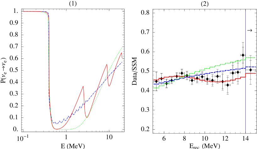
Figure 1: Survival probabilities for $M_{e}\simeq 2.1\cdot 10^{-3}\,\mathrm{eV}$ and $(1/R,m_{e})=(20,0.058)\cdot 10^{-3}\,\mathrm{eV}$ (dotted line), $(1/R,m_{e})=(5,0.035)\cdot 10^{-3}\,\mathrm{eV}$ (solid line), and $(1/R,m_{e})=(0.5,0.012)\cdot 10^{-3}\,\mathrm{eV}$ (dashed line).

Figure 2: Recoil energy spectrum associated with the three survival probabilities in Fig. 2.

The dotted line corresponds to the regime $M_{e}R\ll 1$. The probability does not depend on the precise value of $1/R$ for the energy range shown in Fig. 2 as long as $1/R\gtrsim 7M_{e}$. In this case, in fact, $2E_{\nu}V_{e}^{\text{core}}<M_{e}^{2}+1/R^{2}$, so that the resonant mixing between the electron neutrino and the sterile tower is significant only for the lowest state. The mixing angle with the lowest state $N_{0}$ is $\theta_{0}\simeq m_{e}/M_{e}$. The value of $m_{e}$ corresponds to $\sin^{2}2\theta_{0}\simeq 3\cdot 10^{-3}$ and to a light neutrino mass of $1.7\cdot 10^{-6}\,\mathrm{eV}$. The phenomenology of this case is the same as the one for a model with a single sterile neutrino — the Kaluza Klein origin makes no difference. The SuperKamiokande collaboration has claimed that their data on the day-night asymmetry and especially on the electron recoil energy spectrum disfavour such a scenario involving oscillations into a single sterile neutrino. This is confirmed by Fig. 2, where the dotted line has the highest slope and therefore gives the worse fit of the data, which is well compatible with a flat spectrum.

The presence of additional sterile states reduces the slope of the predicted energy spectrum. This is illustrated by the dashed line in Fig. 2 and the corresponding dashed histogram in Fig. 2. They both correspond to the small $1/R$ case $1/R=0.5\cdot 10^{-3}\,\mathrm{eV}$ in which $M_{e}R>1$. This situation is quite new because a relatively large number of levels undergo resonant conversion. The single resonances are not visible in the figure due to the average over the neutrino production point in the sun. The mass of the light neutrino is now $0.9\cdot 10^{-6}\,\mathrm{eV}$. This case leads to a significant improvement with respect to the single sterile neutrino case with the fit of the total rates (the energy spectrum) at 65% CL (50% CL). Finally, the solid lines in Fig. 2, Fig. 2 represent the intermediate case $1/R=0.005\,\mathrm{eV}$ in which, besides the light state $\hat{\nu}$, three bulk states, $N_{0}$, $N_{1}$ and $N_{2}$, participate in solar oscillations. Fig. 2 shows that the values of the bulk and brane-bulk masses giving the best fit of total rates (within a 25% CL) also beautifully fit the energy spectrum (10% CL). Besides the three examples discussed, the whole range of possible values of $1/R$ also includes the situation in which $M_{e}R\sim 1$ [22], that approximately reproduces the case considered by Dvali and Smirnov [12].

Unlike the energy spectrum, the day-night asymmetry [46, 30] does not discriminate between the different possibilities discussed. In fact, the day-night asymmetry turns out to be small compared to the experimental errors in all cases considered above and therefore is in reasonably good agreement with the present data, given that SK finds only a $1.2\,\sigma$ deviation from zero asymmetry.

For our three sample cases the values of $m_{e}^{2}R/\,\mathrm{eV}$ are of the order of $10^{-7}$ and, hence, compatible with the supernova bounds derived in Section 4.

The scenario discussed leads to various experimental signatures. First of all, a crucial test will be provided by the neutral/charged current ratio measurement in SNO [47]. Moreover, different sterile neutrino scenarios can be distinguished by the shape of the energy spectrum. As discussed, the present data already favours a flatter spectrum, which can be obtained if more than one sterile neutrino takes part in the oscillations. The charged current spectrum that will be measured by SNO could provide additional information. Finally, the measurement of a day-night asymmetry significantly lower than zero would disfavour the scenario with many sterile neutrinos.

5.3 Atmospheric neutrinos

Let us now discuss atmospheric neutrinos. As already pointed out, in a model with small (perturbative) brane-bulk mixing, the small bulk components of the SM neutrinos do not contribute significantly to atmospheric neutrino oscillations. Hence, these oscillations must be due to the three light mass eigenstates. We can, therefore, focus on the first part of eq. (5.8) given by

$$\nu_{i}=\sum_{k=1,2,3}U_{ik}\hat{\nu}_{k}\;.$$ (5.17)

The light masses and the MNS mixing matrix $U$ are determined by the light mass matrix ${m^{\prime}}$ in eq. (5.1). Before constructing an explicit model, let us first discuss some phenomenological requirements on this mass matrix suggested by atmospheric neutrino oscillations. The simplest texture leading to maximal $\nu_{\mu}\leftrightarrow\nu_{\tau}$ mixing is

$${m^{\prime}}=\begin{pmatrix}a&\epsilon_{e\mu}&\epsilon_{e\tau}\\ \epsilon_{e\mu}&\epsilon_{\mu}&1\\ \epsilon_{e\tau}&1&\epsilon_{\tau}\end{pmatrix}\;m_{\mu\tau}\;,$$ (5.18)

where the $\epsilon$ parameters are much smaller than one. The parameter $a$ is not necessarily small but it will be in our explicit model described below.

In the limit in which the $\epsilon$ parameters are vanishing, the muon and tau neutrinos are superpositions of two degenerate states $\hat{\nu}_{2}$ and $\hat{\nu}_{3}$ with mass $|m_{\mu\tau}|$. The small $\epsilon$ parameters (assumed to be real for simplicity) are necessary to generate a mass splitting

$$\Delta m_{23}\simeq\epsilon\,|m_{\mu\tau}|,\qquad\epsilon=\epsilon_{\mu}+\epsilon_{\tau}$$ (5.19)

between the degenerate states and therefore an “atmospheric” squared mass difference ${\Delta m^{2}_{\text{ATM}}}={\Delta m^{2}_{\text{23}}}\simeq 2\epsilon|m_{\mu\tau}|^{2}$. The corresponding mixing angle $\theta_{\mu\tau}$ is almost maximal and it is given by $\sin^{2}2\theta_{\mu\tau}\simeq 1-(\epsilon_{\mu}-\epsilon_{\tau})^{2}/4$. For ${\Delta m^{2}_{\text{12}}}\simeq{\Delta m^{2}_{\text{13}}}\gtrsim{\Delta m^{2}_{\text{ATM}}}$ the parameters $\epsilon_{e\mu}$, $\epsilon_{e\tau}$ are constrained to be small by the $\nu_{e}$ disappearance experiments.

Notice that the simple mechanism described to generate a maximal $\nu_{\mu}\leftrightarrow\nu_{\tau}$ mixing does not work in a three neutrino scenario aiming at explaining at the same time the solar neutrino data. This is because the other two squared mass differences available turn out to be larger than the atmospheric one, unless the parameter $a$ in (5.18) is close to 1 and all neutrino masses are degenerate [40]. If this is not the case and all $\epsilon<1/2$, we have, in fact,

$${\Delta m^{2}_{\text{21}}}\simeq{\Delta m^{2}_{\text{31}}}\gtrsim|m_{\mu\tau}|^{2}>2\epsilon|m_{\mu\tau}|^{2}={\Delta m^{2}_{\text{ATM}}}\;.$$ (5.20)

As a consequence, there is no room for the small ${\Delta m^{2}_{\text{}}}$ required by the solar data. In our case, of course, such a small ${\Delta m^{2}_{\text{}}}$ is not needed since the solar neutrino problem is solved by oscillations into bulk neutrinos.

If the texture (5.18) accounts for atmospheric neutrino oscillations, the two degenerate neutrinos can provide a cosmologically significant source of dark matter. Moreover, the electron neutrino can oscillate into muon or tau neutrinos with a squared mass difference ${\Delta m^{2}_{\text{}}}>{\Delta m^{2}_{\text{ATM}}}$ and small amplitudes $4\epsilon^{2}_{e\mu}$, $4\epsilon^{2}_{e\tau}$ respectively. If the parameter $a$ is small, we have $\Delta m\simeq m_{\mu\tau}$. It is obviously tempting to associate such oscillations with the signal observed by LSND. This then determines the size of $m_{\mu\tau}$ to be $|m_{\mu\tau}|\simeq\sqrt{{\Delta m^{2}_{\text{LSND}}}}$. The MiniBooNE experiment will test this possibility and will cover a relevant portion of the parameter space for such short-baseline oscillations. A short-baseline neutrino factory could further extend the sensitivity in the $\epsilon_{e\mu}$ mixing parameter [48].

Let us now see how the texture (5.18) can be obtained in a model in which the single family discussion of solar neutrino oscillations given above can be embedded. We work in the context of the $\mathbb{Z}_{2}$ invariant models with Majorana bulk mass described in Subsection 5.1.

A simple way to obtain the zeroth order form of eq. (5.18) in which $a$ and the $\epsilon$ parameters vanish is to assume three bulk fermions $\Psi_{e}$, $\Psi_{\mu}$, $\Psi_{\tau}$, a diagonal brane-bulk coupling $m$ and a Majorana mass matrix $M$ with two off-diagonal non vanishing entries. Concretely,

$$\begin{matrix}\phantom{{m}=\,\begin{matrix}\nu_{\tau}\end{matrix}\,\;}\begin{matrix}\Psi_{e}&\Psi_{\mu}&\Psi_{\tau}\end{matrix}\\[2.84526pt] {m}=\,\begin{matrix}\nu_{e}\\ \nu_{\mu}\\ \nu_{\tau}\\ \end{matrix}\,\begin{pmatrix}\makebox[10.38531pt]{$m_{e}$}&\makebox[11.15207pt]{$0$}&\makebox[10.22586pt]{$0$}\\ 0&m_{\mu}&0\\ 0&0&m_{\tau}\end{pmatrix}\end{matrix}\qquad\begin{matrix}\phantom{M=\,\begin{matrix}\Psi_{\tau}\end{matrix}\,\;}\begin{matrix}\Psi_{e}&\makebox[16.61398pt]{$\Psi_{\mu}$}&\makebox[17.54019pt]{$\Psi_{\tau}$}\end{matrix}\\[2.84526pt] M=\,\begin{matrix}\Psi_{e}\\ \Psi_{\mu}\\ \Psi_{\tau}\\ \end{matrix}\,\begin{pmatrix}\makebox[10.38531pt]{$0$}&0&0\\ 0&0&M_{\mu\tau}\\ 0&M_{\mu\tau}&0\end{pmatrix}&{,}\end{matrix}$$ (5.21)

where $M_{\mu\tau}$ can be made real by a phase-redefinition of the bulk fields $\Psi_{\mu}$, $\Psi_{\tau}$. We note that, for a direct application of the results of Subsection 5.1 to this case, we should first diagonalize the matrix $M$ and rewrite the brane-bulk coupling $m$ in the corresponding basis. Alternatively, one can use eq. (3.18) with $m$ and $M$ as in eq. (5.21). Then, we find from eq. (5.1) that the light mass matrix ${m^{\prime}}$ has indeed the structure (5.18) with vanishing parameters $a$, $\epsilon$ and the overall scale $m_{\mu\tau}$ given by

$$m_{\mu\tau}\simeq-\pi Rm_{\mu}m_{\tau}\coth(\pi RM_{\mu\tau})\;.$$ (5.22)

The bulk components of $\nu_{\mu}$ and $\nu_{\tau}$ are small if

$$\pi R|m_{\mu}|^{2}\coth(\pi RM_{\mu\tau})\ll M_{\mu\tau}\quad\text{and}\quad\pi R|m_{\tau}|^{2}\coth(\pi RM_{\mu\tau})\ll M_{\mu\tau}\;,$$ (5.23)

which implies that

$$|m_{\mu\tau}|\ll M_{\mu\tau}\;.$$ (5.24)

The form (5.21) of the brane-bulk mixing and of the Majorana mass matrix can be enforced by means of symmetries acting both on brane and bulk fields. For example, let us introduce three individual lepton numbers $L_{e,\mu,\tau}$ for each generation with the bulk fermions $\Psi_{e,\mu,\tau}$ carrying the same charge as the corresponding neutrinos on the brane. Let us further require that $L_{\mu}-L_{\tau}$ and $L_{e}$ are both conserved. This leads exactly to the structure given in eq. (5.21). In order to generate the small $\epsilon$ corrections to the texture (5.18) one has to break these symmetries. This can be done by small off-diagonal brane-bulk couplings or small Majorana masses replacing the zero entries in the matrices (5.21).

To see this in more detail, let us first discuss how solar neutrino oscillations along the lines of Section 5.2 can be embedded into the model. As a consequence of eqs. (5.21), the electron neutrino only mixes with the bulk field $\Psi_{e}$. The solar neutrino phenomenology described in Section 5.2 follows once $L_{e}$ is broken by a non-vanishing Majorana mass $M_{e}$. The smallness of $M_{e}\sim(2\,\text{--}\,3)\cdot 10^{-3}\,\mathrm{eV}$ compared to $M_{\mu\tau}\gg|m_{\mu\tau}|>\sqrt{{\Delta m^{2}_{\text{ATM}}}}$ is then a consequence of the approximate conservation of $L_{e}$. Analogously, a small breaking of $L_{\mu}-L_{\tau}$ can produce the small diagonal entries $\epsilon_{\mu}$ and $\epsilon_{\tau}$ necessary to generate the atmospheric ${\Delta m^{2}_{\text{}}}$. This can be accomplished by switching on the $L_{\mu}-L_{\tau}$ breaking and $L_{e}$ conserving entries in the bulk Majorana matrix or in the brane-bulk mixing matrix. Once $L_{e}$ and $L_{\mu}-L_{\tau}$ are both broken, the $\nu_{e}$-$\nu_{\mu}$ mixing in (5.18) can be easily generated in the same way. In general, $L_{\mu}-L_{\tau}$ can be broken both by bulk Majorana mass terms and by brane-bulk couplings. The most general case, corresponding to replacing all zero entries in the texture (5.21) by small corrections, leads to a quite complicated mass matrix for the light neutrinos. As an illustration, let us consider a somewhat simplified case where we break $L_{\mu}-L_{\tau}$ by brane-bulk terms only. That is, instead of eq. (5.21) we now consider matrices

$$m=\left(\begin{array}[]{ccc}m_{e}&\delta m_{e\mu}&\delta m_{e\tau}\\ \delta m_{\mu e}&m_{\mu}&\delta m_{\mu\tau}\\ \delta m_{\tau e}&\delta m_{\tau\mu}&m_{\tau}\end{array}\right)\qquad M=\left(\begin{array}[]{ccc}M_{e}&0&0\\ 0&0&M_{\mu\tau}\\ 0&M_{\mu\tau}&0\end{array}\right)$$ (5.25)

where $\delta m_{e\mu}$, $\delta m_{e\tau}$ and $\delta m_{\mu\tau}$ are small corrections. Expanding to first order in these corrections and using the parameterization (5.18), we find for the $\epsilon$ perturbations to the mass matrix

$$\epsilon_{\mu} = \frac{2\delta m_{\tau\mu}}{m_{\tau}}$$ (5.26)

$$\epsilon_{\tau} = \frac{2\delta m_{\mu\tau}}{m_{\mu}}$$ (5.27)

$$\epsilon_{e\mu} = \frac{m_{e}\coth(\pi RM_{e})\delta m_{e\mu}+m_{\mu}\coth(\pi RM_{\mu\tau})\delta m_{\tau e}}{m_{\mu}m_{\tau}\coth(\pi RM_{\mu\tau})}$$ (5.28)

$$\epsilon_{e\tau} = \frac{m_{e}\coth(\pi RM_{e})\delta m_{e\tau}+m_{\tau}\coth(\pi RM_{\mu\tau})\delta m_{\mu e}}{m_{\mu}m_{\tau}\coth(\pi RM_{\mu\tau})}\;.$$ (5.29)

The atmospheric square mass difference is then related to the corrections by

$$\epsilon=\frac{\Delta m_{\rm ATM}^{2}}{2|m_{\mu\tau}|^{2}}=2\left(\frac{\delta m_{\mu\tau}}{m_{\mu}}+\frac{\delta m_{\tau\mu}}{m_{\tau}}\right)\;.$$ (5.30)

The amount of $L_{\mu}-L_{\tau}$ breaking needed for a correct account of atmospheric neutrino oscillations is, therefore, variable since it depends on $m_{\mu\tau}$ which is not fixed by solar or atmospheric data. If, in addition, we require an explanation of the LSND signal we have $m_{\mu\tau}\simeq\sqrt{{\Delta m^{2}_{\text{LSND}}}}$ resulting in a $L_{\mu}-L_{\tau}$ breaking $\epsilon$ of the order $\sqrt{{\Delta m^{2}_{\text{ATM}}}/{\Delta m^{2}_{\text{LSND}}}}$. For a hierarchical structure of the brane-bulk mass matrix, that is $m_{e}\ll m_{\mu}\ll m_{\tau}$ and $\delta m_{\tau e}\lesssim\delta m_{\mu e}$, the $e$–$\mu$ mixing angle $\theta_{e\mu}$ is given by

$$\theta_{e\mu}=\frac{\epsilon_{e\mu}+\epsilon_{e\tau}}{\sqrt{2}}\simeq\frac{\delta m_{\mu e}}{\sqrt{2}m_{\mu}}\;.$$ (5.31)

This angle should then be in the LSND range which can be easily accommodated by choosing $\delta m_{e\mu}$. Notice that such a small $\nu_{e}$-$\nu_{\mu}$ mixing can also generate a small mixing between the electron neutrino and the towers of sterile neutrinos associated with $\Psi_{\mu,\tau}$, heavier than the one we have used to deplete the solar neutrino flux. Due to the large mass splitting between the lightest electron neutrino and the lowest mode of the heavy towers, such a small mixing can not be MSW-enhanced and consequently does not affect the solar neutrino phenomenology. However, it may give rise to a non-negligible contribution to the light electron neutrino mass.

It is clear, that a parallel discussion can be carried out for $L_{\mu}-L_{\tau}$ breaking induced by bulk Majorana mass terms. However, the above example is sufficient to show that all oscillation data can be explained in terms of our model. We, therefore, will not carry this out explicitly.

We have already mentioned that parameters in the model associated with the first generation are compatible with the supernova bound. However, we also have to worry about the supernova bound due to resonant conversion of $\nu_{\mu}$ and $\nu_{\tau}$ into their respective Kaluza-Klein states. As the above equations show, the particle phenomenology of the model is not very sensitive to $M_{\mu\tau}$ as long as this mass is larger than $m_{\mu\tau}$ and smaller than the fundamental scale. Therefore, we can choose $M_{\mu\tau}$ larger than $\sqrt{2EV}$ where $V$ is the matter potential in the core of the supernova and $E$ is the neutrino energy. This avoids any problem with the supernova bound due to conversion of $\nu_{\mu}$ and $\nu_{\tau}$ into their associated bulk states. As discussed, the large value of $M_{\mu\tau}$ (as compared to $M_{e}$) can be attributed to the approximate conservation of $L_{e}$.

To summarize, in the framework of a $\mathbb{Z}_{2}$-symmetric theory we have accommodated solar neutrino oscillations, naturally maximal $\nu_{\mu}\leftrightarrow\nu_{\tau}$ oscillations, two degenerate neutrinos providing a cosmologically significant source of dark matter and $\nu_{e}\leftrightarrow\nu_{\mu}$ oscillations with a ${\Delta m^{2}_{\text{}}}$ larger than the atmospheric one, that can be used to accommodate the LSND signal. The spectrum of parameters in the bulk Majorana mass matrix and the brane-bulk mixing matrix (5.25) we need is the following.

• The value of $1/R$ should be compatible with its lower experimental limit emerging from Cavendish-type experiments.

• To get the best agreement with the SuperKamiokande energy spectrum, $1/R$ should be less that $10^{-2}\,\mathrm{eV}$, in such a way that more than a sterile state is involved.

• To explain the solar neutrino deficit $L_{e}$ has to be broken by an electron bulk Majorana mass $M_{e}\sim(2\,\text{--}\,3)\cdot 10^{-3}\,\mathrm{eV}$. Furthermore, we need the electron brane-bulk coupling to be of the order $m_{e}=\mathcal{O}\left(10^{-(4\,\text{--}\,5)}\,\mathrm{eV}\right)$.

• If the LSND signal has to be explained the parameter $|m_{\mu\tau}|$ as given in eq. (5.22) should have the value $|m_{\mu\tau}|=\sqrt{{\Delta m^{2}_{\text{LSND}}}}=\mathcal{O}\left(1\,\mathrm{eV}\right)$. This requires that the quantity $\sqrt{m_{\mu}m_{\tau}}$ is close to the geometric average of $\sqrt{{\Delta m^{2}_{\text{LSND}}}}$ and the smallest between $M_{\mu\tau}$ and $R^{-1}$.

• We need $M_{\mu\tau}\gg|m_{\mu\tau}|$, in order to have a small bulk component in $\nu_{\mu}$ and $\nu_{\tau}$ and a quasi-unitary light mixing matrix $U$. A value of $M_{\mu\tau}$ larger than $\sqrt{2EV}$ avoids any potential problems with the conversion of $\nu_{\mu}$ and $\nu_{\tau}$ into their associated bulk states in the supernova. Also the hierarchy between $m_{\mu}$ and $m_{\tau}$ must be smaller than the hierarchy between $|m_{\mu\tau}|$ and $M_{\mu\tau}$.

• To explain the atmospheric squared mass difference we need to break $L_{\mu}-L_{\tau}$. If this is done be brane-bulk mixing and we use the LSND result the level of this breaking is specified by the condition $\delta m_{\mu\tau}/m_{\mu}\simeq\Delta m_{\rm ATM}^{2}/\Delta m_{\rm LSND}^{2}$.

• In order to get the $e$–$\mu$ mixing required by LSND we need to consider terms breaking $L_{e}$ and $L_{\mu}-L_{\tau}$. If this is achieved by perturbing the brane-bulk mixing the level of this breaking is determined by $\theta_{e\mu}=\delta m_{\mu e}/m_{\mu}$. A smaller value of $\theta_{e\mu}$ than needed to account for the LSND signal could be within the reach of MiniBooNE or a short-baseline neutrino factory.

Finally, let us mention that there are alternative models within the general class considered in this paper which provide similar possibilities to explain the various oscillation phenomena. For example, in the context of the models with $U(1)$ lepton number symmetry and Dirac bulk masses which we have briefly discussed, an analogous (and complementary) scheme using the brane-bulk mixings $m^{c}$ as a source of $U(1)$-breaking and light neutrino masses can be constructed [22]. Then, the overall $U(1)$ can be considered as a subgroup of the individual lepton number groups and the model with $L_{\mu}-L_{\tau}$ and $L_{e}$ symmetry arises at an intermediate stage in the necessary breaking of these individual lepton numbers.

6 Conclusion

In this paper, we have systematically studied five-dimensional brane-world models of neutrino physics based on flat compactifications. Motivated by the expectation from string theory, we have particularly focused on the effect of bulk mass terms for the sterile neutrinos. For such models we have presented a number of general results. We have pointed out that there are four different types of bulk mass terms, namely scalar Dirac and Majorana masses as well as vector-like Dirac and Majorana masses. While the scalar masses can be thought of as being generated by the VEV of a bulk scalar field and respect five-dimensional Lorentz invariance the vector masses are due to the VEV of the fifth component of a bulk vector field and break five-dimensional Lorentz invariance. We have analyzed the (unperturbed) spectrum of bulk Kaluza-Klein states in the presence of these mass terms and have found a crucial difference between scalar and vector-like masses. Whereas scalar masses constitute a lower bound on the spectrum this is not the case for vector-like masses. For arbitrary values of these masses (and in the absence of scalar masses) there will always be states with masses of order $1/R$. In the presence of small brane-bulk couplings, we have presented perturbative results based on a see-saw type approximation. In particular, we have shown in general that, in this approximation, the electroweak eigenstates are mainly given by a superposition of three light mass eigenstates with small admixtures of massive Kaluza-Klein modes. We have also shown that the relevant parameters associated with these two sectors can be controlled quite independently by choosing the various mass terms in the action appropriately. This opens up the possibility of associating some of the observed oscillation phenomena with “standard oscillations” into the light states and some others with oscillations into heavy bulk states. To complement the perturbative approach, we have also presented a general formalism and results for the exact diagonalization of the mass matrix.

These general results have been applied to construct a specific brane-world model compatible with all presently observed oscillation phenomena. The model is based on a $\mathbb{Z}_{2}$ orbifolding and broken $L_{e}$ and $L_{\mu}-L_{\tau}$ symmetries. The solar neutrino deficit is explained by small mixing angle oscillations into the tower of heavy bulk states. It has been shown that this, contrary to the case of small mixing angle oscillations into a single sterile neutrino, is compatible with recent SuperKamiokande results. The model also naturally leads to a maximal $\nu_{\mu}\leftrightarrow\nu_{\tau}$ mixing that accounts for the atmospheric neutrino result. In addition, it allows to accommodate the LSND observation and may lead to a significant neutrino dark matter component.

We have also analyzed constraints from supernova energy loss on such brane-world models and have demonstrated that our specific model is consistent with these constraints.

In summary, we have shown that the inclusion of bulk mass terms leads to a rich structure of brane-world models for neutrino masses which can be used to construct models compatible with all known experimental results.

Appendix A Spinor conventions in four and five dimensions

In this Appendix, we collect the properties of five-dimensional gammma matrices and spinors which we are using in the main part of the paper.

The five-dimensional gamma matrices $\gamma_{\alpha}$, where $\alpha,\beta,\cdots=0,1,2,3,4$, satisfy the Clifford algebra

$$\{\gamma_{\alpha},\gamma_{\beta}\}=2\eta_{\alpha\beta}=2\,\text{diag}(1,-1,-1,-1,-1)\;.$$ (A.1)

Note, that we are using the “mostly minus” Minkowski metric throughout. As usual, the generators $\Sigma_{\alpha\beta}$ of the Lorentz group $SO(4,1)$ can be obtained by

$$\Sigma_{\alpha\beta}=\frac{i}{4}[\gamma_{\alpha},\gamma_{\beta}]\;.$$ (A.2)

The hermitian conjugate of the gamma matrices is generated by $\gamma_{0}$ according to

$$(\gamma_{\alpha})^{\dagger}=\gamma_{0}\gamma_{\alpha}\gamma_{0}\;.$$ (A.3)

Similarly, to express the complex conjugate and the transpose of the gamma matrices we introduce a matrix $B$ and a charge conjugation matrix $C$. Their defining properties are

$$(\gamma_{\alpha})^{*} = B\gamma_{\alpha}B^{-1}$$ (A.4)

$$(\gamma_{\alpha})^{T} = C\gamma_{\alpha}C^{-1}\;.$$ (A.5)

Obviously, this implies that $C=B^{T}\gamma_{0}$. We note, that the matrices $B$ and $C$ square to $-1$ unlike their four-dimensional counterparts which square to one.

A five-dimensional Dirac spinor $\Psi$ has four complex components. Under infinitesimal Lorentz transformations it transforms as

$$\delta\Psi=\frac{i}{2}\omega_{\alpha\beta}\Sigma_{\alpha\beta}\Psi\;.$$ (A.6)

We define the conjugated spinor $\bar{\Psi}$ and the charge conjugated spinor $\Psi^{c}$ by

$$\bar{\Psi}=\Psi^{\dagger}\gamma_{0}\;,\qquad\Psi^{c}=B^{-1}\Psi^{*}=C\bar{\Psi}^{T}\;.$$ (A.7)

Note that, under infinitesimal Lorentz transformations, $\Psi^{c}$ transforms in the same way as $\Psi$. Furthermore, we note that $(\Psi^{c})^{c}=-\Psi$. The minus sign in this relation is due to the above mentioned fact that $B^{2}=C^{2}=-1$ and precludes the existence of five-dimensional Majorana spinors.

For our purpose of dimensional reduction to four dimensions, we need to make contact between the above five-dimensional spinors and Weyl spinors. To do this, it is useful to introduce explicit representations for the gamma matrices. We choose

$$\gamma_{\mu}=\begin{pmatrix}0&\sigma_{\mu}\\ \bar{\sigma}_{\mu}&0\end{pmatrix}\;,\qquad\gamma_{4}=\gamma_{0}\gamma_{1}\gamma_{2}\gamma_{3}=\begin{pmatrix}-i\mathbf{1}_{2}&0\\ 0&i\mathbf{1}_{2}\end{pmatrix}\;$$ (A.8)

where $\sigma_{\mu}=(\mathbf{1}_{2},-\sigma_{i})$, $\bar{\sigma}_{\mu}=(\mathbf{1}_{2},\sigma_{i})$ and $\sigma_{i}$ are the Pauli matrices. Furthermore, we have the matrix $\gamma_{5}$ defined as usual by

$$\gamma_{5}=i\gamma_{4}=\begin{pmatrix}\mathbf{1}_{2}&0\\ 0&-\mathbf{1}_{2}\end{pmatrix}$$ (A.9)

and satisfying $(\gamma_{5})^{2}=1$. For the matrices $B$ and $C$ we can choose, in this representation

$$B=\gamma_{2}\gamma_{4}=-\begin{pmatrix}0&\epsilon\\ \epsilon&0\end{pmatrix}\;,\qquad C=\gamma_{2}\gamma_{0}\gamma_{4}=\begin{pmatrix}\epsilon&0\\ 0&\epsilon\end{pmatrix}$$ (A.10)

where $\epsilon=i\sigma_{2}$ is the two-dimensional epsilon symbol.

A five-dimensional Dirac spinor $\Psi$ is decomposed into two left-handed Weyl spinors $\xi$ and $\eta$ as

$$\Psi=\begin{pmatrix}\bar{\xi}\\ \eta\end{pmatrix}\;.$$ (A.11)

The conjugated spinor $\xi$ is defined by $\bar{\xi}=\epsilon\xi^{*}$. Using the above explicit representation, it is easy to obtain the relations

$$\bar{\Psi}=\begin{pmatrix}\eta^{\dagger}&-\xi^{T}\epsilon\end{pmatrix}\;,\qquad\Psi^{c}=\begin{pmatrix}\bar{\eta}\\ -\xi\end{pmatrix}\;,\qquad\bar{\Psi}^{c}=\begin{pmatrix}-\xi^{\dagger}&-\eta^{T}\epsilon\end{pmatrix}$$ (A.12)

which will be useful for the dimensional reduction to four dimensions. To write our four-dimensional effective action in a compact form we furthermore adopt the following notation for Weyl mass terms

$$\xi_{1}\xi_{2}\equiv\xi_{1}^{T}\epsilon\xi_{2}\;.$$ (A.13)

where $\xi_{1}$ and $\xi_{2}$ are two (left-handed) Weyl spinors.

Appendix B Exact diagonalization

We first consider the general case of three standard model neutrinos $\mathbf{\nu}=(\nu_{e},\nu_{\mu},\nu_{\tau})^{T}$ and $\kappa$ “bulk” neutrinos $\mathbf{\chi}=(\chi_{1}\ldots\chi_{\kappa})^{T}$. The associated Majorana mass matrix is of the general form

$$\begin{matrix}\phantom{{\cal M}=\,\begin{matrix}\eta_{n}\end{matrix}\,\;}\begin{matrix}\mathbf{\nu}^{T}&\mathbf{\chi}^{T}\end{matrix}\\[2.84526pt] {\cal M}=\,\begin{matrix}\mathbf{\nu}\\ \mathbf{\chi}\\ \end{matrix}\,\begin{pmatrix}\makebox[8.9901pt]{$0$}&\makebox[10.30719pt]{$\mathbf{v}^{T}$}\\ \mathbf{v}&\mathbf{D}\end{pmatrix}&{,}\end{matrix}$$ (B.1)

where $\mathbf{v}$ is a $\kappa\times 3$ matrix and $\mathbf{D}$ is a $\kappa\times\kappa$ symmetric matrix. When the set of $\mathbf{\chi}$ fields is allowed do be infinite, the results can be applied to the diagonalization of the mass matrix (2.50), originating from the five-dimensional brane-world theory, by making the obvious identifications

$$\mathbf{\nu}=(\nu_{e},\nu_{\mu},\nu_{\tau})^{T}\qquad\mathbf{\chi}={(\xi_{n},\eta_{n})_{n\in\mathbb{Z}}}^{T}$$ (B.2a)

$$\mathbf{v}^{T}=(m^{T},{m^{c}}^{T})_{n\in\mathbb{Z}}\qquad\mathbf{D}=({\cal M}_{n}\delta_{-m,n})_{n,m\in\mathbb{Z}}.$$ (B.2b)

While, in this paper, we focus on cases where $\mathbf{D}$ has such a block structure, the general formulae below also apply to more complicated cases. A more complicated $\mathbf{D}$ is generated if the bulk mass terms effectively depend on the coordinates of the additional dimension. Such an explicit coordinate dependence may arise in orbifold models or due to a non-flat vacuum solution.

Since, with the usual approximations, the equations for neutrino propagation only involve ${\cal M}^{\dagger}{\cal M}$, we actually diagonalize the matrix

$${\cal M}^{2}_{\text{eff}}={\cal M}^{\dagger}{\cal M}+\begin{pmatrix}A&0\\ 0&0\end{pmatrix}=\begin{pmatrix}\mathbf{v}^{\dagger}\mathbf{v}+A&\mathbf{v}^{\dagger}\mathbf{D}\\ \bar{\mathbf{D}}\mathbf{v}&\bar{\mathbf{D}}\mathbf{D}+\bar{\mathbf{v}}\mathbf{v}^{T}\end{pmatrix}\;,$$ (B.3)

where the hermitian matrix $A=\sqrt{2}E_{\nu}V$ takes matter effects into account. As usual, $E_{\nu}$ represents the neutrino energy and $V$ the matter induced potential. The eigenvalue equations for the generic mass eigenstate

$$\hat{\nu}=\mathbf{\alpha}^{\dagger}\mathbf{\nu}+\mathbf{\beta}^{\dagger}\mathbf{\chi}$$ (B.4)

(in obvious matrix notations) are

$$\left\{\begin{aligned} \mbox{}&(\mathbf{v}^{\dagger}\mathbf{v}+A)\mathbf{\alpha}+\mathbf{v}^{\dagger}\mathbf{D}\mathbf{\beta}=\lambda^{2}\alpha\\ \mbox{}&\bar{\mathbf{D}}\mathbf{v}\mathbf{\alpha}+\bar{\mathbf{D}}\mathbf{D}\mathbf{\beta}+\bar{\mathbf{v}}\mathbf{v}^{T}\mathbf{\beta}=\lambda^{2}\mathbf{\beta}\end{aligned}\;,\right.$$ (B.5)

where $\lambda^{2}$ is the corresponding real (possibly negative) eigenvalue.

As shown in Appendix B.2 and further explained in the main text, it often happens that some of the eigenvectors of the matrix $\bar{\mathbf{D}}\mathbf{D}$ are also eigenvectors of the matrix ${\cal M}$ and as such decouple from the light neutrinos $\mathbf{\nu}$. The vector space generated by such “unperturbed” mass eigenstates coincides with the maximal space of vectors in the form eq. (B.4) such that $\mathbf{\alpha}=0$, $\mathbf{\beta}$ is orthogonal to both $\bar{\mathbf{v}}$ and $\bar{\mathbf{D}}\mathbf{v}$ and the space is invariant under $\bar{\mathbf{D}}\mathbf{D}$. In other words the unperturbed eigenstates are in the form $\hat{\nu}_{\rm unp}=\mathbf{\beta}^{\dagger}\mathbf{\chi}$, with $\mathbf{\beta}$ solving the following set of equations

$$\left\{\begin{aligned} \mbox{}&\bar{\mathbf{D}}\mathbf{D}\mathbf{\beta}=\lambda^{2}\mathbf{\beta}\\ \mbox{}&\mathbf{v}^{\dagger}\mathbf{D}\mathbf{\beta}=0\\ \mbox{}&\mathbf{v}^{T}\mathbf{\beta}=0\end{aligned}\right.\;.$$ (B.6)

Let us now derive the eigenvalue equations for the “perturbed” eigenstates. In this case, it is reasonable to assume that $\lambda^{2}$ is not an eigenvalue of $\bar{\mathbf{D}}\mathbf{D}$, so that $\lambda^{2}-\bar{\mathbf{D}}\mathbf{D}$ can be inverted . Then, using eqs. (B.5) $\mathbf{v}^{\dagger}\mathbf{D}\mathbf{\beta}$ and $\mathbf{\beta}$ can be expressed in terms of $\tilde{\mathbf{\alpha}}\equiv\mathbf{v}^{T}\mathbf{\beta}$ and $\mathbf{\alpha}$. In particular,

$$\mathbf{\beta}=\frac{1}{\lambda^{2}-\bar{\mathbf{D}}\mathbf{D}}\left[\bar{\mathbf{D}}\mathbf{v}\mathbf{\alpha}+\bar{\mathbf{v}}(\tilde{\mathbf{\alpha}})\right]\;.$$ (B.7)

By taking appropriate projections, one then gets the following equations for $\tilde{\mathbf{\alpha}}=\mathbf{v}^{T}\mathbf{\beta}$ and $\mathbf{\alpha}=(\lambda^{2}-\mathbf{v}^{\dagger}\mathbf{v}-A)^{-1}\mathbf{v}^{\dagger}\mathbf{D}\mathbf{\beta}$:

$$\left\{\begin{aligned} \mbox{}&\left(\mathbf{1}-\mathbf{v}^{T}\frac{1}{\lambda^{2}-\bar{\mathbf{D}}\mathbf{D}}\bar{\mathbf{v}}\right)\tilde{\mathbf{\alpha}}=\mathbf{v}^{T}\frac{1}{\lambda^{2}-\bar{\mathbf{D}}\mathbf{D}}\bar{\mathbf{D}}\mathbf{v}\mathbf{\alpha}\\ \mbox{}&\left(\lambda^{2}-\mathbf{v}^{\dagger}\mathbf{v}-A-\mathbf{v}^{\dagger}\mathbf{D}\frac{1}{\lambda^{2}-\bar{\mathbf{D}}\mathbf{D}}\bar{\mathbf{D}}\mathbf{v}\right)\mathbf{\alpha}=\mathbf{v}^{\dagger}\mathbf{D}\frac{1}{\lambda^{2}-\bar{\mathbf{D}}\mathbf{D}}\bar{\mathbf{v}}\tilde{\mathbf{\alpha}}\end{aligned}\right.\;.$$ (B.8)

Eqs. (B.8) can have two different sets of solutions. In some cases there can be “decoupled solutions” corresponding to eigenstates decoupled from the SM eigenstates, that is $\mathbf{\alpha}=0$. The decoupled states of squared mass $\lambda^{2}$ are therefore in the form

$$\hat{\nu}_{\text{dec}}=\tilde{\mathbf{\alpha}}^{\dagger}\mathbf{v}^{T}\frac{1}{\lambda^{2}-\bar{\mathbf{D}}\mathbf{D}}\mathbf{\chi}\;,$$ (B.9)

where $\tilde{\mathbf{\alpha}}=\mathbf{v}^{T}\mathbf{\beta}$ must satisfy

$$\left\{\begin{aligned} \mbox{}&\left(\mathbf{1}-\mathbf{v}^{T}\frac{1}{\lambda^{2}-\bar{\mathbf{D}}\mathbf{D}}\bar{\mathbf{v}}\right)\tilde{\mathbf{\alpha}}=0\\ \mbox{}&\mathbf{v}^{\dagger}\mathbf{D}\frac{1}{\lambda^{2}-\bar{\mathbf{D}}\mathbf{D}}\bar{\mathbf{v}}\tilde{\mathbf{\alpha}}=0\end{aligned}\right.\;.$$ (B.10)

Although such decoupled (but not unperturbed) eigenstates are not always present, we will see in Appendix B.1 an example in which they are relevant. Also note that the equations for both the unperturbed and the decoupled states do not depend on matter effects encoded in $A$. Therefore, these states are insensitive to matter effects as one would intuitively expect.

The generic solutions of eqs. (B.8) correspond to states which couple to the SM eigenstates $\mathbf{\nu}$ and, therefore, have $\mathbf{\alpha}\neq 0$. In this case, if follows from eqs. (B.8) that $\lambda^{2}$ is an eigenvalue if the following equation has a non-trivial solution for $\mathbf{\alpha}$:

$$\left[\lambda^{2}\left(\mathbf{1}-\mathbf{v}^{\dagger}\frac{1}{\lambda^{2}-\mathbf{D}\bar{\mathbf{D}}}\mathbf{v}\right)-A\right]\mathbf{\alpha}\\ =\mathbf{v}^{\dagger}\mathbf{D}\frac{1}{\lambda^{2}-\bar{\mathbf{D}}\mathbf{D}}\bar{\mathbf{v}}\left(\mathbf{1}-\mathbf{v}^{T}\frac{1}{\lambda^{2}-\bar{\mathbf{D}}\mathbf{D}}\bar{\mathbf{v}}\right)^{-1}\mathbf{v}^{T}\frac{1}{\lambda^{2}-\bar{\mathbf{D}}\mathbf{D}}\bar{\mathbf{D}}\mathbf{v}\mathbf{\alpha}\;.$$ (B.11)

In the case of a single family and no matter effects this eigenvalue equation becomes

$$\lambda^{2}\left|1-\mathbf{v}^{T}\frac{1}{\lambda^{2}-\bar{\mathbf{D}}\mathbf{D}}\bar{\mathbf{v}}\right|^{2}=\left|\mathbf{v}^{\dagger}\mathbf{D}\frac{1}{\lambda^{2}-\bar{\mathbf{D}}\mathbf{D}}\bar{\mathbf{v}}\right|^{2}\;.$$ (B.12)

The eigenspace corresponding to the eigenvalue $\lambda^{2}$ is parameterized by the values of $\mathbf{\alpha}$ solving the above equation. By using eq. (B.7) with $\tilde{\mathbf{\alpha}}$ obtained from the first of eqs. (B.8) we find the following mass eigenstate associated with $\lambda^{2}$ and $\mathbf{\alpha}$.

$$\hat{\nu}=\mathbf{\alpha}^{\dagger}\left[\nu+\mathbf{v}^{\dagger}\mathbf{D}\left[\mathbf{1}+\frac{1}{\lambda^{2}-\bar{\mathbf{D}}\mathbf{D}}\bar{\mathbf{v}}\left(\mathbf{1}-\mathbf{v}^{T}\frac{1}{\lambda^{2}-\bar{\mathbf{D}}\mathbf{D}}\bar{\mathbf{v}}\right)^{-1}\mathbf{v}^{T}\right]\frac{1}{\lambda^{2}-\bar{\mathbf{D}}\mathbf{D}}\chi\right]\;.$$ (B.13)

We now specialize these results to the case of a mass matrix $\mathbf{D}$ with block structure as in eqs. (B.1), a single SM family $\nu$ and a single bulk fermion $(\xi_{n},\eta_{n})_{n\in\mathbb{Z}}$. This is done for two cases, namely for a Dirac and a Majorana bulk mass term.

B.1 Dirac bulk masses

We first consider the simple case with vanishing Majorana-type terms, that is $M_{S}=M_{V}=0$ and $m^{c}=0$, and a Dirac bulk mass term with a scalar components only, that is $\mu\equiv\mu_{S}$, $\mu_{V}=0$. Such a pattern is realized in the context of a model with $U(1)$ lepton number symmetry. Furthermore, we also include matter effects.

The unperturbed eigenstates can be derived from eqs. (B.6). For each $n\geq 1$ there are two unperturbed eigenstates with mass $\sqrt{\mu^{2}+n^{2}/R^{2}}$, namely

$$\frac{\xi_{n}-\xi_{-n}}{\sqrt{2}}\qquad\text{and}\qquad\frac{e^{-i\phi_{n}}\eta_{n}-e^{i\phi_{n}}\eta_{-n}}{\sqrt{2}}\;.$$ (B.14)

Here, the phase $\phi_{n}$ is defined by $\mu+in/R=e^{i\phi_{n}}\sqrt{\mu^{2}+n^{2}/R^{2}}$.

In this model decoupled eigenstates are present as well. In fact, as a consequence of the U(1) symmetry, the second equation in (B.10) is automatically satisfied. This is a very particular property of the $U(1)$ symmetric model and will generically not be the case for other model. The first equation in (B.10) then leads to the eigenvalue equation

$$\pi R|m|^{2}\cot\pi R\sqrt{\lambda^{2}-\mu^{2}}=\sqrt{\lambda^{2}-\mu^{2}}\;.$$ (B.15)

For each $\lambda$ solving this equation one obtains a decoupled state of the form

$$\hat{\nu}_{\text{dec}}=\frac{1}{\sqrt{N}}\sum_{n\in\mathbb{Z}}\frac{m\lambda}{\lambda^{2}-\mu^{2}-n^{2}/R^{2}}\,\xi_{n}\;,$$ (B.16)

The normalization factor $N$ in eq. (B.16) is given by

$$2N=\frac{\lambda^{2}}{|m|^{2}}+\frac{\lambda^{2}}{\lambda^{2}-\mu^{2}}\left(1+\pi^{2}R^{2}|m|^{2}\right)\;.$$ (B.17)

The equation for the masses $\lambda$ of the coupled eigenstates is given by

$$\lambda^{2}\frac{\pi R|m|^{2}}{\sqrt{\lambda^{2}-\mu^{2}}}\cot\pi R\sqrt{\lambda^{2}-\mu^{2}}+A=\lambda^{2}\;.$$ (B.18)

This eigenvalue equation has a single solution with $\lambda^{2}<\mu^{2}$, as can be seen by using the relation $\cot(\sqrt{-x})/\sqrt{-x}=-\coth(\sqrt{x})/\sqrt{x}$. In vacuum, we have $\lambda^{2}=0$, as a consequence of the U(1) symmetry. The associated state with mass $\lambda^{2}$ reads

$$\hat{\nu}=\frac{1}{\sqrt{N}}\left[\nu+\sum_{n\in\mathbb{Z}}\frac{\bar{m}(\mu-in/R)}{\lambda^{2}-\mu^{2}-n^{2}/R^{2}}\,\eta_{n}\right]\;.$$ (B.19)

The normalization factor $N$ in eq. (B.19) is given by 

$$2N=\frac{(\lambda^{2}-A)^{2}+2A|m|^{2}}{\lambda^{2}|m|^{2}}+\frac{\lambda^{2}(1+\pi^{2}R^{2}|m|^{2})-A}{\lambda^{2}-\mu^{2}}\;.$$ (B.20)

In vacuum, the masses of the coupled eigenvalues coincide with the masses of the decoupled ones, with the exception of $\lambda=0$ which is only a coupled eigenvalue. Also, the normalization factors in eqs. (B.16) and (B.19) coincide in vacuum. Coupled and non-coupled states can be combined to form left and right-handed components of Dirac fermions.

B.2 Majorana bulk masses

We now consider the case of a vanishing Dirac mass, $\mu=0$ and furthermore assume that $m^{c}=0$ and $M_{V}=0$. We keep the scalar Majorana mass $M\equiv M_{S}$. This theory is invariant under the $\mathbb{Z}_{2}$ symmetry.

The unperturbed eigenstates can be derived from eqs. (B.6). For each $n\geq 1$ there are two unperturbed eigenstates with mass $\sqrt{M^{2}+n^{2}/R^{2}}$ corresponding to the $\mathbb{Z}_{2}$-odd combinations

$$\frac{\xi_{n}-\xi_{-n}}{\sqrt{2}}\qquad\text{and}\qquad\frac{\eta_{n}+\eta_{-n}}{\sqrt{2}}\;$$ (B.21)

$\eta_{0}$ is the unperturbed eigenstate corresponding to $n=0$. There are no decoupled eigenstates.

The exact masses $\lambda$ of the coupled states are determined by eq. (B.11), which in our case becomes

$$\left[\lambda^{2}(1-x)-A\right](1-x)=M^{2}x^{2}\;,$$ (B.22)

where

$$x=\pi R|m|^{2}\frac{\cot\pi R\sqrt{\lambda^{2}-M^{2}}}{\sqrt{\lambda^{2}-M^{2}}}\;.$$ (B.23)

By solving for $x$, Eq. (B.22) can be written as

$$\pi R|m|^{2}\frac{\cot\pi R\sqrt{\lambda^{2}-M^{2}}}{\sqrt{\lambda^{2}-M^{2}}}=\frac{\lambda}{\lambda\pm M}\;.$$ (B.24)

The corresponding mass eigenstates are

$$\hat{\nu}=\frac{1}{\sqrt{N}}\left[\nu+\sum_{n\in\mathbb{Z}}\frac{\bar{m}}{\lambda^{2}-M^{2}-n^{2}/R^{2}}\left(i\frac{n}{R}\eta_{n}+\frac{M}{1-x}\xi_{n}\right)\right]\;,$$ (B.25)

where $N$ is a normalization factor.

References

- [1] P. Horava and E. Witten, “Eleven-Dimensional Supergravity on a Manifold with Boundary”, Nucl. Phys. B475 (1996) 94, hep-th/9603142.
- [2] E. Witten, “Strong Coupling Expansion Of Calabi-Yau Compactification”, Nucl. Phys. B471 (1996) 135, hep-th/9602070.
- [3] P. Horava, “Gluino condensation in strongly coupled heterotic string theory”, Phys. Rev. D54 (1996) 7561, hep-th/9608019.
- [4] A. Lukas, B. A. Ovrut, K. S. Stelle, and D. Waldram, “The universe as a domain wall”, Phys. Rev. D59 (1999) 086001, hep-th/9803235.
- [5] A. Lukas, B. A. Ovrut, K. S. Stelle and D. Waldram, “Heterotic M-theory in five dimensions”, Nucl. Phys. B552 (1999) 246, hep-th/9806051.
- [6] N. Arkani-Hamed, S. Dimopoulos, and G. Dvali, “The hierarchy problem and new dimensions at a millimeter”, Phys. Lett. B429 (1998) 263, hep-ph/9803315.
- [7] I. Antoniadis, N. Arkani-Hamed, S. Dimopoulos, and G. Dvali, “New dimensions at a millimeter to a Fermi and superstrings at a TeV”, Phys. Lett. B436 (1998) 257, hep-ph/9804398.
- [8] Z. Kakushadze and S. H. H. Tye, “Brane world”, Nucl. Phys. B548 (1999) 180, hep-th/9809147.
- [9] J. D. Lykken, “Weak Scale Superstrings”, Phys. Rev. D54 (1996) 3693, hep-th/9603133.
- [10] K. R. Dienes, E. Dudas, and T. Gherghetta, “Neutrino oscillations without neutrino masses or heavy mass scales: A higher-dimensional seesaw mechanism”, Nucl. Phys. B557 (1999) 25, hep-ph/9811428.
- [11] N. Arkani-Hamed, S. Dimopoulos, G. Dvali, and J. March-Russell, “Neutrino masses from large extra dimensions”, hep-ph/9811448.
- [12] G. Dvali and A. Y. Smirnov, “Probing large extra dimensions with neutrinos”, Nucl. Phys. B563 (1999) 63, hep-ph/9904211.
- [13] A. E. Faraggi and M. Pospelov, “Phenomenological issues in TeV scale gravity with light neutrino masses”, Phys. Lett. B458 (1999) 237, hep-ph/9901299.
- [14] R. N. Mohapatra, S. Nandi and A. Perez-Lorenzana, “Neutrino masses and oscillations in models with large extra dimensions”, Phys. Lett. B466 (1999) 115, hep-ph/9907520.
- [15] A. Ioannisian and A. Pilaftsis, “Cumulative non-decoupling effects of Kaluza-Klein neutrinos in electroweak processes”, Phys. Rev. D62 (2000) 066001, hep-ph/9907522.
- [16] R. N. Mohapatra and A. Perez-Lorenzana, “Sterile neutrino as a bulk neutrino”, Nucl. Phys. B576 (2000) 466, hep-ph/9910474.
- [17] A. Ioannisian and J. W. Valle, “Brane-inspired four-neutrino models”, hep-ph/9911349.
- [18] A.Ioannisian and A.Pilaftsis, ”Laboratory limits on theories with sterile neutrinos in the bulk”, hep-ph/0010051.
- [19] R. Barbieri, P. Creminelli and A. Strumia, Nucl. Phys. B585 (2000) 28, hep-ph/0002199.
- [20] A. Lukas and A. Romanino, “A brane-world explanation of the KARMEN anomaly”, hep-ph/0004130.
- [21] R. N. Mohapatra and A. Perez-Lorenzana, “Three flavour neutrino oscillations in models with large extra dimensions”, hep-ph/0006278.
- [22] A. Lukas, P. Ramond, A. Romanino and G. G. Ross, “Solar neutrino oscillation from large extra dimensions”, hep-ph/0008049.
- [23] K. R. Dienes and I. Sarcevic, “Neutrino flavor oscillations without flavor mixing angles”, hep-ph/0008144.
- [24] R. N. Mohapatra, A. Perez-Lorenzana and C. A. de S Pires, “Neutrino mass, bulk Majoron and neutrinoless double beta decay”, hep-ph/0008158.
- [25] D. O. Caldwell, R. N. Mohapatra and S. J. Yellin, “Large extra dimensions, sterile neutrinos and solar neutrino data”, hep-ph/0010353.
- [26] K. Abazajian, G. M. Fuller and M. Patel, “The cosmological bulk neutrino catastrophe”, hep-ph/0011048.
- [27] K. Benakli and A. Y. Smirnov, “Neutrino-modulino mixing”, Phys. Rev. Lett. 79 (1997) 4314, hep-ph/9703465.
- [28] Y. Grossman and M. Neubert, “Neutrino masses and mixings in non-factorizable geometry,” Phys. Lett. B474 (2000) 361, hep-ph/9912408.
- [29] H. Sobel, Talk at the XIX International Conference on Neutrino Physics and Astrophysics (Neutrino 2000), Sudbury, Canada, June 16-21, 2000, http://nu2000.sno.laurentian.ca/H.Sobel/.
- [30] Y. Suzuki, Talk at the XIX International Conference on Neutrino Physics and Astrophysics (Neutrino 2000), Sudbury, Canada, June 16-21, 2000, http://nu2000.sno.laurentian.ca/Y.Suzuki/.
- [31] For general reviews and extensive references, see: “Stars as Laboratories for Fundamental Physics”, G. Raffelt, The University of Chicago Press, 1996; H. Bethe, “Supernovae Mechanisms”, Rev. Mod. Phys. 62 (1990) 801.
- [32] S. Hannestad and G. Raffelt, “Supernova neutrino opacity from nucleon nucleon bremsstrahlung and related processes,” Astrophys. J. 507 (1997) 339, astro-ph/9711132.
- [33] T.A. Thompson, A. Burrows and J. E. Horvath, ”Mu and Tau Neutrino Thermalization and Production in Supernovae: Processes and Timescales”, astro-ph/0003054.
- [34] A. D. Dolgov, S. H. Hansen, G. Raffelt and D. V. Semikoz, “Cosmological and astrophysical bounds on a heavy sterile neutrino and the KARMEN anomaly”, Nucl. Phys. B580 (2000) 331, hep-ph/0002223.
- [35] K. Kainulainen, J. Maalampi, J. Peltonen, Nucl. Phys. B358 (1991)435.
- [36] D. Dicus, Phys. Rev. D6 (1972) 941.
- [37] A. Burrows and J. Lattimer, “The Birth Of Neutron Stars”, Astrophys. J. 307 (1986) 178; A. Burrows, T. Mazurek and J. Lattimer, Astrophys. J. 251 (1981) 325.
- [38] S. Hannestad, H. T. Janka, G. G. Raffelt and G. Sigl, “Electron-, mu-, and tau-number conservation in a supernova core,” Phys. Rev. D62 (2000) 093021, astro-ph/9912242.
- [39] H. Nunokawa, J. T. Peltoniemi, A. Rossi and J. W. Valle, “Supernova bounds on resonant active-sterile neutrino conversions,” Phys. Rev. D56 (1997) 1704, hep-ph/9702372.
- [40] R. Barbieri, G. G. Ross and A. Strumia, “Vacuum oscillations of quasi degenerate solar neutrinos”, JHEP 9910 (1999) 020, hep-ph/9906470.
- [41] Y. Suzuki, Super-Kamiokande collaboration, “Solar neutrino results from SuperKamiokande”, Nucl. Phys. Proc. Suppl. 77 (1999) 35.
- [42] B.T. Cleveland et al., “Measurement of the solar electron neutrino flux with the Homestake Chlorine detector”, Astrophys. J. 496 (1998) 505,
- [43] J.N. Abdurashitov et al., SAGE collaboration, “Measurement of the solar neutrino capture rate with Gallium metal”, Phys. Rev. C60 (1999) 055801, astro-ph/9907113.
- [44] W. Hampel et al., GALLEX collaboration, “GALLEX solar neutrino observations: results from GALLEX IV”, Phys. Lett. B447 (1999) 127.
- [45] M. Altmann et al., GNO Collaboration, “GNO solar neutrino observations: Results for GNO I”, Phys. Lett. B490 (2000) 16, hep-ex/0006034.
- [46] Y. Fukuda et al., Super-Kamiokande collaboration, “Constraints on neutrino oscillation parameters from the measurement of day night solar neutrino fluxes at SuperKamiokande”, Phys. Rev. Lett. 82 (1999) 1810, hep-ex/9812009.
- [47] J. Boger et al., SNO collaboration, “The Sudbury neutrino observatory”, Nucl. Instrum. Meth. A449 (2000) 172, nucl-ex/9910016.
- [48] V. Barger et al., “Short-baseline neutrino oscillations at a neutrino factory”, hep-ph/0007181.