Cumulant ratios in fully developed turbulence

Abstract

In the context of random multiplicative cascade processes, we derive analytical solutions for one- and two-point cumulants with restored translational invariance. On taking ratios of cumulants in $\ln\varepsilon$, geometrical effects due to spatial averaging cancel out. These ratios can successfully distinguish between splitting functions while multifractal scaling exponents and multiplier distributions cannot.

1 Introduction

The Navier-Stokes equation governing fluid flow is deterministic. Nevertheless, the statistical description of fully developed turbulence has a long tradition [1]. Random multiplicative cascade models form a particularly simple and robust class of such statistical models, reproducing important observed features such as multiplier distributions and their correlations [2, 3, 4] and related Kramers-Moyal coefficients reflecting Markovian properties [5]. The models have worked almost too well in the sense that different cascade-generating probability density functions (pdf’s or “splitting functions”) $p(q_{L},q_{R})$ for the multiplicative weights have been equally successful in reproducing these observables. More sophisticated ways to distinguish between them are clearly desirable.

While some experiments have concentrated on measuring statistics in the energy dissipation density $\varepsilon$, we recently found a complete analytical solution working in $\ln\varepsilon$ rather than $\varepsilon$ itself [6, 7]. We here and in Ref. [8] show that cumulants in $\ln\varepsilon$ are analytically calculable even when translational invariance is restored in order to emulate the spatial homogeneity of experimental turbulence statistics. Both one- and two-point cumulants turn out to be powerful tools which for third and fourth order differ not only in magnitude but even in sign for splitting functions which are indistinguishable in terms of other observables. Unlike multifractal scaling exponents, for example, such cumulants can be expected to distinguish between different models for sufficiently large experimental samples.

2 Analytical solution for random multiplicative cascades

Energy flux densities $\varepsilon$ are generated in the simplest multiplicative cascade models as follows. In successive steps $j=1,\ldots,J$, the integral scale $L$ is divided into equal intervals of length $l_{j}=l_{j-1}/2=L/2^{j}$ and dyadic addresses ${\bf\kappa}=(k_{1}\cdots k_{j})$ with $k_{i}=0$ or $1$. At each step $j$, the energy flux density $\varepsilon_{k_{1}\cdots k_{j}}$ generates fluxes multiplicatively in the two subintervals via

$$\varepsilon_{k_{1}\cdots k_{j}k_{j+1}}=q_{k_{1}\cdots k_{j}k_{j+1}}\;\varepsilon_{k_{1}\cdots k_{j}}\,,$$ (1)

where the random variables $q_{L}=q_{k_{1}\cdots k_{j}0}$ and $q_{R}=q_{k_{1}\cdots k_{j}1}$ for the left and right subintervals are drawn from a given cascade-generating pdf $p(q_{L},q_{R})$, independently of other branches and generations of the dyadic tree. When after $J$ cascade steps the smallest scale $\eta=l_{J}=L/2^{J}$ is reached, the local amplitudes of the flux density field

$$\varepsilon_{t}=\varepsilon_{k_{1}\cdots k_{J}}=\prod_{j=1}^{J}q_{k_{1}\cdots k_{j}}$$ (2)

at positions $0<t(\kappa){=}(1+\sum_{j=1}^{J}k_{j}2^{J-j})\leq 2^{J}$ in units of $\eta$ are interpreted as the energy dissipation amplitudes which are to be compared to experimental time series converted to one-dimensional spatial series by Taylor’s frozen flow hypothesis.

We have shown previously [6] that, since the product of multiplicative weights (2) becomes additive on taking the logarithm,

$$\ln\varepsilon_{k_{1}k_{2}\cdots k_{J}}=\sum_{j=1}^{J}\ln q_{k_{1}\cdots k_{j}}\,,$$ (3)

the multivariate cumulant generating function for $\ln\varepsilon$ has the analytical solution

$$\!\!\!\!\!\!\!\!\!\!\!\!\!\!\!\!\ln Z(\lambda_{0\cdots 0},\ldots,\lambda_{1\cdots 1})$$

$$= \ln\bigg{\langle}\exp\bigg{(}\sum_{k_{1},\ldots,k_{J}=0}^{1}\lambda_{k_{1}\cdots k_{J}}\ln\varepsilon_{k_{1}\cdots k_{J}}\bigg{)}\bigg{\rangle}$$

$$= \sum_{j=1}^{J}\;\sum_{k_{1},\ldots,k_{j-1}=0}^{1}Q(\lambda_{k_{1}\cdots k_{j-1}0},\lambda_{k_{1}\cdots k_{j-1}1})\;,$$

where the branching cumulant generating function $Q$ has arguments

$$\lambda_{k_{1}\cdots k_{j}}=\sum_{k_{j+1},\ldots,k_{J}=0}^{1}\lambda_{k_{1}\cdots k_{J}}\,,$$ (5)

(see Figure 1) and is defined by the Mellin transform of the splitting function,

$$Q(\lambda_{L},\lambda_{R})=\ln\left[\int dq_{L}\,dq_{R}\,p(q_{L},q_{R})\,q_{L}^{\lambda_{L}}\,q_{R}^{\lambda_{R}}\right],$$ (6)

Because of the simplicity of (6), $Q$ can often be found analytically.

Figure 1: The hierarchical structure of the cascade is reflected in a corresponding structure in the source parameters $\lambda$.

A host of analytical predictions for statistics in $\ln\varepsilon$ follow, starting with any and all $n$-multivariate cumulants obtained directly from $\ln Z$ through

$$C(\kappa_{1},\kappa_{2},\cdots,\kappa_{n}) = \langle(\ln\varepsilon_{\kappa_{1}})\cdots(\ln\varepsilon_{\kappa_{n}})\rangle_{c}$$

$$= {\partial^{n}\ln Z\over\partial\lambda_{\kappa_{1}}\partial\lambda_{\kappa_{2}}\cdots\partial\lambda_{\kappa_{n}}}\biggr{|}_{\lambda=0}$$

for arbitrary dyadic bin addresses $\kappa_{1},\ldots,\kappa_{n}$. These multivariate cumulants in $\ln\varepsilon$ are easily calculated since, due to the additivity of $\ln Z$ in (2), they are simple sums [6] of same-lineage cumulants $c_{n}$ and splitting cumulants $c_{r,s}$ in $\ln q$ (see eqs. (14) and (26) below),

$$c_{n} = \left\langle(\ln q)^{n}\right\rangle_{c}$$ (8)

$$= {\partial^{n}Q\over\partial\lambda_{L}^{n}}\biggr{|}_{\lambda_{L}=\lambda_{R}=0}\;,$$

$$c_{r,s} = \left\langle(\ln q_{L})^{r}(\ln q_{R})^{s}\right\rangle_{c}$$ (9)

$$= {\partial^{r+s}Q\over\partial\lambda_{L}^{r}\partial\lambda_{R}^{s}}\biggr{|}_{\lambda_{L}=\lambda_{R}=0}\;,$$

where without loss of generality we have assumed $Q(\lambda_{L},\lambda_{R})$ to be symmetric in its arguments.

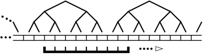
Figure 2: Translational averaging using the moving window technique.

3 Restoring translational invariance

Before the above theoretical cumulants can be compared to experimentally measured ones, the issue of translational invariance must be dealt with. Clearly, the generating function (2) and its cumulants (2) are not translationally invariant, in conflict with the homogeneous statistics characterising experimental results. Spatially homogeneous statistics can, however, be emulated by creating a theoretical time series consisting of a chain of $m$ adjacent independent cascade fields with $2^{J}$ finest-scale bins each [9]. In analogy to the experimental situation, an observation window of width $2^{J}\eta$ is successively moved over this series in bin-sized steps, $t=1,\ldots,(m-1)2^{J}$, successively “seeing” parts of adjacent cascade configurations: see Figure 2.

A translationally invariant one-point moment density would thus be constructed as

$$\overline{\rho}_{n}=\lim_{m\rightarrow\infty}\;{1\over(m-1)\,2^{J}}\sum_{t=1}^{(m-1)2^{J}}\left(\ln\varepsilon_{t}\right)^{n}\,,$$ (10)

which should be comparable to the experimental time series. Operationally, this can be implemented by keeping only one cascade while averaging over many different cascade configurations, i.e. 

$$\overline{\rho}_{n}={1\over M}\sum_{t=1}^{M}\left\langle(\ln\varepsilon_{t})^{n}\right\rangle={1\over M}\sum_{t=1}^{M}\rho_{n}(t)\,,$$ (11)

with $M\equiv 2^{J}=L/\eta$ and $\langle\;\rangle$ denoting configuration averaging. Likewise, a translationally invariant two-point density with constant distance $\eta\,d$ (with $d=1,2,3,\ldots$) between the two bins would be simulated by two adjacent cascades,

$$\overline{\rho}_{r,s}(d)={1\over M}\sum_{t=1}^{M}\rho_{r,s}(t,t{+}d)\,,$$ (12)

with $\rho_{r,s}(t,t{+}d)=\left\langle(\ln\varepsilon_{t})^{r}(\ln\varepsilon_{t+d})^{s}\right\rangle$. As shown in Figure 3, bin $t{+}d$ at some stage in the summation exceeds $M=2^{J}$ and hence would refer to the right-hand cascade while $t$ would refer to the left-hand one.

Figure 3: Translational averaging for two-point statistics. Indices $t$ and $t{+}d$ run over all bins with the “euclidean distance” $d$ kept fixed.

Given that the model provides solutions in terms of cumulants, it is tempting to apply this averaging prescription directly to cumulants also, i.e. to define

$$\overline{C}_{r,s}(d)={1\over M}\sum_{t=1}^{M}C_{r,s}(t,t{+}d)\,,$$ (13)

using for $C_{r,s}(t,t{+}d)$ theoretical expressions obtained from (2). However, experimental cumulants are derived from measured moments rather than the other way round [10] (for example $C_{2}\equiv\rho_{2}-\rho_{1}^{2}$, $C_{3}\equiv\rho_{3}-3\rho_{2}+2\rho_{1}^{3}$), so that averaging over moments rather than cumulants is mandatory for theory also. The proper procedure is hence to convert theoretical cumulants (2) to moments, average these over $t$, and then convert these back to cumulants for experimental comparison.

For the one-point case, this convoluted route becomes simple: the $n$-th order one-point cumulant $C_{n}(t)\equiv C(\kappa_{1}{=}\ldots{=}\kappa_{n}{=}t)$, given by

$$C_{n}(t)=Jc_{n}\,,$$ (14)

is independent of position $t$ so that translational averaging is trivial. The only remaining complication is that $J$ is not an experimental observable, and this is easily addressed by looking at cumulant ratios $C_{n}/C_{n^{\prime}}$ for which the $J$-dependence cancels. Ratios of translationally averaged one-point cumulants,

$${\overline{C}_{n}\over\overline{C}_{n^{\prime}}}={c_{n}\over c_{n^{\prime}}}={\langle\left(\ln q\right)^{n}\rangle_{c}\over\langle\left(\ln q\right)^{n^{\prime}}\rangle_{c}}\;,$$ (15)

being independent of $J$, should hence be directly comparable to experiment.

To demonstrate the quality of these cumulant ratios, we consider three model distributions, all with factorised splitting function

$$p(q_{L},q_{R})=p(q_{L})\,p(q_{R})\,,$$ (16)

namely a binomial distribution (often also termed the “$\alpha$ model”),

$$p(q) = {\alpha_{2}\over{\alpha_{1}+\alpha_{2}}}\;\delta\left(q-(1-\alpha_{1})\right)$$ (17)

$$+ {\alpha_{1}\over{\alpha_{1}+\alpha_{2}}}\;\delta\left(q-(1+\alpha_{2})\right)\,,$$

with parameters $\alpha_{1}=0.3$ and $\alpha_{2}=0.65$, a log-normal distribution

$$p(q)={1\over\sqrt{2\pi}\;\sigma q}\exp\left[-{1\over 2\sigma^{2}}\left(\ln q+\frac{\sigma^{2}}{2}\right)^{2}\right]$$ (18)

with parameter $\sigma=0.42$, and a beta distribution

$$p(q)={\Gamma(\beta_{1}+\beta_{2})\over\Gamma(\beta_{1})\Gamma(\beta_{2})}\,8^{1-\beta_{1}-\beta_{2}}\,q^{\beta_{1}-1}\,(8-q)^{\beta_{2}-1}$$ (19)

with parameters $\beta_{1}=4.88=\beta_{2}/7$ and $q\in(0,8)$. The beta model is particularly appealing because it parallels the experimental situation where energy conservation in three dimensions results in a non-energy-conserving one-dimensional projection. Parameter values quoted are the result of requiring $\langle q\rangle=1$ and best fits needed to reproduce observed multiplier statistics [2], which hence cannot distinguish between these three models.

Figure 4: Multifractal scaling exponents $\tau(n)$ for the binomial (circles, eq. (17)), lognormal (squares, eq. (18)) and beta (diamonds, eq. (19)) distributions.

Figure 5: Same-lineage cumulants $c_{n}$ for the binomial (circles, eq. (17)), lognormal (squares, eq. (18)) and beta (diamonds, eq. (19)) distributions.

As shown in Figure 4, all three splitting functions also have almost identical multifractal scaling exponents $\tau(n)=\ln\langle q^{n}\rangle/\ln 2$. Since $\langle q\rangle=1$ by construction, $\tau(1)$ is zero for all three distributions. For $n=2$ we get $\tau(2)=0.26$ for the first two distributions and $0.23$ for the beta distribution, indistinguishable within the uncertainty of the experimental intermittency exponent $\mu=0.25\pm 0.05$ [11]. We secondly note that even for $n\geq 3$ the $\tau(n)$’s for the binomial and the beta distributions remain indistinguishable. Thirdly, all three distributions have a positive skewness $\langle(q-\langle q\rangle)^{3}\rangle/\langle(q-\langle q\rangle)^{2}\rangle^{3/2}$ when measured in $q$ and reproduce the observed multiplier statistics, including their correlations. This has been shown for the binomial and log-normal in Ref. [4]. Numerical analysis of the beta distribution yields similar results. Fits to observed scaling exponents have not been performed because it is not straightforward to compare theoretical and experimental scaling exponents due to the finiteness of the inertial range [12].

The above observables thus fail manifestly to distinguish between the different model distributions. By contrast, Figure 5 demonstrates that, while $c_{1}$ and $c_{2}$ are almost identical for the three models, higher-order cumulants and cumulant ratios (15) are very different. For example, $c_{3}=0.05$, $0.00$ and $-0.05$ for the distributions (17), (18) and (19) respectively, so that the theoretical cumulant ratios

$${\overline{C}_{3}\over\overline{C}_{2}} = {c_{3}\over c_{2}}\;=\;{\left\langle(\ln q)^{3}\right\rangle_{c}\over\left\langle(\ln q)^{2}\right\rangle_{c}}$$ (20)

$$= \left\{\begin{array}[]{rl}0.31&\qquad{\rm(binomial)}\\ 0.00&\qquad{\rm(lognormal)}\\ -0.25&\qquad{\rm(beta)}\end{array}\right.$$ (24)

lead to results that differ even in sign. If the present model assumptions are adequate, this sign difference should be seen in the experimental ratio

$${\overline{C}_{3}^{\rm obs}\over\overline{C}_{2}^{\rm obs}}={\langle(\ln\varepsilon)^{3}\rangle-3\langle(\ln\varepsilon)^{2}\rangle\langle\ln\varepsilon\rangle+2\langle\ln\varepsilon\rangle^{3}\over\langle(\ln\varepsilon)^{2}\rangle-\langle\ln\varepsilon\rangle^{2}}\,.$$ (25)

In fourth order, the same-lineage cumulant $c_{4}$ has a different sign for the binomial and beta distribution, so that the ratios $\overline{C}_{4}/\overline{C}_{2}=c_{4}/c_{2}$ of two-point cumulants come with a different sign, too. For the log-normal distribution, these ratios are of course again zero.

Figure 6: Some examples for the ultrametric distance $D$ in a cascade with $J=3$.

4 Two-point cumulants and geometry

Having demonstrated the advantages of measuring ratios of one-point cumulants, we now consider equivalent two-point ratios. The theoretical two-point cumulant for two bins is found in terms of their mutual ultrametric distance $D>0$. As illustrated [7] in Figure 6, two bins $\kappa_{1}=(k_{1}\cdots k_{j}k_{j+1}\cdots k_{J})$ and $\kappa_{2}=(k_{1}\cdots k_{j}k_{j+1}^{\prime}\cdots k_{J}^{\prime})$, with $k_{j+1}\neq k_{j+1}^{\prime}$, are separated by an ultrametric distance $D=J-j$.

$$C_{r,s}(D)=(J-D)c_{r+s}+c_{r,s}\;.$$ (26)

Again we must restore translational invariance using (12) for theoretical densities $\rho_{r,s}$ rather than (13) for cumulants. In doing so, we must note that, since the density $\rho_{r,s}(t,t{+}d)$ factorises when bins $t$ and $t+d$ belong to independent cascades, i.e. whenever $M-d+1\leq t\leq M$, the averaged moment splits up,

$$\overline{\rho}_{r,s}(d) = {1\over M}\sum_{t=1}^{M-d}\rho_{r,s}(t,t+d)$$ (27)

$$+ {1\over M}\sum_{t=M-d+1}^{M}\rho_{r}(t)\rho_{s}(t+d)\,.$$

Analytic expressions for $\rho_{r,s}(t,t+d)$ are again readily derived by inserting the cumulants (14) and (26) into the usual relations between $n$-variate moments and cumulants [10] and thence into (27).

Since the cumulants $c_{n}$ and $c_{r,s}$ are independent of $t$, this procedure clearly involves summation of $(J-D)$ over $t$ as in (26) to create “geometrical coefficients” of $c_{n}$ and $c_{r,s}$ of the type

$$G_{n}(J,d)={1\over M}\sum_{t=1}^{M-d}\left(J-D(t,t+d)\right)^{n}$$ (28)

with $n=0,1,2,\ldots$, where the dependence of the ultrametric distance $D$ on the bin positions is made explicit. These coefficients are best evaluated by changing the index of of summation,

$$G_{n}(J,d)=\sum_{D=1}^{J}p(D|J,d)\,(J-D)^{n}\;,$$ (29)

with $p(D|J,d)$ the (normalised) histogram function counting the number of times $D$ appears while $t$ runs over its allowed values. Empirically, we find

$$p(D|J,d)=\left\{\begin{array}[]{lrl}0&(1\leq D<A)&\\ 1-(d/2^{A})&(D=A)&\\ d/2^{D}&(A<D\leq J)&,\end{array}\right.$$ (30)

where $A=\lceil\log_{2}d\rceil$ is the ceiling of $\log_{2}d$. Insertion of (30) into (29) leads to analytical expressions for the geometrical coefficients

$$G_{0}(J,d) = (1-2^{-J}d)\;,$$ (31)

$$G_{1}(J,d) = (J-A)-2d(2^{-A}-2^{-J})\;,$$ (32)

$$G_{2}(J,d) = (J-A)^{2}-4d(J-A)2^{-A}$$ (33)

$$+ 6d(2^{-A}-2^{-J})\,,$$

which in turn yield analytical results for the averaged two-point densities $\overline{\rho}_{r,s}(d)$ of (27). Spatially homogeneous two-point cumulants are then constructed via the inversion formulae [10]

$$\overline{C}_{1,1}(d) = \overline{\rho}_{1,1}(d)-\overline{\rho}_{1}^{2}\,,$$ (34)

$$\overline{C}_{2,1}(d) = \overline{\rho}_{2,1}(d)-2\overline{\rho}_{1}\overline{\rho}_{1,1}(d)$$ (35)

$$-\;\overline{\rho}_{2}\overline{\rho}_{1}+2\overline{\rho}_{1}^{3}\,,$$

$$\overline{C}_{3,1}(d) = \overline{\rho}_{3,1}(d)-3\overline{\rho}_{1}\overline{\rho}_{2,1}(d)-\overline{\rho}_{3}\overline{\rho}_{1}$$ (36)

$$-\;3\overline{\rho}_{2}\overline{\rho}_{1,1}(d)+6\overline{\rho}_{1}^{2}\overline{\rho}_{1,1}(d)$$

$$+\;6\overline{\rho}_{2}\overline{\rho}_{1}^{2}-6\overline{\rho}_{1}^{4}\,,$$

$$\overline{C}_{2,2}(d) = \overline{\rho}_{2,2}(d)-4\overline{\rho}_{1}\overline{\rho}_{2,1}(d)-2(\overline{\rho}_{1,1}(d))^{2}$$ (37)

$$-\;\overline{\rho}_{2}^{2}+8\overline{\rho}_{1}^{2}\overline{\rho}_{1,1}(d)$$

$$+\;4\overline{\rho}_{2}\overline{\rho}_{1}^{2}-6\overline{\rho}_{1}^{4}\,.$$

With Eqs. (27)–(33), we arrive for $s{=}1$ at

$$\overline{C}_{r,1}(d)=G_{1}(J,d)\,c_{r{+}1}+G_{0}(J,d)\,c_{r,1}\,.$$ (38)

This turns out to be equivalent to direct translational averaging of cumulants (13). For $s{\neq}1$, however, such direct averaging is wrong and the full conversion from cumulant to moment to averaged moment and back to averaged cumulant is unavoidable. For $r{=}s{=}2$ we get, for example,

$$\overline{C}_{2,2}(d) = G_{2}(J,d)c_{2}^{2}+G_{1}(J,d)\left(c_{4}+4c_{2}c_{1,1}\right)$$ (39)

$$+ G_{0}(J,d)\left(c_{2,2}+2c_{1,1}^{2}\right)$$

$$- 2\left[G_{1}(J,d)c_{2}+G_{0}(J,d)c_{1,1}\right]^{2}\,,$$

where the additional terms are a consequence of the third term in the expression (37) for $\overline{C}_{2,2}(d)$. Averaged two-point cumulants $\overline{C}_{r,s}$ of higher order $r,s{\geq}2$ exhibit similar structures. Translationally averaged $n$-point cumulants $\overline{C}_{m_{1},\ldots,m_{n}}$ can be calculated by the procedure sketched above.

Figure 7 shows explicit examples for $G_{0}$ and $G_{1}$ for a cascade of length $J=5$. As expected, $G_{0}$ reflects the trivial dependence of the splitting cumulant on the sum limits $1\leq t\leq M{-}d$, apart from the point $d{=}0$ for which no splitting cumulant enters at all. More interesting is the coefficient for the same-lineage cumulant, $G_{1}$: it consists of a series of straight-line segments, changing slope whenever $d\,\textrm{mod}\,2=0$ and ending at zero for $d\geq 2^{J}/2$. Since the form of $G_{1}$ changes whenever $d$ is a power of 2, approximate exponential behaviour of $\overline{C}_{r,1}$ as a function of $d$ is to be expected; this is shown in Figure 8. The exponential form would, however, be destroyed by any sizeable contribution of $G_{0}$ entering via the splitting cumulant, especially at larger $d$.

The form of $G_{1}$ can be further understood by considering an alternative formulation for $p(D|J,d)$ in terms of $k=\lfloor\log_{2}d\rfloor$,

$$p(D|J,d) = (1-d2^{-J})\delta_{J-D}$$

$$+ \sum_{j=1}^{J-1}\Theta(J-j-k)\;(1-2^{j-J}\,d)$$

$$\qquad\times(\delta_{J-D-j}-\delta_{J-D-j+1})\,,$$

(with $\delta_{n}=\delta_{n,0}$ the Kronecker delta and $\theta(n)=0$ whenever $n\leq 0$ and 1 otherwise) since, with $G_{1}=\sum_{D=1}^{J}(J-D)\,p(D|J,d)$, we find

$$G_{1}(J,d)=\sum_{j=1}^{J-1}\Theta(2^{J-j}-d)\;(1-2^{j-J}\,d)\,,$$ (41)

which is a sum of straight-line contributions kicking in whenever $d$ becomes smaller than $2^{J-j},j=1,2,\ldots$ This means that whenever $d$ becomes smaller than some dyadic fraction of $M$, the two bins $t$ and $t{+}d$ can fall within the same $(J{-}j)$-scale subcascade so that $G_{1}$ picks up new contributions from this scale.

Figure 7: Geometrical coefficients $G_{1}$ and $G_{0}$, on linear scale for $J{=}5$.

Translationally invariant cumulants $\overline{C}_{r,s}$ are constructed from these factors according to eqs. (38)–(39). Figure 9 shows by example $\overline{C}_{1,1}$ for the binomial ($\alpha$ model) and the corresponding energy-conserving $p$-model with pdf

$$p(q_{L},q_{R}) = \left[\textstyle{1\over 2}\delta(q_{L}-1-\alpha)+\textstyle{1\over 2}\delta(q_{L}-1+\alpha)\right]$$

$$\;\times\;\delta(q_{L}+q_{R}-2)\,,$$

setting (for purposes of comparison) $\alpha_{1}=\alpha_{2}=\alpha=0.4$. The $\alpha$-model has $c_{r,s}=0$ and hence contains no contribution from $G_{0}$ but only from $G_{1}$ and $c_{2}=\textstyle{1\over 4}\left[\ln\left((1+\alpha)/(1-\alpha)\right)\right]^{2}=0.1795$, while for the $p$-model both $c_{1,1}={-}c_{2}$ and $c_{2}$ contribute in (38). The resulting $p$-model $\overline{C}_{1,1}$ has the same peak at $d{=}0$ as the $\alpha$-model but exhibits the familiar anticorrelation (negative cumulant) at larger $d$ [13]. Whether and for what $d$ the $\overline{C}_{1,1}$ is negative depends, however, on the sum of same-side and splitting cumulant contributions rather than on the splitting cumulant alone.

Figure 8: Geometrical coefficients $G_{1}$ and $G_{0}$, on logarithmic scale for $J{=}5$ and $J{=}10$, showing the approximately exponential behaviour of $G_{1}$.

Figure 9: $C_{1,1}$ two-point cumulants for the binomial and $p$-models with $J=5$, showing contributions from same-lineage and splitting parts of the respective splitting functions. Solid lines represent the (scaled) geometrical coefficients.

We further note that all models whose splitting function factorises have zero translationally invariant two-point cumulants for $d\geq 2^{J}/2$. Roughly, this can be translated into the statement that deviations of two-point cumulants from zero for “long” distances $d$ (compared to an admittedly fluctuating cascade size which we have modelled as a constant $2^{J}$) would signal the nonfactorisation of the splitting function and vice versa.

Returning to cumulant ratios, we focus on cumulants $\overline{C}_{r,1}(d)$. If the splitting function factorises as in (16), then the splitting cumulant $c_{r,s}$ is zero and the two-point cumulant for $d\geq 1$, becomes directly proportional to the geometrical coefficient $G_{1}(J,d)$,

$$\overline{C}_{r,1}(d)=c_{r{+}1}\,G_{1}(J,d)\,.$$ (42)

Taking ratios of two-point cumulants of different orders,

$${\overline{C}_{r,1}(d)\over\overline{C}_{r^{\prime},1}(d)}={c_{r{+}1}\over c_{r^{\prime}{+}1}}={\langle(\ln q)^{r+1}\rangle_{c}\over\langle(\ln q)^{r^{\prime}+1}\rangle_{c}}\;,$$ (43)

the geometrical coefficient drops out, so that these ratios become independent of $d$. This is an important observation as it grants access to properties of the pdf (cascade generator) even after spatial homogeneity has been restored. Also, the $d$-independence of these ratios constitutes a severe test of the model assumptions entering the cascade models. Furthermore, the factorisation assumption can be tested since one- and two-point ratios are equal if (16) holds,

$${\overline{C}_{r,1}(d)\over\overline{C}_{r^{\prime},1}(d)}={c_{r{+}1}\over c_{r^{\prime}{+}1}}={\overline{C}_{r+1}\over\overline{C}_{r^{\prime}+1}}\quad\forall\;d\;.$$ (44)

In this case, ${\overline{C}_{2,1}/\overline{C}_{1,1}}$ would assume the same numerical values as those in Eq. (20), with similar powers to discriminate between models. Two-point cumulant ratios would hence also predict clearly different results, in contrast with scaling exponents and multiplier distributions.

We also note that the connection [6] between the multifractal scaling exponents $\tau(n{=}\lambda)$ and the cumulant branching generating function (6),

$$\tau(\lambda)={\ln\left\langle q^{\lambda}\right\rangle\over\ln 2}={Q(\lambda,0)\over\ln 2}\;,$$ (45)

implies that the same-lineage cumulants (8), which are to be extracted from ratios (15) or (42), are related to the $\tau(n)$ by

$$c_{n}=\left.{\partial^{n}Q(\lambda,0)\over\partial\lambda^{n}}\right|_{\lambda=0}=\left.\ln 2\;{\partial^{n}\tau(\lambda)\over\partial\lambda^{n}}\right|_{\lambda=0}\;,$$ (46)

i.e. the cumulant $c_{n}$ in $\ln q$ is related to the $n$-th derivative of the scaling exponent $\tau(\lambda)$, taken at $\lambda=0$. In principle, this not only allows for an unambiguous, albeit indirect extraction of scaling exponents, but also of the more fundamental splitting function.

We end on an interesting sideline regarding the detection of scaling in the bin size $\ell$. Conventionally, this is done by plotting $\ln\langle\varepsilon^{n}\rangle$ against $\ln\ell$ in the expectation of seeing a straight line. The same scaling of $\langle\varepsilon^{n}\rangle$ is just as easily detected by pointing out that the one-point cumulant in $\ln\varepsilon$ is given at every scale $j$ by $\overline{C}_{n}^{(j)}=jc_{n}$ and, since $\ell_{j}/L=2^{-j}$,

$$\overline{C}_{n}^{(j)}={\ln(L/\ell_{j})\over\ln 2}\;c_{n}\;;$$ (47)

in other words, scaling in $\langle\varepsilon^{n}\rangle$ is manifest in a logarithmic dependence on the length scale $\ell_{j}$ of the corresponding one-point cumulant in $\ln\varepsilon$. It must be remembered, though, that such “forward” scaling behaviour can be destroyed by the processes of translational averaging as well as the experimental “backward” box summation [13].

5 Discussion

We have shown that features of the analytical solution for cumulants in $\ln\varepsilon$ can be preserved beyond the complication of translational invariance, and in the process elucidated the interplay between the same-lineage and splitting cumulants generated at each cascade splitting on the one hand, and the geometrical features on the other. We are, of course, tempted to apply two-point cumulants of $\ln\varepsilon$ directly to the experimental energy dissipation field deduced from hot-wire time series and to study possible dependences on the Reynolds number and the flow configuration. This may be done in the spirit of naive discovery. We do think, however, that studies of different model assumptions such as continuous multiplicative cascade processes [14], hierarchical shell models [15], effects of finite inertial range etc. should sensibly be undertaken before taking the comparison with data too seriously.

Acknowledgements:
We thank Jürgen Schmiegel for fruitful discussions. This work was funded in part by the South African National Research Foundation. HCE thanks the organisers of this workshop and the MPIPKS for kind hospitality and support.

References

- [1] A.S. Monin and A.M. Yaglom, Statistical Fluid Mechanics, Vol. 1 and 2, (MIT Press, Cambridge, 1971); U. Frisch, Turbulence (Cambridge University Press, Cambridge, 1995).
- [2] K.R. Sreenivasan and G. Stolovitzky, J. Stat. Phys. 78, 311 (1995); G. Pedrizzetti, E.A. Novikov and A.A. Praskovsky, Phys. Rev. E53, 475 (1996).
- [3] B. Jouault, P. Lipa and M. Greiner, Phys. Rev. E59, 2451 (1999).
- [4] B. Jouault, M. Greiner and P. Lipa, Physica D136, 125 (2000); B. Jouault, J. Schmiegel and M. Greiner, chao-dyn/9909033.
- [5] A. Naert, R. Friedrich and J. Peinke, Phys. Rev. E56, 6719 (1997); P. Marcq and A. Naert, Physica D134, 368 (1998); J. Cleve and M. Greiner, nlin.CD/0003044.
- [6] M. Greiner, H.C. Eggers and P. Lipa, Phys. Rev. Lett. 80, 5333 (1998); M. Greiner, J. Schmiegel, F. Eickemeyer, P. Lipa, and H.C. Eggers, Phys. Rev. E58, 554 (1998).
- [7] H.C. Eggers, M. Greiner and P. Lipa, in: Correlations and Fluctuations ’98, 8th International Workshop on Multiparticle Production, Mátraháza, edited by T. Csörgő, S. Hegyi, R.C. Hwa and G. Jancsó, World Scientific (1999) pp. 264–271.
- [8] H.C. Eggers and M. Greiner, to be published.
- [9] M. Greiner, J. Giesemann and P. Lipa, Phys. Rev. E56, 4263 (1997).
-
[10]
P. Carruthers, H.C. Eggers and I. Sarcevic,
Phys. Lett. B254, 258 (1991);
A. Stuart and J.K. Ord, Kendall’s Advanced Theory of Statistics, Volume 1, 5th Edition, Oxford University Press, New York (1987). - [11] K.R. Sreenivasan and R.A. Antonia, Ann. Rev. Fluid Mech. 29, 435 (1997).
- [12] J. Schmiegel, B. Jouault, J. Cleve, T. Dziekan and M. Greiner, in preparation.
- [13] M. Greiner, J. Giesemann, P. Lipa and P. Carruthers, Z. Phys. C69, 305 (1996).
- [14] D. Shertzer, S. Lovejoy, F. Schmitt, Y. Chigirinskaya, and D. Marsan, Fractals 5, 427 (1997).
- [15] R. Benzi, L. Biferale, R. Tripiccione and E. Trovatore, Phys. Fluids 9, 2355 (1997); R. Benzi, L. Biferale and E. Trovatore, Phys. Rev. Lett. 79, 1670 (1997).