CP-violating $ZZh$ Coupling at $e^{+}e^{-}$ Linear Colliders

Abstract

We study the general Higgs-weak boson coupling with CP-violation via the process $e^{+}e^{-}\to f\bar{f}h$. We categorize the signal channels by sub-processes $Zh$ production and $ZZ$ fusion and construct four CP asymmetries by exploiting polarized $e^{+}e^{-}$ beams. We find complementarity among the sub-processes and the asymmetries to probe the real and imaginary parts of the CP-violating form factor. Certain asymmetries with unpolarized beams can retain significant sensitivity to the coupling. We conclude that at a linear collider with high luminosity, the CP-odd $ZZh$ coupling may be sensitively probed via measurements of the asymmetries.

I Introduction

Searching for a Higgs boson has been a major motivation for many current and future collider experiments, since Higgs bosons encode the underlying physics of mass generation. In the minimal Standard Model (SM), there is only one CP-even scalar. In the two-Higgs doublet model or the supersymmetric extension of the SM, there are two CP-even states, one CP-odd state, plus a pair of charged Higgs bosons. The couplings of Higgs bosons to electroweak gauge bosons are particularly important since they faithfully represent the nature of the electroweak gauge symmetry breaking. Determining the detailed properties of the Higgs boson couplings will be of fundamental importance to fully construct the theoretical framework of the electroweak sector.

FIG. 1.: Vertex function for $ZZh$ coupling.

The most general interaction vertex for a generic Higgs boson ($h$) and a pair of $Z$ bosons, $Z^{\mu}(k_{1})\ Z^{\nu}(k_{2})\ h$, can be expressed by the following Lorentz structure

$$\Gamma^{\mu\nu}(k_{1},k_{2})=i{2\over v}\ h\ [a\ M_{Z}^{2}g^{\mu\nu}+b\ (k_{1}^{\mu}k_{2}^{\nu}-k_{1}\cdot k_{2}g^{\mu\nu})+\tilde{b}\ \epsilon^{\mu\nu\rho\sigma}k_{1\rho}k_{2\sigma}],$$ (1)

where $v=(\sqrt{2}G_{F})^{-1/2}$ is the vacuum expectation value of the Higgs field, and the $Z$ boson four-momenta are both incoming, as depicted in Fig. 1. The $a$ and $b$ terms are CP-even and the $\tilde{b}$ term is CP-odd. Thus, the simultaneous existence of terms $a$ (or $b$) and $\tilde{b}$ would indicate CP violation for the $ZZh$ coupling [1, 2, 3]. We note that in the SM at tree level, $a=1$ and $b=\tilde{b}=0$. In supersymmetric theories with CP-violating soft SUSY breaking terms [4], these CP-violating interactions may be generated by loop diagrams. More generally, the parameters can be momentum-dependent form factors and of complex values to account for the dispersive [${\cal R}\!e(\tilde{b}$)] and absorptive [${\cal I}\!m(\tilde{b}$)] effects from radiative corrections. Alternatively, in terms of an effective Lagrangian, the $b$ term can be from gauge invariant dimension-6 operators [5], and the $\tilde{b}$ term can be constructed similarly with CP-odd operators involving the dual field tensors. Dimensional analysis implies that the parameters $b$ and $\tilde{b}$ may naturally be of the order of $(v/\Lambda)^{2}$ where $\Lambda$ is the scale at which the physics responsible for the electroweak symmetry breaking sets in, presumably $\Lambda\mathrel{\raise 1.29167pt\hbox{$<$\kern-7.5pt\lower 4.30554pt\hbox{$\sim$}}}4\pi v$. The CP-odd coefficient $\tilde{b}$ is of course very much model-dependent.

Possible CP-violation effects via Higgs-gauge boson couplings have recently drawn a lot of attention in the literature. In Ref. [1], CP-odd observables in decays $h\to ZZ,W^{+}W^{-}$ and $t\bar{t}$ were constructed. It was discussed extensively how to explore the Higgs properties via the process $e^{+}e^{-}\to Zh$ [2, 3] at future linear colliders. The polarized photon-photon collisions for $\gamma\gamma\to h$ [6] and the electron-electron scattering process $e^{-}e^{-}\to e^{-}e^{-}h$ [7] were also considered to extract the CP-violating couplings. There has also been considerable amount of work for investigation of CP-violating Higgs boson interactions with fermions at future $e^{+}e^{-}$ colliders [8].

In this paper, we study the CP-violating coupling of $ZZh$ at future $e^{+}e^{-}$ linear colliders. In Section II, we set out the general consideration, identifying the $Zh$ production and $ZZ$ fusion signals and exploring the generic CP-odd variables by exploiting the polarized beams. Given specific kinematics of the signal processes under investigation, we construct four CP asymmetries in Section III. We find important complementarity among the sub-processes and the asymmetries in probing different aspects of the CP-odd coupling, namely the real (dispersive) and imaginary (absorptive) parts of $\tilde{b}$. We also examine to what extent this coupling can be experimentally probed via measurements of the CP asymmetries, with and without beam polarization. We present some general discussions of our analyses and summarize our results in Section IV.

II General consideration

We concentrate on the scenario with a light Higgs boson below the $W$-pair threshold. The Higgs-weak boson coupling will be studied mainly via Higgs production, rather than its decay. We focus on the Higgs boson production associated with a fermion pair in the final state

$$e^{-}(p_{1})\ e^{+}(p_{2})\to f(q_{1})\ \bar{f}(q_{2})\ h(q_{3}).$$ (2)

The Higgs boson signal may be best identified by examining the recoil mass variable

$$m_{rec}^{2}=(p_{1}+p_{2}-q_{1}-q_{2})^{2}=s+m_{ff}^{2}-2{\sqrt{s}}(E_{f}+E_{\bar{f}}),$$ (3)

where $m_{ff}$ is the $f\bar{f}$ invariant mass and $E_{f}\ (E_{\bar{f}})$ is the fermion (anti-fermion) energy in the c. m. frame. This recoil mass variable will yield a peak for the signal at the Higgs mass $m_{h}$, independent of the Higgs decay. This provides a model-independent identification for the Higgs signal. For this purpose, we will accept only

$$f=e^{-},\ \mu^{-}\quad{\rm and}\quad u,\ d,\ s$$ (4)

to assure good energy determination for the final state leptons and light quark jets. Whenever appropriate, we adopt energy smearing according to a Gaussian distribution as

$${\Delta E\over E} = {12\%\over\sqrt{E}}\oplus 1\%\qquad{\rm for\ leptons}$$ (5)

$$= {45\%\over\sqrt{E}}\oplus 2\%\qquad{\rm for\ quarks}.$$ (6)

In realistic experimentation, the charged tracking information may also be used to help improve the momentum determination.

As an illustration, the recoil mass spectrum for an $e^{+}e^{-}$ final state is shown in Fig. 2 by the dashed curve. The width of the peak in $m_{rec}$ spectrum is determined by the energy resolution of the detector as simulated with Eq. (5). We have also required the final state fermions to be within the detector coverage, assumed to be

$$|\cos\theta_{f}|<\cos 10^{\circ}$$ (7)

with respect to the beam hole.

FIG. 2.: Normalized mass distributions for $e^{+}e^{-}\to e^{+}e^{-}h$ at $\sqrt{s}=500\ \rm GeV$ with $m_{h}=120\ \rm GeV$. The dashed curve is for the recoil mass in Eq. (3), and the solid is for the invariant mass $m_{ee}$.

A $Zh$ production versus $ZZ$ fusion

The signal channel Eq. (2) can be approximately divided into two sub-processes

$$e^{+}e^{-}\to Zh\qquad(Zh\ {\rm production})~{},$$ (8)

$$Z^{*}Z^{*}\to h\qquad(ZZ\ {\rm fusion}).$$ (9)

Eq. (8) yields light fermion states of all flavors from $Z$ decay; while Eq. (9) always has an $e^{+}e^{-}$ pair in the final state. These two sub-processes can be effectively distinguished by identifying the final state fermions. Even for the final state of $e^{+}e^{-}$, one can separate them by examining the mass spectrum $m_{ee}$. This is illustrated in Fig. 2 for the $e^{+}e^{-}$ final state by the solid curve. The sharp peak at $M_{Z}$ indicates the contribution from the decay $Z\to e^{+}e^{-}$, while the continuum spectrum at higher mass values is from $ZZ$ fusion sub-process. In our analysis, we have included both contributions coherently. However, when necessary, we separate out the $ZZ$ fusion contribution by requiring

$$m_{ee}>100\ \rm GeV.$$ (10)

FIG. 3.: Total cross sections for $e^{+}e^{-}\to e^{+}e^{-}h$ in fb (a) versus $\sqrt{s}$ for representative values of $m_{h}$, and (b) versus $m_{h}$ for representative values of $\sqrt{s}$. The dashed curves are for $e^{+}e^{-}\to Zh\to e^{+}e^{-}h$ only. No kinematical cuts are imposed.

The $Zh$ associated production is the leading channel for Higgs boson searches at $e^{+}e^{-}$ colliders. $ZZ$ fusion, on the other hand, is often thought to be much smaller due to the small $Z\bar{e}e$ vector coupling and low radiation rate of $Z$ bosons off $e^{\pm}$ beams. However, the rate of the fusion process increases with c. m. energy logarithmically like $\ln^{2}(s/M_{Z}^{2})$, and it is also more important for higher Higgs masses. The $ZZ$ fusion process naturally leads to a pair of electrons in the final state, which is desirable when the charge information of the final state is needed. Moreover, due to the helicity conservation at high energies, the $Zh$ production has only helicity combinations for the initial $e^{+}e^{-}$ of $(+-)$ and $(-+)$; while the $ZZ$ fusion has $(--)$ and $(++)$ in addition, where $-\ (+)$ refers to the left (right) handed helicity. These additional helicity amplitudes may provide further information regarding the CP test, as we will see in the later analysis.

Figure 3 presents the total cross sections for $e^{+}e^{-}\to e^{+}e^{-}h$ to demonstrate the comparison between the $Zh$ and $ZZ$ fusion processes. Figure 3(a) gives cross sections versus $\sqrt{s}$ for $m_{h}=110-200\ \rm GeV$, and (b) versus $m_{h}$ for $\sqrt{s}=350-800\ \rm GeV$. The solid curves are for the total SM rate including all contributions coherently, and the dashed curves are with a real $Z$ decay for $Zh\to e^{+}e^{-}h$. We see that at $\sqrt{s}=500\ \rm GeV$ and $m_{h}=120\ \rm GeV$, $\sigma(ZZ\to h)\approx 10$ fb$>2\sigma(Zh\to e^{+}e^{-}h,\ \mu^{+}\mu^{-}h)$. At $\sqrt{s}=800\ \rm GeV$ and $m_{h}=120\ \rm GeV$, the fusion cross section becomes about an order of magnitude higher than that of $Zh\to e^{+}e^{-}h,\ \mu^{+}\mu^{-}h$. Clearly, at a linear collider above the $Zh$ threshold, the $ZZ$ fusion process is increasingly more important in studying the Higgs properties [9].

B CP property

To unambiguously identify the effect of CP violation, one needs to construct a “CP-odd variable”, whose expectation value vanishes if CP is conserved [10]. We begin our analysis by examining the CP-transformation property. First of all, we note that the initial state of Eq. (2) can be made a CP eigenstate, given the CP-transformation relation

$$e^{-}(\sigma_{1},\vec{p})\ e^{+}(\sigma_{2},-\vec{p})\Rightarrow e^{-}(-\sigma_{2},\vec{p})\ e^{+}(-\sigma_{1},-\vec{p}),$$ (11)

where $\sigma_{i}$ is the fermion helicity. Now consider a helicity matrix element ${\cal M}_{\sigma_{1}\sigma_{2}}(\vec{q}_{1},\vec{q}_{2})$ where $\sigma_{1}\ (\sigma_{2})$ denotes the helicity of the initial state electron (positron), which coincides with the longitudinal beam polarization; $\vec{q}_{1}\ (\vec{q}_{2})$ denotes the momentum of the final state fermion (anti-fermion). It is easy to show that under CP transformation,

$${\cal M}_{-+}({\vec{q}_{1}},{\vec{q}_{2}})\Rightarrow{\cal M}_{-+}(-{\vec{q}_{2}},-{\vec{q}_{1}}),$$ (12)

$${\cal M}_{--}({\vec{q}_{1}},{\vec{q}_{2}})\Rightarrow{\cal M}_{++}(-{\vec{q}_{2}},{-\vec{q}_{1}}),$$ (13)

and ${\cal M}_{+-}$, ${\cal M}_{++}$ transform similarly. If CP is conserved in the reaction, Relations (12) and (13) take equal signs. These relations precisely categorize two typical classes of CP test:

CP eigen-process: Under CP, ${\cal M}_{-+}$ (or ${\cal M}_{+-}$) is invariant if CP is conserved. One can thus construct CP-odd kinematical variables to test the CP property of the theory. We can construct a “forward-backward” asymmetry

$${\cal A}^{FB}=\sigma^{F}-\sigma^{B}=\int_{0}^{1}{d\sigma\over d\cos\theta}d\cos\theta-\int_{-1}^{0}{d\sigma\over d\cos\theta}d\cos\theta,$$ (14)

with respect to a CP-odd angular variable $\theta$ . This argument is applicable for unpolarized or transversely polarized beams as well.

CP-conjugate process: ${\cal M}_{--}$ and ${\cal M}_{++}$ are CP conjugate to each other. In this case, instead of a kinematical variable, the appropriate means to examine CP violation is to directly compare the rates of the conjugate processes. We can thus define another CP asymmetry in total cross section rates between the two conjugate processes of opposite helicities, called the “left-right” asymmetry

$${\cal A}_{LR}=\sigma_{--}-\sigma_{++}.$$ (15)

The longitudinally polarized cross section for arbitrary beam polarizations can be calculated by the helicity amplitudes

$$d\sigma(P_{-}P_{+})={1\over 4}[ (1+P_{-})(1+P_{+})d\sigma_{++}+(1+P_{-})(1-P_{+})d\sigma_{+-}$$ (16)

$$+ (1-P_{-})(1+P_{+})d\sigma_{-+}+(1-P_{-})(1-P_{+})d\sigma_{--}],$$ (17)

where $P_{-}\ (P_{+})$ is the electron (positron) longitudinal polarization, with $P_{\pm}=-1\ (+1)$ for purely left (right) handed. Whenever appropriate in our later studies, we will assume the realistic beam polarization as $(|P_{-}|,|P_{+}|)=(80\%,60\%)$ [11].

III CP-odd variables and the CP-odd coupling

In this section, we construct CP-odd variables for the Higgs signal in Eq. (2) in order to study the CP-violating interactions in Eq. (1). Different CP asymmetries appear to be complementary in exploring different aspects of the CP-odd coupling $\tilde{b}$.

A Simple polar angles and ${\cal I}\!m(\tilde{b})$

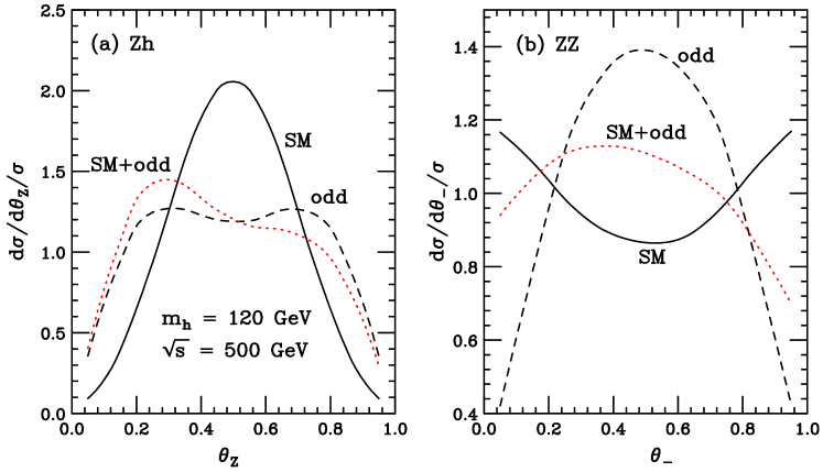
FIG. 4.: Normalized polar angle distributions for $\sigma_{-+}$ at $\sqrt{s}=500\ \rm GeV$ with $m_{h}=120\ \rm GeV$ for (a) $e^{+}e^{-}\to Zh$ with $Z\to f\bar{f}$, and (b) $e^{+}e^{-}\to e^{+}e^{-}h$ via $ZZ$ fusion. The solid curves are for the SM interaction ($a=1$), the dashed for the CP-odd (${\cal I}\!m(\tilde{b})=1$), and the dotted for CP violation with $a={\cal I}\!m(\tilde{b})=1$. $100\%$ longitudinal polarization of $e^{-}_{L}e^{+}_{R}$ has been used.

It has been argued that the $Zh$ process will test the spin-parity property [2] of the coupling by simply measuring the polar angle distribution of the outgoing $Z$ boson. The distribution can be written in the form

$\displaystyle{d\sigma\over d\cos\theta_{Z}}\propto\left\{\begin{array}[]{ll}\beta^{2}\sin^{2}\theta_{Z}+{8M_{Z}^{2}\over s}&\mbox{scalar $h$}\\ 1-{1\over 2}\sin^{2}\theta_{Z}&\mbox{pseudo-scalar $h$}\end{array}\right.$

In fact, this simple polar angle may provide CP information as well. If we rewrite this angle in terms of a dot-product

$$\cos\theta_{Z}={\vec{p}_{1}\cdot\vec{q}_{+}\over|\vec{p}_{1}|\ |\vec{q}_{+}|},$$ (18)

where $\vec{q}_{+}=\vec{q}_{1}+\vec{q}_{2}$ is the vector sum of the outgoing fermion momenta, it is easy to see that it is P-odd and C-even under transformation for the final state. One could thus expect to test CP property of the interactions by examining the polar angle distribution. The experimental study is made particularly simple since this variable does not require charge identification for the final state fermions. Because of this, one expects to increase the statistical accuracy by including some well-measured hadronic decay modes of $Z$, as we accept the light quark jets of Eq. (4). However, after the azimuthal angle integration the dispersive part of the form factor proportional to ${\cal R}\!e(\tilde{b}$) vanishes and the surviving term is the absorptive part proportional to ${\cal I}\!m(\tilde{b}$). The angular distributions are shown in Fig. 4(a) for $\sqrt{s}=500\ \rm GeV$ with $m_{h}=120\ \rm GeV$. The solid curve is for the SM interaction only ($a=1$), the dashed curve is for the CP-odd only (${\cal I}\!m(\tilde{b})=1$), the dotted is for CP violation with $a={\cal I}\!m(\tilde{b})=1$. We see from the dotted curve that there is indeed an asymmetry with respect to the forward ($\pi/2\leq\theta_{Z}\leq 0$) and backward ($\pi\leq\theta_{Z}\leq\pi/2$) regions. We have assumed $100\%$ longitudinal polarization of $e^{-}_{L}e^{+}_{R}$ for illustration here.

FIG. 5.: Forward-backward asymmetries for $\sigma_{-+}$ versus ${\cal I}\!m(\tilde{b})$ at $\sqrt{s}=500\ \rm GeV$ with $m_{h}=120\ \rm GeV$ for (a) $Zh\to f\bar{f}h$: asymmetry in fb, (b) $Zh\to f\bar{f}h$: percentage asymmetry, (c) $ZZ$ fusion: asymmetry in fb, and (d) $ZZ$ fusion: percentage asymmetry. The dashed curves are for $100\%$ longitudinal polarization $e_{L}^{-}e_{R}^{+}$, the solid for a realistic polarization $(e_{L}^{-},e_{R}^{+})=(80\%,60\%)$, and the dotted for unpolarized beams. The error bars are statistical uncertainties obtained with a luminosity of $1000\ \rm fb^{-1}$.

The above calculation can in principle be carried through for the $ZZ$ fusion process. However, due to the unique kinematics in this process, it appears that we can define an alternative polar angle

$$\cos\theta_{-}={(\vec{p}_{1}\times\vec{q}_{-})\cdot(\vec{q}_{1}\times\vec{q}_{2})\over|\vec{p}_{1}\times\vec{q}_{-}|\ |\vec{q}_{1}\times\vec{q}_{2}|},$$ (19)

where $\vec{q}_{-}=\vec{q}_{1}-\vec{q}_{2}$, which yields a larger asymmetry and thus being more sensitive to the coefficient ${\cal I}\!m(\tilde{b}$). It is easy to verify that this variable is P-odd and C-even under transformation for the final state. Figure 4(b) shows the angular distributions for $e^{+}e^{-}\to e^{+}e^{-}h$ via $ZZ$ fusion with $100\%$ longitudinal polarization of $e^{-}_{L}e^{+}_{R}$. The legend is the same as in (a). We see from the dotted curve that an asymmetry exists with respect to this angle.

FIG. 6.: Polarized cross section asymmetry at $\sqrt{s}=500\ \rm GeV$ with $m_{h}=120\ \rm GeV$ versus ${\cal I}\!m(\tilde{b})$ for (a) the asymmetry in fb, and (b) the percentage asymmetry. The dashed curves are for $100\%$ beam polarization, the solid for a realistic polarization $(e^{-},e^{+})=(80\%,60\%)$. The error bars are statistical uncertainties obtained with a luminosity of $1000\ \rm fb^{-1}$.

Replacing $\theta$ by $\theta_{Z}$ in Eq. (14), we can define a forward-backward asymmetry ${\cal A}^{FB}_{\theta_{Z}}$ with respect to the angle $\theta_{Z}$, and similarly another asymmetry ${\cal A}^{FB}_{\theta_{-}}$ with respect to the angle $\theta_{-}$. These two asymmetries are calculated for $\sigma_{-+}$, and shown in Fig. 5 at $\sqrt{s}=500\ \rm GeV$ with $m_{h}=120\ \rm GeV$ versus ${\cal I}\!m(\tilde{b})$. Figures 5(a) and (b) are the asymmetry in fb and the percentage asymmetry respectively, with respect to $\theta_{Z}$ in $Zh\to f\bar{f}h$. Similarly, Figs. 5(c) and (d) show the asymmetry and percent asymmetry for $ZZ$ fusion with respect to $\theta_{-}$. The dashed curves are for $100\%$ longitudinal polarization $e_{L}^{-}e_{R}^{+}$, the solid are for a realistic polarization $(e_{L}^{-},e_{R}^{+})=(80\%,60\%)$, and the dotted are for unpolarized beams. We see that the beam polarization here substantially enhances the asymmetries, and the realistic polarization maintains the asymmetries to a large extent. Some degree of asymmetry still exists even for unpolarized beams. The percentage asymmetry for the $Zh$ process can be as large as $30\%$ for ${\cal I}\!m(\tilde{b})\sim 0.2$, and is typically of a few percent for $ZZ$ fusion.

FIG. 7.: Cross section asymmetries in fb versus $\sqrt{s}$ with $m_{h}=120\ \rm GeV$ for (a) forward-backward asymmetry with respect to $\theta_{Z}$ for ${\cal I}\!m(\tilde{b})=0.1$, (b) forward-backward asymmetry with respect to $\theta_{-}$ for for ${\cal I}\!m(\tilde{b})=0.5$, (c) $LR$ asymmetry between $\sigma_{--}$ and $\sigma-{++}$ for ${\cal I}\!m(\tilde{b})=0.1$. The dashed curves are for $100\%$ longitudinal polarization, and the solid for a realistic polarization $(e^{-},e^{+})=(80\%,60\%)$. The error bars are statistical uncertainties obtained with a luminosity of $1000\ \rm fb^{-1}$.

We wish to address to what extent an asymmetry can be determined by experiments. For this purpose, we estimate the statistical uncertainties for the asymmetry measurements. We determine the Gaussian statistical error by $\sqrt{N_{F}+N_{B}}$ where $N_{F}\ (N_{B})$ is the number of forward (backward) events. The statistical significance for the asymmetry measurement is obtained by

$${|N_{F}-N_{B}|\over\sqrt{N_{F}+N_{B}}}.$$ (20)

The error bars in the plots are calculted with an assumed integrated luminosity of $1000\ \rm fb^{-1}$. Due to the larger asymmetry as well as a larger cross section for $Zh\to f\bar{f}h$, the $Zh$ production would provide a much better determination of ${\cal I}\!m(\tilde{b}$).

As we discussed earlier, the $ZZ$ fusion process can provide another type of asymmetry between CP conjugate processes, in particular between $\sigma_{--}$ and $\sigma_{++}$ as defined in Eq. (15), which is absent in $Zh$ production. This is presented in Fig. 6 for ${\cal A}_{LR}$, at $\sqrt{s}=500\ \rm GeV$ with $m_{h}=120\ \rm GeV$ versus ${\cal I}\!m(\tilde{b})$. Figure 6(a) is the asymmetry in fb. The legend is the same as in Fig. 5. The error bars are for a total integrated luminosity of $1000\ \rm fb^{-1}$ ($500\ \rm fb^{-1}$ each for $\sigma_{--}$ and $\sigma_{++}$). The percentage asymmetry in Fig. 6(b) can be at a $10\%$ level for ${\cal I}\!m(\tilde{b})\sim 0.2$. It is interesting to note that the solid curves yield a non-zero value for $\tilde{b}=0$. This is due to the intrinsic $LR$ asymmetry of the $Z$ coupling to electrons. This shift appears when $|P_{-}|\neq|P_{+}|$ and is proportional to $\sigma_{-+}-\sigma_{+-}$. It can be well predicted in the SM for a given beam polarization.

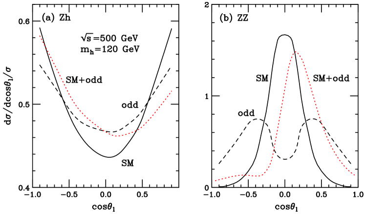
FIG. 8.: Normalized angular distributions for $\sigma_{-+}$ at $\sqrt{s}=500\ \rm GeV$ with $m_{h}=120\ \rm GeV$ for (a) $e^{+}e^{-}\to Zh$ with $Z\to e^{-}e^{+},\mu^{-}\mu^{+}$, and (b) $e^{+}e^{-}\to e^{+}e^{-}h$ via $ZZ$ fusion. The solid curves are for the SM interaction ($a=1$), the dashed for the CP-odd (${\cal R}\!e(\tilde{b})=1$), and the dotted for CP violation with $a={\cal R}\!e(\tilde{b})=1$. $100\%$ longitudinal polarization of $e^{-}_{L}e^{+}_{R}$ has been used.

Cross section asymmetries versus $\sqrt{s}$ are shown in Fig. 7 in units of fb with $m_{h}=120\ \rm GeV$ (a) forward-backward asymmetry for $\sigma_{-+}$ in $Zh$ production with respect to $\theta_{Z}$ for ${\cal I}\!m(\tilde{b})=0.1$, (b) forward-backward asymmetry for $\sigma_{-+}$ in $ZZ$ fusion with respect to $\theta_{-}$ for for ${\cal I}\!m(\tilde{b})=0.5$, (c) $LR$ asymmetry between $\sigma_{--}$ and $\sigma_{++}$ for ${\cal I}\!m(\tilde{b})=0.1$. The dashed curves are for $100\%$ longitudinal polarization, and the solid are for a realistic polarization $(e^{-},e^{+})=(80\%,60\%)$. The error bars are for the statistical uncertainty with a luminosity of $1000\ \rm fb^{-1}$. We see again the possibly good accuracy for determining the asymmetry by the $Zh$ process. Furthermore, these two processes are complementary: at lower energies near threshold the $Zh$ production is far more important; while at higher energies the $ZZ$ fusion becomes increasingly significant, as has been seen in Fig. 3. In Fig. 7(c), the reason that the realistic asymmetry (solid) is even bigger than the ideal case (dashed) is due to the non-zero contribution from the CP-conserving $LR$ asymmetry of the $Z$ coupling as discussed in the last paragraph.

B The lepton momentum orientation and ${\cal R}\!e(\tilde{b})$

FIG. 9.: Forward-backward asymmetry for $\sigma_{-+}$ versus ${\cal R}\!e(\tilde{b})$ at $\sqrt{s}=500\ \rm GeV$ with $m_{h}=120\ \rm GeV$ for (a) $Zh\to f\bar{f}h$: asymmetry in fb, (b) $Zh\to f\bar{f}h$: percentage asymmetry, (c) $ZZ$ fusion: asymmetry in fb, and (d) $ZZ$ fusion: percentage asymmetry. The dashed curves are for $100\%$ longitudinal polarization $e_{L}^{-}e_{R}^{+}$, the solid for a realistic polarization $(e_{L}^{-},e_{R}^{+})=(80\%,60\%)$, and the dotted for unpolarized beams. The error bars are statistical uncertainties obtained with a luminosity of $1000\ \rm fb^{-1}$.

We showed in the last section that the simple polar angles can probe CP violation for a Higgs-gauge boson coupling, but only for the absorptive part of the form factor ${\cal I}\!m(\tilde{b}$). In order to be sensitive to the dispersive part ${\cal R}\!e(\tilde{b}$), one needs to construct more sophisticated variables, involving the azimuthal angle information for the final state fermions. We find that a simple variable to serve this purpose [12] can be defined as

$$\cos\theta_{\ell}={\vec{p}_{1}\cdot(\vec{q}_{1}\times\vec{q}_{2})\over|\vec{p}_{1}|\ |\vec{q}_{1}\times\vec{q}_{2}|},$$ (21)

where $\vec{q}_{1}\times\vec{q}_{2}$ defines the orientation of the plane for the final state fermion pair. This variable is P-even and C-odd under final state transformation. However, we would need to unambiguously identify the fermion from the anti-fermion, and to accurately determine their momenta. This is naturally achievable for the $ZZ$ fusion process, while we will have to limit ourself to $f=e^{-},\mu^{-}$ for the $Zh\to f\bar{f}h$ process. Explicit calculations show that this variable is only sensitive to ${\cal R}\!e(\tilde{b})$ and insensitive to ${\cal I}\!m(\tilde{b})$.

We evaluate the angular distribution for $\cos\theta_{\ell}$ at $\sqrt{s}=500\ \rm GeV$ with $m_{h}=120\ \rm GeV$. Shown in Fig. 8 are the normalized distributions for (a) $e^{+}e^{-}\to Zh$ with $Z\to e^{-}e^{+},\mu^{-}\mu^{+}$, and (b) $e^{+}e^{-}\to e^{+}e^{-}h$ via $ZZ$ fusion. The solid curves are for the SM interaction ($a=1$), the dashed curves are for the CP-odd (${\cal R}\!e(\tilde{b})=1$), the dotted are for CP violation with $a={\cal R}\!e(\tilde{b})=1$. $100\%$ longitudinal polarization of $e^{-}_{L}e^{+}_{R}$ has been used as for $\sigma_{-+}$. The CP asymmetries are manifest as seen from the dotted curves. We define a CP asymmetry ${\cal A}^{FB}_{\theta_{\ell}}$ in the same way as in Eq. (14). The asymmetries for these two processes are calculated for $\sigma_{-+}$, and shown in Fig. 9 at $\sqrt{s}=500\ \rm GeV$ with $m_{h}=120\ \rm GeV$ versus ${\cal R}\!e(\tilde{b})$. The parameters and legend are the same as in Fig. 5. We see that the percentage asymmetry for the $Zh$ process is about $10\%$ percent and for $ZZ$ fusion it can be as large as $30\%$ for ${\cal R}\!e(\tilde{b})\approx 0.2$. The error bars in the plots are estimated with an integrated luminosity of $1000\ \rm fb^{-1}$. Due to the large asymmetries both $Zh$ production and $ZZ$ fusion processes could provide a good probe to the coupling ${\cal R}\!e(\tilde{b}$). A particularly important result as indicated in Figs. 9(c) and (d) is that the asymmetry for the $ZZ$ fusion is rather insensitive to the beam polarization.

FIG. 10.: Forward-backward cross section asymmetries for $\sigma_{-+}$ with respect to $\theta_{\ell}$ in fb versus $\sqrt{s}$ with $m_{h}=120\ \rm GeV$ and ${\cal R}\!e(\tilde{b})=0.1$ for (a) $Zh$ production and (b) $ZZ$ fusion. The dashed curves are for $100\%$ longitudinal polarization, and the solid for a realistic polarization $(e^{-},e^{+})=(80\%,60\%)$. The error bars are statistical uncertainties obtained with a luminosity of $1000\ \rm fb^{-1}$.

Forward-backward cross section asymmetries for $\sigma_{-+}$ with respect to $\theta_{\ell}$ are shown versus $\sqrt{s}$ in Fig. 10 with $m_{h}=120\ \rm GeV$ and ${\cal R}\!e(\tilde{b})=0.1$. Figure 10(a) is the asymmetry for $Zh$ production, and (b) is for $ZZ$ fusion. We see again good sensitivity for measuring the asymmetry especially by the $ZZ$ fusion process and at higher energies, which appears to have very little dependence on the beam polarization.

To further assess the linear collider sensitivity to $\tilde{b}$, we compare all the CP asymmetries and present in Table I the $95\%$ Confidence Level ($2\sigma$) sensitivity limits with $m_{h}=120\ \rm GeV$ for two collider energies $\sqrt{s}=500,\ 800\ \rm GeV$ and two choices of integrated luminosity ${\cal L}=500,\ 1000\ {\rm\ fb^{-1}}$. Realistic polarizations of $(80\%,60\%)$ are used unless specified for no beam polarization by “unpolarized”. We see that at a 500 GeV linear collider with a total luminosity of $1000\ \rm fb^{-1}$, the CP-odd coupling form factor may be sensitively probed to a value of about ${\cal I}\!m(\tilde{b})\approx 0.0022$ and ${\cal R}\!e(\tilde{b})\approx 0.017$ at a $95\%$ C.L. The coupling may even be probed without a beam polarization to a level of about ${\cal I}\!m(\tilde{b})\approx 0.013$ and ${\cal R}\!e(\tilde{b})\approx 0.018$. The beam polarization improves the sensitivity to ${\cal I}\!m(\tilde{b})$ by about a factor of $5-6$ via ${\cal A}^{FB}_{\theta_{Z}}(Zh)$, but does little to ${\cal R}\!e(\tilde{b})$ through ${\cal A}^{FB}_{\theta_{\ell}}(ZZ)$. At $\sqrt{s}=800\ \rm GeV$, the sensitivity in $Zh$ process is slightly degraded. On the other hand, the sensitivity in $ZZ$ fusion is enhanced by about a factor of two due to the larger cross section and larger asymmetry at higher energies.

	$\sqrt{s}\ (\rm GeV)$	500	500	800	800
	${\cal L}\rm\ (fb^{-1})$	500	1000	500	1000
	${\cal A}^{FB}_{\theta_{Z}}(Zh)\ [-+]$	0.0028	0.0022	0.0043	0.0032
${\cal I}\!m(\tilde{b})$	${\cal A}^{FB}_{\theta_{Z}}(Zh)$ [unpol.]	0.019	0.013	0.025	0.019
	${\cal A}^{FB}_{\theta_{-}}(ZZ)\ [-+]$	0.21	0.16	0.19	0.13
	${\cal A}_{LR}(ZZ)$	0.071	0.045	0.065	0.041
	${\cal A}^{FB}_{\theta_{\ell}}(Zh)\ [-+]$	0.023	0.018	0.019	0.014
${\cal R}\!e(\tilde{b})$	${\cal A}^{FB}_{\theta_{\ell}}(ZZ)\ [-+]$	0.021	0.017	0.014	0.009
	${\cal A}^{FB}_{\theta_{\ell}}(ZZ)$ [unpol.]	0.024	0.018	0.016	0.010

TABLE I.: $95\%$ C.L. limits on $\tilde{b}$ from the CP asymmetries defined in the text at $\sqrt{s}=500,\ 800\ \rm GeV$ with $m_{h}=120\ \rm GeV$, for two representative luminosities ${\cal L}=500,\ 1000\ {\rm\ fb^{-1}}$. Realistic polarizations of $(80\%,60\%)$ are used unless specified as “unpolarized”.

IV Discussions and Conclusions

Before summarizing our results, a few remarks are in order. First, in previous studies of the $Zh$ process [2, 3], a common variable is defined as

$$\cos\theta_{+}={(\vec{p}_{1}\times\vec{q}_{+})\cdot(\vec{q}_{1}\times\vec{q}_{2})\over|\vec{p}_{1}\times\vec{q}_{-}|\ |\vec{q}_{1}\times\vec{q}_{2}|},$$ (22)

where $\vec{q}_{+}=\vec{q}_{1}+\vec{q}_{2}=\vec{p}_{Z}$. This variable seems quite suitable for the $Zh$ production since it is the azimuthal angle formed between the $Zh$ production plane and the decay plane of $Z\to f\bar{f}$ if the $Z$ momentum is chosen to define the rotational axis. However, this variable is P-even and C-even under final state transformation and thus cannot provide an unambiguous measure for CP violation alone. One would have to analyze other angular distributions to extract the CP property of the interaction.

As a second remark, one may consider our analysis for the $ZZ$ fusion similar to that in $e^{-}e^{-}$ collisions [7], since the only tree-level Higgs boson production at $e^{-}e^{-}$ colliders is via the $ZZ$ fusion mechanism [13]. However, an $e^{-}e^{-}$ initial state cannot be made a CP eigenstate as evident from the discussion of Eq. (11). The explicit CP asymmetry in $e^{-}e^{-}$ collisions would have to be constructed in comparison with the conjugate $e^{+}e^{+}$ reactions.

Finally, although the $ZZh$ coupling under current investigation is arguably the most important interaction in the light of electroweak symmetry breaking, other interaction vertices such as $Z\gamma h$ and $\gamma\gamma h$ may be equally possible to contain CP violation induced by loop effects. Although the CP asymmetries constructed in this paper should be generically applicable to the other cases as well, we choose not to include those coupling in our analyses for the sake of simplicity. However, in terms of our $ZZ$ fusion study, since the photon-induced processes $\gamma\gamma\to h,\gamma Z\to h$ would mainly give collinear electrons along the beams, our kinematical requirement to tag $e^{+}e^{-}$ final state at a large angle will effectively single out the $ZZh$ contribution.

To summarize our analyses of possible CP violation for the interaction vertex $ZZh$, we classified the signal channel into two categories as $Zh$ production with $Z\to f\bar{f}$ and $ZZ$ fusion. We proposed four simple CP-asymmetric variables

$${\cal A}^{FB}_{\theta_{Z}}:\qquad{\rm for}\ Zh\ {\rm production},$$ (23)

$${\cal A}^{FB}_{\theta_{-}}:\qquad{\rm for}\ ZZ\ {\rm fusion},$$ (24)

$${\cal A}_{LR}:\qquad{\rm for}\ ZZ\ {\rm fusion\ only},$$ (25)

$${\cal A}^{FB}_{\theta_{\ell}}:\qquad{\rm for\ both}\ Zh,\ ZZ.$$ (26)

We found them complementary in probing the CP-odd coupling form factor $\tilde{b}$. The first three are sensitive to ${\cal I}\!m(\tilde{b})$, while the last one sensitive to ${\cal R}\!e(\tilde{b})$. ${\cal A}^{FB}_{\theta_{Z}}$ yields the largest asymmetry for ${\cal I}\!m(\tilde{b})$ (see Fig. 5), while ${\cal A}^{FB}_{\theta_{\ell}}$ is the largest for ${\cal R}\!e(\tilde{b})$ (see Fig. 9), both reaching about $30\%$ for $|\tilde{b}|\approx 0.2$. The ultimate sensitivity to $\tilde{b}$ depends on both the size of asymmetry and the signal production rate. As illustrated in Table I, at a 500 GeV linear collider with a total luminosity of $1000\ \rm fb^{-1}$, the CP-odd coupling may be sensitively probed to a value of about ${\cal I}\!m(\tilde{b})\approx 0.0022$ and ${\cal R}\!e(\tilde{b})\approx 0.017$ at a $95\%$ C.L. with the beam polarization $(80\%,60\%)$. The coupling may even be probed without beam polarization to a level of about ${\cal I}\!m(\tilde{b})\approx 0.013$ and ${\cal R}\!e(\tilde{b})\approx 0.018$. At a higher energy collider with $\sqrt{s}=800\ \rm GeV$, the sensitivity in $Zh$ process is slightly degraded but that in $ZZ$ fusion is enhanced by about a factor of two.

Acknowledgments: We thank R. Sobey for his early participation of this project. We would also like to thank K. Hagiwara, W.-Y. Keung, G. Valencia and P. Zerwas for helpful discussions. This work was supported in part by a DOE grant No. DE-FG02-95ER40896 and in part by the Wisconsin Alumni Research Foundation.

REFERENCES

- [1] D. Chang, W.-Y. Keung and I. Phillips, Phys. Rev. D48, 3225 (1993); A. Soni and R.M. Xu, Phys. Rev. D48, 5259 (1993); A. Skjold and P. Osland, Phys. Lett. B329, 305 (1994).
- [2] V. Barger, K. Cheung, A. Djouadi, B.A. Kniehl, and P.M. Zerwas, Phys. Rev. D49, 79 (1994); M. Kramer, J. Kuhn, M.L. Stong and P.M. Zerwas, Z. Phys. C64, 21 (1994).
- [3] K. Hagiwara and M. Stong, Z. Phys. C62, 99 (1994); J.P. Ma and B.H.J. McKellar, Phys. Rev. D52, 22 (1995); A. Skjold and P. Osland, Nucl. Phys. B453, 3 (1995); W. Kilian, M. Kramer and P.M. Zerwas, Phys. Lett. B381, 243 (1996); K. Hagiwara, S. Ishihara, J. Kamoshita and B.A. Kniehl, Eur. Phys. J. C14, 457 (2000).
- [4] A. Pilaftsis, Phys. Lett. B435, 88 (1998); Phys. Rev. D58, 096010 (1998); A. Pilaftsis and C.E.M. Wagner, Nucl. Phys. B553, 3 (1999); S.Y. Choi, M. Drees and J.-S. Lee, Phys. Lett. B481, 57 (2000).
- [5] K. Hagiwara, S. Ishhara, R. Szalapski, and D. Zeppenfeld, Phys. Rev. D48, 2182 (1993).
- [6] B. Grzadkowski and J.F. Gunion, Phys. Lett. B294, 361 (1992); S.Y. Choi, K. Hagiwara and M.S. Baek, Phys. Rev. D54, 6703 (1996); G.J. Gounaris and G.P. Tsirigoti, Phys. Rev. D56, 3030 (1997), Erratum-ibid. D58, 059901 (1998).
- [7] C.A. Boe, O.M. Ogreid, P. Osland and J.-Z. Zhang, Eur. Phys. J. C9, 413 (1999).
- [8] X.-G. He, J.P. Ma and B. McKellar, Phys. Rev. D49, 4548 (1994); B. Grzadkowski and J.F. Gunion, Phys. Lett. B350, 218 (1995); J.F. Gunion, B. Grzadkowski and X.-G. He, Phys. Rev. Lett. 77, 5172 (1996); S. Bar-Shalom, D. Atwood, G. Eilam, R.R. Mendel and A. Soni, Phys. Rev. D53, 1162 (1996); S. Bar-Shalom, D. Atwood and A. Soni, Phys. Lett. B419, 340 (1998); K.S. Babu, C. Kolda, J. March-Russell and F. Wilczek, Phys. Rev. D59, 016004 (1999); B. Grzadkowski, J.F. Gunion and J. Kalinowski, Phys. Rev. D60, 075011 (1999); Phys. Lett. B480, 287 (2000); E. Asakawa, S.Y. Choi, K. Hagiwara and J.S. Lee hep-ph/0005313.
- [9] J.F. Gunion, T. Han and R. Sobey, Phys. Lett. B429, 79 (1998).
- [10] G. Valencia, TASI 1994: 0235-270 (QCD161:T45:1994), hep-ph/9411441.
- [11] P. Zerwas, plenary talk presented at The 5th International Linear Collider Workshop, Fermilab, Oct. 2000.
- [12] The same variable has been used for different processes, see, e. g., A.A. Likhoded, G. Valencia and O.P. Yushchenko, Phys. Rev. D57, 2974 (1998).
- [13] V. Barger, J. Beacom, K. Cheung and T. Han, Phys. Rev. D50, 6704 (1994). T. Han, Int. J. Mod. Phys. A11, 1541 (1996).