1 Introduction

The dynamical origin of the lightest scalar meson is a subject of long lasting debates and controversies that were reflected in the name $f_{0}(400-1200)$ given to it in latest PDG publication [1, 2]. There is a growing number of studies claiming that the $\pi\pi$ scattering phase in the scalar–isoscalar channel $J^{PC}=0^{++}$ $I=0$ which rises steadily between the $\pi\pi$ threshold and the $f_{0}(980)$ region is supported by a broad resonance known as the sigma meson. The present situation is demonstrated in Fig.1 showing the position of the $\sigma$ pole in the complex mass plane found in different analysis [3] – [18]. For most recent studies on related issue, one is referred to Ref. [19].

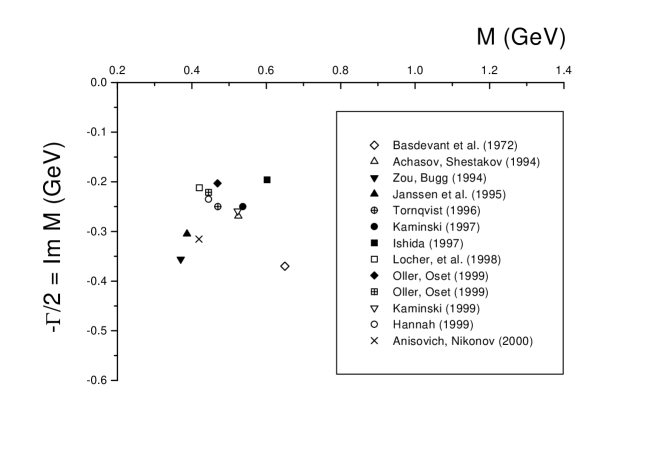
Figure 1: The poles of the $S$-matrix in the complex mass plane (GeV) corresponding to the lightest scalar resonance according to Refs.  [3] – [18].

However, owing to the strong interaction nature, it is difficult to discuss the dynamics in the $IJ=00$ channel without heavily relying on different models and approximations. These models or approximations often violate some fundamental principles. For example, in most applications of the $K$ matrix approach the dynamical effects of the left–hand cut ($l.h.c.$) are approximated by background polynomials which are beyond control theoretically. Strictly speaking, such an approximation violates crossing symmetry. It is not always clear how these assumptions and approximations influence the conclusion at quantitative or even qualitative level. Therefore it is very important to study the problem from different angles and to reduce the model dependence as much as possible.

The goal of this paper is to elucidate the role of the left–hand singularities in the determination of the position of the $\sigma$ meson. Our philosophy in this paper is to start strictly from first principles and to reduce model dependence as much as possible. Throughout the text the main assumptions we use are analyticity and single channel unitarity. We will also make use of chiral perturbation theory to estimate the left–hand cut contributions to $\pi\pi$ scattering processes in the phenomenological application. Chiral perturbation theory encounters problems at high energies, an unitarized chiral approach in studying the $\pi\pi$ system or even the $\pi\pi,\bar{K}K$ coupled–channel system has been proposed and discussed in recent years with remarkable success (see Ref. [20]–[24], and also Ref. [17]). However, our treatment of chiral perturbation theory is rather different from the standard applications based on it. Essentially we only need its prediction on cuts. We are convinced, by analyzing the $IJ=00,20$ and $11$ channels simultaneously, that chiral perturbation theory can be used reliably to elucidate the role of the $l.h.c.$ in the determination of the $\sigma$ resonance.

This paper is organized as follows: In the begining we will establish a new representation for a hadron form factor in the single–channel case. We prefer to introduce it firstly in the more traditional scattering theory in sec. 2, which may benefit some readers. The analytic structure of the $\pi$ hadronic form factor and of the $\pi\pi$ scattering $S$ matrix in the context of field theory is analyzed in the new scheme in sec. 3. Left–hand cut effects of the $\pi\pi$ scattering amplitudes are estimated in sec. 4. The sec. 5 is devoted to study the pole position of the $\sigma$ resonance. The analysis in the $IJ=20$ and $11$ channel is also made. The sec. 6 is for the conclusion.

2 The dispersion relation for a scalar form factor

2.1 Basic formulas

In this section we consider the relationship between an $S$-matrix and a scalar form factor in a single–channel scattering problem. For the benefit of the reader, we begin with a brief summary of well known properties of the scattering matrix. The $S$-matrix is related to the partial wave amplitude (we consider the case of the S-wave scattering) by

$$S(k) = 1+2ikf(k)$$ (1)

where $k$ is the channel momentum. The one–channel unitarity of the $S$ matrix in the physical region $k\geq 0$ has the form

$$S(k)^{*} = S(k)^{-1}\quad,$$ (2)

$$\mbox{Im}\;f(k) = k|f(k)|^{2}\quad.$$ (3)

The reflection property of the $S$-matrix (see e.g. [25]) leads to the following relation between positive and negative channel momenta $k$:

$$S(-k) = S^{*}(k)$$ (4)

where the connection between $k<0$ and $k>0$ is via an analytical continuation in the upper half plane. The Riemann surfaces of the $S$-matrix and the scattering amplitude as functions of energy $E=k^{2}$ have two sheets:

$$S(k) = \left\{\begin{array}[]{lcl}S_{I}(E)=1+2ik_{I}(E)f_{I}(E)&,&\mbox{Im}\;k\geq 0\\ S_{II}(E)=1+2ik_{II}(E)f_{II}(E)&,&\mbox{Im}\;k<0\end{array}\right.$$ (7)

Here $f(E)$ is the scattering amplitude, the subscript $I$ or $II$ denotes its value on the sheet I or II, and $k_{I}(E)=-k_{II}(E)$. In the following, however, we often drop the subscript (or superscript) $I$ when it causes no confusion. The reflection property (4) together with the unitarity relation (2) gives the following relations between the different branches of $S(E)$ and $f(E)$

$$S_{II}(E) = S_{I}^{*}(E)=\frac{1}{S_{I}(E)}$$ (8)

$$f_{II}(E) = \frac{f_{I}(E)}{S_{I}(E)}$$ (9)

which extend by an analytical continuation from the physical region $E\geq 0$ to the corresponding domains of analyticity on the sheets I and II.

We define the scalar form factor $A(k)$ as an analytical function of $k$ which satisfies the following unitarity relation (compare with Eq.(3))

$$\mbox{Im}\;A(k) = kA(k)f(k)^{*}\quad,\quad k\geq 0$$ (10)

and has no singularities, except for possible bound states, in any finite part of the upper half plane $\mbox{Im}\;k>0$ (that is the sheet I as the function of energy $E$). To define the scalar form factor uniquely additional constraints are needed. One is a trivial normalization condition $A(k_{0})=A_{0}$ with some choice of $k_{0}$ and $A_{0}$ convenient for physical applications.

Equation (10) has the well known Omnes–Muskhelishvili (OM) [26] solution which determines the form factor $A_{I}(E)$ on the sheet I

$$A_{I}(E) = P(E)\exp{\left(\frac{E}{\pi}\int_{0}^{\infty}\frac{\delta(E^{\prime})}{E^{\prime}(E^{\prime}-E)}dE^{\prime}\right)}$$ (11)

where $\delta(E)$ is the scattering phase:

$$S_{I}(E) = e^{2i\delta(E)}\quad,\quad E\geq 0$$ (12)

and $P(E)$ is an arbitrary real polynomial ($P(E)$ is real for real $E$). Here an once-subtraction form of the OM solution is used, and the normalization condition is absorbed in the polynomial $P(E)$.

It is useful to remember that in potential scattering the $S$-matrix and the form factor can be conveniently defined in terms of the Jost function $\mbox{${\cal F}$}(k)$ [25]

$$S(k) = \frac{\mbox{${\cal F}$}(-k)}{\mbox{${\cal F}$}(k)}$$ (13)

$$A(k) = \frac{1}{\mbox{${\cal F}$}(k)}$$ (14)

where $\mbox{${\cal F}$}(k)$ is analytical in the upper half plane ($\mbox{Im}\;k>0$) and has the reflection property:

$$\mbox{${\cal F}$}(-k) = \mbox{${\cal F}$}^{*}(k^{*})$$ (15)

In this case the polynomial $P(E)$ is reduced to a constant. Also one gets the relation between the values of the scalar form factor on the sheets I and II:

$$A_{II}(E) = \frac{A_{I}(E)}{S_{I}(E)}$$ (16)

2.2 A new representation of the scalar form factor

In this section we derive another useful representation of the scalar form factor which, to the best of our knowledge, was not described in the literature. The starting point is the unitarity condition (10) which is written in the form

$$\mbox{Im}\;A_{I}(E)=\frac{A_{I}(E+i\epsilon)-A_{I}(E-i\epsilon)}{2i} = k_{I}(E)A_{I}(E)f_{II}(E)$$ (17)

for $E\geq 0$. Here the identity $f_{I}^{*}(E)=f_{II}(E)$ for real $E$ is used. Since the scalar form factor $A_{I}(E)$ is analytical on the sheet I except for the poles corresponding to bound states at $E<0$ and the kinematical cut along the real $E$ axis, the following once–subtracted dispersion relation can be used:

$$A_{I}(E)-A_{I}(\Lambda) = \sum_{b}\frac{(\Lambda-E)\beta_{b}}{(E-E_{b})(\Lambda-E_{b})}+I(E)\ ,$$ (18)

$$I(E) = \frac{(E-\Lambda)}{2\pi i}\int_{0}^{\infty}\frac{A_{I}(z+i\epsilon)-A_{I}(z-i\epsilon)}{(z-E)(z-\Lambda)}dz$$ (19)

$$= \frac{(E-\Lambda)}{2\pi}\int_{C_{R}}\frac{k_{I}(z)A_{I}(z)f_{II}(z)}{(z-E)(z-\Lambda)}dz$$

where the sum is taken over all bound states with energies $E_{b}$, $\beta_{b}$ are the corresponding residues of the form factor in the poles on the Sheet I, $\Lambda$ is a subtraction point, and the contour $C_{R}$ envelopes the kinematical cut $0\leq E<\infty$ as shown in Fig.2.

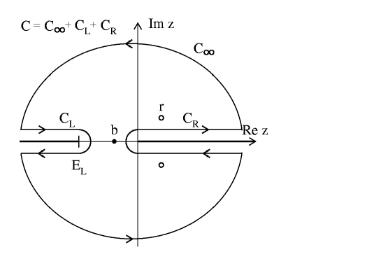
Figure 2: The integration contours used in the dispersion relations for the scalar form factor.

The integration contour can be deformed, assuming that the integrand falls off fast enough at the infinity (that is why the subtraction is needed), in such a way that it goes around the left hand cut $-\infty<E\leq E_{c}$ corresponding to the dynamical singularities related to the scattering amplitude $f_{II}(E)$ on the sheet II (see Fig.2). In the process of deformation the contour crosses several poles of the integrand. The terms $(z-E)$ and $(z-\Lambda)$ in the denominator of Eq.(19) correspond to two such poles. The bound states, if they exist, contribute via the poles on the sheet I in the factor $A_{I}(E^{\prime})$ . The virtual and resonant states correspond to the poles on the sheet II of scattering amplitude $f_{II}(E^{\prime})$. Collecting all these terms we get

$$I(E) = i(k_{I}(E)A_{I}(E)f_{II}(E)-k_{I}(\Lambda)A_{I}(\Lambda)f_{II}(\Lambda)+B(E)+R(E))$$ (21)

$$-\frac{(E-\Lambda)}{2\pi}\int_{C_{L}}\frac{k_{I}(z)A_{I}(z)f_{II}(z)}{(z-E)(z-\Lambda)}dz\ ,$$

$$B(E) = \sum_{b}\frac{\beta_{b}k_{I}(E_{b})f_{II}(E_{b})(E-\Lambda)}{(E_{b}-E)(E_{b}-\Lambda)}\ ,$$ (22)

$$R(E) = \sum_{r}\frac{k(E_{r})A_{I}(E_{r})\mbox{Res}[f_{II}(E_{r})](E-\Lambda)}{(E_{r}-E)(E_{r}-\Lambda)}\ .$$ (23)

In above the function $B(E)$ is given by the sum over all bound states (the poles $E_{b}$ of the scattering amplitude on the sheet I), and the function $R(E)$ is given by the sum over all resonances and virtual states (the poles $E_{r}$ of the scattering amplitude on the sheet II). According to Eq.(9) the poles of $S_{I}(E)$ correspond to the zeroes of $S_{II}(E)$, therefore for all bound states $b$

$$k_{I}(E_{b})f_{II}(E_{b}) = -\frac{i}{2}\ .$$ (24)

The residues of $f_{II}(E)$ in the poles $E_{i}$ on the sheet II are calculated with Eqs.(9,16):

$$k_{I}(E_{r})A_{I}(E_{r})\mbox{Res}[f_{II}(E_{r})] = \frac{iA_{I}(E_{r})}{2S^{\prime}_{I}(E_{r})}=\frac{i\beta_{r}}{2}$$ (25)

$$\beta_{r} = \mbox{Res}A_{II}(E_{r})$$ (26)

Using Eqs.(18-26) we get the following representation of the scalar form factor:

$$A_{I}(E) = \frac{S_{I}(E)}{1+S_{I}(E)}\left(A_{I}(\Lambda)\frac{1+S_{I}(\Lambda)}{S_{I}(\Lambda)}+\sum_{i=b,r}\frac{\beta_{i}}{E-E_{i}}-\sum_{i=b,r}\frac{\beta_{i}}{\Lambda-E_{i}}\right.$$ (27)

$$\left.-\frac{(E-\Lambda)}{\pi}\int^{E_{L}}_{-\infty}\frac{\Delta(E)}{(z-E)(z-\Lambda)}dz\right)$$

where the function $\Delta(E)$ is defined on the left hand cut $-\infty<E\leq E_{L}$ (see Fig.2) by

$$\Delta(E) = \frac{k_{I}(E)A_{I}(E)(f_{II}(E+i\epsilon)-f_{II}(E-i\epsilon))}{2i}$$ (28)

$$= \frac{A_{II}(E+i\epsilon)-A_{II}(E-i\epsilon)}{2i}$$ (29)

Here we used Eq.(16) in deriving the identity (29).

The Eq.(27), though very simple, has the very attractive feature that it explicitly shows the contributions resulting from different types of dynamical singularities: the bound states, the resonances, the virtual states, and the left hand cut. The poles of the scattering amplitude contribute only to the local terms in the representation (27). The sum on the $r.h.s.$ of Eq. (27) includes the poles on both the first and the second sheets. However, the poles on the sheet II are canceled by the corresponding zeros of the S-matrix on the sheet I, so that the representation (27), which determines the scalar form factor on the sheet I, contains only the poles corresponding to the bound states.

2.3 Examples

To illustrate the above described formalism we consider a simple example of a non-relativistic scattering of a particle with mass $m$ by the Yukawa potential $V(r)=g\exp{(-\mu r)}/r$. The Jost function in the first order in the coupling constant has the form

$$\mbox{${\cal F}$}{(k)} = 1-\frac{gm}{ik}\ln{(1-\frac{2ik}{\mu})}$$ (30)

For the sake of simplicity, we neglect the higher order terms because all analytical properties of the scattering matrix and the form factor are strictly preserved in any finite order of the Jost function expansion. The S–matrix corresponding to the Jost function (30) for $g<0$ has only one pole at $k=i\kappa$: it is either a virtual state on the sheet II ($\kappa<0$) or a bound state on the sheet I ($\kappa>0$). The calculations using Eq.(27) are straightforward, and typical examples for the cases of virtual and bound states are shown in Fig. 3.

(a)                                                                       (b)

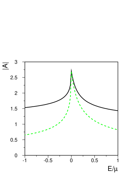
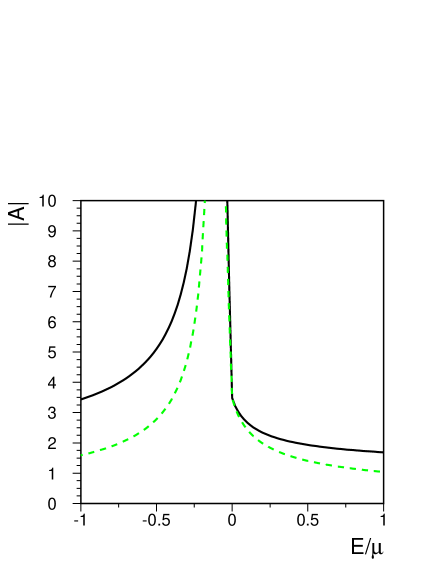
Figure 3: The scalar form factor corresponding to the Jost function defined by Eq.(30): (a) a virtual state at $k=-i0.1\mu$, (b) a bound state at $k=i0.1\mu$. The solid line is the complete result for $|A_{I}(E)|$, the dashed lines show the result in the scattering length approximation. The particle mass is set to $m=0.5$, so that $E=k^{2}$.

One commonly used approximation is to neglect explicit effects of the left hand cut and consider only a few poles of the scattering amplitude close to the physical region. In the scattering length approximation the S-matrix has the form

$$S_{a}(k) = \frac{1-ika}{1+ika}$$ (31)

where $a$ is the scattering length. In this case we have only the pole term in (27) at $2mE=k^{2}=a^{-2}$, and the subtraction term vanishes for $\Lambda\to\infty$ ($S(\infty)=-1$). This gives the well known result:

$$A_{a}(E) = \frac{A(0)}{1+ik(E)a}$$ (32)

A comparison of this result with the above considered example using $a=\pm\kappa^{-1}$ is shown in Fig. 3. The range of validity of the scattering length approximation for a weakly bound state is limited by the energy range $|E|\sim 2m/a^{2}$. Note, that the approximation Eq. (32) does not have the correct asymptotic behaviour: $A(E)\stackrel{{\scriptstyle E\to\infty}}{{\to}}1$.

Another useful example is the pole approximation for $K$ matrix. In the single–pole approximation, the $K$ matrix has the form

$$K(E) = \frac{\gamma_{1}}{E_{1}-E}$$ (33)

and the corresponding $S$ matrix is

$$S(E) = \frac{1+ik(E)K(E)}{1-ik(E)K(E)}\quad.$$ (34)

Assuming $E_{1}>0$ and $0<\gamma_{1}<2\sqrt{E_{1}}$, one finds two resonant poles at $E=E_{r}$ and $E=E_{r}^{*}$ where $E_{r}=(-i\gamma_{2}/2+\sqrt{E_{1}-\gamma_{1}^{2}/4})^{2}$. Using Eq. (27) we get

$$A_{I}(E) = \frac{S_{I}(E)}{1+S_{I}(E)}\left(\frac{a}{E-E_{r}}+\frac{a^{*}}{E-E_{r}^{*}}\right)=$$ (35)

$$= \frac{(E_{1}-E+ik_{I}(E)\gamma_{1})}{2(E_{1}-E)}\frac{C(E-E_{z})}{(E-E_{r})(E-E_{r}^{*})}$$ (36)

where $a$ is the residue of the form factor at $E=E_{r}$ and $C$ is a normalization constant. At $\gamma_{1}\neq 0$, the form factor has no pole at the bare pole position $E=E_{1}$, therefore $E_{z}=E_{1}$, and the form factor is given by

$$A_{I}(E) = \frac{(E_{1}-E+ik_{I}(E)\gamma_{1})E_{1}}{(E-E_{r})(E-E_{r}^{*})}$$ (37)

where we set $C=2E_{1}$. The $r.h.s.$ of (37) has no poles on the first energy sheet because the nominator $(E_{1}-E+ik_{I}(E)\gamma_{1})=(E_{1}-E-ik_{II}(E)\gamma_{1})$ vanishes at $E=E_{r},E_{r}^{*}$. It is easy to verify that the result (37) is equivalent the standard one pole approximation [27]:

$$A_{I}(E) = \frac{E_{1}}{(E_{1}-E-ik_{I}(E)\gamma_{1})}$$ (38)

This result can be easily generalized to the case when $K$ matrix has more than one pole.

3 The analytic form factor and the $S$ matrix in the complex $s$ plane

In the previous section we have introduced the new representation for the form factor in the complex k–plane in the language of scattering theory. It is of course straightforward to re-express all the results in the above section in relativistic quantum field theory, in the complex $s$ plane (here $s$ denotes the center of mass energy squared). Hence the spectral representation of the form factor can be written down using the well known LSZ reduction formalism,

$${\rm Im}A=A\rho T^{*}\ ,$$ (39)

where $\rho$ denotes the kinematic phase-space factor. Taking $\pi\pi$ scattering for example,

$$\rho=\sqrt{1-4m_{\pi}^{2}/s}\ .$$ (40)

In Eq. (39) $T$ denotes the scattering T matrix which satisfies the optical theorem,

$${\rm Im}T=T\rho T^{*}\ ,$$ (41)

for the physical value of $s$. Discussions parallel to that in section 2.2 can be made and Eq. (27) can be recasted as,

$$A_{I}(s) = {\frac{S_{I}}{1+S_{I}}}\{\sum_{i}{\frac{A_{I}(z_{i})}{(s-z_{i})S_{I}^{\prime}(z_{i})}}+\sum_{j}{\frac{\beta_{j}}{s-s_{j}}}+P_{n}(s)$$ (42)

$$+{\frac{1}{2\pi i}}\int_{L}{\frac{A_{I}(s^{\prime})disc\left[{\frac{1+S_{I}(s^{\prime})}{S_{I}(s^{\prime})}}\right]}{s^{\prime}-s}}ds^{\prime}\ \}\ ,$$

where the position of zeros of $S_{I}$ on the complex $s$ plane are denoted as $z_{i}$, and $s_{j}$ are the position of bound state poles of $S_{I}$ (and $A$). The $P_{n}(s)$ is a (n-1)th order real polynomial when $A(s)$ obeys a n-th subtracted dispersion relation. The discontinuity of $S$ on the $l.h.c.$ $L=(-\infty,0]$ manifests itself in the left–hand integral on the $r.h.s.$ of the above equation, even though $A$ itself does not contain left–hand singularities. Possible (n-th) subtractions on the integral in Eq.(42) are understood.

The Eq. (42) offers a convenient and powerful expression for studying the analytic structure of the scattering $S$ matrix and form factors. For example, it sets up a relation between the form factor in the time-like region and in the space-like region, provided that the $S$ matrix is known. However, we will leave it aside (except for the analysis made under some simple approximations discussed in sec. 2.3) and go directly to discuss the analytic property of the scattering T matrix. In fact, it is easy to understand that the T matrix itself satisfies Eq. (42) with only minor modifications. That is, unlike the form factor, $T$ also contains left–hand singularities. After some algebraic manipulation one can obtain (for the detail of the proof, see Appendix) ,

$$T(z)={S\over 1+S}\{\sum_{i}{\frac{i}{2\rho(z_{i})S^{\prime}(z_{i})(z-z_{i})}}+\sum_{j}{\frac{\beta_{j}}{z-s_{j}}}+P_{n}(z)$$

$$+{\frac{1}{2\pi i}}\int_{L}{\frac{{disc}\left[T(s^{\prime}){\frac{1+S(s^{\prime})}{S(s^{\prime})}}\right]}{s^{\prime}-z}}ds^{\prime}\}\ .$$ (43)

The relation $T_{I}(z_{i})=i/(2\rho(z_{i}))$ is used in deriving Eq. (3). If we define $F\equiv T(1+S)/S$ so the above equation can be rewritten as,

$$F(z)=\sum_{i}{\frac{i/2\rho(z_{i})}{S^{\prime}(z_{i})(z-z_{i})}}+\sum_{j}{\frac{\beta_{j}}{z-s_{j}}}+\\ P_{n}(z)+{\frac{1}{\pi}}\int_{L}{\frac{{\rm Im}F}{s^{\prime}-z}}ds^{\prime}\ \ .$$ (44)

The Eq. (44) sets up a dispersion relation for $F$ which contains no right–hand cut. We can further express the $S$ matrix in terms of F,

$$S=\sqrt{1-\rho^{2}F^{2}}+i\rho F\ .$$ (45)

Apparently $F$ is real when $z$ real and greater than $4m_{\pi}^{2}$. Actually ${\rm Re}T={\frac{F}{2}}$ in the physical region, hence $F$ is the analytic continuation of 2${\rm Re}T$ on the entire cut plane, and now it becomes obvious why in Eq. (44) there is no right–hand cut. Also we have,

$${\rm Im}_{R}T={\frac{1-\sqrt{1-(\rho F)^{2}}}{2\rho}}\ ,$$ (46)

for physical value of $s$. It is worth pointing out that Eq. (46) relates the imaginary part of a given partial–wave amplitude on the unitarity cut to the imaginary part of the same partial–wave amplitude on the $l.h.c.$, in a complicated manner. It is interesting to compare Eq. (46) with the following relation obtained using the Froissart–Gribov representation for the partial wave projection,

$${\rm Im}_{L}T^{I}_{l}(s) = {\left[1+(-1)^{I+L}\right]\over s-4m_{\pi}^{2}}\sum_{I^{\prime}}\sum_{l^{\prime}}(2l^{\prime}+1)C_{II^{\prime}}^{(st)}$$ (47)

$$\times\int_{4m_{\pi}^{2}}^{4m_{\pi}^{2}-s}dtP_{l}(1+{2t\over s-4m_{\pi}^{2}})P_{l^{\prime}}(1+{2s\over t-4m_{\pi}^{2}}){\rm Im}T^{I^{\prime}}_{l^{\prime}}(t)$$

which [28] relates the left–hand discontinuity to the right–hand discontinuity in a linear way, but all partial–waves are involved. To further analyze Eq. (45), we notice that $|\rho F(s)|\leq 1$ in the physical region, since in the physical region

$$\rho F(s)=\sin(2\delta)\ .$$ (48)

It is therefore easy to understand that at values of $s$ when $\delta=\pi/4+n\pi/2$ we have,

$${\frac{d}{ds}}(\rho F)=0\ ,$$ (49)

and

$${\frac{d^{2}}{ds^{2}}}(\rho F)\leq 0\,\,\,(\rho F=1)\ ;\,\,\,{\frac{d^{2}}{ds^{2}}}(\rho F)\geq 0\,\,\,(\rho F=-1)\ .$$ (50)

These requirements lead to additional constraint on the parameters in the expression of the $S$ matrix. Especially Eq. (49) and Eq. (50) indicate that the pole parameters and the discontinuity on the left are correlated to each other. For example, without further knowledge on the $l.h.c.$ integrals, Eq. (49) (Eq. (50)) enables us to establish a sum rule (inequalities) that the left–hand integral has to obey.

The Eq. (48) is important in the sense that it relates the experimental observable (the partial–wave phase shift) to the pole contributions and the $l.h.c.$ contributions in a simple and elegant manner. Unlike the conventional $K$ matrix approach, the pole parameters are physical and the two contributions from poles and $l.h.c.$ are additive. As we will see in the next section that we will be able to calculate the $l.h.c.$ integral in Eq. (44) in a reliable way, hence Eq. (48) offers a convenient method to fit the pole positions. It is worth emphasizing that Eqs. (44) and (48) are valid for any partial–wave amplitude hence they afford a unified approach for determining resonances in different channels. This is remarkable since the output from different channels can be compared to each other and this feature is very important to evaluate the quality of the method and approximations being used in the fit.

4 Estimates on the left–hand cut effects of $\pi\pi$ scatterings in chiral perturbation theory

In above discussions we have re-expressed the form factor and the $S$ matrix in a way that their dependence on isolated singularities and the $l.h.c.$ are explicitly exhibited. Since the effects of the unitarity cut are dissolved, the impact of the left–hand singularities on the analytic structure of the amplitude is singled out. These formulas can be particularly useful when the fine structure of the $l.h.c.$ becomes important, which has been ignored by most applications of the K–matrix approach. For example, when determining the pole position of the $\sigma$ resonance from $\pi\pi$ phase shift, since the $\sigma$ particle’s mass is rather low, one has to carefully take into account the fine structure of the $l.h.c.$, as being emphasized recently in Ref. [18, 29]. Inspired by this we in the following carefully discuss the effects of the left–hand singularities. In order to achieve this and to reduce the model dependence as much as possible we need a method to estimate the $l.h.c.$ of $\pi\pi$ scattering amplitudes in a reliable way. The chiral perturbation theory ($\chi$PT) affords us such a method. The $\chi$PT treats the $T$ matrix as a perturbative power expansion of the external momentum and works very well at low energies. Of course, a calculation in $\chi$PT to any finite order in the power expansion would not reconstruct the pole structure, therefore $\chi$PT encounter problems when there is a resonance near the physical region on the right–hand side of the complex plane. However we argue that its predictive power in the region near the $l.h.c.$ would suffer much less from such a problem since the pole position is further away from the left–hand cut. Our strategy is clear from the above discussion: We extract from the 1–loop $\chi$PT results of the T matrix [30] the term relevant to the left–hand discontinuity to estimate the left–hand integral in Eq. (44). To be precise, the 1–loop $\chi$PT results for $\pi\pi$ scatterings are,

$$T^{I=0} = 3A(s,t,u)+A(t,u,s)+A(u,s,t)\ ,$$

$$T^{I=1} = A(t,u,s)-A(u,t,s)\ ,$$

$$T^{I=2} = A(t,u,s)+A(u,t,s)$$ (51)

where

$$A(s,t,u) = {s-m_{\pi}^{2}\over f_{\pi}^{2}}+B(s,t,u)+C(s,t,u)+O(E^{6})\ ,$$

$$B(s,t,u) = {1\over 6f_{\pi}^{4}}\{3(s^{2}-m_{\pi}^{4}){\bar{J}}(s)+\left[t(t-u)-2m_{\pi}^{2}t+4m_{\pi}^{2}u-2m_{\pi}^{4}\right]{\bar{J}}(t)$$ (52)

$$+(t\leftrightarrow u)\}\ ,$$

and the function $C$ is a polynomial of $s$, $t$ and $u$ which is irrelevant here. The function ${\bar{J}}(s)$ is defined as,

$${\bar{J}}(s) = {1\over 16\pi^{2}}\left[\rho{\rm ln}\left({\rho-1\over\rho+1}\right)+2\right]\ .$$ (53)

The partial wave projection can be carried out:

$$T_{J}^{I}(s)={1\over 32\pi(s-4m_{\pi}^{2})}\int^{0}_{4m_{\pi}^{2}-s}dt\,P_{J}(1+{2t\over s-4m_{\pi}^{2}})T^{I}(s,t,u)$$ (54)

from which the discontinuity of $T$ on the left can be obtained under certain conditions [28],

$${\rm Im}_{L}{T^{I}_{J}(s)}={1+(-1)^{I+J}\over 32\pi(s-4m_{\pi}^{2})}\int_{4m_{\pi}^{2}}^{4m_{\pi}^{2}-s}dt\,P_{J}(1+{2t\over s-4m_{\pi}^{2}}){\rm Im}T^{I}_{t}(s,t)\,\,\,;s\leq 0\ .$$ (55)

However, for scattering amplitudes in chiral perturbation theory, the left–hand cut can be directly extracted from the analytic expressions of partial wave amplitudes. In the $I=J=0$ channel the result is,

$${\rm Im}_{L}T_{0}^{0}(s) = {1\over 1536\pi^{2}f_{\pi}^{4}(s-4m_{\pi}^{2})}\{2\cdot{\rm ln}{\sqrt{4m_{\pi}^{2}-s}-\sqrt{-s}\over\sqrt{4m_{\pi}^{2}-s}+\sqrt{-s}}(25m_{\pi}^{6}-6m_{\pi}^{4}s)$$ (56)

$$+\sqrt{-s(4m_{\pi}^{2}-s)}({7\over 3}s^{2}-{40\over 3}m_{\pi}^{2}s+25m_{\pi}^{4})\}\ .$$

However, this result is still not directly applicable here. Remember that the function $F$ is an analytic continuation of (2 times) Re$T$, which is the real part of $T$ defined in the physical region. Since ${\rm Im}_{R}T$ also develops a discontinuity on the left this part must be subtracted from ${\rm Im}_{L}T$. Therefore the correct expression for ${\rm Im}_{L}F$ is,

$${\rm Im}_{L}F=2({\rm Im}_{L}T-{\rm Re}_{L}{\rm Im}_{R}T)\ .$$ (57)

The 1–loop result of ${\rm Im}_{R}T_{0}^{0}$ is simply obtainable using the Born term amplitude and the optical theorem,

$${\rm Im}_{R}T_{0}^{0}=\rho\left({2s-m_{\pi}^{2}\over 32\pi f_{\pi}^{2}}\right)^{2}\ ,$$ (58)

for which we have ${\rm Re}_{L}{\rm Im}_{R}T={\rm Im}_{R}T$ since $\rho$ is real on the left. It is worth pointing out that in Eq. (57) the main contribution to ${\rm Im}_{L}F$ comes from the second term on the $r.h.s.$,  i.e., the term ${\rm Im}_{L}T$ is numerically rather small comparing with ${\rm Im}_{R}T$ evaluated on the $l.h.c.$ (For previous discussions on the smallness of ${\rm Im}_{L}T$, see for example Ref. [12].).

We also list the results in $I=J=1$ and $I=2,J=0$ channel from chiral perturbation theory:

$${\rm Im}_{L}T^{1}_{1} = {1\over 9216\pi^{2}f_{\pi}^{4}(s-4m_{\pi}^{2})^{2}}\{(36m_{\pi}^{6}-72m_{\pi}^{4}s+16m_{\pi}^{2}s^{2}-s^{3})$$ (59)

$$\times\sqrt{-s(4m_{\pi}^{2}-s)}+12m_{\pi}^{4}(6m_{\pi}^{4}+13m_{\pi}^{2}s-3s^{2})$$

$$\times{\rm ln}{\sqrt{4m_{\pi}^{2}-s}-\sqrt{-s}\over\sqrt{4m_{\pi}^{2}-s}+\sqrt{-s}}\}\ ,$$

$${\rm Im}_{R}T_{1}^{1} = \rho\left(s-4m_{\pi}^{2}\over 96\pi f_{\pi}^{2}\right)^{2}\ ;$$ (60)

$${\rm Im}_{L}T^{2}_{0} = {1\over 1536\pi^{2}f_{\pi}^{4}(s-4m_{\pi}^{2})}\{{1\over 6}(6m_{\pi}^{4}-32m_{\pi}^{2}s+11s^{2})\sqrt{-s(4m_{\pi}^{2}-s)}$$ (61)

$$+2(m_{\pi}^{6}+3m_{\pi}^{4}s)\times{\rm ln}{\sqrt{4m_{\pi}^{2}-s}-\sqrt{-s}\over\sqrt{4m_{\pi}^{2}-s}+\sqrt{-s}}\}\ ,$$

$${\rm Im}_{R}T^{2}_{0} = \rho\left({s-2m_{\pi}^{2}\over 32\pi f_{\pi}^{2}}\right)^{2}\ ,$$ (62)

where $f_{\pi}=93.3$MeV and the expressions listed above are valid up to $O(p^{4})$ term in the chiral expansion. It is worth pointing out that at $s=m_{\pi}^{2}/2$, $4m_{\pi}^{2}$ and $2m_{\pi}^{2}$ the $lowest$ $order$ partial wave amplitudes $T_{0}^{0}$, $T^{1}_{1}$ and $T^{2}_{0}$ vanish respectively, as a consequence of the Adler zero condition.

5 The determination of the $\sigma$ resonance in $\pi\pi$ scatterings

5.1 A description to the fit procedure

Having obtained the analytic expressions of ${\rm Im}_{L}F$ for the partial wave amplitudes it becomes possible to use the experimental data on $\pi\pi$ scattering phase shifts to determine the pole positions in various channels. We fit both IJ=00, 11 and 20 channels. In the following we briefly describe the procedure and the method for the fit:

1. We assume the $\pi\pi$ scattering amplitude $T$ satisfies a once subtracted dispersion relation from physical considerations. So our left–hand integral is once subtracted at $s=m_{\pi}^{2}/2$, $s=4m_{\pi}^{2}$ and $s=2m_{\pi}^{2}$ for IJ=00, 11 and 20, respectively. The positions of the subtraction points are chosen only for the convenience of discussions.

2. A dispersion integral in $\chi$PT needs many subtractions and this is artificial because of the bad high energy behavior of $\chi$PT amplitudes. So we always truncate the once subtracted integral at $-\Lambda_{\chi PT}^{2}$ where $\Lambda_{\chi PT}$ ranges from, for example, $700$MeV to $1$GeV. We argue that the influence from the region $|\sqrt{s}|\geq\Lambda_{\chi PT}$ is negligible to the physics we are concerning. We realize that the value $|s|\simeq 1$GeV is too large for chiral perturbation theory to be valid. We however take this value just for the purpose of testing to what extent our fit results depending on the behavior of ${\rm Im}_{L}F$. We have to make sure that the mass and the width of the resonance obtained under such an approximation have to be insensitive to the choice of the cutoff. To compare with perturbation results we will also extract ${\rm Im}_{L}F$ from the unitarized T matrix, i.e., the [1,1] Padé approximant, in the I=J=0 channel.

3. In the three channels IJ=00, 11 and 20, we assume one pole in the first two cases. In the IJ=11 channel the threshold behavior ($T\sim\rho^{3}$ near threshold) is considered to reduce one parameter (the subtraction constant). In our fit each pole contains 4 parameters. Two of them are related to the position of the pole. The other two are related to the couplings of the pole to $F$. That is the coefficient $\alpha_{i}\equiv i/(2\rho(z_{i})S^{\prime}(z_{i}))$ in Eq. (44). One may relate $\alpha_{i}$ to $z_{i}$ in the narrow resonance approximation or in models. But for the wide resonance $\sigma$ there is no simple relation between the two, so we take $\alpha_{i}$ as completely free as an approximation. However, we also fit in the I=J=1 channel by treating ${\rm Re}\alpha_{i}$ and/or ${\rm Im}\alpha_{i}$ as the one obtained from the narrow width approximation.

5.2 Numerical results and discussions

The numerical results of the fit in the IJ=11 and 20 channels are presented below:

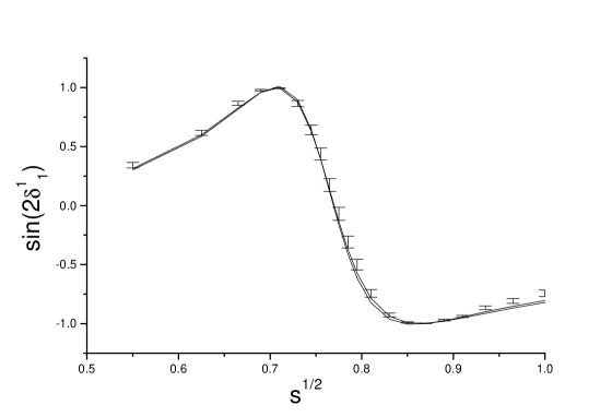
Figure 4: The fit in the I=J=1 channel with and without $l.h.c.$ effects.

1. The I=J=1 channel: The data are taken from table VI of Ref. [31]. We find that the $l.h.c.$ effect is very small in this channel. When taking $\alpha_{\rho}$ for free (so it is a 4 parameter fit) we obtain $M_{\rho}=753$MeV, $\Gamma_{\rho}=142$MeV for $\Lambda_{\chi PT}=1.0$GeV. Without $l.h.c.$ while taking $\alpha_{\rho}$ for free, we have instead $M_{\rho}=756$MeV, $\Gamma_{\rho}=144$MeV (See Fig. 4 for the fit). We also tried to fix ${\rm Re}\alpha_{i}$ and/or ${\rm Im}\alpha_{i}$ using the narrow resonance approximation. The pole position obtained using different approaches agree with each other within a few MeV. The $\chi^{2}$ is sensitive to different approaches, but the pole position is not.

2. The I=2, J=0 channel:

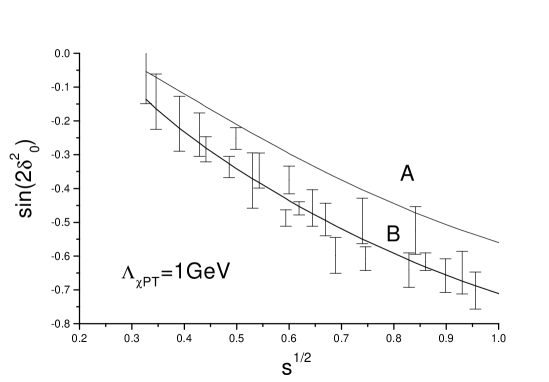
Figure 5: Contributions to the scattering phase from the left–hand integral (once subtraction at $s=2m_{\pi}^{2}$ is used) in the $I=2,J=0$ channel. Line A corresponds to setting $T^{2}_{0}(s=2m_{\pi}^{2})=0$ and be parameter free. and line B corresponds to a free subtraction constant fixed by minimizing $\chi^{2}$. The data are from Ref. [32].

   Since there is no resonance pole in this channel it is a one parameter (the subtraction constant) fit here when $\Lambda_{\chi PT}$ is held fixed. We notice that the I=2, J=0 channel favors a large value of $\Lambda_{\chi PT}$. As we see from the line B of Fig. 5 the phase shift is reproduced ideally by the $l.h.c.$ integral plus one subtraction constant. The scattering length is estimated to be $a_{0}^{2}=-0.052$ which is about 2$\sigma$ away from the experimental value, $a_{0}^{2}(exp)=-0.028\pm 0.012$  and the most recent value from the E865 Collaboration [35]: $a_{0}^{2}(exp)=-0.036\pm 0.009$ The case without the subtraction constant is also depicted in Fig. 5 as line A. The latter is equivalent to imposing the Adler zero condition for the I=2, J=0 partial–wave amplitude, since in here the dispersion integral is subtracted at $s=2m_{\pi}^{2}$. The scattering length $a_{0}^{2}=-0.032$ for the latter case, which is within 1$\sigma$ error bar comparing with the experimental value. See also footnote 2 for further information.

In the I=J=1 channel the $\rho$ resonance almost saturates the experimental phase shift and hence it demonstrates that the contribution from the left–hand integral must be very small, and it is correctly predicted by chiral perturbation theory. In contrast, no resonance exists in the I=2, J=0 channel. It is of course very satisfiable to see that the contribution from the left–hand integral to $\delta_{0}^{2}$ is in the right direction, and combining the contribution from the subtraction constant it can saturate the phase shift.

From the above discussions we see that $\chi PT$ gives satisfactory results in both the IJ=11 and 20 channel. We may obtain an impression from the above discussion that the chiral prediction works well at least in qualitative sense, i.e., the order of magnitude and the sign of the left hand integrals. In the following we turn to discuss the more interesting case of the I=J=0 channel.

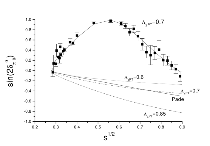
Figure 6: A typical fit of 5 parameters (4 resonance + 1 subtraction constant) in the I=J=0 channel, with $\Lambda_{\chi PT}$=0.7GeV and the experimental constraint on $a_{0}^{0}$. Different estimates on the left–hand integral are also plotted: The dotted line corresponds to $\Lambda_{\chi PT}=0.6GeV$, the dashed line corresponds to $\Lambda_{\chi PT}=0.7GeV$, the dot–dashed line corresponds to $\Lambda_{\chi PT}=0.85GeV$ and the solid line corresponds to the Padé solution.

In an earlier version of the present paper, we take the data the same as that in Ref. [7], that is the CERN-Munich data [32, 33] combining with the data from $K_{e4}$ decay near threshold [34] obtained more than 20 years ago. The most recent experiment on $K_{e4}$ decay performed by the E865 Collaboration [35] is remarkable. It affords high statistic data on the $\pi\pi$ scattering phase shifts near threshold from which the scattering length parameter $a_{0}^{0}$ can be determined with much improved accuracy: $a_{0}^{0}=0.228\pm 0.012\pm 0.003$. We therefore incorporate the new experimental results in our fit below. Here we truncate the CERN-Munich data at 900 MeV in an attempt to reduce the pollution from the $f_{0}(980)$ resonance. Since the latter (or more cautiously, its second sheet pole) is only a narrow resonance, its influence should not be very important to the determination of the $\sigma$ resonance. As we see from table 1 the pole position is not very sensitive to $\Lambda_{\chi PT}$. Including the $l.h.c.$ contribution does reduce the mass and width of the $\sigma$ particle, but the effect is not dramatic. The $\chi^{2}$ are good for all cases, see Fig. 6 for the fit.

	$M_{\sigma}$	$\Gamma_{\sigma}$
$\Lambda_{\chi PT}=1000$	477	564
$\Lambda_{\chi PT}=850$	503	587
$\Lambda_{\chi PT}=700$	519	605
Padé	519	579
no $l.h.c.$	544	607

Table 1: The pole position of the $\sigma$ resonance obtained by a fit of the data from Refs. [32, 33, 34] and [35]. The scattering length $a_{0}^{0}$ obtained in the global fit ranges from $0.25\sim 0.26$. The data in the table are in units of MeV.

It is very impressive to notice that in the I=J=0 channel the contribution from the left–hand integral to $\sin(2\delta_{0}^{0})$ has the wrong sign comparing with the experimental value. To clearly show this we draw in Fig. 6 the contribution from the left–hand integral alone to $\sin(2\delta_{0}^{0})$ in several cases, the curves are always negative and concave regardless of the different choice of cutoff parameters.  The procedure presented above clearly demonstrates the existence of the $\sigma$ meson, in a model independent way  since within our scheme the ‘background phase’ or the cut becomes calculable, from the principle of maximal analyticity no other contribution except the $\sigma$ pole can be introduced to fit the experimental data. The subtraction constant, which represents the contribution from high energies, can not generate the convex curvature that the experimental value of $\sin(2\delta_{\pi})$ exhibits.

A cautious reader may worry about the convergence problem of the chiral expansion in the large $\Lambda_{\chi PT}$ region, even though the qualitative behavior of the left hand integrals obtained from perturbation theory can be examined by varying the cutoff parameter. To overcome the difficulty we also estimated ${\rm Im}_{L}F$ in a ‘unitarized approach’, though crossing symmetry is no longer maintained in such an approximation. That is we use the [1,1] Padé approximation to obtain the unitarized scattering amplitude (in which the standard values of the $L_{i}$ parameters of the Gasser–Leutwyler Lagrangian are used) and extract the quantity ${\rm Im}_{L}F$ on the left, and insert the obtained ${\rm Im}_{L}F$ into Eq. (44). The left hand integral evaluated from the unitarized amplitude is also plotted in Fig. 6 and we find that no major conclusion is changed. It is worth pointing out that such a use of the Padé approximation is different from the standard usage of unitarization (see for example Ref. [20]–[24]). Essentially we only need the information of the unitarized amplitude on the cuts evaluated on the left, and the two approaches are not technically equivalent.

However, the scattering length parameter $a_{0}^{0}$ obtained in the global fit given in table 1 ranges from $0.25\sim 0.26$, which is about (or more than) 2$\sigma$ away from the newly obtained experimental result (It may be worth noticing that without the new $K_{e4}$ data the $a_{0}^{0}$ parameter obtained in our procedure would be much larger, $a_{0}^{0}=0.35\sim 0.37$.). To remedy this we also include in our fit program by brute force the experimental constraint $a_{0}^{0}=0.228\pm 0.012\pm 0.003$. The results are given in table 2. The fit result for $a_{0}^{0}$, ranging from $0.230\sim 0.231$, is stable against different treatment of the left–hand integrals.

	$M_{\sigma}$	$\Gamma_{\sigma}$
$\Lambda_{\chi PT}=1000$	454	648
$\Lambda_{\chi PT}=850$	479	658
$\Lambda_{\chi PT}=700$	500	662
Padé	498	642
no $l.h.c.$	525	654

Table 2: The pole position of the $\sigma$ resonance with the new experimental constraint on $a_{0}^{0}$. The value of $a_{0}^{0}$ in the global fit ranges from $0.230\sim 0.231$.

By comparing table 1 with table 2 we find that the pole position of the $\sigma$ resonance is sensitive to the scattering length parameter, but the influence is not as dramatic as in the case without the new $K_{e4}$ data from the E865 Collaboration: the pole position would be much more sensitive to the scattering length parameter in the latter case.

In discussions above we limit ourselves to a single channel analysis, therefore the possible influence from higher resonances, especially the $f_{0}(980)$, is omitted. We point out here that within the single channel approximation the influence of the $f_{0}(980)$ resonance to the fit can also be estimated (to be exact, in a model dependent way) using the method of Ref. [37], by subtracting the phase contributed from $f_{0}(980)$ alone. The mass and the width of the $\sigma$ particle change only slightly when $f_{0}(980)$ is taken into account, but the qualitative role of the $l.h.c.$ is still unchanged, that is it has only a mild influence.

As we can see from tables 1 and 2 that the pole position of the $\sigma$ resonance on the complex $s$ plane, $s_{\sigma}$, moves towards left once the value of $a_{0}^{0}$ is decreased . The phenomenon that the real part of the pole position of the $\sigma$ resonance is small has been noticed and investigated by Anisovich and Nikonov [18]. An interesting mechanism was proposed to explain this phenomenon by suggesting a strong singularity associated with the $l.h.c.$, which is simulated by a series of poles on the negative real axis fixed by the N/D equation and the experimental data. Our calculation confirms that the inclusion of the $l.h.c.$ effect pushes the $\sigma$ pole towards left but the effect is mild, and Re[$s_{\sigma}$] is also found to be sensitive to the value of the scattering length parameter. The difference between our treatment on the $l.h.c.$ and that of Anisovich and Nikonov is that the left–hand singularity of the T matrix in our case comes solely from the absorptive singularity, $i.e.$, the 2$\pi$ cuts in crossed channels. Due to relativistic kinematics, the quantity $F$ contains an additional contribution from the $s$ channel absorptive singularity, which is also from the $2\pi$ cut.  It may be illuminating to quote from Ref. [39], “There are $no$ such singularities which are associated with the quark–gluon structure of hadrons, since there are no absorptive thresholds related to this structure”.

6 Conclusion

The method proposed in this paper to discuss $\pi\pi$ interactions is based on a dispersion relation set up for the analytic continuation of the real part of the scattering T matrix. The main formula Eq. (44), though very simple, is shown to be very useful in clarifying different contributions from poles or the left–hand cut to the scattering phase shift. The procedure in deriving Eq. (44) fully respects analyticity, unitarity and crossing symmetry.

Our estimate on the left–hand cut of the scattering T matrix obeys the standard rule of $S$ matrix theory, that is the left–hand singularity comes solely from physical absorptive singularities in the crossed channel. In here they are the 2$\pi$ cuts from $t$ and $u$ channels. For the quantity $F$, it also contains the part originated from the $s$ channel absorptive singularity, as an effect of the relativistic kinematics.

We have carefully examined the reliability in using chiral perturbation theory to estimate the left–hand cut effects in various channels. Chiral perturbation theory encounters the problem of a bad high energy behavior, especially in the I=J=0 channel. This drawback was partially corrected by using a ‘unitarized approach’ to the perturbation series. It is remarkable to notice that the $l.h.c.$ contribution to $\sin(2\delta^{0}_{0})$ is negative and concave which clearly demonstrates the existence of the $\sigma$ resonance, according to the principle of maximal analyticity.

We have shown that the left–hand cut effects are mild in determining the pole position of the $\sigma$ resonance, and the effect of the scattering length in the determination of the $\sigma$ pole position is also clarified. The estimated central value of the mass and the width of the $\sigma$ meson are found to be 498 MeV and 642 MeV, respectively, if we are allowed to quote from the Padé solution with the experimental constraint on $a_{0}^{0}$. The new experimental data from the E865 Collaboration on $K_{e4}$ decay is found to be crucial in minimizing the uncertainty caused by $a_{0}^{0}$ in the determination of the $\sigma$ pole position within our scheme.

The current procedure can be extended to discuss the more general case of coupled–channel system where the $f_{0}(980)$ resonance has to be taken into account [40]. No major conclusion on the pole position of the $\sigma$ resonance and the role of the left–hand cut and the scattering length parameter is changed.

${\bf Acknowledgement}$: We would like to thank Milan Locher, Chuan-Rong Wang, Bingsong Zou for valuable discussions. Especially we are in debt to Valeri Markushin for his long and patient discussions, part of sec. 2 is written by him. We also thank Qin Ang for his assistance in performing the Padé approximation. The work of H. Z. is supported in part by National Natural Science Foundation of China under grant No. 19775005.

Appendix A Appendix

By definition

$$S=1+2i\rho T$$ (63)

and from unitarity relation

$${\rm Im}T=T\rho T^{*}\ ,$$ (64)

We can get the analytic continuation of T on the second sheet by using the reflection property,

$$T^{I}(s+i\epsilon)-T^{II}(s+i\epsilon)=2i\rho(s+i\epsilon)T^{I}(s+i\epsilon)T^{II}(s+i\epsilon)\ ,$$ (65)

or more concisely,

$$T^{II}={T^{I}\over 1+2i\rho T^{I}}={T^{I}\over S^{I}}\ .$$ (66)

Suppose the integration over the infinite circle is zero and using Cauchy’s theorem we get

$$T(s) = {1\over 2\pi i}\int_{C_{R}}{T(s^{\prime})\over s^{\prime}-s}ds^{\prime}+{1\over 2\pi i}\int_{C_{L}}{T(s^{\prime})\over s^{\prime}-s}ds^{\prime}+\sum_{j}{\beta_{j}\over s-s_{j}}$$ (67)

$$= {1\over\pi}\int_{4m_{\pi}^{2}}^{\infty}{{\rm Im}T(s^{\prime})\over s^{\prime}-s}ds^{\prime}+{1\over 2\pi i}\int_{-\infty}^{0}{discT(s^{\prime})\over s^{\prime}-s}ds^{\prime}+\sum_{j}{\beta_{j}\over s-s_{j}}$$

$$= {1\over\pi}\int_{4m_{\pi}^{2}}^{\infty}{\rho(s^{\prime})T(s^{\prime})T^{*}(s^{\prime})\over s^{\prime}-s}ds^{\prime}+{1\over 2\pi i}\int_{-\infty}^{0}{discT(s^{\prime})\over s^{\prime}-s}ds^{\prime}+\sum_{j}{\beta_{j}\over s-s_{j}}\ .$$

On the $r.h.s.$ we have

$$\rho(s)T^{I}(s)T^{I*}(s) = \rho(s+i\epsilon)T^{I}(s+i\epsilon)T^{II}(s+i\epsilon),$$ (68)

$$= -\rho(s-i\epsilon)T^{II}(s-i\epsilon)T^{I}(s-i\epsilon)\ ,$$

therefore we have

$$T(s) = {1\over 2\pi}\int_{C_{R}}{\rho(s^{\prime})T(s^{\prime})T^{II}(s^{\prime})\over s^{\prime}-s}ds^{\prime}+{1\over 2\pi i}\int_{-\infty}^{0}{discT(s^{\prime})\over s^{\prime}-s}ds^{\prime}+\sum_{j}{\beta_{j}\over s-s_{j}}$$ (69)

$$= {1\over 2\pi}\int_{C}{\rho(s^{\prime})T(s^{\prime})T^{II}(s^{\prime})\over s^{\prime}-s}ds^{\prime}-{1\over 2\pi}\int_{C_{L}}{\rho(s^{\prime})T(s^{\prime})T^{II}(s^{\prime})\over s^{\prime}-s}ds^{\prime}$$

$$+{1\over 2\pi i}\int_{-\infty}^{0}{discT(s^{\prime})\over s^{\prime}-s}ds^{\prime}+\sum_{j}{\beta_{j}\over s-s_{j}}$$

$$= {1\over 2\pi i}\int_{C}{T(s^{\prime})({S^{I}-1\over 2S^{I}})\over s^{\prime}-s}ds^{\prime}+{1\over 2\pi i}\int_{-\infty}^{0}{disc(T(s^{\prime}){S^{I}+1\over 2S^{I}})\over s^{\prime}-s}ds^{\prime}+\sum_{j}{\beta_{j}\over s-s_{j}}$$

$$= \Phi+{1\over 2\pi i}\int_{-\infty}^{0}{disc(T(s^{\prime}){S^{I}+1\over 2S^{I}})\over s^{\prime}-s}ds^{\prime}+\sum_{j}{\beta_{j}\over s-s_{j}}$$ (70)

where

$$\Phi \equiv {1\over{2\pi i}}\int_{C}{T(s^{\prime})({S^{I}-1\over 2S^{I}})\over s^{\prime}-s}ds^{\prime}$$ (71)

$$= T({S^{I}-1\over 2S^{I}})+\sum_{i}{1/2i\rho(s_{i})\over{2S^{I}(s_{i})}^{\prime}(s_{i}-s)}-\sum_{j}{\beta_{j}\over 2(s-s_{j})}\ .$$

In the derivation of Eq. (69), by combining the second and the third term on the right hand side of the second equation of (69) and using

$$\rho T^{II}={S^{I}-1\over 2iS^{I}}$$ (72)

we get the third equation of (69). And by substituting $\Phi$ into (69) we obtain

$$T(s)={S\over S+1}\left[\sum_{i}{i\over 2\rho(s_{i}){S(s_{i})}^{\prime}(s-s_{i})}+\sum_{j}{\beta_{j}\over s-s_{j}}+{1\over 2\pi i}\int_{-\infty}^{0}{disc(T(s^{\prime}){S+1\over S})\over s^{\prime}-s}ds^{\prime}\right]\ .$$ (73)

References

- [1] Review of Particle Physics, Eur. Phys. J. C15 (2000) 1.
- [2] Review of Particle Physics, Eur. Phys. J. C3 (1998) 1.
- [3] J. L. Basdevant, C. D. Froggatt, J. L. Petersen, Phys. Lett. B41 (1972) 178.
- [4] N.N. Achasov, G.N. Shestakov, Phys. Rev. D 49, 5779 (1994).
- [5] R. Kamiński, L. Leśniak, and J.-P. Maillet, Phys. Rev. D 50, 3145 (1994).
- [6] R. Kamiński ., Phys. Lett. B413, 130 (1997)
- [7] B. S. Zou and D. V. Bugg, Phys. Rev. D 48, R3948 (1994); Phys. Rev. D 50, 591 (1994).
- [8] G. Janssen, B.C. Pearce, K. Holinde, and J. Speth, Phys. Rev. D. 52, 2690 (1995).
- [9] N. A. Törnqvist, Z. Phys. C 68, 647 (1995).
- [10] N. A. Törnqvist and M. Roos, Phys. Rev. Lett. 76, 1575 (1996).
- [11] J. A. Oller and E. Oset, Nucl. Phys. A620, 438 (1997).
- [12] J. A. Oller and E. Oset, Phys. Rev. D60, 074023 (1999).
- [13] J. A. Oller , Phys. Rev. D60, (1999) 099906.
- [14] R. Kamiński, L. Leśniak, and B. Loiseau, Eur. Phys. J. C 9, 141 (1999).
- [15] S. Ishida et al., Prog. Theor. Phys. 98 (1997) 1005.
- [16] M. P. Locher, V. E. Markushin, H. Q. Zheng, Eur. Phys. J. C 4, 317 (1998).
- [17] T. Hannah, Phys. Rev. D 60 017502 (1999).
- [18] V. V. Anisovich, V. A. Nikonov, Eur. Phys. J. A8 (2000) 401; V. V. Anisovich and V. A. Nikonov, hep-ph/9911512.
- [19] N. A. Tornqvist, Invited talk at YITP Workshop on Possible Existence of the sigma meson and it Implications to Hadron Physics, Kyoto, Japan, 12-14 Jun 2000, hep-ph/0008135; N.A. Tornqvist and A.D. Polosa, hep-ph/0011109; Yu.S. Surovtsev, D. Krupa and M. Nagy, Talk given at Meson 2000 Workshop, Cracow, Poland, 19-23 May 2000, hep-ph/0009039; S. Narison, Talk given at YITP Workshop on Possible Existence of the sigma meson and it Implications to Hadron Physics (sigma-meson 2000), Kyoto, Japan, 12-14 Jun 2000 and at the International EuroConference in Quantum Chromodynamics: 15 Years of the QCD - Montpellier Conference (QCD 00), Montpellier, France, 6-13 Jul 2000, hep-ph/0009108; M. Harada, Talk given at YITP Workshop on Possible Existence of the sigma meson and it Implications to Hadron Physics (sigma-meson 2000), Kyoto, Japan, 12-14 Jun 2000, hep-ph/0009051; J. A. Oller, Talk at YITP Workshop on Possible Existence of the sigma meson and it Implications to Hadron Physics (sigma-meson 2000), Kyoto, Japan, 12-14 Jun 2000, hep-ph/0007349; P. Minkowski, Nucl. Phys. Proc. Suppl. 86, 372 (2000); R. Kaminski, L. Lesniak and B. Loiseau, Presented at Meson 2000 Workshop, Cracow, Poland, 19-23 May 2000, hep-ph/0006303; M. Ishida, Talk at YITP Workshop on Possible Existence of the sigma meson and it Implications to Hadron Physics (sigma-meson 2000), Kyoto, Japan, 12-14 Jun 2000, hep-ph/0012325.
- [20] T. N. Truong, Phys. Rev. Lett. 61 (1988)2526.
- [21] A. Dobado and J. R. Pelaez, Phys. Rev. D56 (1997) 3057.
- [22] J. A. Oller, E. Oset and J. R. Pelaez, Phys. Rev. Lett. 80 (1998) 3452; Phys. Rev. D 59 (1999) 074001.
- [23] F. Guerrero and J. A. Oller, Nucl. Phys. B537 (1999) 459.
- [24] J. A. Oller, E. Oset and A. Ramos, Prog. Part. Nucl. Phys. 45 (2000) 157.
- [25] R. G. Newton, Scattering theory of waves and particles, 2nd ed., Springer–Verlag publishers, 1982, New York.
- [26] N. I. Muskhelishvili, Singular Integral Equations, (Moscow, 1946); R. Omnès, Nuovo Cimento 8, 316 (1958).
- [27] G. Barton, , W. A. Benjamin INC, New York 1965.
- [28] B. R. Martin, D. Morgan and G. Shaw, – , Academic press, 1976, London.
- [29] V. E. Markushin and M. P. Locher, Talk given at the workshop on Hadron Spectroscopy, Frascati, March 8–12, 1999. Preprint PSI-PR-99-15.
- [30] J. Gasser and H. Leutwyler, Ann. of Phys. 158 (1984)142; J. Gasser and U. Meisner, Nucl. Phys. B357 (1991) 90, and referrences therein.
- [31] S. D. Protopopescu et al., Phys. Rev. D7 (1973) 1279.
- [32] G. Grayer et al., Nucl. Phys. B75 (1974) 189; W. Ochs, Ph.D. thesis, Munich Univ., 1974.
- [33] W. Maenner, in – 1974 (Boston), Proceedings of the fourth International Conference on Meson Spectroscopy, edited by D. A. Garelick, AIP Conf. Proc. No. 21 (AIP, New York, 1974).
- [34] L. Rosselet et al., Phys. Rev. D15 (1977) 574.
- [35] P. Truol (E865 Collaboration), hep-ex/0012012.
- [36] M. Ishida et. al., Talk given at the workshop on Hadron Spectroscopy, Frascati, March 8–12, 1999; hep-ph/9905261.
- [37] M. Locher, V. Markushin and H. Q. Zheng, Phys. Rev. D55, (1997) 2894; B. S. Zou and D. V. Bugg, Phys. Rev. D50 (1994) 591.
- [38] M. Boglione and M. R. Pennington. Z. Phys. C75 (1997) 113.
- [39] R. Oehme, Int. J. Mod. Phys. A10 (1995)1995.
- [40] Z. G. Xiao and H. Q. Zheng, hep-ph/0103042.