Abstract

We construct an analytical expression for the distribution of gluons in the state immediately following a heavy ion collision in the quasi–classical limit of QCD given by McLerran–Venugopalan model. The resulting gluon number distribution function includes the effects of all multiple rescatterings of gluons with the nucleons of both colliding nuclei. The typical transverse momentum $k_{\perp}$ of the produced gluons is shown to be of the order of the saturation scale of the nuclei $Q_{s}$, as predicted by Mueller. We analyze the properties of the obtained distribution and demonstrate that due to multiple rescatterings it remains finite (up to logarithms of $k_{\perp}$) in the soft transverse momentum limit of $k_{\perp}\,\ll\,Q_{s}$ unlike the usual perturbative initial conditions given by collinear factorization. We calculate the total number of produced gluons and show that it is proportional to the total number of gluons inside the nuclear wave function before the collision with the proportionality coefficient $c\,\approx\,2\,\ln 2$.

I Introduction

Relativistic Heavy Ion Collider (RHIC) at Brookhaven National Laboratory has recently became operational with new data already being produced [1, 2]. One of the challenges facing theoretical heavy ion community is the correct interpretation of the newly obtained data. It has been conjectured that in a high energy heavy ion collision a thermalized state of quarks and gluons, usually referred to as quark–gluon plasma (QGP), may be produced [3], allowing us to explore the properties of QCD matter under extreme conditions. Understanding the experimental signatures of QGP is a very difficult task. The first important step in that direction is finding a correct description of the state of gluons and quarks immediately following a heavy ion collision but preceding the anticipated onset of thermalization. Distribution of partons in this state has become known as the initial conditions for QGP formation. The succeeding evolution of this quark-gluon system and its possible thermalization can be studied by Monte-Carlo simulations [4], by invoking the formalism of transport theory [5] or by analytical estimates of [6, 7].

One may try to model the initial condition by considering pairwise interactions of nucleons in the colliding nuclei. The particle production would be described by applying collinear factorization formalism to each individual nucleon-nucleon collision and superimposing the results [8]. Unfortunately the approach has several shortcomings. In the integration over the transverse momentum of one of the produced partons one is forced to introduce an infrared cutoff $p_{0}$ in order to make the integral finite. The resulting production cross section depends very strongly on the cutoff $p_{0}$ which makes it difficult to determine the initial conditions with high precision. Another (related) problem of the purely collinear factorization approach is that it does not include the effects of multiple rescatterings of the produced partons with each other and other nucleons, which seem to be, at least intuitively, characteristic to heavy ion collisions where the number of scattering particles is large. This phenomenon is intimately related to the problems of nuclear shadowing and higher twist resummation. There have been made several attempts to correct the problem by redefining the nucleons’ parton distributions to include the nuclear saturation effects and then using collinear factorization mechanism to describe particle production [9].

An interesting model of nuclear collisions has been proposed recently by McLerran and Venugopalan [10], which was designed to both explain the nuclear shadowing phenomenon and to provide us with the strategy of deriving the initial state parton distributions free of problems typical to collinear factorization approaches. The model is based on the observation that at very high energies the parton densities in large nuclei reach saturation [11] and the number of partons becomes very large. Then due to a large number of color charge sources the gluon emission can be described by the solution of the classical Yang-Mills equations of motion [10].

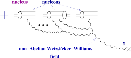
FIG. 1.: Non-Abelian Weizsäcker-Williams field of a large nucleus, as derived in [15, 16, 18].

To describe the saturation philosophy let us start by considering a small-$x$ gluon distribution function of a single ultrarelativistic nucleus. Let us suppose that Bjorken $x$ is small, $x\,\ll\,1$, but not too small for quantum corrections to become important [12, 13]. The quantum corrections at small $x$ bring in the powers of $\alpha_{s}\ln 1/x$ and are resummed for the case of one rescattering by the BFKL equation [14]. If $\alpha_{s}\ln 1/x\,\ll\,1$ we can describe the gluon distribution in the nuclear wave function including multiple rescatterings on the nucleons by the classical gluon field calculated in light cone gauge [10]. The field has been found in [15, 16] and was dubbed the non-Abelian Weizsäcker-Williams field of a large nucleus. In the $A_{+}=0$ light cone gauge (with the nucleus moving in the “plus” direction along the light cone) the field has only transverse components which are given by [15, 16]

$${\underline{A}}^{WW}({\underline{x}},x_{-})\ =\ \int\ d^{2}z\ dz_{-}\theta(z_{-}-x_{-})\ {\hat{\rho}}^{a}({\underline{z}},z_{-})\ \frac{{\underline{x}}-{\underline{z}}}{|{\underline{x}}-{\underline{z}}|^{2}}\ S_{0}({\underline{x}},z_{-})T^{a}S_{0}^{-1}({\underline{x}},z_{-})$$ (1)

with the gauge rotation matrix given by a path-ordered integral

$$S_{0}({\underline{x}},x_{-})\ =\ \mbox{P}\exp\left(igT^{a}\int\ d^{2}z\ dz_{-}\theta(z_{-}-x_{-})\ {\hat{\rho}}^{a}({\underline{z}},z_{-})\ \ln(|{\underline{x}}-{\underline{z}}|\mu)\right).$$ (2)

${\hat{\rho}}^{a}$ is a color charge density operator normalized according to

$$\left<{\hat{\rho}}^{a}({\underline{x}},x_{-})\ {\hat{\rho}}^{b}({\underline{y}},y_{-})\right>\ =\ \frac{\alpha_{s}}{2N_{c}\pi}\,\rho({\underline{x}},x_{-})\,\delta(x_{-}-y_{-})\,\delta^{2}({\underline{x}}-{\underline{y}})\,\delta^{ab}$$ (3)

with $\rho({\underline{x}},x_{-})$ the normal nuclear density in the infinite momentum frame of the nucleus, obeying

$$\int\ d^{2}x\ dx_{-}\ \rho({\underline{x}},x_{-})=\ A.$$ (4)

Here we have used the notation of [17] to describe the non-Abelian Weizsäcker-Williams field. Feynman diagrams corresponding to this classical field were found in [18] and are depicted in Fig. 1. As was discussed in some detail in [18] the multiple rescatterings are included in the non-Abelian Weizsäcker-Williams field in the form of gauge rotations. In Fig. 1 the field of the rightmost nucleon effectively gets rotated by the fields of all the other nucleons in the nucleus (see Fig. 1). As was argued in [18] classical approximation corresponds to the limit of no more than two gluons interacting with each nucleon, which formally means resummation of all powers of the parameter $\alpha_{s}^{2}A^{1/3}$ with $A$ the atomic number of the nucleus. Each additional power of $\alpha_{s}^{2}A^{1/3}$ corresponds to an extra rescattering and resummation of all of such terms corresponds to resummation of multiple rescatterings. For a large nucleus with $\alpha_{s}^{2}A^{1/3}\,\sim\,1$ all multiple rescatterings are important.

The unintegrated gluon distribution function of a nucleus is proportional to Fourier transform of the correlator of two Weizsäcker-Williams fields in the nuclear wave function, which was calculated in [16, 17] and is given by Eq. (26) below. This classical unintegrated gluon distribution has a very peculiar features: at large values of transverse momentum it falls off like $1/k_{\perp}^{2}$, which is a usual perturbative result. As the transverse momentum becomes smaller the distribution increases. However below certain momentum scale, which is called the saturation scale and is given below by Eq. (24), the growth of the classical gluon distribution slows down to just a logarithmic increase, proportional to $\ln Q_{s}/k_{\perp}$. This suggests that multiple rescatterings may help us to avoid the singularities of collinear factorization by introducing the saturation scale $Q_{s}$, which effectively regulates the parton distributions in the soft momentum region. In terms of this saturation scale parameter resummation of multiple rescatterings corresponds to resummation of powers of $Q_{s}^{2}/k^{2}_{\perp}$, since $Q_{s}^{2}\,\sim\,\alpha_{s}^{2}A^{1/3}$ (see Eq. (24)). The scale determining the value of the strong coupling constant $\alpha_{s}$ is also the saturation momentum $Q_{s}$. Therefore applicability of perturbative QCD and quasi-classical physics depends strongly on how big $Q_{s}$ is. If $Q_{s}^{2}\,\gg\,\Lambda_{QCD}^{2}$ then $\alpha_{s}(Q_{s}^{2})\,\ll\,1$ and the physics described above is applicable to the nuclear scattering process.

As the energy increases (or, equivalently, as we go towards smaller values of $x$) the quantum corrections become important. Multiple rescatterings enhanced by quantum corrections become multiple pomeron exchanges. There were developed several techniques which resum multiple pomeron exchanges. The techniques based on resummation of successive classical emissions in the framework of effective lagrangian of McLerran-Venugopalan model led to a renormalization group functional differential equation of [19]. There are different effective lagrangian approaches, such as the one developed by Lipatov and collaborators [20] and another one by Balitsky [21]. Finally there is an integral evolution equation which was obtained in [23] using the techniques of Mueller’s dipole model [22]. The equation is similar to the GLR equation of [11] and was also obtained in [21] for the evolution of the Wilson lines’ correlators. The approach of [19] also seems to be converging to the equation of [23] (see [24]). Nevertheless, as was argued in [25, 10] the net effect of quantum corrections is to increase the saturation scale $Q_{s}$ without significantly changing the shape and main qualitative features of the classical gluon distribution.

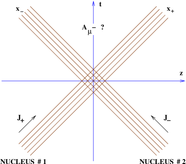
FIG. 2.: A collision of two ultrarelativistic nuclei at high energies.

But what does the saturation physics teach us about the initial conditions for the heavy ion collisions? Similarly to how it was done for the case of a single nucleus structure functions one has to start by considering purely classical case, neglecting the quantum corrections. This of course corresponds to not extremely high energy scattering, $\alpha_{s}\ln s\,\ll\,1$. For realistic high energies one has to include quantum evolution corrections, but classical initial conditions (in the QCD evolution sense) are necessary in order to do so. Quantum corrections may again only modify the saturation scale in the classical distribution without significantly changing its shape, as it happened for nuclear structure functions [25, 10]. The problem of inclusion of quantum corrections still has not been solved. However, since the quantum evolution can be represented as a series of classical emissions [19, 22] the qualitative picture of particle production has been constructed in [26] and certain physical consequences, such as multiplicity correlations in rapidity in the produced particle spectrum have been predicted [26].

The classical gluon production problem for nuclear or hadronic collisions has been formulated in [27] by Kovner, McLerran and Weigert. They consider scattering of two ultrarelativistic nuclei from McLerran-Venugopalan model (see Fig. 2). The valence quarks of the nuclei just pass through each other during the collision without deflection from their straight line light cone trajectories. Corrections to this approximation are proportional to positive powers of $x$, and $x\,\ll\,1$. However, the gluonic field generated by the collision has non-zero field strength in the forward light cone and contributes to the gluon production. If we would like to obtain an expression for the distribution of produced gluon which includes all powers of $\alpha_{s}^{2}A^{1/3}$ (or, equivalently, $Q_{s}/k_{\perp}$), we can do it by solving classical Yang-Mills equation with the ultrarelativistic nuclei providing us with the source current [27]. The gluon field given by the solution of the classical equations of motion in the forward light cone would describe the gluon production (see Fig. 2), and, consequently, the initial conditions for heavy ion collisions. This is the problem we are going to address in this paper.

The classical field of two nuclei in the forward light cone has been found in the usual perturbation theory to order $g^{3}$ in [27, 28, 29]. The answer for the distribution of produced gluons is proportional to $Q_{s1}^{2}Q_{s2}^{2}/k_{\perp}^{4}$, where $Q_{s1}$ and $Q_{s2}$ are the saturation scales of the colliding nuclei. This is the first (lowest order) term of the expansion in powers of $Q_{s1,2}^{2}/k_{\perp}^{2}$ and corresponds in this sense to proton-proton scattering. The answer agrees with the production rate one would get from employing the so-called Lipatov effective vertex [14, 11], or, equivalently, with the result of Gunion and Bertsch [30].

A gluon production cross section for a slightly more complicated case of proton-nucleus interactions was derived in [17]. In the formal language of the saturation scale parameters $Q_{s1}$ and $Q_{s2}$ that cross section includes all powers of $Q_{s1}^{2}/k_{\perp}^{2}$ keeping only the leading power of $Q_{s2}^{2}/k_{\perp}^{2}$.

The problem of finding the classical gluon field in nucleus-nucleus collisions has been addressed in lattice simulations of Krasnitz and Venugopalan [31]. The numerical distribution of the produced particles has been found and exhibited saturation properties expected, such as finiteness in the small transverse momentum limit. Mueller [7] suggested that the total number of the produced gluons has to be proportional to the total number of gluons in the nuclear wave function with the proportionality coefficient $c$ of order one. The numerical value of the coefficient was determined in [31] to be $c=1.29\pm 0.09$.

In this paper we are going to write down an analytical expression for the distribution of produced gluons which resums all powers of both $Q_{s1}^{2}/k_{\perp}^{2}$ and $Q_{s2}^{2}/k_{\perp}^{2}$. That is we are going to address the problem of nucleus-nucleus scattering analytically. The paper is organized as follows: in Sect. II we will formulate the problem of classical gluon production and make some useful observations revealing the advantages and disadvantages of viewing the process in different gauges. In Sect. IIIA we will review the solution of the proton-nucleus (pA) problem in covariant gauge which was given in [17], showing how multiple final state rescatterings play crucial role in gluon production. In Sect. IIIB we will analyze the same process of gluon production in pA collisions in light cone gauge and demonstrate that an entirely different set of initial state interactions is important there. We will outline certain important cancellations of diagrams, which would allow us to write down an expression for the produced gluons’ distribution in nucleus-nucleus (AA) collisions in Sect. IV. This distribution is given by Eq. (40) and is the central result of this paper. It gives the distribution of gluons in the state immediately following a heavy ion collision providing initial condition for possible thermalization of the gluonic system at later times. We explore the properties of the distribution of Eq. (40) in Sect. V. There we first obtain a simplified expression for the distribution in the case of not very large transverse momenta $k_{\perp}\,{{}_{\displaystyle{<}}\atop\displaystyle{\sim}}\,Q_{s}$, which is given by Eq. (43). We demonstrate that the distribution of produced gluons (40) is finite up to $\ln Q_{s}/k_{\perp}$ in the soft transverse momentum limit and scales as $1/k_{\perp}^{4}$ when the transverse momentum gets large. We calculate the typical momentum of the produced gluons and find that for the case of identical nuclei it is of the order of the saturation scale $Q_{s}$, as was conjectured by Mueller in [7]. Finally we estimate the coefficient $c$ from [7] and find $c\,\approx\,2\ln 2$, which is close to the result of [31]. In Sect. VI we estimate the saturation scale using the new data from PHOBOS experiment at RHIC [1] and obtain $Q_{s}^{2}\,\approx\,2\,\mbox{GeV}^{2}$, which is marginally in the perturbative QCD region and agrees with the result of [32]. We end the paper with a summary of the results obtained.

II Formulation of the Problem

In this section we are going to review the formulation of the problem of finding the classical gluon field of two colliding nuclei and make some observations which will be useful later.

As was originally stated in [27] one needs to solve the classical Yang–Mills equations

$$D_{\mu}F^{\mu\nu}=J^{\nu}\,\,,$$ (5)

with the current $J^{\mu}$ arising due to the valence quarks in the colliding nuclei. The valence quarks move ultra-relativistically along the straight lines on the light cone and do not get deflected in the collision. (Deflection is suppressed by a power of the center of mass energy of the colliding system.) Thus the current generated by them has non-zero light cone components $J_{+}$ and $J_{-}$ and zero transverse component ${\underline{J}}\,=\,0$. In a non-Abelian theory the source current is not gauge invariant, it gets rotated under gauge transformations. We will first construct the current in a particular gauge — covariant gauge

$$\partial_{\mu}\,A_{\mu}\,=\,0.$$ (6)

Before the collision the nuclei do not see each other and do not interact. The current is given by the sum of the currents of two free nuclei on the light cone. As was shown in [15, 28] the current of a free nucleus in covariant gauge is given by a simple superposition of the currents of the point color charges (valence quarks) in the nucleus, each of them being parametrically of order $g$ in strong coupling constant. For example, in the model of quarkonium nucleus considered in [15, 28], where the nucleus was envisaged as an ensemble of point color charges, with each nucleon consisting of two valence quarks (a quark and an antiquark), the free current is

$$J_{+}^{cov\ (0)} = g\sum_{i=1}^{A_{1}}T^{a}\,(T_{i}^{a})\,[\delta(x_{-}-x_{i-})\,\delta({\underline{x}}-{\underline{x}}_{i})-\delta(x_{-}-x^{\prime}_{i-})\,\delta({\underline{x}}-{\underline{x}}^{\prime}_{i})]\,\,,$$ (8)

$$J_{-}^{cov\ (0)} = g\sum_{j=1}^{A_{2}}T^{a}\,(\tilde{T}_{j}^{a})\,[\delta(x_{+}-y_{j+})\,\delta({\underline{x}}-{\underline{y}}_{j})-\delta(x_{+}-y^{\prime}_{j+})\,\delta({\underline{x}}-{\underline{y}}^{\prime}_{j})]\,\,,$$ (9)

$${\underline{J}}^{cov\ (0)} = 0\,\,.$$ (10)

Here $x_{i}$’s ($x^{\prime}_{i}$’s) and $y_{j}$’s ($y^{\prime}_{j}$’s) are positions of the quarks (antiquarks) in the $i$th nucleon of the first and in the $j$th nucleon of the second nucleus correspondingly. The first nucleus is moving in the “+” direction, while the second is moving in the “$-$” direction (Fig. 2). $(T_{i}^{a})$ and $(\tilde{T}_{j}^{a})$ are $SU(3)$ color generators of the $i$th nucleon in the first nucleus and of the $j$th nucleon in the second nucleus. $A_{1}$ and $A_{2}$ are the atomic numbers of the nuclei.

Eq. (5) implies conservation of the classical current $J_{\mu}$

$$D_{\mu}\,J_{\mu}\,=\,0.$$ (11)

Similarly to what was done in [28] we will use this condition to construct the covariant gauge current $J^{cov}_{\mu}$ during and after the collision. The valence quarks do not get deflected from their light cone trajectories in the collision. The only non-zero components of the current are therefore $J_{+}$ and $J_{-}$. We can rewrite Eq. (11) as

$$\partial_{+}\,J^{cov}_{-}+\partial_{-}\,J^{cov}_{+}-ig[A^{cov}_{+},J^{cov}_{-}]-ig[A^{cov}_{-},J^{cov}_{+}]=0.$$ (12)

Eq. (12) can be satisfied with the following ansatz for the current

$$J^{cov}_{+}\,=\,U^{-1}(x)\,J^{cov\ (0)}_{+}(x)\,U(x),\hskip 28.45274ptJ^{cov}_{-}\,=\,S^{-1}(x)\,J^{cov\ (0)}_{-}(x)\,S(x),$$ (13)

where

$$U(x)\,=\,\mbox{P}\exp\left(-ig\int_{-\infty}^{x_{+}}\ dx^{\prime}_{+}\ A^{cov}_{-}\right)$$ (14)

and

$$S(x)\,=\,\mbox{P}\exp\left(-ig\int_{-\infty}^{x_{-}}\ dx^{\prime}_{-}\ A^{cov}_{+}\right),$$ (15)

with $A^{cov}_{\pm}$ the components of the unknown solution of Eq. (5). Thus generally speaking the matrices $U(x)$ and $S(x)$ are not known. In arriving at the solution of Eq. (12) given by Eqs. (13), (14) and (15) we have fixed the initial conditions for Eq. (12): we required that before the collision the current $J^{cov}_{\mu}$ should be given by the free nuclear current $J^{cov\ (0)}_{\mu}$ of Eq. (II). This is just a casuality requirement which makes sure that there is no interactions between the nuclei prior to collision. Eqs. (13), (14) and (15) certainly satisfy this initial condition, since before the collision $U\ =\ S\ =\ 1$, as the fields of free nuclei are non-zero only on light cone (see for instance [15, 33]). Since Eq. (12) is a linear differential equation the solution of Eq. (13) is unique for the given initial condition of Eq. (II).

Eq. (13) has a very simple physical interpretation: the valence quarks in the nuclei during and after the collision are still moving along the same straight lines on the light cone. The only effect of the collision on these valence quarks is the rotation of their color charges by the gluon field created in the collision and by the gluon field of the other nucleus. This has been discussed and illustrated in [28] at the lowest nontrivial order in $\alpha_{s}$.

Eqs. (5) and (13) provide us with complete formulation of the problem in covariant gauge. We have to solve the Yang-Mills equations (5) with the conserved current (13). We are now going to demonstrate an interesting property of the current.

Let us perform a gauge transformation with the matrix $S(x)$. The new gluon field will be given by

$$A^{LC}_{\mu}\,=\,S\ A^{cov}_{\mu}S^{-1}\,-\,\frac{i}{g}\ (\partial_{\mu}S)\ S^{-1}.$$ (16)

As easy to see $A^{LC}_{+}\,=\,0$, which means that the gauge transformation with the matrix $S(x)$ transforms the field into the light cone gauge. The current in the light cone gauge is

$$J^{LC}_{+}\,=S(x)\,U^{-1}(x)\,J^{cov\ (0)}_{+}(x)\,U(x)\,S^{-1}(x),\hskip 28.45274ptJ^{LC}_{-}\,=\,J^{cov\ (0)}_{-}(x).$$ (17)

From Eq. (17) it follows that the “$-$” component of the current in the $A^{LC}_{+}\,=\,0$ light cone gauge remains unchanged throughout the collision and is equal to the order $g$ “initial” free nucleus current in the covariant gauge. That means that the charges of the second nucleus in the light cone gauge do not get rotated in the collision. Let us illustrate what this statement means in terms of diagrams.

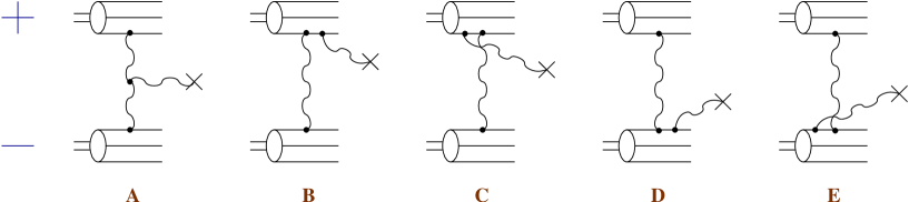
FIG. 3.: Diagrams contributing to the classical gluon field in covariant gauge at order $g^{3}$.

In [27, 28, 29] the classical gluon field of two colliding nuclei was found perturbatively at the lowest non-trivial order in $g$, which happened to be order $g^{3}$. The diagrams contributing to the gluon field at this order in covariant gauge are shown in Fig. 3. There we present a collision of two ultrarelativistic nucleons, the upper one of which is moving in the light cone “plus” direction while the lower one is moving in the “minus” direction. The straight lines in Fig. 3 correspond to the valence quarks. The cross denotes the point in coordinate space where one measures the field.

The interpretation of the diagrams of Fig. 3 has been given in [28]. In diagram A two gluon fields merge to produce the final field. In the diagrams B and C the current of the upper quark gets rotated by the field of the lower quark and a gluon is emitted off the modified current. In the diagrams D and E the opposite happens: the current of the lower quark gets rotated by the field of the upper quark and emits a gluon. In both cases of B,C and D,E the current of one of the quarks gets a rotational correction of the order $g^{2}$ (one gluon exchange contribution) which could also be obtained from Eq. (13) by perturbative expansion of the matrices $U(x)$ and $S(x)$ to the lowest non-trivial order [28].

FIG. 4.: $A_{+}=0$ light cone gauge diagrams: A contributes to the classical gluon field while B does not.

Now looking at the light cone gauge current given by Eq. (17) we see that $J^{LC}_{\mu}$ does not get any rotational corrections whatsoever and remains at the lowest order in $g$ (free nucleus current). Therefore we can conclude that, for instance, diagrams D and E of Fig. 3 do not contribute to the classical gluon field in $A_{+}\ =\ 0$ light cone gauge, which is a self-evident statement. However, we can draw more general and less trivial conclusions from Eq. (17). Since the current of the second nucleus does not get rotated it means that it only rotates the current and/or the field of another nucleus. This also implies that there is no diagrams with more than one gluon line connecting to any quark line in the second nucleus (except for virtual diagrams where two gluons can connect to a single quark line – see [18]). The statement is illustrated in Fig. 4. Diagram in Fig. 4A has only one gluon line attaching to the quark line in the second (lower) nucleus moving in the “minus” direction and therefore may contribute to the classical field. The diagram of Fig. 4B has two gluons interacting with the quark in a nucleon of the second nucleus, and the nucleon remains in a color non-neutral state at the end. This diagram does not contribute to the classical field according to what we have shown in Eq. (17).

III Proton-Nucleus Collisions Revisited

Before addressing the issue of nucleus–nucleus collisions (AA) let us first consider a somewhat easier problem of proton–nucleus collisions (pA). Below we are going to review the solution of the problem in covariant gauge given in [17] and then proceed by analyzing the same pA process in the light cone gauge of the nucleus. Our interpretation of the underlying light cone gauge physics will be slightly different from the one presented in [17].

A Covariant Gauge

Consider a collision of an ultrarelativistic nucleus moving in the “plus” light cone direction and a proton moving in the “minus” light cone direction. For pA collisions we want to solve the same problem of classical gluon production as was stated above for AA collisions. In this subsection we will just follow the discussion of [17]. We will work in $A_{-}\ =\ 0$ gauge with polarization vector also taken in that gauge, $\epsilon_{-}\ =\ 0$, which for the nucleus moving in the “plus” direction is equivalent to covariant gauge ($\partial\cdot A\ =\ 0$) [17]. Following [17] we will consider the process in the rest frame of the nucleus and perform the calculations in the light cone perturbation theory (see [34] and references therein). Then the physical picture of the gluon production is the following: the incoming proton may already have a gluon in its light cone wave function before the collision with the nucleus and the system of the proton and gluon multiply rescatters on the nucleons in the nucleus. Alternatively the proton can emit the gluon after the multiple rescatterings in the nucleus. The diagrams where the gluon is emitted during the proton’s passing through the nucleus are suppressed by powers of its large light cone momentum $p_{-}$, i.e., by powers of center of mass energy of the system (eikonal approximation) [17]. Multiple rescatterings are easier to resum by calculating the amplitude in the transverse coordinate space [13, 17]. To obtain the gluon production cross section we have transform the amplitude into the momentum space and square it. The diagrams contributing to the gluon production cross section are shown in Fig. 5. The graph in Fig. 5A corresponds to the square of the amplitude corresponding to the case when the gluon is present in proton’s wave function before the collision. The diagram in Fig. 5B gives the interference term between the amplitude from Fig. 5A and the amplitude in which the gluon is emitted by the proton after the collision. Of course a diagram complex conjugate to Fig. 5B should also be included. It can be shown that the square of the diagram with late gluon emission does not have any interactions in it and can be neglected. (The gluon exchanges between the proton and the nucleus cancel.) In [17] the interactions counting was a little different from the one we will present below and that diagram was included, leading to the same result.

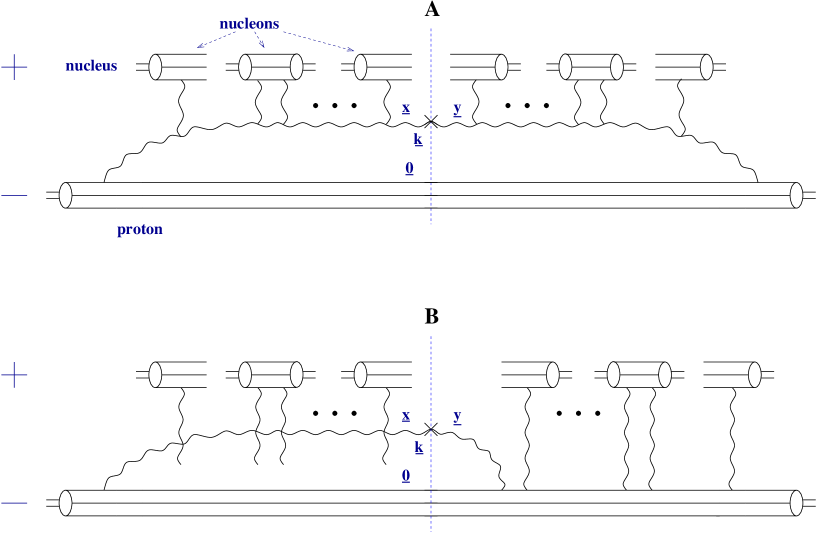
FIG. 5.: Covariant gauge (or more accurately $A_{-}=0$ gauge) gluon production diagrams for proton–nucleus collision as considered in [17]. Multiple rescatterings in the nucleus determine the interactions in this gauge.

Note also that in the quasi–classical approximation depicted in Fig. 5 the interaction is modeled by single and double gluon exchanges. The limit of no more than two gluons per nucleon is imposed [18]. If a particular nucleon exchanges a gluon with the rest of the system in the amplitude then it has to exchange a gluon in the complex conjugate amplitude to remain color neutral. Alternatively the nucleon can exchange two gluon in the amplitude (complex conjugate amplitude) , but then it can not interact in the complex conjugate amplitude (amplitude). This is done in the spirit of the quasi–classical approximation resumming all powers of $\alpha_{s}^{2}\ A^{1/3}$, as was discussed in the Introduction.

In the graph of Fig. 5A the nucleons of the nucleus interact with both the proton and the gluon by gluon exchanges. It was noticed in [17] that the interactions with the proton can be neglected due to real–virtual cancellation. Moving a gluon exchanged between the nucleus and the proton across the cut does not change the momentum of the produced gluon in Fig. 5A but does change the sign of the whole term, causing the cancellation. That is why we have to consider only the interactions with the gluon in Fig. 5A. Similar kind of cancellation does not happen in Fig. 5B. Moving an exchanged (Coulomb) gluon across the cut would force us to move it across the gluon emission vertex for the produced gluon on the right hand side, thus changing the momentum of the produced gluon. Thus all the possible interactions have to be included in Fig. 5B. On the right hand side of the diagram in Fig. 5B only the interactions with the proton are possible.

To obtain the answer for the gluon production cross section in pA in the quasi–classical approximation we have to convolute the wave function of the proton with a soft gluon in it with the Glauber-type propagator. The answer has been derived in [17] (see also [35] and references therein). The diagram in Fig. 5A gives [17]

$$\frac{d\sigma^{pA}_{1}}{d^{2}k\ dy}\ =\ \frac{1}{\pi}\,\int\ d^{2}b\,d^{2}x\,d^{2}y\,\frac{1}{(2\pi)^{2}}\,\frac{\alpha_{s}C_{F}}{\pi}\frac{{\underline{x}}\cdot{\underline{y}}}{{\underline{x}}^{2}{\underline{y}}^{2}}\,e^{i{\underline{k}}\cdot({\underline{x}}-{\underline{y}})}\,\left(e^{-({\underline{x}}-{\underline{y}})^{2}\ Q_{s}^{2}/4}-1\right)$$ (19)

and the diagram in Fig. 5B plus its complex conjugate after a somewhat more sophicticated calculation [17] gives [17]

$$\frac{d\sigma^{pA}_{2+3}}{d^{2}k\ dy}\ =\ \frac{1}{\pi}\,\int\ d^{2}b\,d^{2}x\,d^{2}y\,\frac{1}{(2\pi)^{2}}\,\frac{\alpha_{s}C_{F}}{\pi}\frac{{\underline{x}}\cdot{\underline{y}}}{{\underline{x}}^{2}{\underline{y}}^{2}}\,e^{i{\underline{k}}\cdot({\underline{x}}-{\underline{y}})}\,\left(1-e^{-{\underline{x}}^{2}\ Q_{s}^{2}/4}+1-e^{-{\underline{y}}^{2}\ Q_{s}^{2}/4}\right).$$ (20)

The total gluon production cross section is equal to the sum of the terms in Eq. (5)

$$\frac{d\sigma^{pA}}{d^{2}k\ dy}\ =\ \frac{d\sigma^{pA}_{1}}{d^{2}k\ dy}+\frac{d\sigma^{pA}_{2+3}}{d^{2}k\ dy}.$$ (21)

In Eq. (5) ${\underline{x}}$ and ${\underline{y}}$ are the transverse coordinates of the gluon in the amplitude and the complex conjugate amplitude correspondingly counted with respect to the transverse position of the quark in the proton off which the gluon is emitted (${\underline{0}}$). $b$ is the impact parameter. ${\underline{k}}$ is the gluon’s transverse momentum. Same as in [17] we use a shorthand notation (see also [13])

$${\underline{x}}^{2}Q_{s}^{2}\ =\ {\underline{x}}^{2}\ \frac{8\pi^{2}\alpha_{s}N_{c}R}{N^{2}_{c}-1}\,\rho\,xG(x,1/{\underline{x}}^{2}),$$ (22)

with $\rho$ the density of Eq. (4) taken in the nuclear rest frame. In the two gluon approximating the gluon distribution function of a nucleon is

$$xG(x,1/{\underline{x}}^{2})\ =\ \frac{\alpha_{s}C_{F}}{\pi}\,\ln\frac{1}{{\underline{x}}^{2}\mu^{2}},$$ (23)

with $\mu$ some infrared cutoff. For simplicity of calculations throughout the paper we assume that the nucleus has a cylindrical shape, with radius $R$ and the height of the cylinder $2R$. The cylinder is lined up along the $z$ axis. Generalization of our results to a spherical nucleus is trivial.

In general the saturation scale $Q_{s}^{2}$ has to be found from the following implicit equation [17, 13]

$$Q_{s}^{2}\ =\ \frac{8\pi^{2}\alpha_{s}N_{c}R}{N^{2}_{c}-1}\,\rho\,xG(x,Q_{s}^{2}).$$ (24)

However, since the logarithm in Eq. (23) is a slowly varying function we can assume that in our classical approximation without any QCD evolution in the structure functions the gluon distribution function is approximately a constant and the right hand side of Eq. (24) is independent of $Q_{s}$. Thus Eq. (24) turns from implicit equation into an equality.

To summarize the results reviewed here we note that the gluon production in pA collisions in covariant gauge is driven by the multiple final state interactions. Now we will explore how this picture changes in the light cone gauge of the nucleus.

B Light Cone Gauge

Let us now consider pA scattering in the $A_{+}=0$ light cone gauge with polarization vector also taken in the same gauge $\epsilon_{+}\ =\ 0$. A direct analysis of the light cone gauge diagrams could be a little difficult [17]. We are going to use a different strategy, which was already employed previously in [18]. We know the answer for the gluon production cross section given by Eq. (5). Here we are going to guess the diagrams in the $A_{+}=0$ light cone gauge which give us the same answer. Once we guessed the correct diagrams we can conclude that the remaining diagrams should cancel with each other, since they do not contribute to the cross section.

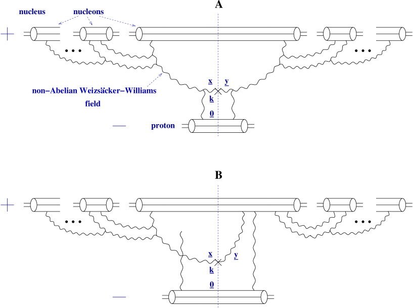
FIG. 6.: Gluon production in proton–nucleus collisions in $A_{+}=0$ light cone gauge (see text).

The light cone gauge diagrams contributing to the gluon production cross section in proton–nucleus collisions are depicted in Fig. 6. The pA scattering process could be viewed in either rest frame of the proton or in the center of mass frame. Again we are going to perform the calculation in the framework of the light cone perturbation theory. Similar to the covariant gauge case considered above the incoming nucleus can emit a gluon in its wave function either before or after the collision with the proton. The one gluon light cone wave function of an ultrarelativistic nucleus is given by ${\underline{A}}^{WW}({\underline{x}})\cdot{\underline{\epsilon}}$, with ${\underline{A}}^{WW}$ the non-Abelian Weizsäcker-Williams field of the nucleus given by Eq. (1) with suppressed $x_{-}$ dependence [15, 16] and ${\underline{\epsilon}}$ the polarization vector in light cone gauge. (One can see that it is the case for instance by calculating the one gluon rescattering diagram on the left hand side of Fig. 6A with this wave function and by using conventional perturbation theory. Both results give the same answer.) Diagrammatically the light cone wave function corresponds to the same set of diagrams as was depicted above in Fig. 1. The fields of the nucleons in the nucleus “gauge rotate” the Weizsäcker-Williams field of one of the nucleons [18]. The interaction with the proton can only be by the means of single or double gluon exchanges, as was shown in Sect. II. Eq. (17) shows that the “minus” component of the current does not get rotated implying that there could not be more than two gluons exchanged with the proton in the $A_{+}=0$ light cone gauge.

Before colliding with the proton the nucleus can develop the Weizsäcker-Williams one gluon light cone wave function which then interacts with the proton by means of one or two gluon exchanges, according to the rules of the quasi–classical approximation [18, 17]. The square of the graph corresponding to this scenario is shown in Fig. 6A. As in Fig. 5 the interactions of the proton with the nucleons in the nucleus cancel through the real–virtual cancellation leaving only the interactions with the gluon line. One may notice that the final state interactions are left out in the diagram of Fig. 6A, but as we will show below we do not need them to reproduce the contribution of the graph in Fig. 5A, which implies that they cancel with each other.

The second possible scenario corresponds to the case when there is no gluon in the nuclear wave function by the time the collision happens and the gluon is emitted by the nucleus after the interaction with the proton. Then the nuclear wave function without an emitted gluon corresponds to the fields of the nucleons rotating the current of one of the nucleons in the nucleus. This is shown on the right hand side of Fig. 6B. The nucleon then interacts with the proton by exchanging one or two gluons with it. After that the nucleus can emit a gluon to be produced in the final state. Another possibility which is not shown in Fig. 6B but which contributes to the gluon production corresponds to the case when the Weizsäcker-Williams gluon is present in the nuclear wave function by the time of the collision, similar to Fig. 6A, but after the interaction with the proton the gluon merges into the quark line of one of the nucleons, which later re-emits the gluon. We could not find an a priori argument prohibiting an emission of the whole Weizsäcker-Williams field after the interaction. However, as we will see below one needs to emit only one gluon to be able to reproduce the results of the previous section. The square of the diagram on the right hand side of Fig. 6B is zero since the interactions cancel due to real–virtual cancellation [17]. The only contribution we get from it is the interference term depicted in Fig. 6B. There on the left hand side we have the same diagram as in Fig. 6A except that now interactions of the proton with the “last” nucleon in the nucleus do not cancel. We will show that the diagram of Fig. 6B provides us with the contribution equal to that of the graph in Fig. 5B.

Let us now calculate the diagrams in Fig. 6. The contribution of Fig. 6A can be obtained by convoluting the correlation function of the fields on both sides of the cut with the gluon–proton interactions amplitude. The result yields

$$\frac{d\sigma^{pA}_{LC1}}{d^{2}k\ dy}\ =\ \int\frac{d^{2}x\ d^{2}y}{(2\pi)^{2}}\,e^{i{\underline{k}}\cdot({\underline{x}}-{\underline{y}})}\,\frac{2}{\pi}\,\mbox{Tr}\,\left<{\underline{A}}^{WW}({\underline{x}})\cdot{\underline{A}}^{WW}({\underline{y}})\right>\,\frac{-\alpha_{s}\pi^{2}N_{c}}{N_{c}^{2}-1}\,({\underline{x}}-{\underline{y}})^{2}\,xG(x,1/({\underline{x}}-{\underline{y}})^{2}).$$ (25)

In [16, 17] the correlation function of two non-Abelian Weizsäcker-Williams fields in the nuclear wave function was found to be

$$\mbox{Tr}\left<{\underline{A}}^{WW}({\underline{x}})\cdot{\underline{A}}^{WW}({\underline{y}})\right>\,=\,\frac{C_{F}}{\pi\alpha_{s}({\underline{x}}-{\underline{y}})^{2}}\,\left(1-e^{-({\underline{x}}-{\underline{y}})^{2}\,Q_{s}^{2}/4}\right).$$ (26)

Employing Eqs. (26) and (23) in Eq. (25) and defining new variables ${\underline{z}}={\underline{x}}-{\underline{y}}$ and ${\underline{b}}={\underline{y}}$ we obtain

$$\frac{d\sigma^{pA}_{LC1}}{d^{2}k\ dy}\ =\ \int\,d^{2}b\,d^{2}z\,e^{i{\underline{k}}\cdot{\underline{z}}}\,\frac{1}{(2\pi)^{2}}\,\frac{\alpha_{s}C_{F}}{\pi}\,\ln\frac{1}{{\underline{z}}^{2}\mu^{2}}\,\left(e^{-{\underline{z}}^{2}\,Q_{s}^{2}/4}-1\right).$$ (27)

Using Eqs. (63) and (64) from [17] one can see that

$$\ln\frac{1}{{\underline{z}}^{2}\mu^{2}}\,=\,\frac{1}{\pi}\,\int d^{2}y\,\frac{{\underline{y}}\cdot({\underline{z}}+{\underline{y}})}{{\underline{y}}^{2}({\underline{z}}+{\underline{y}})^{2}}$$ (28)

where the $y$ integration is cut off by $1/\mu$ in the infrared limit. Inserting Eq. (28) into Eq. (27) and comparing the result to Eq. (5a) one can see that

$$\frac{d\sigma^{pA}_{LC1}}{d^{2}k\ dy}\ =\ \frac{d\sigma^{pA}_{1}}{d^{2}k\ dy}.$$ (29)

Thus we have shown that the contribution of the diagrams in Fig. 6A is equal to the contribution of the diagrams in Fig. 5A.

The calculation of the graphs depicted in Fig. 6B is a little more complicated. Similar to diagrams of Fig. 6A a correlator of two gluonic fields is involved. However, in the field on the right hand side of the cut in Fig. 6B only rotations of the source are allowed. Similarly to what was done in [18, 17] we argue that the fields of the nucleons rotate the quark line to which the emitted final state gluon is attached, as well as the Coulomb gluon’s field coming from the proton below. Everything is gauge rotated, except for the gluon line of the emitted gluon. After applying Ward identities we conclude that effectively only the vertex where the emitted gluon connects to the quark line on the right hand side of Fig. 6B is rotated. This corresponds to rotation of the source of the gluon field emitted [18]. The effect of this gauge rotation is modification of the expression for the field from Eq. (1) into

$${\underline{A}}^{WW}_{mod}({\underline{x}},x_{-})\ =\ \int\ d^{2}z\ dz_{-}\theta(z_{-}-x_{-})\ {\hat{\rho}}^{a}({\underline{z}},z_{-})\ \frac{{\underline{x}}-{\underline{z}}}{|{\underline{x}}-{\underline{z}}|^{2}}\ S_{0}({\underline{z}},z_{-})T^{a}S_{0}^{-1}({\underline{z}},z_{-}).$$ (30)

After we sum over the all possible connections of the Coulomb gluon lines to the “last” nucleon in the nucleus in Fig. 6B the resulting expression would depend on the transverse coordinate of the quark in that nucleon to which the Coulomb gluon couples. Thus we can not factorize the averaging in the nuclear wave function from the interaction terms anymore, like it was done in obtaining Eq. (25). With all the above-mentioned complications in mind we write the contribution of the diagram in Fig. 6B as (see [17] for a similar calculation)

$$\frac{d\sigma^{pA}_{LC2}}{d^{2}k\ dy}\ =\ \frac{2}{\pi}\,\int\frac{d^{2}x\ d^{2}y}{(2\pi)^{2}}\,e^{i{\underline{k}}\cdot({\underline{x}}-{\underline{y}})}\,\int d^{2}z\,dz_{-}\,d^{2}z^{\prime}\,dz^{\prime}_{-}\,\left<\frac{{\underline{x}}-{\underline{z}}}{|{\underline{x}}-{\underline{z}}|^{2}}\cdot\frac{{\underline{y}}-{\underline{z}^{\prime}}}{|{\underline{y}}-{\underline{z}^{\prime}}|^{2}}\,{\hat{\rho}}^{a}({\underline{z}},z_{-})\,{\hat{\rho}}^{b}({\underline{z}}^{\prime},z^{\prime}_{-})\right.$$

$$\left.\times\mbox{Tr}\left[S_{0}({\underline{x}},z_{-})T^{a}S_{0}^{-1}({\underline{x}},z_{-})S_{0}({\underline{z}}^{\prime},z^{\prime}_{-})T^{b}S_{0}^{-1}({\underline{z}}^{\prime},z^{\prime}_{-})\right]\,\frac{\alpha_{s}\pi^{2}N_{c}}{N_{c}^{2}-1}\,({\underline{x}}-{\underline{z}})^{2}\,xG(x,1/({\underline{x}}-{\underline{z}})^{2})\right>$$ (31)

Similar to what was done before in [15, 17] we argue that we can average the densities ${\hat{\rho}}^{a}({\underline{z}},z_{-})\,{\hat{\rho}}^{b}({\underline{z}}^{\prime},z^{\prime}_{-})$ in the nuclear wave function independently and we can employ Eq. (3) to do so. In [17] the following result was derived (see Eq. (48) in [17])

$$\left<\mbox{Tr}\left[S_{0}({\underline{x}},z_{-})T^{a}S_{0}^{-1}({\underline{x}},z_{-})S_{0}({\underline{z}},z_{-})T^{a}S_{0}^{-1}({\underline{z}},z_{-})\right]\right>\ =$$

$$=\ C_{F}N_{c}\exp\left(-\frac{\alpha_{s}\pi^{2}N_{c}}{N_{c}^{2}-1}\,({\underline{x}}-{\underline{z}})^{2}\,\rho({\underline{x}},z_{-})\,xG(x,1/({\underline{x}}-{\underline{z}})^{2})\,(z_{-}+z_{0-})\right),$$ (32)

with $\pm z_{0-}$ is the upper (lower) limit of the $z_{-}$ integration in Eq. (31). In Eq. (32) we assume that $\rho({\underline{x}},z_{-})$ does not vary much between ${\underline{x}}$ and ${\underline{z}}$, which is justified for a large nucleus. Using Eqs. (3) and (32) in Eq. (31) we obtain

$$\frac{d\sigma^{pA}_{LC2}}{d^{2}k\ dy}\ =\ \frac{1}{\pi}\,\int\frac{d^{2}x\ d^{2}y}{(2\pi)^{2}}\,e^{i{\underline{k}}\cdot({\underline{x}}-{\underline{y}})}\,d^{2}z\,\frac{\alpha_{s}C_{F}}{\pi}\,\frac{{\underline{x}}-{\underline{z}}}{|{\underline{x}}-{\underline{z}}|^{2}}\cdot\frac{{\underline{y}}-{\underline{z}}}{|{\underline{y}}-{\underline{z}}|^{2}}\,\left(1-e^{-({\underline{x}}-{\underline{z}})^{2}\,Q_{s}^{2}/4}\right).$$ (33)

Defining new variables ${\underline{x}}={\underline{x}}-{\underline{z}}$, ${\underline{y}}={\underline{y}}-{\underline{z}}$ and ${\underline{b}}={\underline{z}}$ and adding the contribution of the complex conjugate to Fig. 6B diagram ($d\sigma^{pA}_{LC3}/d^{2}k\ dy$) we can compare the result with Eq. (5b) and conclude that

$$\frac{d\sigma^{pA}_{LC2}}{d^{2}k\ dy}+\frac{d\sigma^{pA}_{LC3}}{d^{2}k\ dy}\ =\ \frac{d\sigma^{pA}_{2+3}}{d^{2}k\ dy}.$$ (34)

We have thus shown that the contribution of the diagrams in Fig. 6B is equal to the contribution of the diagrams in Fig. 5B.

We have proved that the diagrams in Fig. 6 are the only diagrams contributing to the gluon production cross section in $A_{+}=0$ light cone gauge. Thus a whole class of diagrams with final state interactions does not contribute to the cross section. Several examples of such graphs are shown in Fig. 7.

The diagram in Fig. 7A represents a class of diagrams where the non-Abelian Weizsäcker-Williams wave function of the nucleus after interaction with the proton merges with another (non-interacting) Weizsäcker-Williams wave function. The graph in Fig. 7B can be viewed as a similar to Fig. 7A process, where after proton-nucleon interaction a gluon field is emitted, which later on merges with the non-Abelian Weizsäcker-Williams wave function of the nucleus. There is another class of diagrams which do not contribute to the cross section where two Weizsäcker-Williams wave functions merge with each other and with a Coulomb gluon coming from the proton through a four-gluon vertex, producing a gluon in the final state. Those diagrams are probably suppressed in the old-fashioned light cone perturbation theory as requiring the gluon fields’ merger to happen at a particular light cone time when the system is passing the proton.

As was shown above all of the final state interactions shown in Fig. 7 do not contribute to the gluon production cross section in pA collisions. Therefore they should cancel, either with each other or individually due to some other cancellation mechanism. From considering gluon production in pA collisions in the light cone gauge we may draw the following conclusion: the gluons produced by the collision do not merge with the non-Abelian Weizsäcker-Williams wave function of the nucleus.

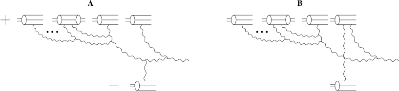
FIG. 7.: Some of the final state interaction diagrams which do not contribute to gluon production in pA collisions in $A_{+}=0$ light cone gauge.

Another important diagram which a priori should be contributing to the gluon production in pA scattering is shown in Fig. 8. The diagram contains virtual interaction between the proton and the field of the nucleus. Even though there is no interaction on the right hand side of the diagram it is allowed by the ruled of the old fashioned light cone perturbation theory, where the energy is not conserved in the vertices [17, 34]. The diagram of Fig. 8 has a remarkable feature in it, which was absent in the graphs shown in Fig. 7: merger of two produced gluons. In Fig. 8 two Weizsäcker-Williams wave functions of the nucleus first interact with the proton producing gluons, which then merge with each other. This merging is different from the ones considered in Fig. 7. There one of the merging gluons was produced in the interaction with the proton while the other one was just given by the non-interacting Weizsäcker-Williams wave function of the nucleus. In Fig. 8 both merging gluons were first “produced” by the interactions and then merged together. Here again, since the diagram of Fig. 8 does not contribute to the gluon production cross section it has to either be zero or cancel with some other diagrams. This gives us a very strong reason to conclude that the gluons produced during the collision do not merge with each other at later times in $A_{+}=0$ light cone gauge. Even a more general conclusion can be conjectured: gluons produced in the interactions do not interact with any other gluons afterwards in $A_{+}=0$ gauge.

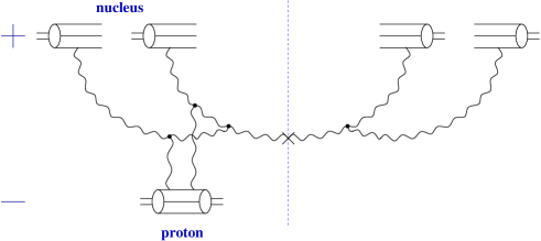
FIG. 8.: A virtual diagram which does not contribute to the gluon production process in pA collisions in $A_{+}=0$ light cone gauge. Triple gluon vertices are marked with black dots.

To conclude we note that the physical interpretation of the scattering process appears to be gauge dependent: in the covariant gauge case considered in the previous section the gluon production was dominated by multiple final state rescatterings. In the light cone gauge multiple rescatterings vanish. The information about them is now contained in the light cone wave function of the nucleus. The same observation about the interplay of initial and final state interactions was made in [17] for the case of current–nucleus scattering with the current $j=-\frac{1}{4}F^{a\,2}_{\mu\nu}$.

IV Nucleus–Nucleus Collisions

Now we can employ the results we have obtained in Sect. III to write down an ansatz for the distribution of produced gluons in nucleus–nucleus collisions. Let us consider a head-on central collision of two ultrarelativistic nuclei, as was shown in Fig. 2. We will be working in $A_{+}=0$ light cone gauge. The calculations can be done either in the center of mass frame or in the rest frame of one of the nuclei. We will work in the rest frame of the second nucleus. The diagrams contributing to gluon production in AA are depicted in Fig. 9. They are somewhat similar to the diagrams of Fig. 6 and of Fig. 5. The incoming nucleus may or may not have a Weizsäcker-Williams gluon in it. In the first case the system multiply rescatters in the second nucleus at rest. This is illustrated in Fig. 9A. Similar to pA case multiple rescatterings between the first and the second nuclei cancel. Only the interactions with the gluon survive. The interference graph of the amplitude from Fig. 9A and the amplitude where the gluon is emitted after the interaction is shown in Fig. 9B. Analogous to pA case we work with diagrams where the final state interactions are limited to multiple rescatterings in the second nucleus and a single gluon emission (or absorption) by the first nucleus. As was demonstrated in Sect. III in the case of proton-nucleus scattering all other final state interactions including “produced” gluons’ merging cancel. Here we argue that this also happens in the nucleus-nucleus collisions.

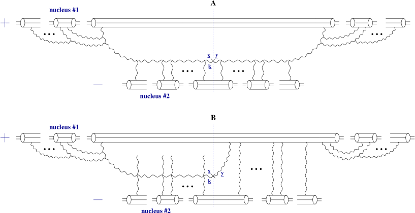
FIG. 9.: Diagrams contributing to the gluon production in nucleus-nucleus collisions in the $A_{+}=0$ light cone gauge.

In Sect. III, analyzing proton-nucleus scattering we concluded that the diagrams where the gluon produced by interaction with the proton merges with the non-Abelian Weizsäcker-Williams wave function of the nucleus cancel. That allowed us to neglect similar diagrams in Fig. 9 above. However, there exists also a somewhat different class of diagrams, one of which is shown in Fig. 10. There the gluons that merge in the later stages of the collision both were produced in the interaction of the Weizsäcker-Williams wave function with the second nucleus. This brings us back to the class of diagrams depicted in Fig. 8, where there is also a merger of two “produced” gluons. Since the diagrams of Fig. 8 canceled in the case of pA collisions we have a strong reason to believe that the graphs of the type shown in Fig. 10 also cancel in AA collisions. Thus Fig. 9 contains all the diagrams that contribute to gluon production in nucleus-nucleus collisions.

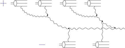
FIG. 10.: An example of a diagram which is not included in the gluon production mechanism of Fig. 9. To avoid possible confusion the three gluon vertices in this diagram are marked by black dots.

We can calculate the diagrams in Fig. 9 along the lines outlined in the previous section. The contribution of the graphs of Fig. 9A is obtained by a simple eikonalization of Eq. (25), and, correspondingly Fig. 6A. The result for the number distribution of the produced gluons yields

$$\frac{dN^{AA}_{1}}{d^{2}k\,dy}\ =\ \int\frac{d^{2}x\ d^{2}y}{(2\pi)^{2}}\,e^{i{\underline{k}}\cdot({\underline{x}}-{\underline{y}})}\,\frac{2}{\pi}\,\mbox{Tr}\,\left<{\underline{A}}_{1}^{WW}({\underline{x}})\cdot{\underline{A}}_{1}^{WW}({\underline{y}})\right>_{1}\,\left(e^{-({\underline{x}}-{\underline{y}})^{2}\,Q_{s2}^{2}/4}-1\right).$$ (35)

Here the indices $1$ and $2$ denote the fields and the saturation scales of the first and the second nuclei correspondingly, as well as over which nucleus wave function the quantities are being averaged. With the help of Eq. (26) we rewrite Eq. (35) as

$$\frac{dN^{AA}_{1}}{d^{2}k\,dy}\ =\ -\frac{2\,C_{F}}{\alpha_{s}\pi^{2}}\,\int\frac{d^{2}x\ d^{2}y}{(2\pi)^{2}}\,e^{i{\underline{k}}\cdot({\underline{x}}-{\underline{y}})}\,\frac{1}{|{\underline{x}}-{\underline{y}}|^{2}}\,\left(1-e^{-({\underline{x}}-{\underline{y}})^{2}\,Q_{s1}^{2}/4}\right)\,\left(1-e^{-({\underline{x}}-{\underline{y}})^{2}\,Q_{s2}^{2}/4}\right).$$ (36)

As was demonstrated in Appendix A of [17] multiple rescatterings of Fig. 9B also just exponentiate. Therefore, in order to calculate the contribution of the diagram of Fig. 9B we should substitute

$$\frac{\alpha_{s}\pi^{2}N_{c}}{N_{c}^{2}-1}\,({\underline{x}}-{\underline{z}})^{2}\,xG(x,1/({\underline{x}}-{\underline{z}})^{2})$$ (37)

in Eq. (31) by

$$1-e^{-({\underline{x}}-{\underline{z}})^{2}\,Q_{s2}^{2}/4}.$$ (38)

Performing all the same integrations and averaging that were done in obtaining Eq. (33) we end up with

$$\frac{dN^{AA}_{2}}{d^{2}k\,dy}\ =\ \frac{2\,C_{F}}{\alpha_{s}\pi^{2}}\,\int\frac{d^{2}x\ d^{2}y}{(2\pi)^{3}}\,e^{i{\underline{k}}\cdot({\underline{x}}-{\underline{y}})}\,d^{2}b\,\frac{{\underline{x}}}{{\underline{x}}^{2}}\cdot\frac{{\underline{y}}}{{\underline{y}}^{2}}\,\frac{1}{{\underline{x}}^{2}\,\ln\frac{1}{|{\underline{x}}|\mu}}\,\left(1-e^{-{\underline{x}}^{2}\,Q_{s1}^{2}/4}\right)\,\left(1-e^{-{\underline{x}}^{2}\,Q_{s2}^{2}/4}\right).$$ (39)

To get the full answer we have to add the contribution of the diagram which is complex conjugate to the one shown in Fig. 9B. Summing up Eqs. (36), (39) and its complex conjugate, we obtain the expression for the number distribution of gluons produced in a heavy ion collision

$$\frac{dN^{AA}}{d^{2}k\,d^{2}b\,dy}\ =\ \frac{2\,C_{F}}{\alpha_{s}\pi^{2}}\,\left\{-\int\frac{d^{2}z}{(2\pi)^{2}}\,e^{i{\underline{k}}\cdot{\underline{z}}}\,\frac{1}{{\underline{z}}^{2}}\,\left(1-e^{-{\underline{z}}^{2}\,Q_{s1}^{2}/4}\right)\,\left(1-e^{-{\underline{z}}^{2}\,Q_{s2}^{2}/4}\right)+\right.$$

$$+\left.\int\frac{d^{2}x\ d^{2}y}{(2\pi)^{3}}\,e^{i{\underline{k}}\cdot({\underline{x}}-{\underline{y}})}\,\frac{{\underline{x}}}{{\underline{x}}^{2}}\cdot\frac{{\underline{y}}}{{\underline{y}}^{2}}\,\left[\frac{1}{{\underline{x}}^{2}\,\ln\frac{1}{|{\underline{x}}|\mu}}\,\left(1-e^{-{\underline{x}}^{2}\,Q_{s1}^{2}/4}\right)\,\left(1-e^{-{\underline{x}}^{2}\,Q_{s2}^{2}/4}\right)+\right.\right.$$

$$+\left.\left.\frac{1}{{\underline{y}}^{2}\,\ln\frac{1}{|{\underline{y}}|\mu}}\,\left(1-e^{-{\underline{y}}^{2}\,Q_{s1}^{2}/4}\right)\,\left(1-e^{-{\underline{y}}^{2}\,Q_{s2}^{2}/4}\right)\right]\right\}.$$ (40)

Eq. (40) is our main result. It provides us with the number of gluons produced in a head-on zero impact parameter heavy ion collision per unit transverse momentum phase space, per unit rapidity interval at the given impact parameter $b$. Eq. (40) includes the nucleon-nucleon scattering result of Fig. 3 calculated in [27, 28, 29] as well as the proton-nucleus scattering contribution of Fig. 6 found in [17]. We are going to explore the properties of the distribution (40) in the next section.

V Properties of the Classical Distribution

Let us evaluate Eq. (40) in the approximation in which we neglect all the logarithms of the transverse coordinates [17], since logarithm is a slowly varying function and can be assumed to be a constant compared to powers. That technically means putting $\ln\frac{1}{|{\underline{x}}|\mu}\,\sim\,\ln\frac{1}{|{\underline{y}}|\mu}\,\sim\,1$ in Eq. (40). That also concerns terms like ${\underline{x}}^{2}\,Q_{s}^{2}$, which in general also have logarithms of $|{\underline{x}}|$ in them, as follows from Eqs. (22) and (23). There we also put the logarithms to be of the order of one, similar to how it was done in [17]. We have to note that this approximation is good only for not very large transverse momenta $k_{\perp}{{}_{\displaystyle{<}}\atop\displaystyle{\sim}}Q_{s}$. When gluon’s momentum is large, $k_{\perp}\gg Q_{s}$, the logarithms of the transverse coordinate are crucial for deriving the correct asymptotics of the distribution function of Eq. (40).

Employing the fact that

$$\int\frac{d^{2}y}{(2\pi)^{2}}\,e^{-i{\underline{k}}\cdot{\underline{y}}}\,\frac{{\underline{y}}}{{\underline{y}}^{2}}\,=\,-\frac{i}{2\pi}\,\frac{{\underline{k}}}{{\underline{k}}^{2}}$$ (41)

in the second term of Eq. (40), integrating over the angles of ${\underline{z}}$ and ${\underline{x}}$ and performing similar integrations in the third term of Eq. (40) we get

$$\frac{dN^{AA}}{d^{2}k\,d^{2}b\,dy}\ =\ \frac{C_{F}}{\alpha_{s}\pi^{3}}\,\int_{0}^{\infty}\frac{dx}{x}\,J_{2}(kx)\,\left(1-e^{-{\underline{x}}^{2}\,Q_{s1}^{2}/4}\right)\,\left(1-e^{-{\underline{x}}^{2}\,Q_{s2}^{2}/4}\right).$$ (42)

Integrating over $x$ in Eq. (42) we find

$$\frac{dN^{AA}}{d^{2}k\,d^{2}b\,dy}\ =\ \frac{C_{F}}{\alpha_{s}2\pi^{3}}\,\frac{1}{{\underline{k}}^{2}}\,\left[(Q_{s1}^{2}+Q_{s2}^{2})\,e^{-\frac{{\underline{k}}^{2}}{Q_{s1}^{2}+Q_{s2}^{2}}}-Q_{s1}^{2}\,e^{-\frac{{\underline{k}}^{2}}{Q_{s1}^{2}}}-Q_{s2}^{2}\,e^{-\frac{{\underline{k}}^{2}}{Q_{s2}^{2}}}\right].$$ (43)

The distribution of Eq. (43) is plotted in Fig. 11 as a function of $k/Q_{s}$ for the case of two identical cylindrical nuclei with $Q_{s1}=Q_{s2}=Q_{s}$ and with the cross sectional area $S_{\perp}\,=\,\pi\,R^{2}\,\approx\,50\,\mbox{fm}^{2}\,\approx\,1250\,\mbox{GeV}^{-2}$. Note again that Eq. (43) is valid only in the not very large transverse momentum region $k_{\perp}{{}_{\displaystyle{<}}\atop\displaystyle{\sim}}Q_{s}$.

FIG. 11.: Distribution of the produced gluons given by Eq. (43) for a central AA collision as a function of $k/Q_{s}$ with the transverse area of the nuclei being $S_{\perp}=50\,\mbox{fm}^{2}$. The approximation of Eq. (40) is valid only for $k_{\perp}\,\ll\,Q_{s}$.

As one can see the distribution in Fig. 11 remains finite as $k_{\perp}/Q_{s}\rightarrow 0$. If one takes the $k_{\perp}\,\ll\,Q_{s}$ limit of Eq. (43) then the distribution goes to a constant

$$\frac{dN^{AA}}{d^{2}k\,d^{2}b\,dy}\ \rightarrow\ \ \frac{C_{F}}{\alpha_{s}2\pi^{3}}\hskip 28.45274pt\mbox{as}\hskip 28.45274pt\frac{k_{\perp}}{Q_{s}}\,\ll\,1.$$ (44)

This means that the exact expression of Eq. (40) may only have logarithmic divergences in the infrared limit. This conclusion is very interesting, since the initial conditions for heavy ion collisions which are generated by pairwise interactions between nucleons in nuclei without multiple rescatterings have a power-law divergences in the infrared limit [8]. Even the pA gluon production cross section of Eq. (5) diverges as $1/k_{\perp}^{2}$ at small transverse momenta because it includes multiple rescatterings in only one nucleus, since one nucleus is involved in the scattering process. Therefore finiteness of Eq. (43) at small transverse momenta demonstrates that multiple rescatterings are the reason the hadronic and nuclear single particle inclusive production cross sections remain finite in the soft momentum region.

Since the distribution of Eq. (40) contains the lowest order in $\alpha_{s}$ diagrams in it (see Fig. 3) one readily derives that in the $k_{\perp}/Q_{s}\rightarrow\infty$ limit the distribution falls off as $1/k_{\perp}^{4}$ [27, 28, 29]

$$\frac{dN^{AA}}{d^{2}k\,d^{2}b\,dy}\ \sim\ \frac{Q_{s1}^{2}\,Q_{s2}^{2}}{\alpha_{s}\,{\underline{k}}^{4}}\hskip 28.45274pt\mbox{as}\hskip 28.45274pt\frac{k_{\perp}}{Q_{s}}\rightarrow\infty$$ (45)

which is a well-known perturbative result. As one can see extrapolation of the usual perturbative expression of Eq. (45) into the soft momentum region would lead to singularities and strong cutoff dependence of the total number of the produced gluons. The multiple rescatterings of Eq. (40) resolve this problem.

A simple calculation shows that the typical transverse momentum of the gluons in the distribution of Eq. (43) is given by

$$\left<{\underline{k}}^{2}\right>\ =\ \frac{2\,Q_{s1}^{2}\,Q_{s2}^{2}}{(Q_{s1}^{2}+Q_{s2}^{2})\,\ln(Q_{s1}^{2}+Q_{s2}^{2})-Q_{s1}^{2}\,\ln Q_{s1}^{2}-Q_{s2}^{2}\,\ln Q_{s2}^{2}}.$$ (46)

For two identical cylindrical nuclei Eq. (46) gives

$$\left<{\underline{k}}^{2}\right>\ =\ \frac{Q_{s}^{2}}{\ln 2}.$$ (47)

That is, the typical transverse momentum of the produced gluons is of the order of the saturation scale, as was conjectured by Mueller in [7]. Since the saturation scale for a large nucleus scales as $Q_{s}^{2}\,\sim\,A^{1/3}$ with atomic number, as could be seen for instance from Eq. (24), it may get quite large, much larger than the non-perturbative QCD scale $\Lambda_{QCD}$. Then most of the produced gluons would have momenta high above $\Lambda_{QCD}$ which would justify the use of perturbative QCD in the problem [10, 7].

Finally, the total number of gluons produced in the collision can be found by integrating Eq. (43) over $k_{\perp}$. The result yields

$$\frac{dN^{AA}}{d^{2}b\,dy}\ =\ \frac{C_{F}}{\alpha_{s}2\pi^{2}}\,\left[(Q_{s1}^{2}+Q_{s2}^{2})\,\ln(Q_{s1}^{2}+Q_{s2}^{2})-Q_{s1}^{2}\,\ln Q_{s1}^{2}-Q_{s2}^{2}\,\ln Q_{s2}^{2}\right],$$ (48)

which, for the case of identical nuclei gives

$$\frac{dN^{AA}}{d^{2}b\,dy}\ =\ \frac{C_{F}\,Q_{s}^{2}\,\ln 2}{\alpha_{s}\pi^{2}}.$$ (49)

In [7] Mueller suggested that in a high energy nuclear collision the gluons in the wave function of the incident nucleus get liberated by the interactions with the nucleus at rest. The coherence of the incoming nucleus gluonic wave function is broken by the second nucleus. Thus the total number of produced gluons should be proportional to the total number of gluons in the wave function of one of the nuclei before the collision with the proportionality coefficient $c$, which should be of order one [7]. Therefore one may write [7]

$$\frac{dN^{AA}}{d^{2}b\,dy}\ =\ c\ \frac{dN^{WW}}{d^{2}b\,dy}\,=\,c\ \frac{2}{\pi}\,\mbox{Tr}\left<{\underline{A}}^{WW}({\underline{x}})\cdot{\underline{A}}^{WW}({\underline{x}})\right>,$$ (50)

which, using Eq. (26) can be rewritten as

$$\frac{dN^{AA}}{d^{2}b\,dy}\ =\ c\ \frac{C_{F}\,Q_{s}^{2}}{\alpha_{s}\,2\,\pi^{2}}.$$ (51)

Comparing Eq. (51) to Eq. (49) we conclude that

$$c\ =\ 2\,\ln 2\ \approx\ 1.39,$$ (52)

which is very close to the result of the numerical estimates of Krasnitz and Venugopalan giving $c\,=\,1.29\,\pm\,0.09$ [31]. The obtained value for the “gluon liberation” coefficient $c=2\ln 2$ is close to one, as was originally suggested by Mueller [7].

VI Discussion

Eq. (49) allows us to estimate the saturation scale $Q_{s}$ knowing the multiplicity of produced particles. Of course one should be careful in interpreting this estimate, since at high energies the purely classical picture considered here breaks down and quantum corrections bringing in powers of $\alpha_{s}\ln s$ become important. It has been conjectured though [10, 26] that these corrections would not change Eq. (49) and would only (considerably) increase the value of the saturation scale $Q_{s}$ on the right hand side of it. Another issue one should be worried about in this kind of an estimate is that the classical gluon production picture presented here does not include the interactions at late times, which may lead to thermalization of quarks and gluons produced, and may also modify the total number of gluons [6]. Eq. (49) gives us the total number of gluons immediately after the collision, which may be different from what the detectors count at the end due to the importance of $2\rightarrow 3$ and $3\rightarrow 2$ processes at the later stages of the collision [6]. Also Eq. (49) gives us the total number of gluons produced, which is not quite equal to the total number of pions, kaons and other hadrons observed in the detector. Here we will just assume that due to entropy conservation the numbers are very close to each other [26]. Keeping all the above mentioned restrictions in mind we may nevertheless try to estimate $Q_{s}$ in our classical picture here using the newly emerging RHIC data [1]. PHOBOS experiment has measured total charge multiplicity per unit pseudorapidity in Au$+$Au collisions yielding the result [1]

$$\frac{dN^{Au+Au}_{ch}}{d\eta}\ =\ 555\,\pm\,12(\mbox{stat})\,\pm\,35(\mbox{syst})$$ (53)

at the center of mass energy $\sqrt{s}\,=\,130\,\mbox{AGeV}$. In our crude estimate we will multiply the number given in Eq. (53) by $3/2$ to account for charge neutral particles and use the resulting number as a lower bound estimate of $dN/dy$ in Eq. (49). ($dN/dy$ is a little larger than $dN/d\eta$.) Again we use a cylindrical nucleus approximation with the cross sectional area $S_{\perp}\,=\,50\,\mbox{fm}^{2}$. We assume that the strong coupling constant is $\alpha_{s}\,\approx\,0.3$. (In general $\alpha_{s}\,=\,\alpha_{s}(Q_{s}^{2})$ and we have to treat Eq. (49) as an implicit equation.) The result for the saturation scale is

$$Q_{s}^{2}\ \approx\ 2.1\,\mbox{GeV}^{2}\hskip 28.45274pt\mbox{for}\ Au+Au\ \mbox{at}\ \sqrt{s}\,=\,130\,\mbox{AGeV},$$ (54)

which is close to and even a little larger than the estimate of [32]. The saturation scale of Eq. (54) appears to be marginally in the perturbative region. As energy of the RHIC beam reaches $200\,\mbox{AGeV}$ the particle multiplicity will increase too, leading to an even larger saturation scale, which would make the use of perturbative QCD at RHIC even better justified.

To summarize the results of this paper we repeat again that we have derived the classical distribution of gluons produced in the ultrarelativistic heavy ion collision (Eq. (40)), thus constructing classical initial conditions for the evolution of the gluon system leading to a possible gluon thermalization. It would be very interesting and important to analyze the subsequent evolution of the gluonic system in the framework of McLerran-Venugopalan model and see whether the onset of thermalization is possible before the system falls apart and to what experimental consequences that would lead. Important first steps in that direction have already been made [5, 6, 7]. Eq. (40) can also be applied to describe minijet production in the proton-proton collisions at very high energies [27, 29]. The proton’s high energy wave function consists of many sea partons which may serve as color charge sources for the classical field similar to nucleons in the nuclear case [10, 19, 21]. We have derived a simplified expression for the distribution of Eq. (40) which is given in Eq. (43). We have demonstrated that the distribution is finite in the soft transverse momentum region (Eq. (44)) and approaches the usual perturbative result when the transverse momentum becomes large (Eq. (45)). We have shown that the typical transverse momentum of the produced gluons in the collision of two identical nuclei is of the order of the saturation scale $Q_{s}$ (Eq. (47)). Finally we have observed that the total number of the produced gluons is proportional to the total number of the gluons in the nuclear wave function with the proportionality coefficient $c=2\ln 2$ (Eq. (52)).

REFERENCES

- [1] PHOBOS Collaboration, B.B. Back et al., Phys. Rev. Lett. 85, 3100 (2000).
- [2] STAR Collaboration, K.H. Ackermann et al., Report No. nucl-ex/0009011.
- [3] E.V. Shuryak, Phys. Lett. B78, 150 (1978); L.D. McLerran, B. Svetitsky, Phys. Rev. D 24, 450 (1981).
-
[4]
K. Geiger, Comp. Phys. Comm. 104, 70 (1997); K. Geiger and
B. Müller, Nucl. Phys. B369, 600 (1992);
X.N. Wang and M. Gyulassy, Phys. Rev. D 44, 3501 (1991); Phys. Rev. D 45, 844 (1992); Phys. Rev. Lett. 68, 1480 (1992); Phys. Lett. B 282, 466 (1992); Comp. Phys. Comm. 83, 307 (1994); B. Zhang, Comp. Phys. Comm. 109, 193 (1998). - [5] A. Dumitru, M. Gyulassy, Report No. hep-ph/0006257; J. Bjoraker, R. Venugopalan, Report No. hep-ph/0008294 and references therein.
- [6] R. Baier, A.H. Mueller, D. Schiff, D.T. Son, Report No. hep-ph/0009237.
- [7] A.H. Mueller, Nucl. Phys. B572, 227 (2000).
- [8] J. P. Blaizot, A. H. Mueller, Nucl. Phys. B 289, 847 (1987); K. J. Eskola, K. Kajantie, and J. Lindfors, Nucl. Phys. B 323, 37 (1989).
- [9] K. J. Eskola, V.J. Kolhinen, and P.V. Ruuskanen, Nucl. Phys. B 535, 351 (1998); K.J. Eskola, V.J. Kolhinen, C.A. Salgado, Eur. Phys. J. C9, 61 (1999); N. Hammon, H. Stocker, W. Greiner, Phys. Rev. C 61, 014901 (2000).
- [10] L. McLerran and R. Venugopalan, Phys. Rev. D 49, 2233 (1994); 49, 3352 (1994); 50, 2225 (1994).
- [11] L.V. Gribov, E.M. Levin, and M.G. Ryskin, Nucl. Phys. B188, 555 (1981); Phys. Reports 100, 1 (1983); A.H. Mueller, J.-W. Qiu, Nucl. Phys. B268, 427 (1986).
- [12] A.H. Mueller, Nucl. Phys. B335, 115 (1990).
- [13] R. Baier, Yu.L. Dokshitzer, A.H. Mueller, S. Peigne, D. Schiff, Nucl. Phys. B484, 265 (1997);
- [14] E.A. Kuraev, L.N. Lipatov and V.S. Fadin, Sov. Phys. JETP 45, 199 (1977); Ya.Ya. Balitsky and L.N. Lipatov, Sov. J. Nucl. Phys. 28, 22 (1978).
- [15] Yu.V. Kovchegov, Phys. Rev. D 54, 5463 (1996).
- [16] J. Jalilian-Marian, A. Kovner, L. McLerran, and H. Weigert, Phys. Rev. D 55,5414 (1997).
- [17] Yu. V. Kovchegov, A.H. Mueller, Nucl. Phys. B529, 451 (1998).
- [18] Yu.V. Kovchegov, Phys. Rev. D 55, 5445 (1997).
- [19] J. Jalilian-Marian, A. Kovner, A. Leonidov, and H. Weigert, Nucl. Phys. B 504, 415 (1997); Phys. Rev. D 59 014014 (1999); Phys. Rev. D59, 034007 (1999); J. Jalilian-Marian, A. Kovner, and H. Weigert, Phys. Rev. D 59 014015 (1999).
- [20] R. Kirschner, L.N. Lipatov, L. Szymanowski, Nucl. Phys. B425, 579 (1994).
- [21] I. I. Balitsky, Report No. hep-ph/9706411; Nucl. Phys. B463, 99 (1996).
- [22] A.H. Mueller, Nucl. Phys. B415, 373 (1994); A.H. Mueller and B. Patel, Nucl. Phys. B425, 471 (1994); A.H. Mueller, Nucl. Phys. B437, 107 (1995); Z. Chen, A.H. Mueller, Nucl. Phys. B451, 579 (1995).
- [23] Yu. V. Kovchegov, Phys. Rev. D 60, 034008 (1999); D 61, 074018 (2000).
- [24] A. Kovner, J. G. Milhano, H. Weigert, Phys. Rev. D 62, 114005 (2000); E. Iancu, A. Leonidov, L. McLerran, in preparation.
- [25] A.H. Mueller, Nucl. Phys. B558, 285 (1999).
- [26] Yu. V. Kovchegov, E. Levin, L. McLerran, Report No. hep-ph/9912367.
- [27] A. Kovner, L. McLerran, and H. Weigert, Phys. Rev. D 52, 6231 (1995); 52, 3809 (1995).
- [28] Yu.V. Kovchegov, D. H. Rischke, Phys. Rev. C 56, 1084 (1997).
- [29] M. Gyulassy, L. McLerran, Phys. Rev. C 56, 2219 (1997).
- [30] J.F. Gunion and G. Bertsch, Phys. Rev. D 25, 746 (1982).
- [31] A. Krasnitz, R. Venugopalan, Report No. hep-ph/0007108; Phys. Rev. Lett. 84, 4309 (2000); Nucl. Phys. B557, 237 (1999).
- [32] K.J. Eskola, K. Kajantie, P.V. Ruuskanen, K. Tuominen, Nucl. Phys. B570, 379 (2000).
- [33] A.H. Mueller, Nucl. Phys. B307, 34 (1988).
- [34] S.J. Brodsky, G.P. Lepage, Phys. Rev. D 22, 2157 (1980).
- [35] B. Z. Kopeliovich, A. Schafer, A. V. Tarasov, Phys. Rev. D 62, 054022 (2000); B. Z. Kopeliovich, I.K. Potashnikova, B. Povh, E. Predazzi, Phys. Rev. Lett. 85, 507 (2000).