Feynman-Schwinger technique in field theories

Abstract

In these lectures we introduce the Feynman-Schwinger representation method for solving nonperturbative problems in field theory. As an introduction we first give a brief overview of integral equations and path integral methods for solving nonperturbative problems. Then we discuss the Feynman-Schwinger (FSR) representation method with applications to scalar interactions. The FSR approach is a continuum path integral integral approach in terms of covariant trajectories of particles. Using the exact results provided by the FSR approach we test the reliability of commonly used approximations for nonperturbative summation of interactions for few body systems.

1 Introduction

Physics research in general is driven by the goal of finding the correct Lagrangian for a given system. Once we have a candidate for the correct Lagrangian one must be able to relate it to observables. It is clear that the question of “what is the correct Lagrangian?” is inseparable from the question of “what is the exact prediction dictated by a given Lagrangian?”, since we can never be sure that we have the right dynamics if we do not know how to calculate the exact result with it. However, making exact predictions using a Lagrangian is not always an easy task. Therefore, especially in field theory, one has to make approximations. One common approximation is known as perturbation theory. Perturbation theory involves making an expansion in the coupling strength of the interaction. It is expected to work particularly for small couplings. However, irrespective of how small the coupling strength is, it is well known that perturbation theory can not explain bound states. This fact can be observed even at the level of classical mechanics. Consider the example of a simple harmonic oscillator:

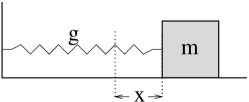
Fig. 1. : Simple harmonic oscillator

In this simple example the Lagrangian is given by

$$L = \frac{1}{2}m\dot{x}^{2}-\frac{1}{2}gx^{2},$$ (1)

and from the Euler-Lagrange equations the nonperturbative result follows as:

$$x(t) = A\,{\rm Sin}(wt),\hskip 56.9055ptw=\sqrt{\frac{g}{m}}.$$ (2)

One might express this result as a power series in the coupling strength

$$x(t) = A\biggl{[}wt-\frac{(wt)^{3}}{3!}+\frac{(wt)^{5}}{5!}+\cdots\biggr{]}.$$ (3)

As this expansion shows a perturbative truncation of the above series can not produce a bound state. In other words, in order to be able to obtain a bound state result one must sum the interactions to all orders.

The situation in field theory is similar. Bound states in field theory are identified by the pole of Green’s function.

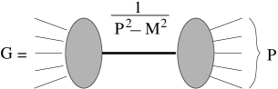
Fig. 2. : Bound state mass is determined by the pole of Green’s function

In general the Green’s function can be expanded in powers of the coupling strength. The question is then: Can we make a truncation in the perturbation series at order $g^{2n}$ and still obtain a bound state ?

$$G\stackrel{{\scriptstyle?}}{{\simeq}}G_{0}+g^{2}G_{1}+g^{4}G_{2}+\cdots+g^{2i}\framebox{$G_{i}$}+\cdots+g^{2n}G_{n}.$$ (4)

Since this is a finite series, the bound state singularity could only come from individual terms

$$\framebox{$G_{i}$}\,\propto\,\frac{1}{P^{2}-M^{2}}\,\,\,?$$ (5)

However this possibility leads to a contradiction since it implies that the dynamics of the bound state is independent of $g$, since $g$ comes only as an overall factor in front of an individual term $G_{i}$. The case where more than one term is singular leads to the same contradiction. Therefore individual $G_{i}$’s must be nonsingular, and bound state singularity must come from an infinite summation of the perturbation series. Situation is similar to the expansion

$$\frac{1}{1-x}=1+x+x^{2}+x^{3}+\cdots,$$ (6)

where the singularity of the left hand side can not be obtained by a finite truncation of the right side. Therefore bound states are always fully nonperturbative.

With the discovery of quantum chromo-dynamics (QCD) nonperturbative calculations in field theory have become even more essential. It is known that the building blocks of matter, quarks and gluons, only exist in bound states. Therefore any reaction that involves quarks will necessarily involve bound states in the initial and/or final states. This implies that even at high momentum transfers, where QCD is perturbative, formation of quarks into a bound state necessitates a nonperturbative treatment. Therefore it is essential to develop new methods for doing nonperturbative calculations in field theory.

The plan of this lecture is as follows. In the following section a review of nonperturbative methods in field theory will be given. Later in Sections 3 and 4 the Feynman-Schwinger representation will be introduced through examples. In particular the emphasis will be on comparing various nonperturbative results obtained by different methods. It will be shown with examples that nonperturbative calculations are interesting and exact nonperturbative results could significantly differ from those obtained by approximate nonperturbative methods. In the last section simple perturbation theory results will be derived using the FSR approach.

2 Nonperturbative methods

Nonperturbative calculations can be divided into two general categories. These are i) Integral equations, and ii) Path integrals. In the following two subsections these approaches will be briefly discussed

2.1 Integral Equations

Integral equations have been used for a long time to sum interactions to all orders with various approximations. [1, 2, 3, 4, 5] In general a complete solution of field theory to all orders can be provided by an infinite set of integral equations relating vertices and propagators of the theory to each other. However solving an infinite set of equations is beyond our reach and usually integral equations are truncated by various assumptions about the interaction kernels and vertices. The most commonly used integral equations are those that deal with 1, and 2-body problems. Here we give 2 examples for the 2-body bound state problem. The first example is the Bethe-Salpeter equation in the ladder approximation. [1]

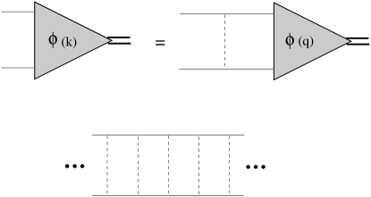
Fig. 3. : Bethe-Salpeter equation in the ladder approximation sums only ladder type diagrams

In the ladder approximation the Bethe-Salpeter equation sums ladder diagrams to all orders (Fig. 3). Self energies vertex corrections and crossed ladder exchanges are left out in this approximation. For the simple case of scalar particles, The vertex function $\Phi_{P}(k)$ determining the structure of bound state satisfies an integral equation. For the simple case of scalar particles bound state equation can be written as

$$\Phi_{P}(k) = ig^{2}\biggl{\lmoustache}\,\frac{d^{4}q}{(2\pi)^{4}}\,G(q-k)\,\frac{\Phi_{P}(q)}{[q^{2}-M^{2}][(P-q)^{2}-m^{2}]},$$ (7)

where $G(q-k)$ is the interaction kernel. This equation could be solved using numerical methods to find the bound state mass $P$ and the vertex function $\Phi_{P}(k)$. The vertex function is similar to the quantum mechanical wave function. In principle it contains all information about the bound state. A serious deficiency of the ladder approximation is that it does not have the correct one body limit when one of the particles is infinitely heavy. [3] This is due to the fact that the ladder approximation ignores the crossed ladder type exchanges between the particles. As it will be shown by explicit examples in this article the crossed ladder exchanges play a crucial role in obtaining the correct result not only in the 2-body problem but also in the calculation of self energies for the 1-body propagators.

The problem of 1-body limit when one of the particles is infinitely heavy is solved by the Gross equation (Fig. 4). [3] In the Gross equation the heavier constituent is constraint to its physical mass shell ($q^{2}=M^{2}$)

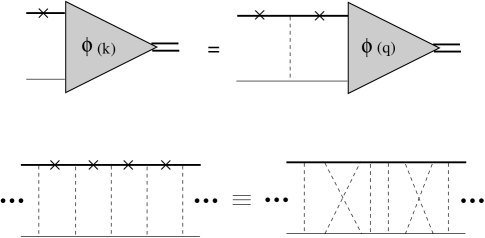
Fig. 4. : In the limit of infinitely heavy-light systems Gross equation effectively sums all ladder and crossed ladder diagrams.

Putting the heavier constituent on its mass shell and summing only ladder diagrams effectively is equivalent to summing all ladder and crossed ladder diagrams. When the heavy particle is constraint to its mass shell, the bound state equation takes the following form

$$\Phi_{P}(\hat{k}) = g^{2}\biggl{\lmoustache}\,\frac{d^{3}q}{(2\pi)^{3}\,2E_{q}}\,G(\hat{q}-\hat{k})\,\frac{\Phi_{P}(\hat{q})}{[(P-\hat{q})^{2}-m^{2}]}.$$ (8)

When bound state of equal (or close) mass particles are under consideration the Gross equation can be symmetrized by picking up the mass pole contribution of both particles in different channels. Gross equation is a manifestly covariant relativistic equation, and in the nonrelativistic limit Schroedinger equation is recovered. In the literature this equation has been successfully used to analyze relativistic bound states.

Some general comments on integral equations are as follows: There are a number of useful features of integral equations. Integral equations are a natural extension of nonrelativistic quantum mechanics to field theory. They are a practical tool for modeling and doing simple calculations using the tools of field theory. Because of their similarity to Schroedinger equation in quantum mechanics, integral equations in field theory provide an intuitively clear picture of physics. Furthermore the numerical cost of solving integral equations is negligibly small compared to methods such as path integrals (to be discussed in the next section). The last important advantage of integral equations is the fact that they can be solved in Minkowski metric. The only other alternative to integral equations, path integrals, make use of the Euclidean metric which limits their applicability. This is an important technical problem -particularly for calculations of scattering reactions, form factors and decays- since physical particles live in the timelike region.

On the other hand integral equations have some drawbacks. The first problem is that they are not exact. Without knowing the exact result it is not possible to claim that integral equations are even a good approximation to the full theory. The second problem is that integral equations in general do not respect the symmetries of the underlying Lagrangian. Except for very special approximations, integral equations are not gauge invariant. Therefore a more rigorous and systematic approach is needed. This is where path integrals play a significant role. In the next section we introduce the method of path integrals in quantum mechanics and field theory.

2.2 Path Integrals

Path integrals provide a systematic method for summing interactions to all orders. First we begin by giving path integral expressions for quantum mechanics. The matrix element for a transition from an initial state $|q_{i},t_{i}\rangle$ to a final state $|q_{f},t_{f}\rangle$ is given by

$$\langle q_{f},t_{f}|q_{i},t_{i}\rangle_{H} \equiv \langle q_{f},t_{f}|\,e^{-iH\,(t_{f}-t_{i})}|q_{i},t_{i}\rangle_{S},$$ (9)

$$\langle q_{f},t_{f}|\,e^{-iH\,(t_{f}-t_{i})}|q_{i},t_{i}\rangle = \biggl{\lmoustache}\,{\cal D}q\,e^{\,i\bigl{\lmoustache}_{t_{i}}^{t_{f}}L(q,\dot{q},t)\,dt/\hbar},$$ (10)

where subscripts H, and S refer to Heisenberg and Schroedinger states. In this path integral expression all trajectories contribute to the final result with equal weight.

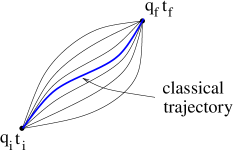
Fig. 5. : In quantum mechanics all paths contribute.

Classical limit can be readily obtained by letting $\hbar\rightarrow 0$. In this limit small variations in the action will lead to large oscillations and the dominant contribution will come from those trajectories that minimize the action:

$$\delta S = \delta\biggl{\lmoustache}_{q_{i}}^{q_{f}}\,L[q,\dot{q},t]\,dt=0.$$ (11)

The minimization of the action leads to Euler-Lagrange equations of classical mechanics:

$$\frac{d}{dt}\biggl{[}\frac{\partial L}{\partial\dot{q}}\biggr{]}-\frac{\partial L}{\partial q} = 0.$$ (12)

Keeping the field theory applications in mind we consider the time ordered products of operators. The time ordered product of operators can also be expressed in the form of a path integral:

$$\langle q_{f},t_{f}|T(\hat{q}(t_{1})\hat{q}(t_{2})\cdots\hat{q}(t_{n})|q_{i},t_{i}\rangle = \biggl{\lmoustache}{\cal D}q\,q(t_{1})\,q(t_{2})\cdots q(t_{n})\,{\rm exp}\biggl{[}i\int_{t_{i}}^{t_{f}}dt\,L(q,\dot{q})\biggr{]}.$$

In field theory applications the ground state expectation values of time ordered products are particularly needed. In order to show how the ground state expectation value can be obtain let us introduce a complete set of energy eigenstates into the 2-point Green’s function

$$\langle q_{f},t|T[\hat{q}(t_{1})\hat{q}(t_{2})]|q_{i},-t\rangle = \sum_{n,m=0}^{\infty}\langle q_{f},t_{f}|n\rangle\langle n|T[\hat{q}(t_{1})\hat{q}(t_{2})]|m\rangle\langle m|q_{i},t_{i}\rangle.$$ (13)

Noting that

$$\langle q,t|n\rangle = \psi_{n}(q)e^{-iE_{n}t},$$ (14)

one obtains

$$\langle q_{f},t|T[\hat{q}(t_{1})\hat{q}(t_{2})]|q_{i},-t\rangle = \sum_{n,m=0}^{\infty}{\rm e}^{-i(E_{n}+E_{m})t}\psi_{n}(q_{f})\psi_{m}(q_{i})\langle n|T[\hat{q}(t_{1})\hat{q}(t_{2})]|m\rangle.$$

As $t\rightarrow-i\infty$ the ground state $(n=0)$ will give the dominant contribution,

$$\lim_{t\rightarrow\infty}\langle q_{f},t|T[\hat{q}(t_{1})\hat{q}(t_{2})]|q_{i},-t\rangle \simeq \underbrace{{\rm e}^{-2E_{0}t}\psi_{0}(q_{f})\psi_{0}(q_{i})}_{\langle q_{f},t|q_{i},-t\rangle}\langle 0|T[\hat{q}(t_{1})\hat{q}(t_{2})]|0\rangle.$$ (15)

Therefore the ground state expectation value is obtained as

$$\langle 0|T[\hat{q}(t_{1})\hat{q}(t_{2})]|0\rangle = \frac{\langle q_{f},\infty|T[\hat{q}(t_{1})\hat{q}(t_{2})]|q_{i},-\infty\rangle}{\langle q_{f},\infty|q_{i},-\infty\rangle}.$$ (16)

In general the ground state expectation value of the time ordered products of an arbitrary number of operators can be written as

$$\langle 0|T[\hat{q}(t_{1})\hat{q}(t_{2})\cdots\hat{q}(t_{n})]|0\rangle = \frac{\biggl{\lmoustache}{\cal D}q\,q(t_{1})\,q(t_{2})\cdots q(t_{n})\,{\rm exp}\biggl{[}i\int_{-\infty}^{\infty}dt\,L(q,\dot{q})\biggr{]}}{\biggl{\lmoustache}{\cal D}q\,{\rm exp}\biggl{[}i\int_{-\infty}^{\infty}dt\,L(q,\dot{q})\biggr{]}}.$$

In going from quantum mechanics to quantum field theory we recognize that a field is an infinite array of coordinates, such as an infinite array of coupled oscillators, and particles are associated with the normal modes of oscillators. Therefore the quantum mechanical derivation can be generalized by replacing

$$q(t)\rightarrow\phi({\bf x}_{1},t),\phi({\bf x}_{2},t),\cdots,\phi({\bf x}_{n},t),\cdots,$$ (17)

where $\phi({\bf x}_{i},t)$ is the displacement of the oscillator at $x_{i}$.

Fig. 6. : Field as the coordinates of an infinite array of coupled oscillators

The generalized path integral in terms of fields is given by:

$$\langle\phi({\bf x},t_{f})|\,{\rm exp}\biggl{[}-iH\,(t_{f}-t_{i})\biggr{]}|\phi({\bf x},t_{i})\rangle = \biggl{\lmoustache}\,{\cal D}\phi\,{\rm exp}\biggl{[}\,i\int_{t_{i}}^{t_{f}}\,d^{4}xL\,\biggr{]},$$ (18)

where

$${\cal D}\phi=\Pi_{i}d\Phi(x_{i}),$$ (19)

represents a sum over all possible field configurations. The step of going from particle trajectories $q(t)$ to fields $\phi({\bf x},t)$ dramatically increases the dimensionality of the problem. While quantum mechanical path integral sums all possible trajectories (line configuration), field theoretical path integral sums all possible field configurations (volume configuration).

The Green’s function in field theory is given by the path integral expression:

$$\langle 0|T[\phi(x_{1})\phi(x_{2})\cdots\phi(x_{n})]|0\rangle = \frac{\biggl{\lmoustache}[{\cal D}\phi]\,\phi(x_{1})\,\phi(t_{2})\cdots\phi(x_{n})\,{\rm exp}\biggl{[}i\int d^{4}x\,L(x)\biggr{]}}{\biggl{\lmoustache}[{\cal D}\phi]\,{\rm exp}\biggl{[}i\int d^{4}x\,L(x)\biggr{]}}.$$

This result can be obtained from a generating function

$$\langle 0|T(\phi(x_{1})\phi(x_{2})\cdots\phi(x_{n})|0\rangle = (-i)^{n}\frac{\delta^{n}Z[J(x)]}{\delta J(x_{1})\delta J(x_{2})\cdots\delta J(x_{n})}\Bigg{|}_{J=0},$$ (20)

where

$$Z[J(x)] = \biggl{\lmoustache}[{\cal D}\phi]\,{\rm exp}\biggl{[}i\int d^{4}x\,[L(x)+J(x)\phi(x)]\biggr{]}.$$ (21)

While path integrals provide a compact expression for the exact nonperturbative result for propagators, evaluation of the path integral is a nontrivial task. In general, field theoretical path integrals must be evaluated by numerical integration methods, such as Monte-Carlo integration. The best known numerical integration method is lattice gauge theory. [6] Lattice gauge theory involves a discretization of space-time.

Fig. 7. : In lattice gauge theory space-time is discretized within a finite box.

In a discretized lattice particles can be located on the discrete lattice sites and exchange fields are represented by links between the sites. After discretization the path integral can be performed essentially by a brute force method. Particularly for QCD lattice gauge theory is currently the only method that can produce nonperturbative results starting directly from the QCD Lagrangian. However lattice calculations are not without drawbacks. Discretization of space-time by a cubic lattice violates rotational symmetry. In addition the cost of computations critically depend on the size of the lattice. Because of this limitation complex applications such as calculation of form factors or scattering reactions are beyond the reach of current lattice applications. Finally, matter loops are not accounted for (quenched approximation) in most lattice calculations due to high cost.

In the next section we present a more efficient method of performing path integrals in field theory for simple scalar interactions. This method is known as Feynman-Schwinger representation(FSR). [7, 8, 9, 10, 11, 12, 13, 14, 15] Through applications of the FSR, the importantance of exact nonperturbative calculations will be shown with explicit examples.

3 Feynman-Schwinger representation approach

The basic idea in the FSR approach is to transform the field theoretical path integral such that a quantum mechanical path integral in terms of particle trajectories is obtained. In this section we consider application of the FSR technique to scalar QED. The Minkowski metric expression for the scalar QED Lagrangian in Stueckelberg form is given by

$${\cal L}_{SQED} = -m^{2}\chi^{2}-\frac{1}{4}F^{2}+\frac{1}{2}\mu^{2}A^{2}-\lambda\frac{1}{2}(\partial A)^{2}+(\partial_{\mu}-ieA_{\mu})\chi^{*}(\partial^{\mu}+ieA^{\mu})\chi,$$

where $A$ represents the gauge field of mass $\mu$, and $\chi$ is the charged field of mass $m$. The presence of a mass term for the exchange field breaks the gauge invariance. Here the mass term was introduced in order to avoid infrared singularities when application to 0+1 dimension is considered later in the next section. For dimensions larger than n=2 the infrared singularity does not exist and therefore the limit $\mu\rightarrow~{}0$ can be safely taken to insure gauge invariance.

The path integral is to be performed in Euclidean metric. Therefore we perform a Wick rotation:

$${\rm exp}\biggl{[}i\int d^{4}x\,{\cal L}_{M}\biggr{]}\longrightarrow{\rm exp}\biggl{[}-\int d^{4}x\,{\cal L}_{E}\biggr{]}.$$

The Wick rotation for coordinates is obtained by

$$x_{0} \rightarrow -ix_{0}$$ (22)

$$\partial_{0}=\frac{\partial}{\partial x_{0}} \rightarrow i\partial_{0}.$$ (23)

The transformation of field $A$ under Wick rotation is found by noting that under a gauge transformation:

$$A_{\mu} \rightarrow A_{\mu}+\partial_{\mu}\Lambda.$$ (24)

Then, under a Wick rotation:

$$A_{0} \rightarrow iA_{0}.$$ (25)

The Wick rotated Lagrangian for SQED is given by:

$${\cal L}_{SQED} = \chi^{*}\biggl{[}m^{2}-\partial^{2}-2ieA\partial-ie\partial A+e^{2}A^{2}\biggr{]}\chi+{\cal L}_{A}.$$ (26)

The exchange field part of the Lagrangian is given by

$${\cal L}_{A} \equiv \frac{1}{2}A_{\mu}(\mu^{2}g_{\mu\nu}-\lambda\partial_{\mu}\partial_{\nu})A_{\nu}+\frac{1}{4}F^{2},$$ (27)

$$= \frac{1}{2}A_{\mu}[(\mu^{2}-\Box)g_{\mu\nu}+(1-\lambda)\partial_{\mu}\partial_{\nu}]A_{\nu}.$$ (28)

We employ the Feynman gauge $\lambda=1$ which yields

$${\cal L}_{A} = \frac{1}{2}A_{\nu}(\mu^{2}-\Box)A_{\nu}.$$ (29)

The two-body Green’s function for the transition from an initial state $\Phi_{i}$ to final state $\Phi_{f}$ is given by

$$G(y,\bar{y}|x,\bar{x})=N\int{\cal D}\chi^{*}\int{\cal D}\chi\int{\cal D}A\,\,\Phi^{*}_{f}\Phi_{i}\,e^{-S_{E}},$$ (30)

where

$$S_{E}=\int d^{4}x\,\,{\cal L}_{SQED},$$ (31)

and a gauge invariant 2-body state $\Phi$ is defined by

$$\Phi(x,\bar{x}) = \chi^{*}(x)U(x,\bar{x})\chi(\bar{x}).$$ (32)

The gauge link $U(x,y)$ which insures gauge invariance of bilinear product of fields is defined by

$$U(x,y)\equiv{\rm exp}\left[-ie\int_{x}^{y}dz\,A(z)\right].$$ (33)

One can easily see that under a local gauge transformation

$$\chi(x) \rightarrow {\rm e}^{ie\Lambda(x)}\chi(x)$$ (34)

$$A_{\mu}(x) \rightarrow A_{\mu}(x)+\partial_{\mu}\Lambda(x),$$ (35)

$\Phi_{i}(x,\bar{x})$ remains gauge invariant

$$\Phi(x,\bar{x}) \rightarrow {\rm exp}\biggl{[}\underbrace{-ie\Lambda(x)+ie\Lambda(\bar{x})-ie\biggl{\lmoustache}_{x}^{\bar{x}}dz_{\mu}\,\partial_{\mu}\Lambda}_{0}\biggr{]}\chi^{*}(x)U(x,\bar{x})\chi(\bar{x})$$ (36)

$$= \Phi(x,\bar{x}).$$ (37)

Performing path integrals over $\chi$ and $\chi^{*}$ fields in Eq. 30 one finds

$$G(y,\bar{y}|x,\bar{x}) = N\bigg{\lmoustache}{\cal D}A\,({\rm det}S)\,\,U(x,\bar{x})U^{*}(y,\bar{y})S(x,y)S(\bar{x},\bar{y})\,e^{-S[A]},$$ (38)

where the interacting 1-body propagator $S(x,y)$ is defined by

$$S(x,y) \equiv \langle y\,|\,\frac{1}{m^{2}+H(\hat{z},\hat{p})}\,|\,x\rangle,$$ (39)

$$H(\hat{z},\hat{p}) \equiv (\hat{p}+ieA(\hat{z}))^{2}.$$ (40)

The Green’s function Eq. 38 in principle includes contributions coming from all possible interactions. The determinant in Eq. 38 accounts for matter loops and in the quenched approximation it is set equal to one (${\rm det}S\rightarrow 1$).

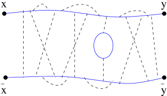
Fig. 8. : Various interactions in presence of a matter loop

Analytical calculation of the path integral over gauge field $A$ in Eq. 38 seems difficult due to nontrivial $A$ dependence in $S(x,y)$. In more complicated theories such as QCD integration of gauge field integral, as far as we know, is not analytically doable. Therefore, in QCD, the only option is to do the gauge field path integral by using a brute force method on a discretized space-time lattice. However for the simple scalar QED interaction under consideration it is in fact possible to go further and eliminate the path integral over field A. In order to be able to carry out the remaining path integral over the exchange field $A$ it is desirable to represent the interacting propagator in the form of an exponential. This can be achieved by using a Feynman representation for the interacting propagator. The first step involves the exponentiation of the denominator in Eq. 39:

$$S(x,y) = \int_{0}^{\infty}ds\,\,\,e^{-sm^{2}}\,\langle y\,|\,{\rm exp}[-sH]\,|\,x\rangle,$$ (41)

This expression is similar to a quantum mechanical propagator where $s=it$, and H is a covariant Hamiltonian in terms of 4-vector momentum and coordinates. It is known that one can use a path integral representation for quantum mechanical propagators. A covariant Lagrangian can easily be obtained from the Hamiltonian

$$H(\hat{z},\hat{p})=(\hat{p}+ieA(\hat{z}))^{2},\,\,\Longrightarrow\,\,L(z,\dot{z})=\frac{\dot{z}^{2}}{4}-ie\dot{z}A(z).$$ (42)

Using this Lagrangian a path integral representation for the interacting propagator can be constructed

$$S(x,y) = \bigg{\lmoustache}_{0}^{\infty}ds\,\bigg{\lmoustache}\,{\cal D}z\,\,{\rm exp}\biggl{[}-sm^{2}-\frac{1}{4}\int_{0}^{s}d\tau\,\dot{z}^{2}(\tau)-ie\int_{0}^{s}d\tau\,\dot{z}A(z(\tau))\,\,\biggr{]},$$ (43)

where the boundary conditions are given by $z(0)=x$, $z(s)=y$. This representation allows one to perform the remaining path integral over the exchange field $A$. The final result for the two-body propagator involves a quantum mechanical path integral that sums up contributions coming from all possible trajectories of particles

$$G = -\bigg{\lmoustache}_{0}^{\infty}ds\,\,\bigg{\lmoustache}_{0}^{\infty}d\bar{s}\,\,\bigg{\lmoustache}\,({\cal D}z)_{xy}\,\bigg{\lmoustache}\,({\cal D}\bar{z})_{\bar{x}\bar{y}}\,\,e^{-K[z,s]-K[\bar{z},\bar{s}]}\langle W(C)\rangle,$$ (44)

where the kinetic term is defined by

$$K[z,s] = m^{2}s+\frac{1}{4s}\int_{0}^{1}d\tau\,\dot{z}^{2}(\tau),$$ (45)

and the Wilson loop average $\langle W(C)\rangle$ is given by

$$\langle W(C)\rangle \equiv \int{\cal D}A\,{\rm exp}\biggl{[}-ie\oint_{C}dz\,A(z)-\frac{1}{2}\int d^{4}z\,A(z)(\mu^{2}-\partial^{2})A(z)\biggr{]},$$ (46)

where the contour of integration $C$ (Fig. 9) follows a clockwise trajectory $x\rightarrow y\rightarrow\bar{y}\rightarrow\bar{x}\rightarrow x$ as parameters $\tau$, and $\bar{\tau}$ are varied from 0 to $1$.

Fig. 9. : Wilson loop.

The $A$ integration in the definition of the Wilson loop average is of standard gaussian form and can be easily performed to obtain

$$\langle W(C)\rangle = {\rm exp}\,\biggl{[}-\frac{e^{2}}{2}\int_{C}\,dz_{\mu}\,\int_{C}\,d\bar{z}_{\nu}\,\Delta_{\mu\nu}(z-\bar{z},\mu)\biggl{]},$$ (47)

$$\Delta_{\mu\nu}(x,\mu) = g_{\mu\nu}\bigg{\lmoustache}\frac{d^{4}p}{(2\pi)^{4}}\frac{e^{ipx}}{p^{2}+\mu^{2}},$$ (48)

The self energy and the exchange interaction contributions, which are embedded in expression 47, have different signs. This follows from the fact that particles forming the two body bound state carry opposite charges. By the result given in Eq. 44 and Eq. 47 path integration expression involving fields has been transformed into a path integral representation involving trajectories of particles. The bound state spectrum can be determined from the spectral decomposition of the two body Green’s function

$$G(T)=\sum_{n=0}^{\infty}c_{n}e^{-m_{n}T},$$ (49)

where T is defined as the average time between the initial and final states

$$T\equiv\frac{1}{2}(y_{4}+\bar{y}_{4}-x_{4}-\bar{x}_{4}).$$ (50)

In the limit of large $T$, the ground state mass is given by

$$m_{0}=\lim_{T\rightarrow\infty}-\frac{d}{dT}{\rm ln}[G(T)]=\frac{\int{\cal D}ZS^{\prime}[Z]e^{-S[Z]}}{\int{\cal D}Ze^{-S[Z]}}.$$ (51)

3.1 Application to 0+1 dimensions

Massive scalar QED in 0+1 dimension is a simple interaction that enables one to obtain a fully analytical result for the dressed and bound state masses within the FSR approach. In this section we compare the self energy result obtained by approximate methods with the full result obtained from the Feynman-Schwinger representation. In 0 space + 1 time dimension there is no continuum spectrum, and only bound states exist.

In general Wilson loop average depends on the trajectory of particles:

$$\langle W(C)\rangle = {\rm exp}\,\biggl{[}-\frac{e^{2}}{2}\int_{C}\,dz\,\int_{C}\,d\bar{z}\,\Delta(z-\bar{z},\mu)\biggl{]}.$$ (52)

In 0+1 dimensions Wilson loop integral is essentially a line integral and all trajectories contribute equally. Therefore in 0+1 dimension Wilson loop average does not depend on the shape of trajectory

$${\langle W(C)\rangle} = {\rm exp}\,\biggl{[}-\frac{e^{2}}{2}\int_{0}^{T}\,dz\,\int_{0}^{T}\,d\bar{z}\,\Delta(z-\bar{z},\mu)\biggl{]}.$$ (53)

Notice that in 0+1d all trajectories lie on a straight line. Possible variations can only come from those trajectories which fold onto themselves. However the contribution of the folded sections of trajectories identically vanish. In addition, contribution of matter loops to the Wilson loop average is identically zero. The typical loop contribution in 1-dimension can be written as

$$\int_{0}^{T}dz\,\biggl{(}\int_{z_{i}}^{z_{f}}dz^{\prime}+\int_{z_{f}}^{z_{i}}dz^{\prime}\biggr{)}\Delta(z-z^{\prime}) = 0.$$ (54)

The vanishing of matter loop contribution implies that the quenched calculations give exact results. Therefore massive SQED in 0+1 dimension is a remarkably simple example where we can compare exact analytic solutions of field theory with various approximate nonperturbative methods. Furthermore, analytical results in 0+1d provide a test case for the numerical routines which are used in higher dimensions.

In 0+1d the interaction kernel $\Delta(z-\bar{z},\mu)$ is given by

$$\Delta(z-\bar{z},\mu) = \frac{e^{-\mu|z-\bar{z}|}}{2\mu}.$$ (55)

Using this kernel the Wilson loop average Eq. 53 is calculated exactly:

$${\langle W(C)\rangle} = {\rm exp}\,\biggl{[}-\frac{e^{2}T}{2\mu^{2}}\biggl{(}1-\frac{1-e^{-\mu T}}{\mu T}\biggr{)}\biggr{]}.$$ (56)

Remaining integrals over $ds$ and ${\cal D}z$ in Eq. 44 provide the free particle exponential fall of $e^{-mT}$ at large times. Therefore the spectrum of the Green’s function can be trivially calculated using Eqs. 44, 51, and 56. Exact analytic FSR results for bound state masses are as follows:

$${\rm 1-body:}\,\,\,\,\,\,M_{1}=m+\frac{e^{2}}{2\mu},$$ (57)

$${\rm 2-body:}\,\,\,\,\,\,M_{2}=2m,$$ (58)

$${\rm n-body:}\,\,\,\,\,\,M_{n}=n\,m-n\,(n-2)\,\frac{e^{2}}{2\mu}.$$ (59)

Bound state mass results given above include the self energy contributions. The n-body result shows that for any given coupling strength $e$, there is an upper limit in particle number $n$ beyond which results become unstable. Dynamics of the two body bound state mass generation is similar to pion mass generation. Self energies of particles exactly cancel the binding energy to produce a bound state mass that is proportional to the current masses

$$(m+\frac{e^{2}}{2\mu})+(m+\frac{e^{2}}{2\mu})-\frac{e^{2}}{\mu}=2m.$$ (60)

Exact massive SQED results share some common features with QCD in 1+1 d [16],

• $\mu\rightarrow 0\Longrightarrow M_{1}\rightarrow\infty$, where $\mu$ plays the role of an infrared cut-off.

• 2-body bound state mass $M_{2}$ is independent of $\mu$.

• When “cut-off” $\mu\rightarrow 0\Longrightarrow$ no bound states for $n>2$.

• When current masses vanishes $m\rightarrow 0\Longrightarrow M_{2}=0$ “chiral limit”

This toy model provides a possible test case also for the lattice gauge theory calculations.

3.2 Comparison of the exact FSR results with approximate nonperturbative methods

In this section we take a closer look at 1-body mass pole calculations. Popular methods frequently used in finding the dressed mass of a particle is to do a simple bubble summation or solve the 1-body Dyson-Schwinger equation in rainbow approximation. It is interesting to compare results given by the bubble summation and the Dyson-Schwinger with the exact FSR result. Below we first give a quick overview of how dressed masses can be obtained in bubble summation and the Dyson-Schwinger equation approaches.

Fig. 10. : Various interactions included in each approach are shown.

The simple bubble summation involves a summation of all bubble diagrams (Fig. 10) to all orders. The dressed propagator is given by

$$\Delta_{d}(p) = \frac{1}{p^{2}+m^{2}+\Sigma(p)}.$$ (61)

The dressed mass M is determined from the self energy using

$$M=\sqrt{m^{2}+\Sigma(iM)}.$$ (62)

The self energy for the simple bubble sum is given by

$$\Sigma(p) = -e^{2}\bigg{\lmoustache}_{-\infty}^{\infty}\frac{dk}{2\pi}\frac{1}{(k^{2}+\mu^{2})}\bigg{\{}\frac{(2p-k)^{2}}{[(p-k)^{2}+m^{2}]}-1\bigg{\}}.$$ (63)

The self energy integral in this case is trivial and can be performed analytically, and the dressed mass is determined from Eq. 62

The rainbow Dyson-Schwinger equation sums more diagrams than the simple bubble summation (Fig. 10). The self energy of the rainbow Dyson-Schwinger equation involves a momentum dependent mass.

$$\Sigma(p) = -e^{2}\bigg{\lmoustache}_{-\infty}^{\infty}\frac{dk}{2\pi}\frac{1}{(k^{2}+\mu^{2})}\bigg{\{}\frac{(2p-k)^{2}}{[(p-k)^{2}+\underbrace{m^{2}+\Sigma(k)}]}-1\bigg{\}}.$$ (64)

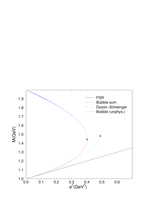
Fig. 11. : The function $M(e^{2})$ calculated by the FSR approach, the Dyson-Schwinger equation in the rainbow approximation, and the bubble summation for values of $m=\mu=1$ GeV. While the exact result is always real, the rainbow DSE and the bubble summation results become complex beyond a critical coupling.

In this case the self energy is nontrivial and it must be determined by a numerical solution of Eq. 64. The dressed mass is determined by the logarithmic derivative of the dressed propagator in coordinate space

$$M = -\lim_{T\rightarrow\infty}\frac{d}{dT}\,\,{\rm log}[\,\Delta_{d}(t)\,].$$ (65)

The type of diagrams summed by each method is shown Fig. 10. Note that the matter loops do not give any contribution as explained earlier. Results obtained by these three methods are shown in Fig. 11. It is interesting to note that the simple bubble summation and the rainbow Dyson-Schwinger results display similar behavior. While the exact result provided by the FSR linearly increases for all coupling strengths, both the simple bubble summation and the rainbow Dyson-Schwinger results come to a critical point beyond which solutions for the dressed masses become complex. This example very clearly shows that conclusions about the mass poles of propagators based on approximate methods such as rainbow Dyson-Schwinger equation can be misleading.

Fig. 12. : As a test of the numerical methods the numerical Monte-Carlo result for 1-body dressed mass in SQED is compared with the analytical result.

The simplicity of massive SQED in 0+1d also provides an excellent opportunity to test the numerical Monte-Carlo integration methods which are normally needed at higher dimensions. Therefore as a test of the numerical methods used for the remainder of applications in this work, we demonstrate in Fig. 12 that the numerical Monte-Carlo results for 1-body dressed mass in SQED correctly reproduce the analytical result. In Fig. 12 the time dependence of the dressed mass given by Eq. 51 is shown. Parameters used for this plot are $\mu=0.15$ Gev, and $e=0.15$ $GeV^{1.5}$.

In the next section we consider the application of the FSR approach to scalar $\chi^{2}\phi$ interaction

4 Scalar $\chi^{2}\phi$ interaction with the FSR approach

We consider the theory of charged scalar particles $\chi$ of mass $m$ interacting through the exchange of a neutral scalar particle $\phi$ of mass $\mu$. The Euclidean Lagrangian for this theory is given by

$${\cal L} = \chi^{*}\bigl{[}m^{2}-\partial^{2}+g\phi\bigr{]}\chi+\frac{1}{2}\,\phi(\mu^{2}-\partial^{2})\phi.$$ (66)

The 2-body propagator for the transition from the initial state $\Phi_{i}=\chi^{*}(x)\chi(\bar{x})$ to final state $\Phi_{f}=\chi^{*}(y)\chi(\bar{y})$ is given by

$$G(y,\bar{y}|x,\bar{x})=N\bigg{\lmoustache}{\cal D}\chi^{*}\bigg{\lmoustache}{\cal D}\chi\bigg{\lmoustache}{\cal D}A\,\,\,\Phi^{*}_{f}\,\Phi_{i}\,\,{\rm exp}\biggl{[}-\int d^{4}x\,{\cal L}\biggr{]}.$$ (67)

After the usual integration of matter fields is done the Green’s function reduces to

$$G(y,\bar{y}|x,\bar{x}) = N\bigg{\lmoustache}{\cal D}\phi\,({\rm det}S)\,\,S(x,y)S(\bar{x},\bar{y})\,e^{-S[\phi]}.$$ (68)

As in the case of scalar QED we employ the quenched approximation: ${\rm det}S\rightarrow 1$. The interacting propagator $S(x,y)$ is defined as

$$S(x,y) \equiv \langle y\,|\,\frac{1}{m^{2}+H(\hat{z},\hat{p})}\,|\,x\rangle$$ (69)

$$H(\hat{z},\hat{p}) \equiv \hat{p}^{2}-g\phi(\hat{z}).$$ (70)

We exponentiate the denominator by introducing an $s$ integration along the imaginary axis with an $\epsilon$ prescription

$$S(x,y) = \int_{0}^{i\infty}ds\,\,\,e^{-s(m^{2}+i\epsilon)}\,\langle y\,|\,{\rm exp}[-sH]\,|\,x\rangle.$$ (71)

This representation should be compared with the representation used earlier in SQED Eq. 41. Here the integration is done along the imaginary axis because $H$ is not positive definite. Again a quantum mechanical path integral representation can be constructed by recognizing that Lagrangian corresponding to $H$ Eq. 70 is given by

$$L(z,\dot{z})=\frac{\dot{z}^{2}}{4}+g\phi(z).$$ (72)

The path integral representation for the interacting propagator is

$$S(x,y) = -i\bigg{\lmoustache}_{0}^{\infty}ds\,\bigg{\lmoustache}\,{\cal D}z\,\,{\rm exp}\biggl{[}is(m^{2}+i\epsilon)-\frac{i}{4}\int_{0}^{s}d\tau\,\dot{z}^{2}(\tau)+ig\int_{0}^{s}d\tau\,\phi(z(\tau))\,\,\biggr{]}.$$

This representation allows the elimination of the integral over exchange field $\phi$. The 2-body propagator reduces to

$$G = -\bigg{\lmoustache}_{0}^{\infty}ds\,\,\bigg{\lmoustache}_{0}^{\infty}d\bar{s}\,\,\bigg{\lmoustache}\,({\cal D}z)_{xy}\,\bigg{\lmoustache}\,({\cal D}\bar{z})_{\bar{x}\bar{y}}\,\,e^{iK[z,s]+iK[\bar{z},\bar{s}]}I_{\phi},$$ (73)

where mass and kinetic term is given by

$$K[z,s] = (m^{2}+i\epsilon)s-\frac{1}{4s}\int_{0}^{1}d\tau\,\dot{z}^{2}(\tau).$$ (74)

The field integration $I_{\phi}$ is a standard gaussian integration

$$I_{\phi} \equiv \biggl{\lmoustache}{\cal D}\phi\,{\rm exp}\biggl{[}+ig\biggl{(}\int_{0}^{s}d\tau\,\phi(z(\tau))+\int_{0}^{\bar{s}}d\bar{\tau}\,\phi(\bar{z}(\bar{\tau}))\biggr{)}-S[\phi]\biggr{]}$$ (75)

$$\equiv {\rm exp}\biggl{(}-V_{0}[z,s]-2\,V_{12}[z,\bar{z},s,\bar{s}]-V_{0}[\bar{z},\bar{s}]\biggr{)},$$ (76)

where $V_{0}$ and $V_{12}$ (self and exchange energy contributions in Fig. 13) are defined by

$$V_{0}[z,s] = \frac{g^{2}}{2}\,\,s^{2}\,\,\bigg{\lmoustache}_{0}^{1}d\tau\bigg{\lmoustache}_{0}^{1}d\tau^{\prime}\,\Delta(z(\tau)-z(\tau^{\prime}),\mu),$$ (77)

$$V_{12}[z,\bar{z},s,\bar{s}] = \frac{g^{2}}{2}\,\,s\bar{s}\,\,\bigg{\lmoustache}_{0}^{1}d\tau\bigg{\lmoustache}_{0}^{1}d\bar{\tau}\,\Delta(z(\tau)-\bar{z}(\bar{\tau}),\mu).$$ (78)

It should be noted that the interaction terms explicitly depend on the $s$ variable, which was not the case for SQED. The interaction kernel $\Delta$ is given by

$$\Delta(x,\mu) = \bigg{\lmoustache}\frac{d^{4}p}{(2\pi)^{4}}\frac{e^{ip\cdot x}}{p^{2}+\mu^{2}}=\frac{\mu}{4\pi^{2}|x|}K_{1}(\mu|x|).$$ (79)

Fig. 13. : Sample trajectories with self and exchange interactions.

In order to be able to compute the path integral over trajectories a discretization of the path integral is needed

$$({\cal D}z)_{xy} \rightarrow (N/4\pi s)^{2N}\Pi^{N-1}_{i=1}\bigg{\lmoustache}d^{4}z_{i}.$$ (80)

The s dependence is crucial for correct normalization. After discretization the 1-body propagator takes the following form

$$G = i\left(\frac{N}{4\pi}\right)^{2N}\bigg{\lmoustache}\Pi_{i=1}^{N-1}dz_{i}\bigg{\lmoustache}_{0}^{\infty}\frac{ds}{s^{2N}}\,{\rm exp}\biggl{[}im^{2}s-i\frac{k^{2}}{4s}-s^{2}v\biggr{]}.$$ (81)

This is an oscillatory and regular integral and it is not convenient for Monte-Carlo integration. The origin of the oscillation is the fact that $s$ integral was introduced along the imaginary axis,

$${\rm Rep.\,\,1}\,:\,\,\,\,S(x,y)=<y\,|\bigg{\lmoustache}_{0}^{-i\infty}ds\,{\rm exp}\biggl{[}-s(m^{2}-\partial^{2}+g\phi+i\epsilon)\biggr{]}|\,x>.$$ (82)

In earlier works [9, 11] a nonoscillatory Feynman-Schwinger representation was used,

$${\rm Rep.\,\,2}\,:\,\,\,\,S(x,y)=<y\,|\bigg{\lmoustache}_{0}^{\infty}ds\,{\rm exp}\biggl{[}-s(m^{2}-\partial^{2}+g\phi)\biggr{]}|\,x>.$$ (83)

Rep. 2 leads to a nonoscillatory and divergent result

$$G \propto \bigg{\lmoustache}_{0}^{\infty}\frac{ds}{s^{2N}}\,{\rm exp}\biggl{[}-m^{2}s-\frac{k^{2}}{4s}+s^{2}v\biggr{]},$$ (84)

and the large $s$ divergence was regulated by a cut-off $\Lambda$. This is not a satisfactory prescription since it relies on an arbitrary cut-off. Later it was shown [13, 15] that the correct procedure is to start with Rep.1 and make a Wick rotation such that the final result is nonoscillatory and regular. The implementation of Wick rotation however is nontrivial. Consider the s-dependent part of the integral for the 1-body propagator

$$G \propto \bigg{\lmoustache}_{0}^{\infty}\frac{ds}{s^{2N}}\,{\rm exp}\biggl{[}im^{2}s-i\frac{k^{2}}{4s}-s^{2}\,v\biggr{]}.$$ (85)

It is clear that a replacement of $s\rightarrow is$ leads to a divergent result. The problem with Wick rotation (Fig 14) comes from the fact that the $s$ integral is infinite both along the imaginary axis and along the contour at infinity. These two infinities cancel to yield a finite integral along the real axis.

Fig. 14. : Wick rotation in $s$ integration

As $g\rightarrow 0$ the dominant contribution to the $s$ integral in Eq. 85 comes from the stationary point

$$s=is_{0}\simeq i\frac{k}{2m}.$$ (86)

Therefore one might suppress the integrand away from the stationary point by introducing a damping factor $R$

$$R(s,s_{0}) \equiv 1-(s-is_{0})^{2}/\Gamma^{2}.$$ (87)

With this factor the integral in Eq. 85 is modified as

$$G \propto \bigg{\lmoustache}_{0}^{\infty}\frac{ds}{s^{2N}}\,{\rm exp}\biggl{[}im^{2}s-i\frac{k^{2}}{4s}-\frac{s^{2}}{R^{2}(s,s_{0})\,v}\biggr{]}.$$ (88)

This modification allows us to make a Wick rotation since the contribution of the contour at infinity now vanishes. However this procedure relies on the fact that there exist a stationary point. It can be seen from the original expression Eq. 85 that this is not always true. According to the original integral the stationary point is given by the following equation

$$im^{2}+i\frac{k^{2}}{4s^{2}}-2sv = 0.$$ (89)

The stationary point is determined by the first intersection of a cubic plot with the positive s axis as shown in Fig. 15. The plot in Fig. 15 shows that as coupling strength is increased the curve no longer crosses the positive $s$ axis. Therefore beyond a critical coupling strength the stationary point vanishes and mass results should be unstable.

Fig. 15. : As coupling strength is increased the stationary point disappears.

Having noted that the original expression Eq. 85 has a critical point, we now turn to perform a Wick rotation on the modified expression Eq. 88. Wick rotation in Eq. 88 amounts to a simple replacement $s\rightarrow is$, and a nonoscillatory and regular integral is found:

$$G \propto \bigg{\lmoustache}_{0}^{\infty}\frac{ds}{s^{2N}}\,{\rm exp}\biggl{[}-m^{2}s-\frac{k^{2}}{4s}+\frac{s^{2}}{R^{2}(is,s_{0})}\,v\biggr{]}.$$ (90)

At first look it seems that the new integral always has a stationary point determined by the following equation

$$-m^{2}+\frac{k^{2}}{4s^{2}}+2sv\frac{1}{R^{2}(is,s_{0})}-s^{2}v\frac{(R^{2}(is,s_{0}))^{\prime}}{R^{2}(is,s_{0})} = 0.$$ (91)

The key point to remember is that the stationary point we find after the Wick rotation should be the same stationary point we had before the Wick rotation. This is required to make sure that the physics remains the same after the Wick rotation. Therefore self consistency requires that the stationary point after the Wick rotation is at $s=is_{0}$. In that case $R(is_{0},s_{0})=1$, and $(R^{2}(is_{0},s_{0}))^{\prime}=0$ and the equation determining the critical point Eq. 91 reduces to the earlier original form given by Eq. 89. Therefore self consistency requirement guarantees that the critical point still exists after the Wick rotation.

The regularization of the ultraviolet singularities are done using Pauli-Villars regularization prescription. Pauli-Villars regularization is particularly convenient for numerical integration since it only involves a change in the interaction kernel

$$\Delta(x,\mu) \longrightarrow \Delta(x,\mu)-\Delta(x,\alpha\mu).$$ (92)

4.1 Numerical applications of $\chi^{2}\phi$ interaction

Applications of $\chi^{2}\phi$ interaction in 3+1d require numerical Monte-Carlo integration. First step is the discretization of particle trajectories,

Fig. 16. : Number of steps a particle takes between initial and final coordinates is discretized. The space-time is continuous and there are no space-time boundaries

where boundary conditions are given by

$$z_{0}=x=(x_{1},x_{2},x_{3},0)\hskip 56.9055ptz_{N}=y=(y_{1},y_{2},y_{3},T).$$ (93)

Discretization employed in the FSR is for the number of steps a particle takes between the initial and final states in a 4-d coordinate space. This is very different from the discretization employed in lattice gauge theory. Contrary to lattice gauge theory, in the FSR approach space-time is continuous and the rotational symmetry is respected. An additional benefit is the lack of space-time boundary. This is an important advantage of the FSR approach. The lack of space-time lattice boundary allows analysis of arbitrarily large systems using the FSR approach. This feature provides an opportunity for doing complex applications such as calculation of form factors using the FSR approach.

Fig. 17. : The dependence of the peak of the s-distribution on the coupling strength is shown. The peak location is given by $s_{0}=CT/2m$. Beyond the critical coupling strength of $g^{2}=31{\rm GeV}^{2}$ a self consistent determination of $C$ is not possible. Therefore beyond the critical coupling strength 1-body mass becomes unstable.

In doing Monte-Carlo sampling we sample trajectories (lines) rather than gauge field configurations (in a volume). This leads to a significant reduction in the numerical cost. The ground state mass of the Green’s function is obtained using

$$m_{0}=\frac{\int{\cal D}Z\,S^{\prime}[Z]e^{-S[Z]}}{\int{\cal D}Z\,e^{-S[Z]}}.$$ (94)

Sampling of trajectories is done using the standard Metropolis algorithm. Metropolis algorithm insures that configurations sampled are distributed according to the weight $e^{-S[Z]}$. In sampling trajectories the final state (spacial) coordinates of particles are integrated out. Integration over final state coordinates puts the system at rest and projects out the s-wave ground state. As trajectories of particles are sampled wave function of the system can be determined simply by storing the final state configurations of particles in a histogram.

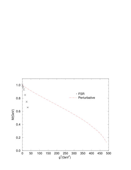
Fig. 18. : The coupling constant dependence of the 1-body dressed mass is shown. Beyond the critical coupling strength of $g^{2}=31$ ${\rm GeV}^{2}$ the 1-body mass becomes unstable. The perturbative bubble summation also has a critical point near $g^{2}=490$ ${\rm GeV}^{2}$.

In sampling trajectories the first step is termalization. In order to insure that the initial configuration of trajectories has no effect on results initial updates are not taken into account. Depending on the dimensionality of the problem and the coupling strength the number of initial updates neeeded for termalization is of the order of 1000 updates. [15] In order to satisfy self consistency regarding the location of the stationary point discussed earlier, the location of the stationary point must be determined carefully. The stationary point can be parametrized as $s_{0}=CT/(2m)$, where $T/2m$ is the location of the stationary point when the coupling strength $g$ goes to zero. As the coupling strength is increased the stationary point moves out (see Figs. 15, and  17 ) and eventually the critical point is reached beyond which there is no stationary point. In order to be able to do Monte-Carlo integrations an initial guess must be made for the location of the stationary point. Self consistency is realized by insuring that the peak location of the s distribution in the Monte-Carlo integration agrees with the initial guess for the stationary point. [15] In Fig. 17 the dependence of the location of the stationary point on the coupling strength is shown. Fig. 17 shows that beyond the critical point $g^{2}\simeq 31$ GeV² $C$ goes to infinity implying that there is no stationary point. A similar critical behavior was also observed in Refs. [20] within the context of a variational approach. In Fig. 18 exact 1-body dressed mass results are shown for $m_{\chi}=1$ GeV, $\mu_{\phi}=0.15$ GeV. Results indicate that the perturbative bubble summation deviates from the quenched FSR result very significantly. These results are all for a Pauli-Villars mass of 3$\mu$.

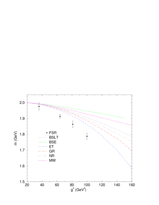
Fig. 19. : The coupling constant dependence of the 2-body bound state mass is shown. Beyond the critical coupling strength of $g^{2}=100$ GeV² the 2-body mass becomes unstable. The Bethe-Salpeter equation in the ladder approximation gives the lowest binding.

In Figure 19 we present the comparison of the 2-body bound state masses obtained by the FSR with various bound state equations. The FSR calculation involves summation of all ladder and crossed ladder diagrams, and excludes the self energy contributions. According to Figure 19 all bound state equations underbind. Among the manifestly covariant equations the Gross equation gives the closest result to the exact calculation obtained by the FSR method. This is due to the fact that in the limit of infinitely heavy-light systems the Gross equation effectively sums all ladder and crossed ladder diagrams. Equal-time equation also produces a strong binding but the inclusion of retardation effects pushes the Equal-time results away from the exact results (Mandelzweig-Wallace equation [19]). In particular the Bethe-Salpeter equation in the ladder approximation (BSE in Figure 19) gives the lowest binding. Similarly the Blankenbecler-Sugar-Logunov-Tavkhelidze equation [17, 18] (BSLT) gives a very low binding. A comparison of the ladder Bethe-Salpeter, Gross, and the FSR results shows that the exchange of crossed ladder diagrams plays a crucial role.

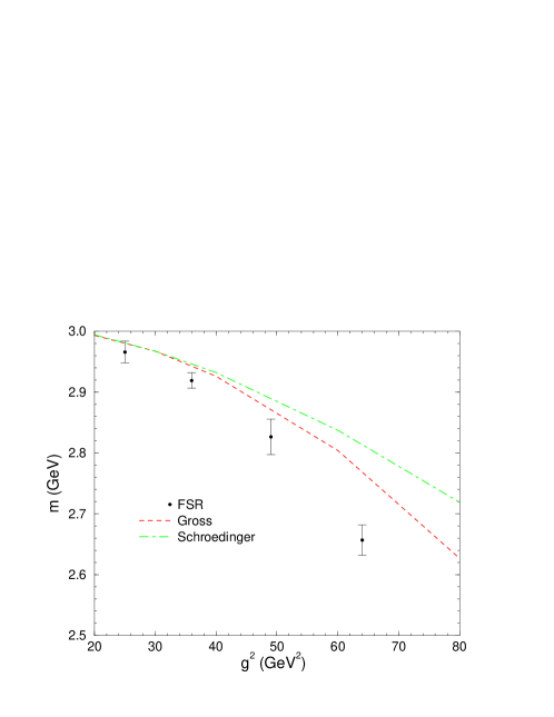
Fig. 20. : 3-body bound state results for 3 equal mass particles of mass 1 GeV.

In Figure 20 the 3-body bound state results for 3 equal mass particles of mass 1 GeV is shown. For 3-body case the only available results are the Schroedinger and Gross equation results. According to results presented in Figure 20 bound state equations underbind for the 3-body case too. Gross equation gives the closest result to the exact FSR result. Determination of the wavefunction of bound states is done by keeping the final state configurations of particles in a histogram. For example, for a 3-body bound state system, the probability distribution of the third particle for a given configuration of first and second particles is shown in Fig. 21. In the first plot of Fig. 21 two fixed particles are very close to each other such that the third particle sees them as a point particle. However as the fixed particles are separated from each other the third particle starts having a nonzero probability of being in between the two fixed particles (second and third plots of Fig. 21). Eventually when the two fixed particles are kept away from each other the third particle has a nonzero probability distribution only at the origin (the last plot shown in Fig. 21).

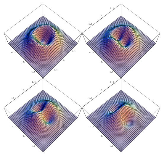
Fig. 21. : Evolution of the probability distribution for the 3rd particle is shown as the distance between the two fixed particles is increased. When the fixed particles are very close to each other the third particle sees them as a point particle (the upper left plot). As the fixed particles are separated from each other the third particle starts penetrating between them (2nd and 3rd plots), and as the two fixed particles are maximally separated the third particle spends most of its time in between the two fixed particles (the lower right plot).

Until this point the FSR method has been derived and various applications to nonperturbative problems have been presented. In the next section, as a check of the FSR method, we will obtain perturbative results using the FSR.

5 Perturbative expansion from the FSR approach

In this section we will show that perturbation theory results can be obtained from the FSR expressions. Let us first consider the perturbative expansion of the 1-body self energy in $\chi^{2}\phi$ interaction. The exact Greens function can be expanded in a power series in $g^{2}$:

$$G = \biggl{\lmoustache}_{0}^{\infty}\,ds\,\biggl{\lmoustache}{\cal D}z\,{\rm exp}\bigl{[}-m^{2}s-\frac{1}{4}\int_{0}^{s}d\tau z^{2}+\frac{g^{2}}{2}\int d\tau\int d\tau^{\prime}\Delta(z(\tau)-z(\tau^{\prime})\bigr{]}$$ (95)

$$= G^{(0)}+G^{(1)}+\cdots.$$

The leading contribution ($O(g^{0})$) is given by:

$$G^{(0)} = \biggl{\lmoustache}_{0}^{\infty}\,ds\,\biggl{\lmoustache}{\cal D}z\,{\rm exp}\bigl{[}-m^{2}s-\frac{1}{4}\int_{0}^{s}d\tau z^{2}\bigr{]},$$ (96)

$$= \biggl{\lmoustache}_{0}^{\infty}ds\biggl{(}\frac{N}{4\pi s}\biggr{)}^{2N}\Pi_{n=1}^{N-1}d^{4}z_{n}\,{\rm exp}\bigl{[}-m^{2}s-\frac{N}{4s}\sum_{i=1}^{N}(z_{i}-z_{i-1})^{2}\bigr{]}.$$

Noting that:

$$\biggl{\lmoustache}dz_{1}dz_{2}\cdots dz_{n}\,{\rm exp}\biggl{[}-\lambda\{(z_{1}-x)^{2}+(z_{2}-z_{1})^{2}+\cdots+(z_{n}-y)^{2}\}\biggr{]}$$

$$=\biggl{[}\frac{\pi^{n}}{(n+1)\lambda^{n}}\biggr{]}^{1/2},$$

all $z$ integrals can be performed and the free ($O(g^{0})$) propagator is found as

$$G^{(0)} = \biggl{\lmoustache}_{0}^{\infty}\frac{ds}{(4\pi s)^{2}}\,{\rm exp}\bigl{[}-m^{2}s-\frac{1}{4s}(x-y)^{2}\bigr{]}$$ (97)

$$= \frac{m}{4\pi^{2}|x-y|}K_{1}(m|x-y|),$$ (98)

which is the free propagator for a massive scalar particle in 3+1d. Now let us consider the next to leading order $O(g^{2})$ contribution to the 1-body propagator. Order $O(g^{2})$ term is given by

$$G^{(1)} = \frac{g^{2}}{2}\biggl{\lmoustache}_{0}^{\infty}ds\,\biggl{\lmoustache}{\cal D}z\,\biggl{\lmoustache}_{0}^{s}d\tau\biggl{\lmoustache}_{0}^{s}d\tau^{\prime}\,{\rm exp}\bigl{[}-m^{2}s-\frac{1}{4}\int_{0}^{s}d\tau z^{2}\bigr{]}\Delta(z(\tau)-z(\tau^{\prime})).$$

This expression has the following structure

$$G^{(1)} \equiv \frac{g^{2}}{2}\biggl{\lmoustache}_{0}^{\infty}ds\biggl{\lmoustache}_{0}^{s}d\tau\biggl{\lmoustache}_{0}^{s}d\tau^{\prime}f(s,\tau,\tau^{\prime}).$$ (99)

Using the identity

$$\biggl{\lmoustache}_{0}^{\infty}ds\biggl{\lmoustache}_{0}^{s}d\tau\,g(s,\tau)=\biggl{\lmoustache}_{0}^{\infty}ds\biggl{\lmoustache}_{0}^{\infty}d\tau\,g(s+\tau,\tau),$$ (100)

one may write

$$\biggl{\lmoustache}_{0}^{\infty}ds\biggl{\lmoustache}_{0}^{s}d\tau\biggl{\lmoustache}_{0}^{\tau}d\tau^{\prime}\,f(s,\tau,\tau^{\prime}) = \biggl{\lmoustache}_{0}^{\infty}ds\biggl{\lmoustache}_{0}^{\infty}d\tau\biggl{\lmoustache}_{0}^{\infty}d\tau^{\prime}\,f(s+\tau+\tau^{\prime},\tau+\tau^{\prime},\tau^{\prime}).$$

Therefore limits of all integrals in $G^{(1)}$ can be extended to infinity

$$G^{(1)} = g^{2}\biggl{\lmoustache}_{0}^{\infty}ds\biggl{\lmoustache}_{0}^{\infty}d\tau\biggl{\lmoustache}_{0}^{\infty}d\tau^{\prime}\,[f(s+\tau+\tau^{\prime},\tau+\tau^{\prime},\tau^{\prime})$$ (101)

Path integral in $G^{(1)}$ can be split into two regions using:

$$({\cal D}z)_{xy}=({\cal D}z)_{xz}\,d^{4}z\,({\cal D}z)_{zy}.$$ (102)

Therefore the full expression for $G^{(1)}$ takes the following form

$$G^{(1)} = g^{2}\biggl{\lmoustache}d^{4}z\biggl{\lmoustache}d^{4}z^{\prime}\,\Delta(z-z^{\prime})\biggl{\lmoustache}_{0}^{\infty}ds\biggl{\lmoustache}_{0}^{\infty}d\tau\biggl{\lmoustache}_{0}^{\infty}d\tau^{\prime}\biggl{\lmoustache}({\cal D}z)_{xz}({\cal D}z)_{zz^{\prime}}({\cal D}z)_{z^{\prime}y}$$

$$\times {\rm exp}\biggl{[}-m^{2}(s+\tau+\tau^{\prime})-\frac{1}{4}\int_{0}^{\tau^{\prime}}\dot{z}^{2}d\tau^{\prime\prime}-\frac{1}{4}\int_{\tau^{\prime}}^{\tau+\tau^{\prime}}\dot{z}^{2}d\tau^{\prime\prime}-\frac{1}{4}\int_{\tau+\tau^{\prime}}^{s+\tau+\tau^{\prime}}\dot{z}^{2}d\tau^{\prime\prime}\biggr{]},$$

where the intermediate boundary conditions are $z\equiv z(\tau^{\prime})$, and $z^{\prime}\equiv z(\tau+\tau^{\prime})$. All three path integrals in Eq. 5 can now be integrated to give three free propagators between points $(x-z-z^{\prime}-y)$

$$G^{(1)} = g^{2}\biggl{\lmoustache}d^{4}z\biggl{\lmoustache}d^{4}z^{\prime}\,\Delta(z-z^{\prime})S(x,z)S(z,z^{\prime})S(z^{\prime},y).$$ (104)

This is the correct perturbative 1-loop bubble expression, shown in Fig. 22, as expected.

Fig. 22. : The simplest bubble diagram

Next let us consider the tadpole diagram.

5.1 Leading order tadpole diagram from the FSR approach

The tadpole diagram exists only after unquenching. Consider the 1-body propagator,

$$G(y|x) = N\bigg{\lmoustache}{\cal D}\phi\,({\rm det}S)\,S(x,y)\,e^{-S[\phi]}.$$

In the quenched approximation det(S) is set equal to one. Here let us consider the next to leading order contribution to the quenched approximation. We can make the following expansion

$${\rm det}S = {\rm exp}\bigl{[}{\rm tr}({\rm log}S)\bigr{]}$$

$$\simeq 1+{\rm tr}({\rm log}S)+\frac{\left[{\rm tr}({\rm log}S)\right]^{2}}{2}+\cdots,$$

where the trace is defined by

$${\rm tr}({\rm log}S) = \biggl{\lmoustache}d^{4}x\left<x|{\rm log}S|x\right>.$$

Note that the trace is infinite and requires regularization, but this does not effect our discussion regarding the derivation of the perturbative result. Ordinary propagator has a path integral representation,

$$S = \bigg{\lmoustache}_{0}^{\infty}ds\,\bigg{\lmoustache}\,{\cal D}z\,\,{\rm exp}\biggl{[}-sm^{2}-\frac{1}{4}\int_{0}^{s}d\tau\,\dot{z}^{2}(\tau)-g\int_{0}^{s}d\tau\,\phi(z(\tau))\,\,\biggr{]}.$$

The logarithm of the propagator can also be expressed in the form of a path integral

$${\rm log}S=\bigg{\lmoustache}_{0}^{\infty}\frac{ds}{s}\,\bigg{\lmoustache}\,{\cal D}z\,\,{\rm exp}\biggl{[}-sm^{2}-\frac{1}{4}\int_{0}^{s}d\tau\,\dot{z}^{2}(\tau)-g\int_{0}^{s}d\tau\,\phi(z(\tau))\,\,\biggr{]}.$$

Therefore the diagram with 1-loop connected to the propagator can be written as

$$G(x,y) = \biggl{\lmoustache}_{0}^{\infty}ds\biggl{\lmoustache}_{0}^{\infty}\frac{ds_{l}}{s_{l}}\biggl{\lmoustache}({\cal D}z)_{xy}\biggl{\lmoustache}({\cal D}z_{l})\,{\rm exp}\biggl{[}-m^{2}s-m^{2}s_{l}$$

$$- \int_{0}^{s}\dot{z}^{2}\,d\tau-\int_{0}^{s_{l}}\dot{z}^{2}\,d\tau+g^{2}\int_{0}^{s}\oint_{0}^{s_{l}}\,d\tau\,d\tau_{l}\,\Delta(z(\tau)-z_{l}(\tau_{l}))\biggr{]}.$$

The next to leading order contribution to the 1-loop-1-particle connected propagator is given by

$$G(x,y) = g^{2}\biggl{\lmoustache}_{0}^{\infty}ds\biggl{\lmoustache}_{0}^{\infty}\frac{ds_{l}}{s_{l}}\biggl{\lmoustache}({\cal D}z)_{xy}\biggl{\lmoustache}({\cal D}z_{l})\,\biggl{\lmoustache}_{0}^{s}\,d\tau\biggl{\lmoustache}_{0}^{s_{l}}\,d\tau_{l}\,\Delta(z(\tau)-z_{l}(\tau_{l}))$$ (105)

$$\times\,{\rm exp}\biggl{[}-m^{2}s-m^{2}s_{l}-\int_{0}^{s}\dot{z}^{2}\,d\tau-\int_{0}^{s_{l}}\dot{z}^{2}\,d\tau\biggr{]},$$

where the loop trajectory $z_{l}$ is a circular trajectory and therefore has no fixed initial or final coordinates. Using the identity Eq. 100 and splitting the path integral as before one obtains

$$G(x,y)=g^{2}\biggl{\lmoustache}_{0}^{\infty}ds\biggl{\lmoustache}_{0}^{\infty}\frac{ds_{l}}{s_{l}+\tau_{l}}\biggl{\lmoustache}_{0}^{\infty}\,d\tau\biggl{\lmoustache}_{0}^{\infty}\,d\tau_{l}\,{\rm exp}\biggl{[}-m^{2}(s+s_{l}+\tau+\tau_{l})\biggr{]}$$

$$\times\biggl{\lmoustache}({\cal D}z)_{xz(\tau)}\,d^{4}z(\tau)\,({\cal D}z)_{z(\tau)y}\biggl{\lmoustache}\,d^{4}z_{0}\,({\cal D}z_{l})_{z_{0}z_{l}(\tau_{l})}\,d^{4}z_{l}(\tau_{l})\,({\cal D}z_{l})_{z_{l}(\tau_{l})z_{0}}$$

$$\times\Delta(z(\tau)-z_{l}(\tau_{l}))\,{\rm exp}\biggl{[}-\int_{0}^{\tau}\dot{z}^{2}\,d\tau-\int_{\tau}^{s+\tau}\dot{z}^{2}\,d\tau-\int_{0}^{\tau_{l}}\dot{z}_{l}^{2}\,d\tau-\int_{\tau_{l}}^{s_{l}+\tau_{l}}\dot{z}^{2}_{l}\,d\tau\biggr{]},$$

where the boundary conditions are

$$z(0)=x,\ \ z(\tau)=z,\ \ z(s+\tau)=y,$$ (106)

$$z_{l}(0)=z_{l}(s_{l}+\tau_{l})=z_{0},\ \ z_{l}(\tau_{l})=z_{l}.$$ (107)

Let us note that

$$\frac{{\rm exp}[-m^{2}(s+\tau)]}{s+\tau} = \biggl{\lmoustache}_{m^{2}}^{\infty}dm^{2}\,{\rm exp}[-m^{2}(s+\tau)].$$ (108)

With this replacement all path integrals can be evaluated easily, as done earlier in the 1-body self energy calculation, and the 1-loop Greens function to $O(g^{2})$ reduces to

$$G(x,y)=$$

$$g^{2}\biggl{\lmoustache}d^{4}z\biggl{\lmoustache}d^{4}z_{l}\,S(x,z)S(z,y)\Delta(z-z_{l})\biggl{\lmoustache}_{m^{2}}^{\infty}dm^{2}\,\biggl{\lmoustache}d^{4}z_{0}\,S_{m}(z_{0},z_{l})S_{m}(z_{l},z_{0}).$$

$z_{0}$ and $m^{2}$ integrals can be performed by noting that:

$$\biggl{\lmoustache}d^{4}z_{0}\,S_{m}(z_{0},z)S_{m}(z,z_{0}) = -\frac{\partial}{\partial m^{2}}S_{m}(z,z),$$ (109)

$$\lim_{m^{2}\rightarrow\infty}S_{m}(x,y) = 0.$$ (110)

Therefore the 1-loop diagram to $O(g^{2})$ is found as

$$G(x,y) = g^{2}\biggl{\lmoustache}d^{4}z\biggl{\lmoustache}d^{4}z_{l}\,S(x,z)S(z,y)\Delta(z-z_{l})S(z_{l},z_{l}),$$ (111)

which is the expected result from the perturbation theory, as shown in Fig. 23.

Fig. 23. : The leading order connected 1-loop diagram

This concludes the discussion of perturbative results within the FSR method. It should be clear that one may extend this discussion to higher order diagrams and obtain the correct perturbation theory results. It should be noted that unquenching to all orders in the FSR approach is numerically not feasable. This is related to the fact that the FSR approach relies on the discretization of trajectories. Every loop involved in the calculation represents a new discretized trajectory. Therefore inclusion of all loops is practically not possible. However one maybe be able to extract information about the effect of unquenching by making an expansion in the number of loops, that is by introducing loops order by order. More work needs to be done on this topic.

6 Conclusions

In these lectures the FSR representation has been introduced with various applications to scalar field theories. It has been shown that the FSR is an efficient and rigorous method for doing nonperturbative calculations in field theory. The FSR approach uses a covariant path integral representation for the trajectories of particles. Reduction of field theoretical path integrals to path integrals involving particle trajectories reduces the dimensionality of the problem and the associated computational cost. The FSR uses a space-time continuum. There are no boundaries in space-time and rotational symmetry is respected.

Applications of the FSR approach to 1 and 2-body problems in particular shows that uncontrolled approximations in field theory may lead to significant deviations from the correct result. Results presented here indicate that the ladder approximation for the 2-body bound state problem, and the rainbow approximation for the 1-body problem are both poor approximations. In both cases the crossed diagrams (such as crossed ladders) play an essential role.

Acknowledgements: I would like to thank the organizers of the 13th Indian-Summer School in Prague for inviting me to give a series of lectures, and for giving me a chance to experience the culture and the history of this beautiful city. This work was supported in part by the US Department of Energy under grant No. DE-FG02-97ER41032. Author thanks F. Gross and J. Tjon for useful discussions.

References

- [1] E.E. Salpeter, H.A. Bethe, Phys.Rev.84:1232-1242,1951
- [2] N. Nakanishi, Prog. Theor. Phys. Suppl. 43 (1969) 1; ibid 95, 1 (1988).
- [3] F. Gross, Phys. Rev. C 26 (1982), 2203.
- [4] F. Gross and J. Milana, Phys. Rev. D 43, 2401 (1991); 45, 969 (1992); 50, 3332 (1994).
- [5] P. C. Tiemeijer, J. A. Tjon, Phys. Rev. C 48 (1993); ibid C 49, 494 (1994).
- [6] H. J. Rothe, ’Lattice Gauge Theory’, World Scientific 1992.
- [7] R.P. Feynman, Phys. Rev 80 (1950), 440; J. Schwinger, Phys. Rev. 82 (1951), 664
- [8] Yu. A. Simonov, Nucl. Phys. B 307 512 (1988),
- [9] Yu. A. Simonov, Nucl. Phys. B 324 67 (1989).
- [10] Yu. A. Simonov and J. A. Tjon, Ann. Phys. 228, 1 (1993).
- [11] T. Nieuwenhuis, J. A. Tjon, Phys. Rev. Lett. 77, 814 (1996)
- [12] N. Brambilla, A. Vairo, Phys. Rev D. 56, 1445 (1997).
- [13] Ç Şavklı, J. A. Tjon, F. Gross, Phys. Review C 60 055210 (1999)
- [14] Ç Şavklı, F. Gross, J. A. Tjon, Phys. Review D 62 116006 (2000).
- [15] Ç Şavklı, hep-ph/9910502, ( accepted for publication in Comp. Phys. Comm.)
- [16] G. ’t Hooft, Nucl. Phys. B75 (1974)
- [17] A. A. Logunov, A. N. Tavkhelidze, Nuove Cimento 29, 380 (1963)
- [18] R. Blankenbecler, R. Sugar, Phys. Rev. 142, 1051 (1966).
- [19] S.J. Wallace, V.B. Mandelzweig, Nucl. Phys. A503, 673 (1989)
- [20] R. Rosenfelder, A.W. Schreiber, Phys. Rev. D 53 3337, 1996; Phys. Rev. D53, 3354, 1996.