Four–neutrino Oscillations at SNO

We discuss the potential of the Sudbury Neutrino Observatory (SNO) to constraint the four–neutrino mixing schemes favoured by the results of all neutrino oscillations experiments. These schemes allow simultaneous transitions of solar $\nu_{e}^{\prime}s$ into active $\nu_{\mu}$’s, $\nu_{\tau}$’s and sterile $\nu_{s}$ controlled by the additional parameter $\cos^{2}(\vartheta_{23})\cos^{2}(\vartheta_{24})$ and they contain as limiting cases the pure $\nu_{e}$–active and $\nu_{e}$–sterile neutrino oscillations. We first obtain the solutions allowed by the existing data in the framework of the BP00 standard solar model and quantify the corresponding predictions for the Charged Current and the Neutral Current to Charged Current event ratios at SNO in the different allowed regions as a function of the active–sterile admixture. Our results show that some information on the value of $\cos^{2}(\vartheta_{23})\cos^{2}(\vartheta_{24})$ can be obtained by the first SNO measurement of the CC ratio, while considerable improvement on the knowledge of this mixing will be achievable after the measurement of the NC/CC ratio.

I Introduction

The Sudbury Neutrino Observatory [1] is a second generation water Cerenkov detector using 1000 tonnes of heavy water, D₂O, as detection medium. SNO was designed to address the problem of the deficit of solar neutrinos observed previously in the Homestake [2], Sage [3], Gallex+GNO [4, 5] , Kamiokande [6] and Super–Kamiokande [7, 8] experiments, by having sensitivity to all flavours of neutrinos and not just to $\nu_{e}$, allowing for a model independent test of the oscillation explanation of the observed deficit.

Such sensitivity can be achievable because energetic neutrinos can interact in the D₂O of SNO via three different reactions. Electron neutrinos may interact via the Charged Current (CC) reaction

$$\nu_{e}+d\to p+p+e^{-}\ ,$$ (1)

with an energy threshold of several MeV. All non-sterile neutrinos may also interact via Neutral Current (NC)

$$\nu_{x}+d\to n+p+\nu^{\prime}_{x}\ ,\quad(x=e,\mu,\,\tau),$$ (2)

with an energy threshold of 2.225 MeV. With smaller cross section the non-sterile neutrinos can also interact via Elastic Scattering (ES) $\nu_{x}+e^{-}\to\nu^{\prime}_{x}+e^{-}$.

The main objective of SNO is to measure the ratio of NC/CC events. In its first year of operation SNO is concentrating on the measurement of the CC reaction rate while in a following phase, after the addition of MgCl₂ salt to enhance the NC signal, it will also perform a precise measurement of the NC rate. It is clear that a cross-section-normalized and acceptance-corrected ratio higher than 1 would strongly indicate the oscillation of $\nu_{e}$ into $\nu_{\mu}$ and/or $\nu_{\tau}$. On the other hand a deficit on both CC and NC leading to a normalized NC/CC ratio $1$, can only be made compatible with the oscillation hypothesis if $\nu_{e}$ oscillates in to a sterile neutrino.

There are several detailed studies in the literature of the potential of the SNO experiment to discriminate between the different oscillation solutions to the solar neutrino problem (SNP) [9, 10, 11, 12]. Most of these studies have been performed in the framework of oscillations between two neutrino states where $\nu_{e}$ oscillates into either an active, $\nu_{e}\to\nu_{a}$, or a sterile, $\nu_{e}\to\nu_{s}$, neutrino channel. On the other hand, once the possibility of a sterile neutrino is considered, these two scenarios are only limiting cases of the most general mixing structure [13, 14] which permits simultaneous $\nu_{e}\to\nu_{s}$ and $\nu_{e}\to\nu_{a}$ oscillations.

In this paper we study the potential of the Sudbury Neutrino Observatory to discriminate between active and sterile solar neutrino oscillations when analyzed in the framework of four–neutrino mixing. We consider those four–neutrino schemes favoured by considering together with the solar neutrino data, the results of the two additional evidences pointing out towards the existence of neutrino masses and mixing: the atmospheric neutrino data [15] and the LSND results [16]. We concentrate on two SNO measurements: the first expected result on the CC ratio and the expected to be most sensitive, the ratio of NC/CC. The measurement of other observables, such as the recoil energy spectrum of the CC events and the zenith angular dependence [9, 10, 11, 12] can provide important information to distinguish between the different allowed regions for $\nu_{e}$–active oscillations but they are not expected to be very sensitive as discriminatory between the active and sterile oscillations.

The outline of the paper is the following. For the sake of completeness we begin by discussing in Sec. II the expected results when obtained in the pure two–neutrino oscillation hypothesis. In Section III we determine the presently allowed regions for the oscillation solutions to the SNP in the framework of four–neutrino mixing. In Sec. IV we present the results of the expected CC and NC/CC rates for the different solutions and quantify the attainable sensitivity to the additional mixing controlling the admixture of active–sterile entering into the solar neutrino oscillations. Finally in Sec. V we summarize our conclusions.

II Two–Neutrino Mixing: Allowed Regions and Predictions for SNO

We first describe the results of the analysis of the solar neutrino data in terms of $\nu_{e}$ oscillations into either active or sterile neutrinos. We determine the allowed range of oscillation parameters using the total event rates of the Chlorine [2], Gallium [3, 4, 5] and Super–Kamiokande [7, 8] (corresponding to the 1117 days data sample) experiments. For the Gallium experiments we have used the weighted average of the results from GALLEX+GNO and SAGE detectors. We have also include the Super–Kamiokande electron recoil energy spectrum measured separately during the day and night periods. This will be referred in the following as the day–night spectra data which contains $18+18$ data bins. The analysis includes the latest standard solar model fluxes, BP00 model [17], with updated distributions for neutrino production points and solar matter density. For details on the statistical analysis applied to the different observables we refer to Ref. [18, 19]. Nevertheless, two comments on the statistical analysis are in order:
— In the present analysis we also include the contribution to the theoretical errors of the event rates arising from the small uncertainty in the measured $S_{0}$–factor for the reaction ¹⁶O(p,$\gamma$)¹⁷F which is new in the BP00 model as discussed in Ref. [17]. Following the standard procedure [20], we include this new source of uncertainty for the rates, that we denote as $C_{F}$, by adding a new fractional $1\sigma$ uncertainty $\Delta lnX_{C_{F}}=0.18$. Since this uncertainty affects in direct proportion to the ¹⁷F flux we correspondingly add a new line $\alpha_{iC_{F}}=\partial\Phi_{i}/\partial X_{C_{F}}$ to the response matrix, with values $\alpha_{\,{}^{17}F,C_{F}}=1$ and $\alpha_{iC_{F}}=0$ for all other fluxes.
– In the analysis of the day–night spectrum data we include the correlation between the systematic errors of the day and night bins which were conservatively ignored in Ref.[19]. Thus, we use the correlation matrix:

$$\sigma^{2}_{ij}=\delta_{ij}(\sigma^{2}_{i,stat}+\sigma^{2}_{i,uncorr})+\sigma_{i,exp}\sigma_{j,exp}+\sigma_{i,cal}\sigma_{j,cal}$$ (3)

where i and j run from 1 to 36 bins in the day–night spectra data. $\sigma_{i,stat}$ is the statistical error, and $\sigma_{i,uncorr}$ is the error due to uncorrelated systematic uncertainties. $\sigma_{i,exp}$ and $\sigma_{i,cal}$ are the correlated errors due to correlated systematic experimental uncertainties and the calculation of the expected spectrum respectively (see Ref. [18] for details). The addition of the correlations between the errors for the day and night bins, which more properly takes into account the day–night information, leads to stronger constraints on the regeneration region.

With all this we obtain that using the predicted fluxes from the BP00 model the $\chi^{2}$ for the total event rates is $\chi^{2}_{SSM}=56$ for 3 d. o. f. This means that the SSM together with the SM of particle interactions can explain the observed data with a probability lower than $5\times 10^{-12}$.

The allowed regions in the oscillation parameter space are shown in Fig. 1. We present them in the full parameter space for oscillations including both MSW[21] and vacuum[22] oscillations, as well as quasi-vacuum[23] oscillations (QVO) and matter effects for mixing angles in the second octant (the so called dark side [24, 14, 19]). In the case of $\nu_{e}$–active neutrino oscillations we find that the best–fit point is obtained for the LMA solution. There are two more local minima of $\chi^{2}$ in the MSW region: the SMA and LOW solutions. Notice also that LOW and QVO regions are connected at the 99 %CL and they extend into the second octant so maximal mixing is allowed at 99 % CL for $\Delta m^{2}$ in what we define as the LOW–QVO region.

Following the standard procedure, the allowed regions are defined in terms of shifts of the $\chi^{2}$ function with respect to the global minimum in the plane. Defined this way, the size of a region depends on the relative quality of its local minimum with respect to the global minimum but from the size of the region we cannot infer the actual absolute quality of the description in each region. In order to give this information we list in Table  I the goodness of the fit (GOF) for each solution obtained from the value of $\chi^{2}$ at the different minima.

For oscillations into sterile neutrinos the global minimum lies in the SMA solution. As seen in Fig. 1 we find that with the present data and using the criteria explained above, there are also allowed solutions for sterile neutrinos in the LMA and LOW–QVO regions at 99 %CL once the day–night spectra data is included. We consider, however, that they are not acceptable solutions as their fit to the global rates is really poor with a probability of acceptance less than 0.004 . The differences between both oscillation scenarios (active and sterile) can be easily understood. Unlike active neutrinos which lead to events in the Super–Kamiokande detector by interacting via NC with the electrons, sterile neutrinos do not contribute to the Super–Kamiokande event rates. Therefore a larger survival probability for ⁸B neutrinos is needed to accommodate the measured rate. As a consequence a larger contribution from ⁸B neutrinos to the Chlorine and Gallium experiments is expected, so that the small measured rate in Chlorine can only be accommodated if no ⁷Be neutrinos are present in the flux. This is only possible in the SMA solution region, since in the LMA and LOW regions the suppression of ⁷Be neutrinos is not enough. Notice also that the SMA region for oscillations into sterile neutrinos is slightly shifted downwards as compared with the active case. This is due to the small modification on the neutrino survival probability induced by the different matter potentials. The matter potential for sterile neutrinos is smaller than for active neutrinos due to the negative NC contribution proportional to the neutron abundance. For this reason the resonant condition for sterile neutrinos is achieved at lower $\Delta m^{2}$. On the other hand, the flatter spectrum, is better fitted in both LMA and LOW regions independently of the active or sterile nature of the neutrino. This leads to the improvement of the quality of the description for these solutions for both active and sterile neutrinos. However, as mentioned above, for the analysis of the total rates these LMA and LOW solutions give a very bad fit in the sterile case and we decide not to consider them in the following. Also, as we will see in next section, when the analysis is performed in the framework of four–neutrino oscillations those large mixing solutions for sterile neutrinos do not appear.

Next we quantify the predictions for the SNO observables in the allowed regions discussed above. The total number of events in the CC reaction at SNO can be obtained as

$$N^{th}_{CC} = \sum_{k=1,2}\phi_{k}\int\!dE_{\nu}\,\lambda_{k}(E_{\nu})\sigma_{CC}(E_{\nu})\langle P_{\nu_{e}\to\nu_{e}}\rangle$$ (4)

where $E_{\nu}$ is the neutrino energy, $\phi_{k}$ are the total neutrino ⁸B and hep fluxes, $\lambda_{k}$ is the neutrino energy spectrum (normalized to 1) and $\langle P_{\nu_{e}\to\nu_{e}}\rangle$ is the time–averaged $\nu_{e}$ survival probability for oscillations into either active or sterile neutrinos. Here $\sigma_{CC}$ is the $\nu$d CC cross section computed from the corresponding differential cross sections folded with the finite energy resolution function of the detector and integrated over the electron recoil energy:

$$\sigma_{CC}(E_{\nu})=\int_{T_{\text{th}}}\!dT\int\!dT^{\prime}\,Res(T,\,T^{\prime})\,\frac{d\sigma_{CC}(E_{\nu},\,T^{\prime})}{dT^{\prime}}\ ,$$ (5)

where T and T’ are the measured and the true kinetic energy of the recoil electrons and $T_{\text{th}}$ indicates the threshold expected from the experiment. The resolution function $Res(T,\,T^{\prime})$ is of the form [9]:

$$Res(T,\,T^{\prime})=\frac{1}{\sqrt{2\pi}(0.348\sqrt{T^{\prime}/\text{MeV}})}\exp\left[-\frac{(T-T^{\prime})^{2}}{0.242\,T^{\prime}\,{\text{MeV}}}\right]\ ,$$ (6)

and we take the differential cross section $d\sigma_{CC}(E_{\nu},\,T^{\prime})/dT^{\prime}$ from [26]. For definiteness,we adopted the most optimistic total energy threshold $E_{th}=5~{}MeV$ ($T_{th}=E_{th}-m_{e}$).

Correspondingly, the total number of events in the NC reaction at SNO is obtained as

$$N^{th}_{NC} = \sum_{k=1,2}\phi_{k}\int\!dE_{\nu}\,\lambda_{k}(E_{\nu})\sigma_{NC}(E_{\nu})(\langle P_{\nu_{e}\to\nu_{e}}\rangle+\langle P_{\nu_{e}\to\nu_{a}}\rangle)$$ (7)

where $\sigma_{NC}$ is the $\nu$d NC cross section from [26] and $\langle P_{\nu_{e}\to\nu_{a}}\rangle$ is the time–averaged probability of oscillation into any other active neutrino. In the case that $\nu_{e}$ oscillates only into active neutrinos $\langle P_{\nu_{e}\to\nu_{e}}\rangle+\langle P_{\nu_{e}\to\nu_{a}}\rangle$=1 and $N^{th}_{NC}$ is a constant.

In order to cancel out all energy independent efficiencies and normalizations we will use the ratio:

$$R^{th}_{CC} = \frac{N^{th}_{CC}}{N^{SSM}_{CC}}\equiv{\mbox{[CC]}}$$ (8)

where $N^{SSM}_{CC}$ is the predicted number of events in the case of no oscillations. The equivalent expression for the NC ratio

$$R^{th}_{NC} = \frac{N^{th}_{NC}}{N^{SSM}_{NC}}\equiv{\mbox{[NC]}}$$ (9)

Out of those ratios one can compute the double ratio $\frac{R^{th}_{NC}}{R^{th}_{CC}}\equiv$ [NC]/[CC] for which the largest sources of uncertainties cancel out  [11]. As it was shown in Ref. [26], the ratio between the NC and CC reaction cross sections is extremely stable against any variations of the inputs of the calculations. The expected total uncertainties for the [CC] ratio and the [NC]/[CC] ratio are 6.7 % and 3.6 % respectively assuming 5000 CC events and 1219 NC events [11].

In Fig. 2 we show the predicted [CC] and [NC]/[CC] ratios for the allowed regions in the two flavour analysis. The dots correspond to the local best fit points and the error bars show the range of predictions for the points inside the 90 and 99 %CL allowed regions. The mapping of the regions onto these bars can be easily understood from the behaviour of the probability for the different solutions:
(a) For oscillations into active neutrinos the [NC]/[CC] ratio is simply the inverse of the [CC] prediction. Therefore

• In the SMA region smaller mixing angles are mapped onto higher (lower) values of [CC] ([NC]/[CC]) ratio. One may notice that the prediction for the [CC] rate for the global best fit point (0.72) is larger than the measured rate at Super–Kamiokande. This is due to the nearly flat spectrum at Super–Kamiokande which implies that the best fit point in the global analysis corresponds to a smaller mixing angle than the best fit point for the analysis of rates only.

• In the LMA region, the lower $\Delta m^{2}$ and $\theta$ values are mapped onto higher (lower) [NC]/[CC] ([CC]) ratios and viceversa.

• In the LOW region the higher (lower) [NC]/[CC] ([CC]) ratio occurs for smaller $\theta$ and higher $\Delta m^{2}$.

(b) For the sterile case, the best fit point in SMA occurs at lower $\Delta m^{2}$ than in the active case and this produces a higher prediction for the [CC] ratio (0.74). The [NC]/[CC] ratio takes an almost constant value very close to one (0.98 in the best fit point), since both numerator and denominator are proportional to $\langle P_{\nu_{e}\to\nu_{e}}\rangle$. It is smaller than one because for the SMA solution the probability increases with energy in the range of detection at SNO and the threshold for the NC reaction is below the one for the CC one.

For the sake of consistency we have checked that our results agree perfectly with those in Ref. [11] when comparing the same points in the parameter space. However a careful reader may notice that the predictions at the best fit points and ranges in each region displayed in Fig. 2 are slightly different of those in Ref. [11]. The difference is due to two factors. First, the allowed regions are defined in a different way. In Ref. [11] departures from the standard solar model in the boron flux normalization are allowed and moreover the regions are defined in terms of shifts of the $\chi^{2}$ function with respect to the local minimum in the corresponding region. Second, the inclusion of the updated data, mainly the Super–Kamiokande day–night spectra, lowers the value of $\tan^{2}\theta$ for the best bit point in the SMA region by a factor  2 and increases $\Delta m^{2}$ for the best fit point in LMA by a factor  1.5.

What we see from these results is that while the data on [CC] can give a hint towards large or small mixing solutions, it will be hard to distinguish active from sterile oscillations on the only bases of this measurement. This is not the case for the [NC]/[CC] ratio where both scenarios appear nicely separated. It is not hard to foresee from these results that from the [NC]/[CC] measurement SNO will be able to constraint the additional mixings in the four–neutrino scenario which describe the admixture of active and sterile oscillations. This is the main point in this paper.

III Allowed Four–neutrino Mixing Parameters

Together with the results from the solar neutrino experiments we have two more evidences pointing out towards the existence of neutrino masses and mixing: the atmospheric neutrino data [15] and the LSND results [16]. All these experimental results can be accommodated in a single neutrino oscillation framework only if there are at least three different scales of neutrino mass-squared differences. The simplest case of three independent mass-squared differences requires the existence of a light sterile neutrino, i.e. one whose interaction with standard model particles is much weaker than the SM weak interaction, so it does not affect the invisible Z decay width, precisely measured at LEP.

There are six possible four–neutrino schemes that can accomodate all these evidences. They can be divided in two classes: 3+1 and 2+2. In the 3+1 schemes there is a group of three neutrino masses separated from an isolated mass by a gap of the order of 1eV which gives the mass-squared difference responsible for the short-baseline oscillations observed in the LSND experiment. In 2+2 schemes there are two pairs of close masses separated by the LSND gap. We have ordered the masses in such a way that in all these schemes $\Delta{m}^{2}_{\text{sun}}=\Delta{m}^{2}_{21}$ produces solar neutrino oscillations and $\Delta{m}^{2}_{\text{LSND}}=\Delta{m}^{2}_{41}$ (we use the common notation $\Delta{m}^{2}_{kj}\equiv m_{k}^{2}-m_{j}^{2}$). 3+1 schemes are disfavoured by experimental data with respect to the 2+2 schemes [27, 28] but they are still marginally allowed [29].

In any of these four-neutrino schemes the flavour neutrino fields $\nu_{\alpha L}$ (we choose $\alpha=e,s,\mu,\tau$) are related to the fields $\nu_{kL}$ of neutrinos with masses $m_{k}$ by a rotation $U$. $U$ is a $4{\times}4$ unitary mixing matrix, which contains, in general, 6 mixing angles and 3 CP violating phases (3 additional phases appear for Majorana neutrinos but they are irrelevant for oscillations). We neglect here the CP phases, which, in the schemes considered, are irrelevant for solar neutrinos because their effect is washed out by averaging over neutrino energy and distance. Existing bounds from negative searches for neutrino oscillations performed at colliders as well as reactor experiments, in particular the negative results of the Bugey [30] and CHOOZ [31] $\bar{\nu}_{e}$ disappearance experiment, impose severe constrains on the possible mixing structures for the four–neutrino scenario. In particular they imply that the matrix elements $U_{e3}$ and $U_{e4}$ are very small [27, 28, 32]. As a consequence, for any of these four–neutrino schemes, either 2+2 or 3+1, only four mixing angles are relevant in the study of solar neutrino oscillations [13, 14, 32] and the $U$ matrix can be written as

$$U=\left(\begin{array}[]{cccc}c_{12}&s_{12}&0&0\\ -s_{12}c_{23}c_{24}&c_{12}c_{23}c_{24}&s_{23}c_{24}&s_{24}\\ s_{12}(c_{23}s_{24}s_{34}+s_{23}c_{34})&-c_{12}(s_{23}c_{34}+c_{23}s_{24}s_{34})&c_{23}c_{34}-s_{23}s_{24}s_{34}&c_{24}s_{34}\\ s_{12}(c_{23}s_{24}c_{34}-s_{23}s_{34})&c_{12}(s_{23}s_{34}-c_{23}s_{24}c_{34})&-(c_{23}s_{34}+s_{23}s_{24}c_{34})&c_{24}c_{34}\end{array}\right)\,,$$ (10)

where $\vartheta_{12}$, $\vartheta_{23}$, $\vartheta_{24}$, $\vartheta_{34}$ are four mixing angles and $c_{ij}\equiv\cos\vartheta_{ij}$ and $s_{ij}\equiv\sin\vartheta_{ij}$.

Since solar neutrino oscillations are generated by the mass-square difference between $\nu_{2}$ and $\nu_{1}$, it is clear from Eq. (10) that the survival of solar $\nu_{e}$’s mainly depends on the mixing angle $\vartheta_{12}$, whereas the mixing angles $\vartheta_{23}$ and $\vartheta_{24}$ determine the relative amount of transitions into sterile $\nu_{s}$ or active $\nu_{a}$, this last one being a combination of $\nu_{\mu}$ and $\nu_{\tau}$ controlled by the mixing angle $\theta_{34}$. $\nu_{\mu}$ and $\nu_{\tau}$ cannot be distinguished in solar neutrino experiments, because their matter potential and their interaction in the detectors are equal, due only to NC weak interactions. As a consequence the active/sterile ratio and the survival probability for solar neutrino oscillations do not depend on the mixing angle $\vartheta_{34}$, and depend on the mixing angles $\vartheta_{23}$ $\vartheta_{24}$ only through the combination $\cos{\vartheta_{23}}\cos{\vartheta_{24}}$. For further details see Ref. [13, 14]. We distinguish the following limiting cases:
$\bullet$ $\cos{\vartheta_{23}}\cos{\vartheta_{24}}=0$ corresponding to the limit of pure two-generation $\nu_{e}\to\nu_{a}$ transitions.
$\bullet$ $\cos{\vartheta_{23}}\cos{\vartheta_{24}}=1$ for which we have the limit of pure two-generation $\nu_{e}\to\nu_{s}$ transitions.
$\bullet$ If $\cos{\vartheta_{23}}\cos{\vartheta_{24}}\neq 1$, solar $\nu_{e}$’s can transform in the linear combination $\nu_{a}$ of active $\nu_{\mu}$ and $\nu_{\tau}$.

In the general case of simultaneous $\nu_{e}\to\nu_{s}$ and $\nu_{e}\to\nu_{a}$ oscillations the corresponding probabilities are given by [13, 14]

$$P_{\nu_{e}\to\nu_{s}}=c^{2}_{23}c^{2}_{24}\left(1-P_{\nu_{e}\to\nu_{e}}\right)\,,$$ (11)

$$P_{\nu_{e}\to\nu_{a}}=\left(1-c^{2}_{23}c^{2}_{24}\right)\left(1-P_{\nu_{e}\to\nu_{e}}\right)\,.$$ (12)

where $P_{\nu_{e}\to\nu_{e}}$ takes the standard two–neutrino oscillation form for $\Delta m^{2}_{12}$ and $\theta_{12}$ but computed with the modified matter potential

$$A\equiv A_{CC}+c^{2}_{23}c^{2}_{24}A_{NC}\,.$$ (13)

Thus the analysis of the solar neutrino data in the four–neutrino mixing schemes is equivalent to the two–neutrino analysis but taking into account that the parameter space is now three–dimensional $(\Delta m^{2}_{12},\tan^{2}\vartheta_{12},\cos^{2}{\vartheta_{23}}\,\cos^{2}{\vartheta_{24}})$. We want to stress that, although originally this derivation was performed in the framework of the 2+2 schemes [13, 14], it is equally valid for the 3+1 ones [32].

We first present the results of the allowed regions in the three–parameter space for the global combination of observables. Notice that since the parameter space is 3–dimensional the allowed regions for a given CL are defined as the set of points satisfying the condition $\chi^{2}(\Delta m_{12}^{2},\vartheta_{12},c_{23}^{2}c_{24}^{2})-\chi^{2}_{min}\leq\Delta\chi^{2}\mbox{(CL, 3~{}dof)}$ where, for instance, $\Delta\chi^{2}($CL, 3 dof)=6.25, 7.83, and 11.36 for CL=90, 95, and 99 % respectively. In Figs. 3 we plot the sections of such volume in the plane ($\Delta{m}^{2}_{21},\tan^{2}(\vartheta_{12})$) for different values of $c_{23}^{2}c_{24}^{2}$. The global minimum used in the construction of the regions lies in the LMA region and for pure $\nu_{e}$–active oscillations, $c_{23}^{2}c_{24}^{2}=0$.

As seen in Fig. 3 the SMA region is always a valid solution for any value of $c_{23}^{2}c_{24}^{2}$ at 99% CL (the same is true at 95% CL). This is expected as in the two–neutrino oscillation picture this solution holds both for pure $\nu_{e}$–active and pure $\nu_{e}$–sterile oscillations. Notice, however, that the statistical analysis is different: in the two–neutrino picture the pure $\nu_{e}$–active and $\nu_{e}$–sterile cases are analyzed separately, whereas in the four–neutrino picture they are taken into account simultaneously in a consistent scheme. Since the GOF of the SMA solution for pure $\nu_{e}$–sterile oscillations is worse than for SMA pure active oscillations (as discussed in the previous section), the corresponding allowed region is smaller because they are now defined with respect to a common minimum. Also, we notice, that for the SMA solution the best scenario is a non-zero admixture between active and sterile oscillations. For this reason this solution is allowed at a CL better than 90 % only in the range $0.11\leq c_{23}^{2}c_{24}^{2}\leq 0.31$.

On the other hand, the LMA and LOW–QVO solutions disappear for increasing values of the mixing $c_{23}^{2}c_{24}^{2}$. We list in Table II the ranges of $c_{23}^{2}c_{24}^{2}$ for which each of the solutions is allowed at a given CL. We see that at 95 %CL the LMA solution is allowed for maximal active–sterile mixing $c_{23}^{2}c_{24}^{2}=0.5$ while at 99%CL all solutions are possible for maximal admixture.

IV Expected Rates at SNO in Four–Neutrino Schemes

In this section, we present the predictions for the CC ratio and for the NC/CC ratio in the four–neutrino scenario previously described. This scenario contains as limiting cases the pure $\nu_{e}$–active and $\nu_{e}$–sterile neutrino oscillations. However, when comparing the results for both limiting cases with the ones presented in Sec. II the reader must notice that there are some changes in the predicted ranges because the allowed regions are obtained with a different statistical criteria. Now, as discussed above, all the allowed regions are defined with respect to the same global minimum (laying in the LMA with $c_{23}^{2}c_{24}^{2}$=0) with 3 dof. Because of that, the predicted ranges in the four–neutrino scheme are wider for the pure $\nu_{e}$–active oscillations and narrower for the $\nu_{e}$–sterile case.

In Figs. 4$-$6 we show the results for the predicted [CC] ratio and [NC]/[CC] ratio for the different allowed regions (SMA, LMA, LOW-QVO) at 90 and 99 %CL as a function of $c_{23}^{2}c_{24}^{2}$. The general behaviour of the dependence of the predicted ratios with $c_{23}^{2}c_{24}^{2}$ can be easily understood using the following simplified expressions obtained from Eqs. (8), (9) and (11):

[CC] $$\sim P_{\nu_{e}\to\nu_{e}}\;,$$ (14)

$$\frac{\mbox{\rm[NC]}}{\mbox{\rm[CC]}} \sim \frac{1-c^{2}_{23}c^{2}_{24}(1-P_{\nu_{e}\to\nu_{e}})}{P_{\nu_{e}\to\nu_{e}}}\;.$$ (15)

From Eq. (14) we see that the only dependence of [CC] on $c_{23}^{2}c_{24}^{2}$ is due to the modification of the matter potential entering in the evolution equation (see Eq. (13) and discussion above) and it is very weak. The dependence of the allowed range of the [CC] ratio with $c_{23}^{2}c_{24}^{2}$ displayed in the figures arises mainly from the variation of the size of the allowed regions. Alternatively following Eq. (15) we find a stronger linear dependence of [NC]/[CC] on $c_{23}^{2}c_{24}^{2}$ with slope $(-1+P_{\nu_{e}\to\nu_{e}})/P_{\nu_{e}\to\nu_{e}}\sim 1-1/$[CC] and intercept $1/P_{\nu_{e}\to\nu_{e}}\sim 1/$[CC]. This simple description is able to reproduce the main features of our numerical calculations as can be seen in the figures.

Figs. 4$-$6 contain the main quantitative result of our analysis in the four–neutrino mixing scenario. From each of them it is possible to infer the allowed range of the active–sterile admixture, $c_{23}^{2}c_{24}^{2}$, compatible, within the expected uncertainty, with a given SNO measurement of the ratios. Also, comparing the allowed ranges for the different solutions one can study the potential of these measurements as discriminatory among the three presently allowed regions. Of course, both issues are not independent as we have no “a priory” knowledge of which is the right solution and both must be discussed simultaneously. In order to do so we pass to describe and compare in detail the predictions in the different regions.

The results for the SMA solution are shown in Fig. 4.a and 4.b for [CC] and [NC]/[CC] ratios respectively. First we notice that we find a small region allowed at 90 %CL only for a non–vanishing admixture of active and sterile oscillations as mentioned before. In this region [CC]$\sim$0.65–0.73 and [NC]/[CC]$\sim$ 1.3–1.4. The predictions at 99% range from [CC]$\sim$ 0.4–0.9 ([NC]/[CC]$\sim$1.1–2.5) for pure $\nu_{e}$–active scenario to to [CC]$\sim$ 0.59–0.85 ([NC]/[CC]$\sim$0.96–0.98) for pure $\nu_{e}$–sterile oscillations. Thus if SNO observes a ratio [CC]$<$0.58 the value of $c_{23}^{2}c_{24}^{2}$ can be constrained to be smaller than 1 disfavouring pure $\nu_{e}$–sterile oscillations. On the contrary a measurement of [CC]${}^{>}_{\sim}$0.68 will immediately hint towards the SMA solution but will not provide any information on the active–sterile admixture. Also, one must notice, that such value, although allowed by the present global statistical analysis at 99 %CL, will imply a strong disagreement with the total rate event rate observed at Super–Kamiokande.

As seen in Fig. 4.b the [NC]/[CC] ratio is more sensitive to the active–sterile admixture. To guide the eye, in the figures for the [NC]/[CC] ratio we plot a dotted line for the prediction in the case of no oscillation [NC]/[CC]=1. For any of the solutions, the allowed range for this ratio shows as general behaviour a decreasing with $c_{23}^{2}c_{24}^{2}$ due to two effects: $(i)$ the allowed regions become smaller and $(ii)$ the prediction decreases when more sterile neutrino is involved in the oscillations as described in Eq. (15). The measurement of higher values of this ratio will favour the four–neutrino scenario with larger component of $\nu_{e}$–active oscillations. On the other hand a measurement of [NC]/[CC]$\sim 1$, will push the oscillation hypothesis towards the pure $\nu_{e}$–sterile oscillation scenario. This case will be harder to differentiate from the non–oscillation scenario. We find that with the expected sensitivity the parameter $c_{23}^{2}c_{24}^{2}$ is constrained to be above 0.44 at 99% CL and that the pure $\nu_{e}$–active oscillations in the SMA region are compatible with [NC]/[CC]= 1 only at $\sim 5\sigma$.

The predictions for oscillation parameters in the LMA region are shown in Figs. 5.a and 5.b for [CC] and [NC]/[CC] ratios respectively. The predictions at 99% vary in the range [CC]$\sim$ 0.18–0.62 and [NC]/[CC]$\sim$ 1.4–5.6. The first thing we notice by comparing Fig. 5.a with Fig. 4.a and Fig. 6.a is that the most discriminatory scenario for the [CC] rate results if SNO finds a small value [CC]$\sim 0.25$. This would significantly hint towards the LMA solution to the solar neutrino problem and towards and $\nu_{e}$–active oscillation scenario. First, it is well separated from the predictions for the SMA and LOW regions. Second, it will include as a bonus a small but measurable day–night asymmetry [10, 11]. And third it will constrain the $c_{23}^{2}c_{24}^{2}$ to a small value ($\sim 0.2$). On the contrary the less discriminatory scenario will be a measurement 0.4$<$[CC]$<$0.6 where the prediction would be compatible with both SMA and LOW-QVO solutions and no improvement on our knowledge of the four–neutrino schemes is possible. The [NC]/[CC] ratio can definitively improve the discrimination between the different scenarios provided its measurement lies in the upper range. For instance a measurement of [NC]/[CC]$\sim$ 4 ($\pm$ 0.7 at $5\sigma$) will be conclusive for selecting LMA as the solution to the SNP and will imply and upper bound on $c_{23}^{2}c_{24}^{2}<0.3$.

The predictions for the LOW–QVO region lie between the ones for SMA and LMA as displayed in Fig. 6 and therefore they are more difficult to discriminate. The predictions at 99% vary in the range [CC]$\sim$ 0.3–0.68 and [NC]/[CC]$\sim$ 1.2–3.4. As a consequence we see that a low [CC] ratio but still within the 99% CL range allowed for this region, 0.3$<$[CC]$<$0.4, will constrain significantly the $c_{23}^{2}c_{24}^{2}$ parameter compatible with this solution but it will not be distinguishable from the LMA solution unless the measured [CC]$<$0.3. As mentioned above, the [NC]/[CC] ratio will be able to differentiate the LMA and LOW-QVO solutions if not in the range [1.5,3]. One should also notice that for the upper part of this range a positive measurement of the day–night asymmetry and the zenith dependence [12] will point towards the higher $\Delta{m}^{2}$ of the LOW region as the solution.

V Discussion

In this paper we have studied the potential of the Sudbury Neutrino Observatory to discriminate between active or sterile solar neutrino oscillations when analyzed in the framework of four–neutrino mixing. We considered those four–neutrino schemes favoured by considering together with the solar neutrino data, the results of the two additional evidences pointing out towards the existence of neutrino masses and mixing: the atmospheric neutrino data [15] and the LSND results [16]. These schemes allow simultaneous transitions of solar $\nu_{e}^{\prime}s$ into active $\nu_{\mu}$’s, $\nu_{\tau}$’s and sterile $\nu_{s}$ controlled by the additional parameter $\cos^{2}(\vartheta_{23})\cos^{2}(\vartheta_{24})$ and they contain as limiting cases the pure $\nu_{e}$–active and $\nu_{e}$–sterile neutrino oscillations. The allowed solar solutions have been reanalyzed including the recently BP00 standard solar model and the latest solar neutrino data. We find that the global minimum lies in the LMA region and for pure $\nu_{e}$–active oscillations ($c_{23}^{2}c_{24}^{2}=0$). We also find that in the framework of four–neutrino mixing the SMA solution is allowed at 90% CL for non vanishing active–sterile mixing $c_{23}^{2}c_{24}^{2}$ in the range [0.11,0.31].

We concentrated on two SNO measurements: the first expected result on the [CC] ratio and the expected to be most sensitive to the active–sterile admixture, the ratio of [NC]/[CC] and evaluated the predictions in the different regions as a function of the additional mixing $c_{23}^{2}c_{24}^{2}$. Our results are display in Figs. 4$-$6. They show that in most cases with the measurement of the [CC] ratio, it will be hard to improve the present knowledge of $c_{23}^{2}c_{24}^{2}$ but with the precise determination of the [NC/CC] ratio at SNO, this parameter can be strongly constrained for some of the allowed solutions. For example, we find that for the [CC] rate the most discriminatory scenario would be that SNO finds a small value [CC]$\sim 0.25$. This significantly hints towards the LMA solution to the solar neutrino problem and towards an active–active oscillation scenario. In this case the [NC]/[CC]$\sim$ 4 ($\pm$ 0.7 at $5\sigma$) will be conclusive for selecting LMA as the solution to the SNP and will imply and upper bound on $c_{23}^{2}c_{24}^{2}<0.3$. Conversely, a measurement of [NC]/[CC]$\sim 1$, although harder to distinguish from the non–oscillation scenario, will push the oscillation hypothesis towards the sterile SMA solution, and with the expected sensitivity a bound $c_{23}^{2}c_{24}^{2}>0.44$ at 99% CL can be imposed.

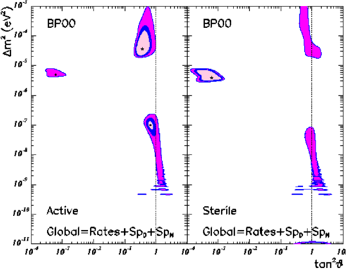
FIG. 1.: 90, 95 and 99 %CL allowed regions in the two–neutrino oscillation scenario from the global analysis of solar neutrino data including the total measured rates and the Super–Kamiokande measured spectrum at day and night. The global minimum is marked with a star while the local minima are denoted with a dot.

FIG. 2.: [CC] and [NC]/[CC] predictions at SNO for the allowed regions in the two–neutrino mixing scenarios obtained from the global analysis of solar neutrino data at 90 % and 99 %CL.

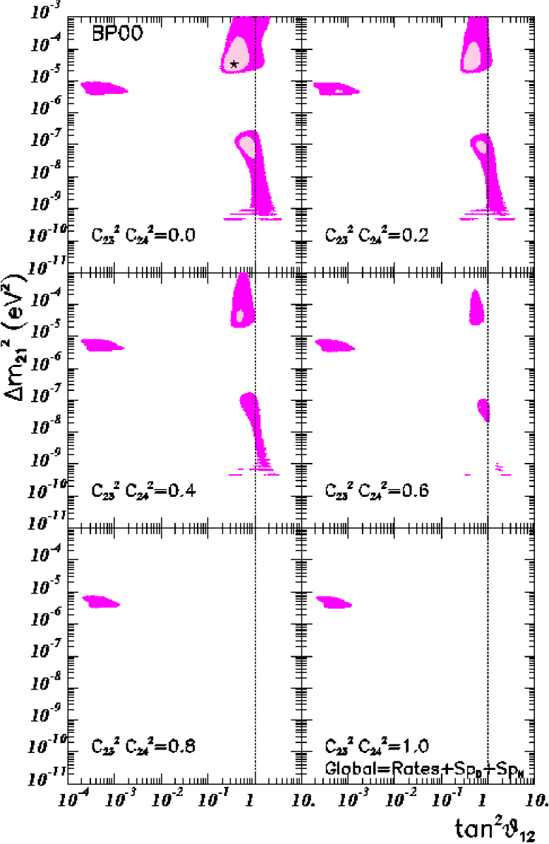
FIG. 3.: Results of the global analysis for the allowed regions in $\Delta{m}^{2}_{21}$ and $\sin^{2}\vartheta_{12}$ for the four–neutrino oscillations. The different panels represent the allowed regions at 90 % (lighter) and 99%CL (darker). The best–fit point in the three parameter space is plotted as a star.

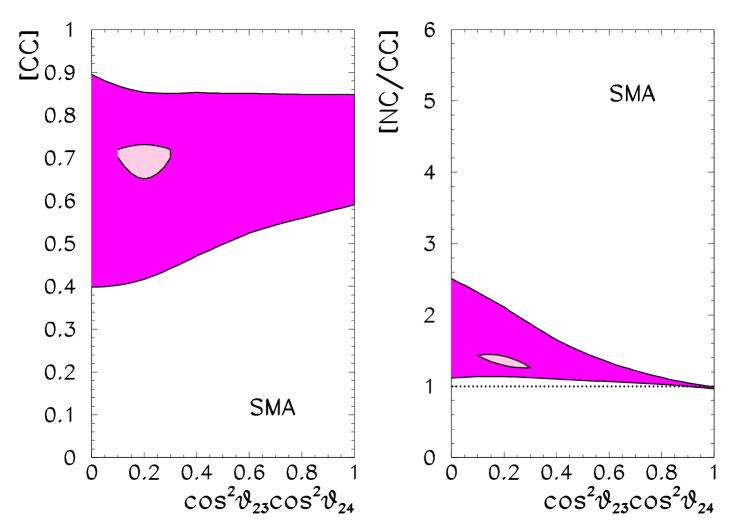
FIG. 4.: [CC] and [NC]/[CC] predictions at SNO as for the SMA region in the four–neutrino scenario obtained from the global analysis of solar neutrino data at 90 % (lighter) and 99 %CL (darker). The dotted line corresponds to the prediction in the case of no oscillations.

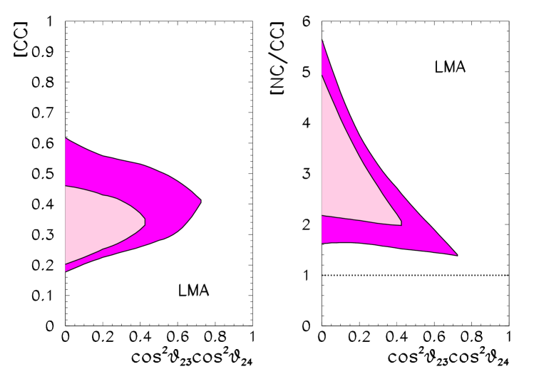
FIG. 5.: [CC] and [NC]/[CC] predictions at SNO as for the LMA region in the four–neutrino scenario obtained from the global analysis of solar neutrino data at 90 % (lighter) and 99 %CL (darker). The dotted line corresponds to the prediction in the case of no oscillations.

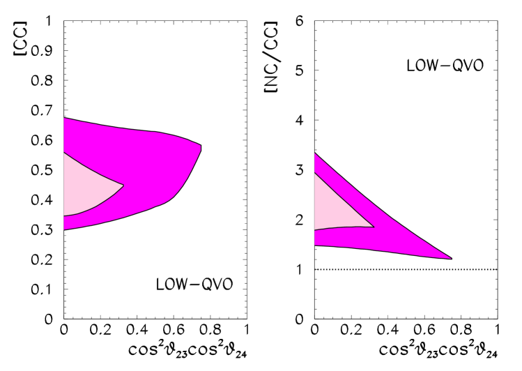
FIG. 6.: [CC] and [NC]/[CC] predictions at SNO as for the LOW region in the four–neutrino scenario obtained from the global analysis of solar neutrino data at 90 % (lighter) and 99 %CL (darker). The dotted line corresponds to the prediction in the case of no oscillations.

TABLE I.: Best fit points and GOF for the allowed solutions for the global analysis in the framework of two–neutrino mixing.

	Active			Sterile
	SMA	LMA	LOW-QVO	SMA
$\Delta m^{2}$/eV2	$5.0\times 10^{-6}$	$3.7\times 10^{-5}$	$1.0\times 10^{-7}$	$3.9\times 10^{-6}$
$\tan^{2}\theta$	0.00061	0.37	0.67	0.00061
$\chi_{min}$	40.8	33.4	37.1	42.3
Prob (%)	27 %	59 %	42 %	22 %

TABLE II.: Allowed ranges of $c^{2}_{23}c^{2}_{24}$ at 90%, 95%, and 99 % CL for the different solutions to the solar neutrino problem.

CL	SMA	LMA	LOW-QVO
90	[0.11,0.31]	[0,0.43]	[0,0.32]
95	[0,1]	[0,0.52]	[0,0.44]
99	[0,1]	[0,0.72]	[0,0.76]