Saclay-T00/166

BNL-NT-00/24

hep-ph/0011241

Nonlinear Gluon Evolution in the Color Glass Condensate: I Edmond Iancu,

Service de Physique Théorique, CEA Saclay, 91191 Gif-sur-Yvette, France

Andrei Leonidov

P. N. Lebedev Physical Institute, Moscow, Russia

Larry McLerran

Physics Department, Brookhaven National Laboratory, Upton, NY 11979, USA

We consider a nonlinear evolution equation recently proposed to describe the small-$x$ hadronic physics in the regime of very high gluon density. This is a functional Fokker-Planck equation in terms of a classical random color source, which represents the color charge density of the partons with large $x$. In the saturation regime of interest, the coefficients of this equation must be known to all orders in the source strength. In this first paper of a series of two, we carefully derive the evolution equation, via a matching between classical and quantum correlations, and set up the framework for the exact background source calculation of its coefficients. We address and clarify many of the subtleties and ambiguities which have plagued past attempts at an explicit construction of this equation. We also introduce the physical interpretation of the saturation regime at small $x$ as a Color Glass Condensate. In the second paper we shall evaluate the expressions derived here, and compare them to known results in various limits.

1 Introduction

There has been much activity in the last few years in an attempt to understand the physics of nuclear and hadronic processes in the regime where Bjorken’s $x$ becomes very small [1]–[25] (see also [26] for a pedagogical presentation and more references). The remarkable feature about this regime is that the gluon density in the hadron wavefunction becomes so high that perturbation theory breaks down even for a small coupling constant, by strong non-linear effects.

The important new phenomenon which is expected in these conditions is parton saturation [27, 28, 29], which is the fact that the density of partons per unit phase space $(dN/d^{2}p_{\perp}\,dy\,d^{2}x_{\perp})$ cannot grow forever as $x$ becomes arbitrarilly small [here, $y\equiv\ln(1/x)$ is the parton rapidity]. If this growth were to occur, then the cross section for deep inelastic scattering at fixed $Q^{2}$ would grow unacceptably large and eventually violate unitarity bounds. One rather expects the cross section to approach some asymptotic value at high energy, that is, to saturate. It is also intuitively obvious that this should happen, since if the phase space density becomes too large, repulsive interactions are generated among the gluons, and eventually it will be energetically unfavorable to increase the density anyfurther.

As $x$ becomes smaller and smaller, the gluon density increases faster, and is the driving force towards saturation. This is the reason why, in what follows, we shall concentrate exclusively on the gluon dynamics. Saturation is expected at a gluon phase-space density of order $1/\alpha_{s}\/$ [27, 7, 9], a value typical of condensates. This estimate, together with the fact that gluons are massless bosons, leads naturally to the expectation that the saturated gluons form a new form of matter, which is a Bose condensate. Since gluons carry color which is a gauge-dependent quantity, any gauge-invariant formulation will neccessarily involve an average over all colors, to restore the invariance. This averaging procedure bears a formal resemblance to the averaging over background fields done for spin glasses [30]. The new matter will be therefore called the Color Glass Condensate (CGC). This matter is universal in that it should describe the high gluon density part of any hadron wavefunction at sufficiently small $x$.

The CGC picture holds in a frame in which the hadron propagates at the speed of light and, by Lorentz contraction, appears as an infinitesimally thin two-dimensional sheet located at the light-cone. The formalism supporting this picture is in terms of a classical effective theory valid for some range of $x$, or longitudinal momentum $p^{+}$. In this theory, originally proposed by McLerran and Venugopalan to describe the gluon distribution in large nuclei [1], the valence quarks of the hadron (and, more generally, the “fast” partons, i.e., the partons which carry a large fraction of the hadron longitudinal momentum) are treated as sources for a classical color field which represents the small-$x$, or “soft”, gluons in the hadron wavefunction. The classical approximation is appropriate since the saturated gluons have large occupation numbers $\sim 1/\alpha_{s}$, and can thus be described by classical color fields with large amplitudes $A^{i}\sim 1/g$.

When going to smaller values of $x$, or lower longitudinal momenta $p^{+}$, one must integrate out the degrees of freedom associated with this change of scale [7]. This is done in perturbation theory for the quantum gluons (to leading logarithmic accuracy), but to all orders in the strong background fields $A^{i}$ which represent the condensate. This entails a change in the effective theory, which is governed by a functional, non-linear, evolution equation originally derived by Jalilian-Marian, Kovner, Leonidov and Weigert (JKLW) [10, 11]. This is a functional Fokker-Planck equation for the statistical weight function associated with the random variable $\rho_{a}(x)$ ($\equiv$ the effective color charge density of the fast gluons).

One of the consequences of the JKLW renormalization group equation it that it predicts the evolution of the gluon distribution function. In the low density, or weak-field limit, this equation linearizes and reduces to the BFKL equation [31], as shown in Ref. [10]. But in the saturation regime, where $A^{i}\sim 1/g$, the JKLW equation is fully non-linear, and will be discussed in great detail in this and the accompanying paper (to be referred to as “Paper I” and “Paper II” in what follows). In particular, in Paper II, we will show that this leads to the Balitsky-Kovchegov equation in the large-$N_{c}$ limit (with $N_{c}$ the number of colors). There is currently a discrepancy between the computations of Refs. [12, 13, 19, 22] and those by Balitsky [4] and Kovchegov [21]. The additional terms argued in [22] do actually not show up in our computation [32].

In the previous arguments, we have implicitly assumed the QCD coupling constant $\alpha_{s}$ to be small, which can be justified as follows: Associated with saturation, there is a characteristic transverse momentum scale $Q_{s}$ (a function of $x$), which is proportional to the density of gluons per unit area:

$$Q_{s}^{2}\,\propto\,{1\over{\pi R^{2}}}\,{{dN}\over{dy}}\,,$$ (1.1)

where $R$ is the radius of the hadron. $Q_{s}$ is the typical momentum scale of the saturated gluons, and increases with $1/x$ (see, e.g., Refs. [7, 9, 26]). Thus, for sufficiently small $x$, $Q_{s}^{2}\gg\Lambda^{2}_{QCD}$, and the coupling “constant” $\alpha_{s}(Q^{2}_{s})$ is weak indeed. (In any explicit calculation, the condition $Q_{s}^{2}\gg\Lambda^{2}_{QCD}$ must be verified a posteriori, for consistency.)

To summarize, the system under consideration is a weakly coupled high density system described by classical gluon fields. This is still non-perturbative, in the sense that the associated non-linear effects cannot be expanded in perturbation theory. But the non-perturbative aspects can now be studied in the simpler setting of a classical theory, via a combination of analytical and numerical methods (see, e.g., Refs. [1, 6, 7, 9, 20, 26]). In particular, in this context, it has been demonstrated [7, 9] that saturation occurs indeed, via non-linear dynamics.

The purpose of this paper and its sequel is twofold: first, to carefully rederive the JKLW evolution equation, by matching classical and quantum correlations; second, to render this equation precise and fully explicit, by computing its coefficients to all orders in the color field which describes the Color Glass Condensate. This requires an exact background field calculation which will be prepared by the analysis in Paper I, and presented in detail in Paper II.

Many of the results we shall present (especially in Paper I) are known in one form or another, and can be found in the literature. We shall nevertheless attempt to be comprehensive and pedagogical in our present treatment, in order to clarify several subtle points which have been often overlooked in the previous literature. To be specific, let us spell out here the new features of our analysis, to be presented below in this paper:

• The effective theory for the soft fields is stochastic Yang-Mills theory with a random color source localized near the light-cone ($x^{-}\simeq 0$) [see Sect. 2.1]. In previous work, this source has been generally taken as a delta function at $x^{-}=0$. Here, we find that in order to do a sensible computation, it is necessary at intermediate steps to spread out the source in $x^{-}$, that is, to take its longitudinal structure into account.

• For our ‘spread out’ source, we describe in detail the structure of the classical solution for the background field. We do this by relating the solution in the light cone gauge ($A^{+}=0$) to the solution in the covariant gauge ($\partial_{\mu}A^{\mu}=0$). We thus obtain an explicit expression for the background field in terms of the source in the covariant gauge [see Sect. 2.3]. This indicates that the source which is generated by quantum evolution must be evaluated in the covariant gauge as well.

• The quantum evolution of the effective theory is obtained by integrating out quantum fluctuations in a rapidity interval $\Delta y=\ln(1/b)$ (with $b\ll 1$) to leading order in $\alpha_{s}\ln(1/b)$, but to all orders in the strong background fields [cf. Sect. 3.2.1]. The quantum correlations induced in this way are then transferred to the stochastic classical theory, via a renormalization group equation of the Fokker-Planck type [cf. Sect. 3.2.2]. To prove the equivalence between the classical and quantum theories, we explicitly compute the induced field correlators $\langle A^{i}A^{j}\dots\rangle$ in both theories and show that they are the same, to the order of interest [cf. Sect. 3.2].

• The original JKLW renormalization group equation is written in terms of the color source in the light-cone gauge [11]. When reexpressing this equation in terms of the source in the covariant gauge, we find that we must subtract out a term related to classical vacuum polarization, so that the classical and quantum theory properly match [see Sect. 3.3].

• The non-linear evolution equation involves functional differentiations with respect to the source strength. With sources spread out and with explicit results from the covariant gauge, we have an explicit and transparent definition of these functional differentiations [see Sect. 3.2.2].

• The background fields are independent of the light-cone time $x^{+}$, but inhomogeneous, and even singular, in $x^{-}$. To cope with that, we find that it is more convenient to integrate the quantum fluctuations in layers of $p^{-}$ (the light-cone energy), rather than of $p^{+}$ [cf. Sect. 3.4]. Accordingly, we have no ambiguity associated with possible singularities at $p^{-}=0$.

• The gauge-invariant action describing the coupling of the quantum gluons to the classical color source is non-local in time [10]. Thus, the proper formulation of the quantum theory is along a Schwinger-Keldysh contour in the complex time plane [cf. Sect. 4]. However, in the approximations of interest, and given the specific nature of the background, the contour structure turns out not to be essential, so one can restrict oneself to the previous formulations in real time [10, 11].

• We carefully fix the gauge in the quantum calculations. In the light-cone gauge, the gluon propagator has singularities at $p^{+}=0$ associated with the residual gauge freedom under $x^{-}$–independent gauge transformations. We resolve these ambiguities by using a retarded $i\epsilon$ prescription [cf. eq. (3.4) and Sect. 6.3], which is chosen for consistency with the boundary conditions imposed on the classical background field. We could have equally well used an advanced prescription. However, other gauge conditions, such as Leibbrandt-Mandelstam or principal value prescriptions, are for a variety of technical reasons shown to be unacceptable [32].

• The choice of a gauge prescription has the interesting consequence to affect the spatial distribution of the source in $x^{-}$, and thus to influence the way we visualize the generation of the source via quantum evolution. With our retarded prescription, the source has support only at positive $x^{-}$ [see Sect. 5.1].

• We verify explicitly that the obtention of the BFKL equation as the weak-field limit of the general renormalization group equation is independent of the gauge-fixing prescription [cf. Sect. 5].

Once these various points are properly understood, the background field calculation in Paper II becomes unambiguous and well defined. As a result of this calculation, the coefficients in the JKLW equation will be obtained explicitly in terms of the color source in the covariant gauge [32]. With such explicit expressions in hand, we hope that the functional evolution equation can be solved, via analytic or numerical methods, or both, at least in particular limits. In fact, as we shall see in Paper II, in the large $N_{c}$ limit our results become equivalent to the equation proposed by Balitsky [4] and Kovchegov [21], for which an analytic solution has been recently given [23].

The ultimate goal of this and related analyses is to derive the properties of hadronic physics at arbitrarily high energies from first principles, that is, from QCD. We conjecture that there will be universal behaviour for all hadrons in the high energy limit. The work we present here is a step in proving this, and in developing a formalism which allows for explicit calculations in the saturation regime.

The present paper is organized as follows: In Section 2, we discuss the solution to the classical Yang-Mills equations with a color source which define the Mclerran-Venugopalan model. In Section 3, we derive the non-linear evolution equation by matching classical and quantum correlations. In Section 4, we formulate the quantized version of the Mclerran-Venugopalan model (on a complex-time contour), and derive Feynman rules for the coefficients of the renormalization group equation. In Section 5, we use the weak field, or BFKL, limit of the general evolution equations to test properties like the longitudinal distribution of the induced source, the equivalence between the renormalization group analysis in $p^{+}$ and in $p^{-}$, and the sensitivity to the $i\epsilon$ prescription in the LC-gauge propagator. In Section 6, we explicitly construct the gluon propagator in the presence of the background field describing the Color Glass Condensate. This propagator is the main ingredient of the quantum calculations to be presented in Paper II [32].

2 The classical approximation

In this section, we shall introduce the McLerran-Venugopalan model [1] for the gluon distribution at small $x$. This is classical Yang-Mills theory with a random color source, which is the effective color charge of the partons having longitudinal momenta larger than the scale of interest. This simple model, which is motivated by the separation of scales in the infinite momentum frame (see Sect. 2.1), offers an explicit scenario for saturation [7, 9] (see Sect. 2.4) which supports the physical picture of the Color Glass Condensate. The MV model will be further substantiated by the analysis in Sect. 3, where we shall see that this model is consistent with the quantum evolution towards small $x$ [7, 10, 11].

2.1 The McLerran-Venugopalan model

We consider a hadron in the infinite momentum frame (IMF), and in the light-cone (LC) gauge $A^{+}_{a}=0$, where the parton model is conventionally formulated (this gauge choice will be further motivated in Sect. 2.4). The hadron four-momentum reads $P^{\mu}=(P,0,0,P)$ (we neglect the hadron mass), or, in LC vector notations, which we shall use systematically from now on, $P^{\mu}\equiv(P^{+},P^{-},{\bf P}_{\perp})=({\sqrt{2}}P,0,{\bf 0}_{\perp})$. The fast partons, that is, the hadron constituents which, like the valence quarks, carry a relatively large fraction of the hadron longitudinal momentum $P^{+}$, move as almost free particles with momenta collinear with $P^{\mu}$, and act as sources for soft gluons, i.e., gluons with small longitudinal momenta $q^{+}\ll P^{+}$, which are probed in deep inelastic scattering (DIS).

For what follows, it is useful to have a sharp distinction between “fast” and “soft” modes in the hadron wavefunction, according to their $p^{+}$-momentum: to this aim we introduce an intermediate scale $\Lambda^{+}$ and define fast (soft) modes to have $p^{+}>\Lambda^{+}$ (respectively, $p^{+}<\Lambda^{+}$). We choose $\Lambda^{+}=x_{0}P^{+}$, with $x_{0}$ not too small; in fact, the main constraint on $x_{0}$ is to be much larger than the Bjorken parameter $x$ of the external probe that the hadron is interacting with.

For instance, in DIS, this probe is the virtual photon $\gamma^{*}$, with virtuality $Q^{2}\equiv-q^{\mu}q_{\mu}$. The Bjorken $x$ variable is defined as $x\equiv Q^{2}/2P\cdot q$ and, by kinematics, it coincides with the longitudinal momentum fraction $p^{+}/P^{+}$ of the struck parton. In what follows, we shall always assume that $x\ll 1$. Rather than a virtual photon, which couples to the charged constituents of the hadron (quarks and antiquarks), it is more convenient to consider a DIS initiated by the “current” $j\equiv-{1\over 4}F^{\mu\nu}_{a}F^{a}_{\mu\nu}$ which couples directly to gluons [9]. Indeed, we are mainly interested here in the gluon distribution, which is the dominant component of the hadron wavefunction when $x\ll 1$.

In the MV model, one assumes that the soft gluons can be described as the classical color fields $A^{\mu}_{a}$ radiated by the fast partons, themselves represented by a random color source $\rho_{a}$. As we shall demonstrate in Sect. 3, this assumption is indeed justified (at least to lowest order in $\alpha_{s}$) provided the MV model is used as an effective theory valid for some range of soft momenta. Then, the fast degrees of freedom are treated as quantum, but they are integrated out (perturbatively) in the construction of the effective theory, while the soft modes are non-perturbative, because of their large occupation numbers, but can be treated as classical, for this same reason. Via this construction, to be detailed in Sects. 3 and 4, the classical source $\rho_{a}$ will emerge as a natural way to describe the effects of the fast modes on the dynamics of the soft ones. In the original MV model [1], this source has been simply postulated, and its properties have been inferred via an analysis of the separation of scales in the problem. Since this separation will play a major role in what follows, let us briefly discuss it here:

The fast partons move along the $z$ axis with large $p^{+}$ momenta. They can emit, or absorb, soft gluons, but in a first approximation they do not deviate from their light-cone trajectories at $z=t$, or $x^{-}=0$ (no recoil, or eikonal approximation). Thus, they generate a color current only in the $+$ direction: $J_{a}^{\mu}=\delta^{\mu+}J^{+}_{a}$.

As quantum fields, the fast partons are delocalized in the $x^{-}$ direction within a distance $\lambda^{-}\sim 1/p^{+}$. However, when “seen” by the external probe or by the soft gluons (with momenta $q^{+}\ll p^{+}$, and therefore a poor longitudinal resolution), they appear as sharply localized at the light cone, within a distance $\Delta x^{-}\sim 1/\Lambda^{+}$. (This can be also understood as an effect of the Lorentz contraction). In some cases, to be carefully justified later, the associated current $J^{+}$ can be represented as a $\delta$ function at the light cone: $J^{+}\propto\delta(x^{-})$. But in general, it turns out that the longitudinal extent of the source cannot be neglected: this will be important both for the classical calculations in this section, and for the quantum analysis to be performed in the subsequent sections, and in Paper II.

Consider also the relevant LC-time scales: for on-shell excitations, $2p^{+}p^{-}=p_{\perp}^{2}$, which implies that softer gluons have larger energies $p^{-}\sim Q^{2}_{\perp}/p^{+}$, and therefore shorther lifetimes $\Delta x^{+}\sim 1/p^{-}\sim p^{+}\sim x$. Over such a short time interval, the “fast” partons are only slowly varying (since they have smaller energies), so their dynamics is essentially frozen. Thus, the soft gluons, or the external current in DIS, can probe only the equal-time correlators of the fast partons. All such correlators can be generated by a static current $J^{+}$ (quenched approximation).

To summarize, the soft color current due to the fast partons is expected with the following structure:

$$J_{a}^{\mu}(x)=\delta^{\mu+}\rho_{a}(x^{-},{\bf x}_{\perp}),\,\,\,\,\,\partial^{-}\rho_{a}\equiv{\partial\rho_{a}\over\partial x^{+}}=0,\,\,\,\,\,{\rm supp}\,\rho_{a}=\{x^{-}|0\leq x^{-}\leq 1/\Lambda^{+}\},\,\,$$ (2.1)

which will be confirmed by the quantum analysis in Sect. 3–5 and Paper II. Note the restriction of the support of $\rho$ to positive values of $x^{-}$. We shall see later that the precise longitudinal structure of the color source depends upon the gauge-fixing prescription, i.e., the condition used to completely fix the residual gauge freedom in the LC gauge. [Recall that, even after imposing the LC gauge, one still has the possibility to perform $x^{-}$–independent (or “residual”) gauge transformations, which preserve the condition $A^{+}=0$. In quantum calculations, fixing this residual gauge freedom amounts to chosing a prescription for the pole of the gluon propagator at $p^{+}=0$.] With the specific prescription that we shall adopt (cf. Sects. 3.4 and 6.3), the source $\rho$ is located at positive $x^{-}$, as anticipated in eq. (2.1).

The current (2.1) acts as a source for the Yang-Mills equations describing the soft gluon dynamics:

$$[D_{\nu},F^{\nu\mu}]\,=\,\delta^{\mu+}\rho_{a}(x^{-},{\bf x}_{\perp})\,.$$ (2.2)

To have a gauge-invariant formulation, the source $\rho_{a}$ must be treated as a stochastic variable with zero expectation value. This is also consistent with the physical interpretation of $\rho_{a}$ as the instantaneous color charge of the fast partons “seen” by the shortlived soft gluons, at some arbitrary time. The (spatial) correlators of the classical variable $\rho_{a}(\vec{x})$, with ${\vec{x}}\equiv(x^{-},{\bf x}_{\perp})$, are inherited from the (generally time-dependent) quantum correlations of the fast gluons. The precise scheme for transforming quantum into classical correlations will be explained in Sect. 3. Here, we shall simply summarize the ensuing classical correlations in some (not yet specified) weight function for $\rho_{a}$, denoted as $W_{\Lambda}[\rho]$. This is gauge-invariant by assumption, and depends upon the separation scale $\Lambda^{+}$ since it is obtained by integrating out quantum fluctuations with longitudinal momenta $|p^{+}|>\Lambda^{+}$ (cf. Sect. 3).

To conclude, in the MV model, the small-$x$ gluon correlation functions are obtained in two steps: (i) First, one solves the classical Yang-Mills equations (2.2) in the light-cone gauge $A^{+}=0$. The solution will be some non-linear functional of $\rho$, which we denote as ${\cal A}^{i}(\vec{x})[\rho]$. (Indeed, as we shall see in Sect. 2.3, one can always construct a solution which has $A^{-}=0$ and is time-independent.) (ii) The correlation functions of interest are evaluated on this classical solution, and then averaged over $\rho$, with the weight function $W_{\Lambda}[\rho]$ :

$$\langle A^{i}_{a}(x^{+},\vec{x})A^{j}_{b}(x^{+},\vec{y})\cdots\rangle_{\Lambda}\,=\,\int{\cal D}\rho\,\,W_{\Lambda}[\rho]\,{\cal A}_{a}^{i}({\vec{x}}){\cal A}_{b}^{j}({\vec{y}})\cdots\,.$$ (2.3)

The normalization here is such as

$$\int{\cal D}\rho\,\,W_{\Lambda}[\rho]\,=\,1.$$ (2.4)

Note that only equal-time correlators of the transverse fields can be computed in this way; but these are precisely the correlators which matter for the calculation of the gluon distribution function, cf. Sect. 2.4.

Note furthermore that the correlations obtained in this way depend upon the scale $\Lambda^{+}$. As we shall argue in Sect. 3 below, the effective theory in eqs. (2.2)–(2.3) is valid only at soft momenta of order $\Lambda^{+}$ (that is, at momenta $p^{+}\mathrel{\hbox to0.0pt{\raise 2.20013pt\hbox{$<$}\hss}{\lower 2.20013pt\hbox{$\sim$}}}\Lambda^{+}$, but not too far below $\Lambda^{+}$). Indeed, if one goes to the much softer scale $b\Lambda^{+}$ with $b\ll 1$, then there are large radiative corrections, of order $\alpha_{s}\ln(1/b)$, which invalidate the classical approximation at the scale $\Lambda^{+}$. In order to compute correlations at the new scale $b\Lambda^{+}$, one must first construct the effective theory valid at this scale, by integrating out the quantum degrees of freedom with longitudinal momenta in the strip $b\Lambda^{+}<|p^{+}|<\Lambda^{+}$. Once this is done, the dependence upon the intermediate scale $\Lambda^{+}$ goes away, as it should. This will be explained in detail in Sects. 3 and 4.

Remarkably, the equations (2.2)–(2.3) above are those for a glass (here, a color glass): There is a source, and the source is averaged over. This is entirely analogous to what is done for spin glasses when one averages over background magnetic fields [30]. To argue that one also has a condensate, one has to compute the correlation function (2.3). By using a Gaussian approximation for the weight function, one has found a saturation regime where the classical field has a typical strength of order $1/g$ [7, 9, 26] (see also Sect. 2.4 below). This is the maximal occupation number for a classical field, since larger occupation numbers are blocked by repulsive interactions of the gluon field. For weak coupling, this occupation number is large, and the gluons can be thought of as in some condensate. We are therefore lead to conclude that the matter which describes the small $x$ part of a hadron wavefunction is a Color Glass Condensate.

2.2 The Abelian case, as a warm up

Before attempting to solve the Yang-Mills equation (2.2), it is instructive to consider its Abelian version in some detail. This reads:

$$\partial_{\nu}F^{\nu\mu}=\delta^{\mu+}\rho({\vec{x}})$$ (2.5)

with $F^{\mu\nu}=\partial^{\mu}A^{\nu}-\partial^{\nu}A^{\mu}$ and ${\vec{x}}\equiv(x^{-},{\bf x}_{\perp})$.

We are interested in LC-gauge ($A^{+}=0$) solutions which vanish as $\rho\to 0$. Since $\rho$ is static (i.e., independent of $x^{+}$), we can look for solutions which are static as well: $\partial^{-}A^{\mu}=0$. Then, the components of eq. (2.5) with $\mu=-$ and $\mu=i$ imply that $A^{-}=0$ (so that $F^{-+}=F^{i-}=0$), and also $F^{ij}=0$. Thus, only the transverse fields $A^{i}({\vec{x}})$ are non-vanishing, and define a “pure gauge” in the two-dimensional transverse plane. We can thus write [throughout this paper, we shall systematically use calligraphic letters (like ${\cal A}^{i}$ and ${\cal F}^{i+}$) to denote solutions of the classical equations of motion] :

$${\cal A}^{i}({\vec{x}})=-\partial^{i}\omega({\vec{x}})$$ (2.6)

with $\omega({\vec{x}})$ satisfying the following equation (cf. eq. (2.5) with $\mu=+$ and $F^{i+}=-\partial^{+}A^{i}$):

$$-\nabla_{\perp}^{2}(\partial^{+}\omega)=\rho$$ (2.7)

Eq. (2.7) can be easily solved in momentum space, to give:

$${\cal A}^{i}(p)=ip^{i}\omega(p)=-{p^{i}\over p^{+}}{\rho(p^{+},p_{\perp})\over p_{\perp}^{2}}\,,$$ (2.8)

where, however, one needs a prescription to handle the pole at $p^{+}=0$. For instance, with the following, retarded prescription (with $\varepsilon\to 0_{+}$):

$${1\over p^{+}}\,\equiv\,{1\over p^{+}\ +i\varepsilon}\,,$$ (2.9)

one obtains a solution which vanishes at $x^{-}\to-\infty$ (thus, the “retardation” property refers here to $x^{-}$, and not to time) :

$${\cal A}^{i}(x^{-},x_{\perp})=\int_{-\infty}^{x^{-}}dy^{-}\,\partial^{i}\alpha(y^{-},x_{\perp})\,,$$ (2.10)

with $\alpha({\vec{x}})$ satisfying

$$-\nabla_{\perp}^{2}\alpha({\vec{x}})=\rho({\vec{x}}).$$ (2.11)

This yields $\alpha({\vec{p}})=\rho({\vec{p}})/p_{\perp}^{2}$ (with $\vec{p}\equiv(p^{+},{\bf p}_{\perp})$), or, in coordinate space,

$$\alpha({\vec{x}})\,=\,-\int{d^{2}y_{\perp}\over 2\pi}\,\ln\Bigl{(}|{\bf x}_{\perp}-{\bf y}_{\perp}|\mu\Bigr{)}\,\rho(x^{-},{\bf y}_{\perp}),$$ (2.12)

where $\mu$ is an infrared cutoff which must disappear from physical quantities.

In general, different prescriptions for the pole in $1/p^{+}$ correspond to different boundary conditions in $x^{-}$, which nevertheless describe the same physical situation, since they lead to the same electric field ${\cal F}^{i+}=-\partial^{+}{\cal A}^{i}=\partial^{i}\alpha\,$. Alternatively, solutions corresponding to different such prescriptions are related by (residual) gauge transformations.

Note finally that if the external source is localized around $x^{-}=0$ (cf. eq. (2.1)), so is $\alpha({\vec{x}})$, and therefore the associated electric field ${\cal F}^{i+}({\vec{x}})=\partial^{i}\alpha({\vec{x}})$.

2.3 The non-Abelian case

We now return to the non-Abelian problem, and note first that, written as it stands, eq. (2.2) is not really consistent: The property $[D_{\mu},[D_{\nu},F^{\nu\mu}]]=0$ requires the color current $J^{\mu}$ in the Yang-Mills equations to be covariantly conserved, $[D_{\mu},J^{\mu}]=0$, which for a current $J^{\mu}=\delta^{\mu+}J^{+}$ amounts to:

$$[D^{-},J^{+}]\,\equiv\,\partial^{-}J^{+}\,-\,ig[A^{-},J^{+}]\,=\,0\,.$$ (2.13)

In general, however, this is not satisfied by the static current (2.1) (since $\partial^{-}\rho=0$, but the commutator $[A^{-},\rho]$ can be non-zero). Rather, eq. (2.13) shows that, for a non-zero field $A^{-}_{a}$, the current $J^{+}_{a}$ can be static only up to a color precession. Namely, if we identify $\rho_{a}$ in eq. (2.1) with the current $J^{+}_{a}$ at some particular time $x^{+}_{0}$,

$$J^{+}(x)\,=\,\rho(\vec{x})\qquad{\rm at}\quad x^{+}=x^{+}_{0}\,,$$ (2.14)

then eq. (2.13) can be easily integrated out to give the current at some later time $x^{+}>x^{+}_{0}\,$:

$$J^{+}(x^{+},\vec{x})\,=\,W(x^{+},\vec{x})\,\rho(\vec{x})\,W^{\dagger}(x^{+},\vec{x}).$$ (2.15)

We have introduced here the temporal Wilson line:

$$W[A^{-}](x^{+},\vec{x})\,\equiv\,{\rm T}\,\exp\left\{\,ig\int_{x^{+}_{0}}^{x^{+}}dz^{+}A^{-}(z^{+},\vec{x})\right\},$$ (2.16)

with T denoting the time ordering of the color matrices in the exponential (that is, the matrix fields $A^{-}(x)\equiv A^{-}_{a}(x)T^{a}$ are ordered from right to left in increasing sequence of their $x^{+}$ arguments).

The ensuing equations of motion for the background field:

$$[D_{\nu},F^{\nu\mu}](x)\,=\,\delta^{\mu+}W(x)\,\rho(\vec{x})\,W^{\dagger}(x),$$ (2.17)

are generally complicated by the non-locality of the current in time. As in the Abelian case, however, it is consistent to look for solutions to eq. (2.17) which are static and satisfy $A^{-}=0$ (in addition to the LC gauge condition $A^{+}=0$):

$$A^{+}\,=\,A^{-}\,=\,0,\qquad A^{i}\,\equiv\,{\cal A}^{i}(x^{-},x_{\perp})\,.$$ (2.18)

This Ansatz is preserved by gauge transformations which are both $x^{-}$– and $x^{+}$–independent, that is, by two-dimensional gauge transformations in the transverse plane. With this Ansatz, eq. (2.17) reduces back to eq. (2.2), which explains the emphasis put on this equation in Sect. 2.1. In particular, for $\mu=+$,

$$[D_{i},F^{i+}]\,=\,\rho({\vec{x}}),$$ (2.19)

while the $\mu=i$ component, $[D_{j},F^{ji}]=0$, implies that ${\cal A}^{i}$ is a pure gauge in the transverse plane (${\cal F}^{ji}=0$). We thus write:

$${\cal A}^{i}(x^{-},x_{\perp})\,=\,{i\over g}\,U(x^{-},x_{\perp})\,\partial^{i}U^{\dagger}(x^{-},x_{\perp})\,,$$ (2.20)

with the $SU(N)$ group element $U(x^{-},x_{\perp})$ implicitly related to $\rho$ by eq. (2.19).

To make progress, it is useful to observe that the fields ${\cal A}^{i}$ in eq. (2.20) can be gauge transformed to zero by the gauge transformation with matrix $U^{\dagger}({\vec{x}})$:

$$A^{\mu}\longrightarrow{\tilde{A}}^{\mu}=U^{\dagger}A^{\mu}U+\,{i\over g}\,U^{\dagger}\partial^{\mu}U.$$ (2.21)

This yields indeed ${\tilde{A}}^{i}={\tilde{A}}^{-}=0$, together with

$${\tilde{A}}^{+}={i\over g}\,U^{\dagger}\left(\partial^{+}U\right).$$ (2.22)

Thus, there exists a gauge where the non-Abelian field has just one non-trivial component, ${\tilde{A}}^{\mu}=\delta^{\mu+}{\tilde{A}}^{+}$. This gauge will play an important role in what follows. It will be referred to as the covariant gauge, since $\partial_{\mu}{\tilde{A}}^{\mu}=0$ for the fields in eqs. (2.21)–(2.22). In this gauge, the general Yang-Mills equations (2.17) reduce to a single linear equation,

$$-\nabla^{2}_{\perp}{\tilde{A}}^{+}(\vec{x})\,=\,{\tilde{\rho}}(\vec{x})\,,$$ (2.23)

where

$${\tilde{\rho}}(\vec{x})\,\equiv\,U^{\dagger}(\vec{x})\,\rho(\vec{x})\,U(\vec{x})$$ (2.24)

is the classical color source in the covariant gauge. (We preserve the notations without the tilde — e.g., $\rho$ — for quantities in the LC gauge.)

Eq. (2.23) is formally the same as eq. (2.11) for $\alpha$ in QED, and we prefer to rename ${\tilde{A}}^{+}({\vec{x}})\equiv\alpha({\vec{x}})$ in what follows. That is, $\alpha$ satisfies

$$-\nabla^{2}_{\perp}\alpha({\vec{x}})\,=\,{\tilde{\rho}}(\vec{x})\,,$$ (2.25)

and is a linear functional of the covariant gauge source ${\tilde{\rho}}$. Thus, the classical solution in the covariant gauge is trivial to obtain. However, physical quantities like the gluon distribution function rather involve the correlators of the fields $A^{i}$ in the light-cone gauge (cf. eq. (2.3) and Sect. 2.4). Still, the fact that the latter can be expressed as gauge rotations of the quasi-Abelian field ${\tilde{A}}^{\mu}=\delta^{\mu+}\alpha$ will greatly simplify the calculations to follow. Specifically, eq. (2.22) can be inverted to give (with ${\tilde{A}}^{+}\equiv\alpha$)

$$U^{\dagger}(x^{-},x_{\perp})={\rm P}\exp\left\{ig\int_{x_{0}^{-}}^{x^{-}}dz^{-}\,\alpha(z^{-},x_{\perp})\right\},$$ (2.26)

where the symbol P orders the color matrices $\alpha(\vec{x})$ from right to left, in increasing or decreasing order of their $x^{-}$ arguments depending respectively on whether $x^{-}>x_{0}^{-}$ or $x^{-}<x_{0}^{-}\,$. The initial point $x^{-}_{0}$ is as yet arbitrary, and will be specified in a moment. (Different choices for $x^{-}_{0}$ lead to LC-gauge solutions ${\cal A}^{i}$ which are connected by residual, two-dimensional, gauge transformations.)

Together, eqs. (2.20), (2.25) and (2.26) provide an explicit expression for the LC-gauge solution ${\cal A}^{i}$ as a non-linear functional of ${\tilde{\rho}}\,$, to be denoted as ${\cal A}^{i}[\tilde{\rho}]$. If one rather tries to express ${\cal A}^{i}$ in terms of $\rho$, then the corresponding functional ${\cal A}^{i}[\rho]$ would be more complicated and not explicitly known. Indeed, $\alpha$ is related to $\rho$ via the following non-linear equation (cf. eqs. (2.24)–(2.26)):

$$U\Bigl{(}-\nabla^{2}_{\perp}\alpha\Bigr{)}U^{\dagger}\,=\,{\rho}\,,$$ (2.27)

for which we have no explicit solution.

For what follows, it will be essential to know the solution ${\cal A}^{i}$ explicitly. We thus propose to use the covariant gauge source ${\tilde{\rho}}$, rather than the LC-gauge source $\rho$, as the functional variable that the fields depend upon. This is possible because the measure and the weight function in eq. (2.3) are gauge invariant, so that the final average over the classical source can be equally well expressed as a functional integral over ${\tilde{\rho}}$. In other terms, from now on we shall replace eq. (2.3) with

$$\langle A^{i}(x^{+},\vec{x})A^{j}(x^{+},\vec{y})\cdots\rangle_{\Lambda}\,=\,\int{\cal D}\tilde{\rho}\,\,W_{\Lambda}[\tilde{\rho}]\,{\cal A}^{i}_{\vec{x}}[\tilde{\rho}]\,{\cal A}^{j}_{\vec{y}}[\tilde{\rho}]\cdots\,.$$ (2.28)

Up to this point, the spatial distribution of the source in $x^{-}$ has been completely arbitrary: the equations above hold for any function $\rho(x^{-})$. For what follows, however, it is useful to recall that $\rho$ has the localized structure shown in eq. (2.1). As mentioned after this equation, and it will be demonstrated by the quantum analysis to follow, the precise longitudinal structure of $\rho$ is sensitive to the conditions used to completely fix the gauge, in both the classical and quantum calculations.

To fix the classical gauge, i.e., the gauge for the classical solution (2.20), we shall adopt retarded boundary conditions in $x^{-}\,$: ${\cal A}^{i}(\tilde{x})\to 0$ for $x^{-}\to-\infty\,$. That is, we choose $x^{-}_{0}\to-\infty$ in eq. (2.26). This amounts to a complete gauge fixing since this boundary condition would be violated by any $x^{-}$–independent gauge transformation. Remarkably, we shall see later that this classical gauge condition also fixes the gauge prescription to be used in the quantum calculations: indeed, for the above boundary condition to be consistent with the quantum evolution, one must adopt a retarded $i\epsilon$ prescription for the axial pole in the gluon propagator (see Sect. 6.3). With these gauge-fixing prescriptions, the ensuing classical source has support only at positive $x^{-}$, with $0\mathrel{\hbox to0.0pt{\raise 2.20013pt\hbox{$<$}\hss}{\lower 2.20013pt\hbox{$\sim$}}}x^{-}\mathrel{\hbox to0.0pt{\raise 2.20013pt\hbox{$<$}\hss}{\lower 2.20013pt\hbox{$\sim$}}}1/\Lambda^{+}$ (cf. Sect. 5.1 and Paper II).

In what follows, $\Lambda^{+}$ will be most often the large longitudinal momentum scale in the problem: both the external current in DIS, and the quantum fluctuations to be considered in Sect. 3, will have momenta $p^{+}\ll\Lambda^{+}$. Because of their poor longitudinal resolution, such fields are sensitive only to the gross features of the background fields ${\cal A}^{i}$ over large distances $|x^{-}|\gg 1/\Lambda^{+}$, where we can write:

$$U^{\dagger}(x^{-},x_{\perp})\,\equiv\,{\rm P}\exp\left\{ig\int_{-\infty}^{x^{-}}dz^{-}\,\alpha(z^{-},x_{\perp})\right\}\approx\,\theta(x^{-})\,V^{\dagger}(x_{\perp})+\theta(-x^{-}),$$ (2.29)

with

$$V^{\dagger}(x_{\perp})\,\equiv\,{\rm P}\exp\left\{ig\int_{-\infty}^{\infty}dz^{-}\,\alpha(z^{-},x_{\perp})\right\}.$$ (2.30)

Together with eq. (2.20), this gives a background field of the form:

$${\cal A}^{i}(x^{-},x_{\perp})\,\approx\,\theta(x^{-})\,{i\over g}\,V(\partial^{i}V^{\dagger})\,\equiv\,\theta(x^{-}){\cal A}^{i}_{\infty}(x_{\perp}).$$ (2.31)

The associated electric field strength is then effectively a $\delta$–function:

$${\cal F}^{i+}(\vec{x})\,\equiv\,-\partial^{+}{\cal A}^{i}\,\approx\,-\delta(x^{-})\,{\cal A}^{i}_{\infty}(x_{\perp}).$$ (2.32)

It is implicitly understood here that the various $\delta$– and $\theta$–functions are regularized over a distance $\Delta x^{-}\sim 1/\Lambda^{+}$.

2.4 Gluon distribution function and saturation

According to eq. (2.28), there are two ingredients needed in order to compute soft gluon correlations in the MV model: the solution ${\cal A}^{i}_{a}[\tilde{\rho}]$ to the classical equations of motion and the weight function $W_{\Lambda}[\tilde{\rho}]$. The classical solution has just been constructed, and is given by eqs. (2.20), (2.25) and (2.26) (with $x^{-}_{0}\to-\infty$). The construction of the weight function from quantum fluctuations will be the main objective of the remaining part of this paper together with Paper II. But before turning to the quantum dynamics, let us briefly recall the results of some previous calculations in the MV model [7, 9], which use a Gaussian weight function and show saturation explicitly. This will also give us the opportunity to discuss the gauge-invariant definition of the gluon distribution function.

We first recall the usual definition of the gluon distribution function, which is written in the LC gauge [26] :

$$G(x,Q^{2}) \equiv \int{d^{2}k_{\perp}\over(2\pi)^{2}}\,\Theta(Q^{2}-k_{\perp}^{2})\int{dk^{+}\over 2\pi}\,2k^{+}\,\delta\biggl{(}x-{k^{+}\over P^{+}}\biggr{)}$$ (2.33)

$$\qquad\qquad\Bigl{\langle}A^{i}_{a}(x^{+},k^{+},{\bf k}_{\perp})A^{i}_{a}(x^{+},-k^{+},-{\bf k}_{\perp})\Bigr{\rangle},\,\,\,$$

with the brackets denoting an average over the hadron wavefunction. Eq. (2.33) can be understood as follows [26]: In light-cone quantization, and with $\vec{k}\equiv(k^{+},{\bf k}_{\perp})$,

$${2k^{+}\over(2\pi)^{3}}\,A^{i}_{c}(x^{+},\vec{k})A^{i}_{c}(x^{+},-\vec{k})\,=\,\sum_{\lambda}\sum_{c}a^{\dagger}_{\lambda c}(\vec{k})\,a_{\lambda c}(\vec{k})\,=\,{dN\over d^{3}k}\,$$ (2.34)

is the Fock space gluon distribution function, i.e., the number of gluons per unit of volume in momentum space. (Here, $a^{\dagger}_{\lambda c}(\vec{k})$ and $a_{\lambda c}(\vec{k})$ are, respectively, creation and annihilation operators for gluons with momentum $\vec{k}$, color $c$ and transverse polarization $\lambda$, and we use the normalization in Ref. [26].) Thus, eq. (2.33) simply counts all the gluons in the hadron wavefunction having longitudinal momentum $k^{+}=xP^{+}$, and transverse momentum up to $Q$.

As emphasized above, eq. (2.33) is meaningful only in the LC gauge $A^{+}_{a}=0$; indeed, it is only in this gauge that the matrix element in the r.h.s. has a gauge-invariant meaning, as we discuss now: Note first that, in this gauge, the electric field $F^{i+}_{a}$ and the vector potential $A^{i}_{a}$ are linearly related, $F^{i+}_{a}(k)=ik^{+}A^{i}_{a}(k)$, so that eq. (2.33) can be also written as a two-point Green’s function of the (gauge-covariant) electric fields. After performing the integral over $k^{+}$, one obtains (with $k^{+}=xP^{+}$ from now on) :

$$xG(x,Q^{2})\,=\,{1\over\pi}\int{d^{2}k_{\perp}\over(2\pi)^{2}}\,\Theta(Q^{2}-k_{\perp}^{2})\,\Bigl{\langle}F^{i+}_{a}(x^{+},\vec{k})F^{i+}_{a}(x^{+},-\vec{k})\Bigr{\rangle}.$$ (2.35)

This does not look gauge invariant as yet: in coordinate space ($\vec{x}\cdot\vec{k}=x^{-}k^{+}-{\bf x}_{\perp}\cdot{\bf k}_{\perp}$),

$$F^{i+}_{a}(x^{+},\vec{k})F^{i+}_{a}(x^{+},-\vec{k})\,=\,\int d^{3}x\int d^{3}y\,\,{\rm e}^{i(\vec{x}-\vec{y})\cdot\vec{k}}\,F^{i+}_{a}(x^{+},\vec{x})F^{i+}_{a}(x^{+},\vec{y})$$ (2.36)

involves the electric fields at different spatial points $\vec{x}$ and $\vec{y}$. A manifestly gauge invariant operator can be constructed by inserting Wilson lines:

$${\rm Tr}\,\left\{F^{i+}(\vec{x})\,U_{\gamma}(\vec{x},\vec{y})\,F^{i+}(\vec{y})\,U_{\gamma}(\vec{y},\vec{x})\right\},$$ (2.37)

where (with $\vec{A}\equiv(A^{+},{\bf A}_{\perp})$)

$$U_{\gamma}(\vec{x},\vec{y})\,=\,{\rm P}\,{\rm exp}\left\{ig\int_{\gamma}d\vec{z}\cdot\vec{A}(\vec{z})\right\},$$ (2.38)

and the temporal coordinates $x^{+}$ are omitted (they are the same for all the fields). In eq. (2.38), $\gamma$ is an arbitrary oriented path going from $\vec{y}$ to $\vec{x}$. For any such a path, eq. (2.37) defines a gauge-invariant operator.

In particular, let us choose a path made of the following three elements: two “vertical” pieces going along the $x^{-}$ axis from $(y^{-},y_{\perp})$ to $(-\infty,y_{\perp})$, and, respectively, from $(-\infty,x_{\perp})$ to $(x^{-},x_{\perp})$, and an “horizontal” piece from $(-\infty,y_{\perp})$ to $(-\infty,x_{\perp})$. Along the vertical pieces, $d\vec{z}\cdot\vec{A}=dz^{-}A^{+}$, so these pieces do not matter in the LC gauge. Along the horizontal piece $d\vec{z}\cdot\vec{A}=d{\bf z}_{\perp}\cdot{\bf A}_{\perp}(-\infty,z_{\perp})$, and the path $\gamma$ is still arbitrary, since this can be any path joining $y_{\perp}$ to $x_{\perp}$ in the transverse plane at $x^{-}\to-\infty$. This arbitrariness disappears, however, for the classical solution constructed in Sect. 2.3: this is a two-dimensional pure gauge (cf. eq. (2.20)), so the associated Wilson lines in the transverse plane are path-independent. Moreover, these Wilson lines become even trivial, $U_{\gamma}(x_{\perp},y_{\perp})_{x^{-},y^{-}\to-\infty}=1$, once we choose the retarded prescription $x^{-}_{0}\to-\infty$ in eq. (2.26).

Thus, within the classical approximation, for the particular class of paths mentioned above, and with retarded boundary conditions for the classical solution, the manifestly gauge-invariant operator product in eq. (2.37) coincides with the simpler operator which enters the standard definition of the gluon distribution, in eqs. (2.35)–(2.36). Converserly, the latter can be given a gauge-invariant meaning under the conditions mentioned above.

In the remaining part of this section, we shall be concerned only with this classical approximation, which is expected to work better at very small $x$, in particular, in the saturation regime. Then we can replace, in eq. (2.35), $F^{i+}_{a}\to{\cal F}^{i+}_{a}$, with ${\cal F}^{i+}_{a}$ the time-independent classical electric field constructed in Sect. 2.3 (a functional of $\tilde{\rho}$):

$$xG_{cl}(x,Q^{2})\,=\,{1\over\pi}\int{d^{2}k_{\perp}\over(2\pi)^{2}}\,\Theta(Q^{2}-k_{\perp}^{2})\,\Bigl{\langle}\,|{\cal F}^{i+}_{a}(\vec{k})|^{2}\Bigr{\rangle}_{\Lambda}.\,$$ (2.39)

Here and from now on, the average is to be understood as an average over $\tilde{\rho}$, in the sense of eq. (2.28) where the scale $\Lambda^{+}$ is now chosen as $\Lambda^{+}\sim xP^{+}$ (cf. the discussion after eqs. (2.3)–(2.4)). With eq. (2.32) for ${\cal F}^{i+}$, eq. (2.39) reduces to:

$$xG_{cl}(x,Q^{2}) = {1\over\pi}\int{d^{2}k_{\perp}\over(2\pi)^{2}}\,\Theta(Q^{2}-k_{\perp}^{2})\,\Bigl{\langle}\,|{\cal F}^{i+}_{a}(k_{\perp})|^{2}\Bigr{\rangle}_{\Lambda}$$ (2.40)

$$= {R^{2}}\int^{Q^{2}}{d^{2}k_{\perp}\over(2\pi)^{2}}\int d^{2}x_{\perp}\,{\rm e}^{-ik_{\perp}\cdot x_{\perp}}\Bigl{\langle}{\cal A}^{ia}_{\infty}(0)\,{\cal A}^{ia}_{\infty}(x_{\perp})\Bigr{\rangle}_{\Lambda},$$

where $R$ is the hadron radius, and we have assumed homogeneity in the transverse plane, for simplicity.

Note that, if there were not for the $x$–dependence hidden in the weight function for $\tilde{\rho}$ (that is, $W_{\Lambda}[\tilde{\rho}]$ with $\Lambda^{+}\sim xP^{+}$), the r.h.s. of eq. (2.40) would be independent of $x$, and so would be also the quantity $xG_{cl}(x,Q^{2})$, in agreement with leading-order calculations in light-cone perturbation theory [26]. Thus, in the MV model, the actual $x$–dependence of the gluon distribution function is encoded in the weight function, and is a consequence of the quantum evolution (which makes $W[\tilde{\rho}]$ a function of $\Lambda^{+}$; cf. Sect. 3).

To make progress, a model for the weight function $W_{\Lambda}[\tilde{\rho}]$ is required. As argued in Refs. [7], a simple approximation which should be valid for transverse wavelengths much smaller than the size of the hadron, is to write

$$W_{\Lambda}[\tilde{\rho}]\simeq\exp\left\{-{1\over 2}\int d^{3}x\,{\tilde{\rho}_{a}^{2}(\vec{x})\over\xi^{2}_{\Lambda}(\vec{x})}\right\}\,,$$ (2.41)

where $\xi^{2}_{\Lambda}$ is proportional to the total color charge density squared of the partons with $p^{+}>\Lambda^{+}$. For instance, in a simple valence quark model,

$$\xi^{2}_{\Lambda}(\vec{x})\,\equiv\,g^{2}\,{n(\vec{x})\over 2N_{c}}\,,$$ (2.42)

where $n(x^{-},x_{\perp})$ is the quark number density in the hadron, normalized such as (for a nucleon)

$$\int dx^{-}\int d^{2}x_{\perp}\,n(x^{-},x_{\perp})\,=\,N_{c}.$$ (2.43)

With this approximation for $W_{\Lambda}[\tilde{\rho}]$, let us first compute the gluon distribution function (2.39) in the linear response approximation, that is, for a source $\rho$ which is weak enough so that one can linearize the results in Sect. 2.3 (this is the case as long as $x$ is not too small). One thus obtains ${\cal F}^{+j}_{a}\simeq i(k^{j}/k^{2}_{\perp})\rho_{a}\,$, cf. eq. (2.8), and therefore:

$$xG_{cl}(x,Q^{2})\,\simeq\,{1\over\pi}\int{d^{2}k_{\perp}\over(2\pi)^{2}}\,{\Theta(Q^{2}-k_{\perp}^{2})\over k^{2}_{\perp}}\,\Bigl{\langle}|\,\rho_{a}(\vec{k})|^{2}\Bigr{\rangle}_{\Lambda}.\,$$ (2.44)

(Note that there is no difference between $\rho$ and $\tilde{\rho}$ in this linear approximation.) The average over $\rho$ is now easily performed by using eqs. (2.41)–(2.43), which give (with $\alpha_{s}=g^{2}/4\pi$ and $C_{F}=(N^{2}_{c}-1)/2N_{c}$) :

$$xG_{cl}(x,Q^{2})\,\simeq\,{\alpha_{s}N_{c}\,C_{F}\over\pi}\,\ln{Q^{2}\over\mu^{2}}\,,$$ (2.45)

where $\mu$ is an IR cutoff as in eq. (2.12). This result is as expected from LC perturbation theory [26].

But in the present formalism, one can actually do better: with the Gaussian weight function (2.41) and the non-linear classical solution in Sect. 2.3, one has been able to evaluate the fully non-linear expectation value in eq. (2.40), with the following result [7, 9]:

$$\Bigl{\langle}{\cal A}^{ia}_{\infty}(0)\,{\cal A}^{ia}_{\infty}(x_{\perp})\Bigr{\rangle}\,=\,{N_{c}^{2}-1\over\pi\alpha_{s}N_{c}}\,{1-{\rm e}^{-x_{\perp}^{2}\ln(x_{\perp}^{2}\Lambda_{QCD}^{2})Q_{s}^{2}/4}\over x_{\perp}^{2}}\,,$$ (2.46)

where $Q_{s}\propto\alpha_{s}\xi_{\Lambda}$ is the saturation momentum, and is expected to increase when $\Lambda^{+}$ (or $x$) decreases. (The above equation is valid only for $x_{\perp}\ll 1/\Lambda_{QCD}$. The logarithmic dependence upon $\Lambda_{QCD}$ comes from properly regulating the infrared transverse momenta, and is associated with the over all color neutrality on scale sizes of order $1/\Lambda_{QCD}$ [24].)

The remarkable feature about eq. (2.46) is that it displays saturation via non-linear effects. Namely, the LC gauge potential never becomes larger than

$$\sqrt{x_{\perp}^{2}}\,{\cal A}^{i}\,\sim\,{1\over\sqrt{\alpha_{s}N_{c}}}\,.$$ (2.47)

As anticipated in the Introduction, gluon saturation requires fields as strong as $A^{i}\sim 1/g$, which supports the physical picture of a condensate. Together with eq. (2.2), this implies that $\rho\sim 1/g$ at saturation.

This interpretation can be made sharper by going to momentum space. As obvious from eq. (2.40),

$$N(k_{\perp})\,\equiv\,{d^{2}(xG_{cl})\over d^{2}k_{\perp}\,d^{2}b_{\perp}}\,\equiv\,\int d^{2}x_{\perp}\,{\rm e}^{-ik_{\perp}\cdot x_{\perp}}\Bigl{\langle}{\cal A}^{ia}_{\infty}(0)\,{\cal A}^{ia}_{\infty}(x_{\perp})\Bigr{\rangle},$$ (2.48)

is the gluon density per unit of $x$ and per unit of transverse phase-space. By using this and eq. (2.46), one obtains [7]

$$N(k_{\perp})\,\propto\,\alpha_{s}(Q_{s}^{2}/k_{\perp}^{2})\quad{\rm for}\quad k_{\perp}^{2}\gg Q_{s}^{2},$$ (2.49)

which is the normal perturbative behavior, but

$$N(k_{\perp})\,\propto\,{1\over\alpha_{s}}\,\ln\,{k_{\perp}^{2}\over Q_{s}^{2}}\quad{\rm for}\quad k_{\perp}^{2}\ll Q_{s}^{2},$$ (2.50)

which shows a much slower increase, i.e., saturation, at low momenta (with $k_{\perp}\gg\Lambda_{QCD}$ though).

Note, however, that the above argument is not rigorous, since the local Gaussian form for $W$ in eq. (2.41) is only valid at sufficiently large transverse momentum scales so that the effects of high gluon density are small. It is therefore important to verify if saturation comes up similarly with a more realistic form for the weight function, as obtained after including quantum evolution towards small $x$. This would also determine the $x$–dependence of the saturation scale. We now turn towards this quantum analysis.

3 The non-linear evolution equation

With this section, we begin the study of the quantum dynamics which allows one to actually derive the MV model as an effective theory valid for some range of longitudinal momenta. The central element in this construction is a functional renormalization group equation (RGE) which describes the flow of the weight function $W_{\Lambda}[\tilde{\rho}]$ with the separation scale $\Lambda^{+}$. By means of this equation, the soft correlations induced by the quantum fields with momenta $p^{+}>\Lambda^{+}$ are transferred into classical correlations of the random source $\rho$. Thus, this equation governs the quantum evolution of the effective theory.

In Refs. [10, 11], this RGE has been obtained by studying the correlators $\langle\delta\rho\,\delta\rho\dots\rangle$ of the color charge $\delta\rho$ of the quantum fluctuations. However, physical quantities like the gluon distribution function are more directly related to field correlators, like $\langle A^{i}A^{j}\dots\rangle$ (see, e.g., eq. (2.33)). Given the different ways that the field correlators develop out of the charge correlators in the classical and quantum settings, it is not a priori obvious that matching charge correlations should be enough to insure the equivalence between the two theories. Our approach here will be therefore different: the RGE will be derived by matching directly field correlators, to the accuracy of interest. This will lead us indeed to the JKLW evolution equation for $W_{\Lambda}[\rho]$ when the source $\rho$ is in the light-cone gauge. In addition, we shall also establish the evolution equation for $W_{\Lambda}[\tilde{\rho}]$ where the source $\tilde{\rho}$ is in the covariant gauge. According to the discussion in Sect. 2.3, it is this latter representation which is more suitable for explicit calculations.

3.1 A quantum extension of the MV model

To study the quantum evolution of the MV model, one needs first a quantum extension of this theory. By definition, such an extension should allow for soft ($|p^{+}|<\Lambda^{+}$) quantum gluons in addition to the classical color fields ${\cal A}^{i}$ generated by $\rho$. Only soft fluctuations are permitted since, by assumption, the fast ($|p^{+}|>\Lambda^{+}$) degrees of freedom have been already integrated out in the construction of the effective theory at the scale $\Lambda^{+}$.

A generic quantum extension of the MV model is defined by the following generating functional for soft gluon correlation functions:

$${\cal Z}[j]\,=\,\int{\cal D}\rho\,\,W_{\Lambda}[\rho]\,\,Z_{\Lambda}^{-1}[\rho]\int^{\Lambda}{\cal D}A_{a}^{\mu}\,\delta(A^{+}_{a})\,\,{\rm e}^{\,iS[A,\,\rho]-i\int j\cdot A}\,.$$ (3.1)

This is written fully in the LC gauge (in particular, $\rho$ is the LC-gauge color source), and involves two functional integrals: a quantum path integral over the soft gluon fields $A^{\mu}\,$:

$$Z_{\Lambda}[\rho,j]\,\equiv\,Z_{\Lambda}^{-1}[\rho]\int^{\Lambda}{\cal D}A_{a}^{\mu}\,\delta(A^{+}_{a})\,\,{\rm e}^{\,iS[A,\,\rho]-i\int j\cdot A}\,$$ (3.2)

(with $Z_{\Lambda}[\rho]\equiv Z_{\Lambda}[\rho,j=0]$), which defines quantum correlations at fixed $\rho$, and a classical average over $\rho$ with weight function $W_{\Lambda}[\rho]$. The upper script “$\Lambda$” on the quantum path integral is to recall the restriction to soft ($|p^{+}|<\Lambda^{+}$) longitudinal momenta. Note that the separation between fast and soft degrees of freedom according to their longitudinal momenta has a gauge-invariant meaning (within the LC-gauge) since the residual gauge transformations, being independent of $x^{-}$, cannot change the $p^{+}$ momenta.

All non-trivial information about the quantum dynamics is contained in the action $S[A,\rho]$. This is chosen such as to reproduce the classical equations of motion (2.17) in the saddle point approximation $\delta S/\delta A^{\mu}=0$ (so that, at tree-level, the quantum theory (3.1) reduce to the classical MV model, as it should). A gauge-invariant action satisfying this property has been proposed in Refs. [10, 11, 12] (see also Ref. [33]), and will be presented in Sect. 4 below. As we shall argue there, this original proposal requires some further refinement (in the form of a complex-time formulation), but this is not essential for the general discussion in the present section. In fact, for what follows, it is enough to know that $S$ has two pieces, $S[A,\rho]=S_{YM}[A]+S_{W}[A^{-},\rho]$, with $S_{YM}$ the usual Yang-Mills action, and $S_{W}$ a gauge-invariant generalization of the eikonal vertex $\int d^{4}x\,\rho_{a}A^{-}_{a}$. (See Sect. 4 for more details.)

At tree-level, $A^{\mu}_{a}\approx{\cal A}^{\mu}_{a}=\delta^{\mu i}{\cal A}^{i}_{a}$, with ${\cal A}^{i}_{a}$ the classical field generated by $\rho_{a}$, cf. Sect. 2.3. In general, the total gluon field in eqs. (3.1)–(3.2) can be decomposed into tree-level field plus quantum fluctuations:

$$A^{\mu}_{a}(x)\,=\,{\cal A}^{\mu}_{a}(x)+\delta A^{\mu}_{a}(x).$$ (3.3)

The average field in the system is not just ${\cal A}^{\mu}$, but involves also an induced piece $\langle\delta A^{\mu}\rangle$ coming from the polarization of the quantum gluons by the external source :

$$\langle A^{\mu}_{a}(x)\rangle\,=\,{\cal A}^{\mu}_{a}(x)+\langle\delta A^{\mu}_{a}(x)\rangle\,\equiv\,{\cal A}^{\mu}_{a}(x)+\delta{\cal A}^{\mu}_{a}(x).$$ (3.4)

This average field satisfies the following equation

$$\left\langle{\delta S\over\delta A^{\mu}_{a}(x)}\right\rangle\,=\,0,$$ (3.5)

where the brackets refer to the average over quantum fluctuations at fixed $\rho$. (Unless otherwise specified, we shall always use this convention in what follows.)

From eq. (3.1), the (time-ordered) two-point function of the soft gluons is obtained as:

$$<<{\rm T}\,A^{\mu}(x)A^{\nu}(y)>>\,\,=\,\int{\cal D}\rho\,\,W_{\Lambda}[\rho]\left\{{\int^{\Lambda}{\cal D}A\,\,A^{\mu}(x)A^{\nu}(y)\,\,{\rm e}^{\,iS[A,\,\rho]}\over\int^{\Lambda}{\cal D}A\,\,{\rm e}^{\,iS[A,\,\rho]}}\right\},$$ (3.6)

where we use double brackets to denote the average over both quantum fluctuations and the random source. This double average should be contrasted with

$${\int{\cal D}\rho\,\,W_{\Lambda}[\rho]\,\int^{\Lambda}{\cal D}A\,\,A^{\mu}(x)A^{\nu}(y)\,\,{\rm e}^{\,iS[A,\,\rho]}\over\int{\cal D}\rho\,\,W_{\Lambda}[\rho]\,\int^{\Lambda}{\cal D}A\,\,{\rm e}^{\,iS[A,\,\rho]}}\,,$$ (3.7)

which would be the correct average if $\rho$ and $A^{\mu}$ were two sets of quantum fields which are coupled by the dynamics (e.g., fast and soft gluon fields). In reality, $\rho_{a}(\vec{x})$ is a classical variable which has no dynamics by itself, and represents only in an average way the effects of the fast partons on the dynamics of the soft gluons. Then the appropriate averaging is that in eq. (3.6), where one first performs a quantum average at fixed $\rho$, and then a classical statistical average over $\rho$. This reflects the physical fact that the changes of $\rho$ happen on a time scale which is much larger than the time scale characterizing the dynamics of the soft gluons. This is very similar to the average over disorder performed in the context of amorphous materials (like spin glasses) [30], and supports the physical picture of the saturation regime as a Color Glass Condensate.

Since the intermediate scale $\Lambda$ is arbitrary, it must cancel out in any complete calculation of soft correlations. That is, the cutoff dependence of the quantum loops must cancel against the corresponding dependence of the classical weight function $W_{\Lambda}[\rho]$. This constraint can be formulated as a renormalization group equation for $W_{\Lambda}[\rho]$ [11, 12], to be constructed in the next subsection.

3.2 From quantum to classical correlations

In writing down the quantum effective theory in eq. (3.1), we have assumed that the effects of the fast gluons can be reproduced — at least to some accuracy which, as yet, has not been specified — by a classical color source $\rho$ with a peculiar structure (time-independent, and localized near the light-cone), and some (undetermined) weight function $W_{\Lambda}[\rho]$. In this subsection, we show how to construct this effective theory, step by step, by integrating quantum fluctuations in successive layers of $p^{+}$ (or $p^{-}$).

As usual with the BFKL evolution [31], the most important quantum corrections at small $x$ are those which are enhanced by large intervals of rapidity $\Delta\tau=\ln(1/x)\gg 1$. As we shall see in the explicit calculations in Sect. 5 and Paper II, the amplitudes with soft ($k^{+}<\Lambda^{+}$) external lines receive quantum corrections of order $\alpha_{s}\ln(\Lambda^{+}/k^{+})$ from integration over the fluctuations with $p^{+}$ momenta in the strip $k^{+}\ll p^{+}\ll\Lambda^{+}$. ($\Lambda^{+}$ is the upper cutoff on the longitudinal momenta of the quantum fluctuations, cf. eq. (3.1).) Clearly, this is a large correction as long as $\Lambda^{+}\gg k^{+}$. Converserly, if $\Lambda^{+}$ is small enough (close to $k^{+}$), the quantum effects are relatively small (ordinary perturbative corrections of order $\alpha_{s}$), and the classical approximation is justified, at least, to lowest order in $\alpha_{s}$.

This argument suggests that one can use the classical MV model to study soft correlations provided all the fast partons with momenta larger than the scale $k^{+}$ of interest have been integrated out, and their effects included in the parameters of the classical theory. In this way, all the potentially large logarithms are resummed in the structure of the weight function $W_{\Lambda}[\rho]$, with $\Lambda^{+}\sim k^{+}$. The resulting classical theory is then the correct effective theory at the scale $k^{+}$, up to corrections of order $\alpha_{s}$ (with no large logarithms).

To construct the classical theory, we shall study the evolution of $\rho$ and $W_{\Lambda}[\rho]$ with decreasing $\Lambda^{+}$. Specifically, we shall consider a sequence of two effective theories (“Theory I” and “Theory II”) defined as in eq. (3.1), but with different separation scales: $\Lambda^{+}$ in the case of Theory I, and $b\Lambda^{+}$ for Theory II, with $b\ll 1$, but such as $\alpha_{s}\ln(1/b)<1$. (This allows us to treat corrections of order $\alpha_{s}\ln(1/b)$ in perturbation theory.) Theory II differs from Theory I in that the quantum fluctuations with longitudinal momenta inside the strip

$$\,\,b\Lambda^{+}\,\,<\,\,|p^{+}|\,\,<\,\,\Lambda^{+}\,,$$ (3.8)

have been integrated out, and the associated correlations have been incorporated at tree-level, within the new weight function $W_{b\Lambda}$.

The difference $\Delta W\equiv W_{b\Lambda}-W_{\Lambda}$ will be obtained by matching calculations of gluon correlations at the scale $k^{+}\mathrel{\hbox to0.0pt{\raise 2.20013pt\hbox{$<$}\hss}{\lower 2.20013pt\hbox{$\sim$}}}b\Lambda^{+}$ in the two theories. In Theory II, and to lowest order in $\alpha_{s}$, these correlations are found already at tree level, i.e., in the classical approximation. In Theory I, and to the same accuracy, they involve also the logarithmically enhanced quantum corrections due to fluctuations with momenta in the strip. In computing the latter, we shall work to leading order in $\alpha_{s}\ln(1/b)$ [“leading logarithmic accuracy”(LLA)], but to all orders in the background fields and sources. Indeed, we are interested here in the regime of saturation, where ${\cal A}^{i}\sim 1/g$ and $\rho\sim 1/g$, so that the associated non-linear effects cannot be expanded in perturbation theory.

The final outcome will be a functional, and non-linear, differential equation for $W_{\tau}[\rho]$ (with $\tau\equiv\ln(1/b)$) which describes the flow of the weight function with $\tau$ [10, 11]. In the weak field limit, this equation can be linearized, and shown to reduce to the BFKL equation [10] (see also Sect. 5).

3.2.1 Quantum corrections in Theory I

The classical effective theory is expected to reproduce equal-time correlators of the transverse fields with soft ($k^{+}\mathrel{\hbox to0.0pt{\raise 2.20013pt\hbox{$<$}\hss}{\lower 2.20013pt\hbox{$\sim$}}}b\Lambda^{+}$) longitudinal momenta (cf. eq. (2.3)). So, these are the correlations that we shall try to match between Theory I and Theory II. In turns out that, in order to establish the evolution equation for $W_{\tau}[\rho]$, it is enough to consider the two-point function

$$\langle A^{i}_{a}(x^{+},\vec{k})A^{i}_{a}(x^{+},-\vec{k})\rangle,$$ (3.9)

where $\vec{k}\equiv(k^{+},{\bf k}_{\perp})$ with $k^{+}\mathrel{\hbox to0.0pt{\raise 2.20013pt\hbox{$<$}\hss}{\lower 2.20013pt\hbox{$\sim$}}}b\Lambda^{+}$, and the brackets denote quantum expectation values at fixed $\rho$. This is independent of time because the background is static. When computing this function within Theory I, there are quantum corrections of order $\alpha_{s}\ln(1/b)$ to be identified in what follows. To simplify writing, it is convenient to work in the coordinate representation, and define (with $A^{i}_{x}\equiv A^{i}_{a}(x)$)

$$\,{\cal G}(\vec{x},\vec{y})\,\equiv\,\langle A^{i}_{a}(x^{+},\vec{x})A^{i}_{a}(x^{+},\vec{y})\rangle\,=\,\langle({\cal A}^{i}+\delta A^{i})_{x}({\cal A}^{i}+\delta A^{i})_{y}\rangle\,,$$ (3.10)

where it is understood that the external lines carry soft ($\mathrel{\hbox to0.0pt{\raise 2.20013pt\hbox{$<$}\hss}{\lower 2.20013pt\hbox{$\sim$}}}b\Lambda^{+}$) longitudinal momenta.

The equal-time correlator (3.9) or (3.10) represents the density of the soft gluons generated by $\rho$ (cf. Sect. 2.4). [The vacuum, $\rho$–independent, contributions to this quantity are to be subtracted away.] It involves a tree-level piece ${\cal A}^{i}(\vec{x}){\cal A}^{i}(\vec{y})$ together with quantum corrections — the induced mean field $\delta{\cal A}^{i}_{a}\equiv\langle\delta A^{i}_{a}\rangle$, and the induced density $\langle\delta A^{i}_{a}\delta A^{i}_{a}\rangle$ — which describe the polarization of the quantum fluctuations in the presence of $\rho$. In general, these corrections receive contributions from all the fluctuations with momenta $|p^{+}|\leq\Lambda^{+}$. However, for matching purposes, we need only the respective contributions of the semi-fast gluons, by which we mean the fluctuations with $p^{+}$ momenta inside the strip (3.8). Indeed, these are the only quantum effects from Theory I that should be found at the tree-level of Theory II. (The remaining quantum effects, due to the fluctuations with $|p^{+}|<b\Lambda^{+}$, will appear as radiative corrections also in Theory II.)

From now on, we shall include in $\delta{\cal A}^{i}$ or $\langle\delta A^{i}\delta A^{i}\rangle$ only the quantum effects generated by the semi-fast gluons. In fact, to LLA, the definition of the “semi-fast gluons” — i.e., the quantum fluctuations that have to be integrated out in going from Theory I to Theory II — can be restricted even further: These are the nearly on-shell fluctuations with longitudinal momenta deeply inside the strip, $b\Lambda^{+}\ll|p^{+}|\ll\Lambda^{+}$, and energies $\Lambda^{-}\ll|p^{-}|\ll\Lambda^{-}/b$, where

$$\Lambda^{-}\,\equiv\,{Q_{\perp}^{2}\over 2\Lambda^{+}}\,,$$ (3.11)

and $Q_{\perp}$ is a typical transverse momentum. (To LLA, it makes no difference what is the precise value of $Q_{\perp}$.) Indeed, as we shall see later, these are the modes which are responsible for the logarithmic enhancement of the radiative corrections.

For more clarity, we introduce the notation $a^{\mu}_{b}(x)$ for the semi-fast gluons, and preserve the notation $\delta A^{\mu}_{a}(x)$ for the softer fields, with momenta $|k^{+}|\mathrel{\hbox to0.0pt{\raise 2.20013pt\hbox{$<$}\hss}{\lower 2.20013pt\hbox{$\sim$}}}b\Lambda^{+}$. (The fields in eq. (3.10) belong to the latter category.) That is, we rewrite the total gluon field as follows (compare to eq. (3.3)) :

$$A^{\mu}_{a}(x)\,=\,{\cal A}^{\mu}_{a}(x)+\delta A^{\mu}_{a}(x)+a^{\mu}_{a}(x).$$ (3.12)

The relevant quantum effects arise from the interactions between the soft fields $\delta A^{\mu}$ and the semi-fast gluons $a^{\mu}$ in the background of the tree-level fields and sources ${\cal A}^{i}$ and $\rho$. This yields, as we shall see, $\delta{\cal A}^{i}\sim\alpha_{s}\ln(1/b){\cal A}^{i}$ and $\langle\delta A^{i}\delta A^{i}\rangle\sim\alpha_{s}\ln(1/b){\cal A}^{i}{\cal A}^{i}$, so that

$${\cal G}(\vec{x},\vec{y})={\cal A}^{i}(\vec{x}){\cal A}^{i}(\vec{y})+{\cal A}^{i}(\vec{x})\delta{\cal A}^{i}(\vec{y})+\delta{\cal A}^{i}(\vec{x}){\cal A}^{i}(\vec{y})+\langle\delta A^{i}(x^{+},\vec{x})\delta A^{i}(x^{+},\vec{y})\rangle,$$ (3.13)

where the disconnected piece $\delta{\cal A}^{i}\delta{\cal A}^{i}$ of $\langle\delta A^{i}\delta A^{i}\rangle$ can be discarded, since of higher order in $\alpha_{s}$. In general, effects non-linear in $\delta{\cal A}^{i}$ can be ignored since the induced fields, in contrast to the tree-level fields, are weak. Because the background fields ${\cal A}^{i}$ and $\rho$ are static, so is the induced mean field $\delta{\cal A}^{i}$ (and any other one-point function), while two-point functions like $\langle\delta A^{i}_{x}\delta A^{j}_{y}\rangle$ depend only upon the time difference $x^{+}-y^{+}$. In particular, $\langle a^{\mu}\rangle=0$, since the field $a^{\mu}$ has no static mode.

In what follows, we shall express the quantum effects $\delta{\cal A}^{i}$ and $\langle\delta A^{i}\delta A^{i}\rangle$ in terms of correlation functions of the semi-fast gluons. In doing this, we shall perform simplifications appropriate to LLA. First, the semi-fast gluons will be treated in the Gaussian, or mean-field, approximation, which means that we shall consider, at most, one-loop diagrams (higher loops contribute to higher orders in $\alpha_{s}$). Then, we shall perform kinematical approximations which exploit the hierarchy of scales to retain only terms of leading order in $\alpha_{s}\ln(1/b)$. In the arguments below, we shall anticipate over results to be fully demonstrated only a posteriori, via the formal developments in Sect. 4, and the explicit calculations in Sect. 5 and in Paper II (see also Refs. [10, 11, 12, 13, 19]).

The interactions between the various fields are described by the action $S[{\cal A}+\delta A+a]$. To the order of interest, it is enough to preserve the linear coupling $\delta A^{\mu}_{a}\delta J_{\mu}^{a}\,$, where

$$\,\delta J_{\mu}^{a}(x) \equiv -\,{\delta S\over\delta A^{\mu}_{a}(x)}\bigg{|}_{{\cal A}+a}$$

$$\approx -\,{\delta^{2}S\over\delta A^{\mu}_{a}(x)\delta A^{\nu}_{b}(y)}\bigg{|}_{{\cal A}}\,a^{\nu}_{b}(y)\,-\,{1\over 2}\,{\delta^{3}S\over\delta A^{\mu}_{a}(x)\delta A^{\nu}_{b}(y)\delta A^{\lambda}_{c}(z)}\bigg{|}_{{\cal A}}\,a^{\nu}_{b}(y)a^{\lambda}_{c}(z)\,$$

is the soft color current generated by the semi-fast quantum fluctuations. It is understood here that only the soft modes with $k^{+}\mathrel{\hbox to0.0pt{\raise 2.20013pt\hbox{$<$}\hss}{\lower 2.20013pt\hbox{$\sim$}}}b\Lambda^{+}$ are kept in the products of fields. In going from the first to the second line in this equation, we have expanded in powers of $a^{\mu}_{b}$, and kept only terms which are linear or quadratic (Gaussian approximation). Note also that we use compact notations, where repeated indices (coordinate variables) are understood to be summed (integrated) over.

Given the separation of scales in the problem, we expect the color charge $\delta\rho_{a}\equiv\delta J^{+}_{a}$ to be the “large component” of the current; that is, we expect the dominance of the eikonal coupling $\delta A^{-}_{a}\delta\rho_{a}$ (cf. Sect. 2.1). This will be indeed confirmed by the calculations, which show that the only current correlators to be retained to LLA are correlators of $\delta\rho_{a}$.

Consider first the two-point function $\langle\delta A^{i}\delta A^{i}\rangle$. Quite generally, the following relation holds:

$$\langle\delta A^{\mu}_{a}(x)\delta A^{\nu}_{b}(y)\rangle\,=\,\int d^{4}z\int d^{4}u\,G^{\mu\alpha}_{R\,ac}(x,z)\,\langle\delta J_{\alpha}^{c}(z)\delta J_{\beta}^{d}(u)\rangle\,G^{\beta\nu}_{A\,db}(u,y),$$ (3.15)

where $G_{R}$ ($G_{A}$) is the retarded (advanced) propagator of the soft fields in the background of the tree-level fields and sources. To the order of interest, this can be computed in the mean-field approximation, that is, by inverting the following differential operator:

$$G_{\mu\nu}^{-1}(x,y)[{\cal A},\,\rho]\,\equiv\,{\delta^{2}S[A,\,\rho]\over\delta A^{\mu}(x)\delta A^{\nu}(y)}\bigg{|}_{{\cal A}}\,$$ (3.16)

in the subspace of soft fields, in the LC gauge $\delta A^{+}=0$, and with appropriate boundary conditions. Eq. (3.15) is simply the statement that the current-current correlator acts as a self-energy for the soft field two-point function (see Sect. 4.2 for a formal proof). To LLA, this equation can be simplified as follows:

Among the various components of the polarization tensor $\langle\delta J^{\mu}\delta J^{\nu}\rangle$, the logarithmic enhancement shows up only in the charge-charge correlator:

$$\,\hat{\chi}_{ab}(x,y)\,\equiv\,\langle\delta\rho_{a}(x)\,\delta\rho_{b}(y)\rangle\,.$$ (3.17)

Specifically, we shall see that $\hat{\chi}$ is a quantity of order O($\alpha_{s}\ln(1/b)\rho\rho$).

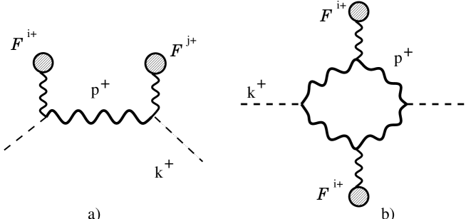
Figure 1: Tree (a) and one-loop (b) contributions to $\chi$ to quadratic order in $\rho$. Wavy lines with a blob denote insertions of the electric background field ${\cal F}^{+i}\,$; the thick internal wavy lines are propagators of the semi-fast gluons; the external dotted lines carry soft momenta, and couple to the fields $\delta A^{-}$.

To gain some more intuition, let us use as an example the contributions to $\delta\rho_{a}$ coming from the Yang-Mills piece of the action, $S_{YM}=\int d^{4}x(-F_{\mu\nu}^{2}/4)$ :

$$\delta\rho_{a}(x)\big{|}_{YM}\,=\,2gf^{abc}{\cal F}^{+i}_{b}(\vec{x})a^{i}_{c}(x)+gf^{abc}(\partial^{+}a_{b}^{i}(x))a_{c}^{i}(x).$$ (3.18)

(The additional contributions to $\delta\rho_{a}$, coming from $S_{W}$, will be presented in Sect. 4.3.) The first term in the r.h.s. is linear in the quantum fluctuations $a^{i}$ and in the electric background field ${\cal F}^{+i}$ (this is kinematically allowed because the semi-fast longitudinal momentum can flow from $a^{i}$ to ${\cal F}^{+i}$). It is only this term that contributes to $\hat{\chi}$ to leading order in $\alpha_{s}$. Indeed, it generates tree diagrams like the one depicted in Fig. 1.a, where the internal line represents the propagator $\langle a^{i}a^{j}\rangle$ of the semi-fast gluons, and the soft external legs couple to the fields $\delta A^{-}_{a}\/$. Physically, this diagram describes the emission of an on-shell, or real, semi-fast gluon by the classical source, which is a radiative correction to the direct emission of the soft field. This diagram will be evaluated in Sect. 5.2, but it is clear by power counting that it is of O$(\alpha_{s}\rho\rho)$. By contrast, one-loop diagrams which are of the same order in $\rho$ are necessarily of higher order in $g$, and thus negligible for the present purposes. [An exemple of such a diagram, of O$(\alpha_{s}^{2}\rho\rho)$, is shown in Fig. 1.b; this is generated by the second piece, quadratic in $a^{i}$, in the r.h.s. of eq. (3.18).]

When computing ${\cal G}(\vec{x},\vec{y})$, eq. (3.13), to LLA, the temporal non-locality in $\hat{\chi}$ can be ignored. To see this, consider eq. (3.15) with $x^{+}=y^{+}$ and $\langle\delta J^{\mu}\delta J^{\nu}\rangle$ replaced by $\hat{\chi}$. Since the external lines $G_{R}$ and $G_{A}$ are soft ($k^{+}\mathrel{\hbox to0.0pt{\raise 2.20013pt\hbox{$<$}\hss}{\lower 2.20013pt\hbox{$\sim$}}}b\Lambda^{+}$), the typical energy scale which controls the non-localities $x^{+}-z^{+}$ and $x^{+}-u^{+}$ (and therefore also $z^{+}-u^{+}$) is $k^{-}\equiv Q_{\perp}^{2}/2k^{+}\mathrel{\hbox to0.0pt{\raise 2.20013pt\hbox{$>$}\hss}{\lower 2.20013pt\hbox{$\sim$}}}\Lambda^{-}/b$ (cf. eq. (3.11)). This is much larger than the typical energy $p^{-}\ll\Lambda^{-}/b$ of the semi-fast gluons contributing to $\hat{\chi}$. Therefore, one can neglect the evolution of $\delta\rho$ during the small time interval $z^{+}-u^{+}\mathrel{\hbox to0.0pt{\raise 2.20013pt\hbox{$<$}\hss}{\lower 2.20013pt\hbox{$\sim$}}}b/\Lambda^{-}$, and replace $\hat{\chi}(z^{+}-u^{+})$ by its equal-time limit, which is independent of time:

$$\,\hat{\chi}(\vec{z},\vec{u})\,\equiv\,\hat{\chi}(z^{+}=u^{+},\vec{z},\vec{u})\,\equiv\,\alpha_{s}\ln{1\over b}\,\,\chi(\vec{z},\vec{u})\,.$$ (3.19)

As indicated above, it is only after taking the equal-time limit inside $\hat{\chi}$ that the logarithmic enhancement becomes manifest. The integrations over $z^{+}$ and $u^{+}$ then set $p^{-}=0$ in both external propagators, thus finally yielding

$$\langle\delta A^{i}(x^{+},\vec{x})\delta A^{j}(x^{+},\vec{y})\rangle\approx\int d^{3}\vec{z}\int d^{3}\vec{u}\,G^{\,i-}(\vec{x},\vec{z},p^{-}=0)\,\hat{\chi}(\vec{z},\vec{u})\,G^{\,-j}(\vec{u},\vec{y},p^{-}=0),\,\,\,$$ (3.20)

where we have omitted the subscripts $R$ and $A$ on the propagators since the boundary conditions in time become irrelevant as $p^{-}=0$. In particular, since $G^{--}=0$ for $p^{-}=0$, the two-point functions involving $\delta A^{-}_{a}$ (like $\langle\delta A^{-}\delta A^{-}\rangle$) vanish to LLA.

We now consider the induced mean field $\delta{\cal A}^{\mu}$, which can be obtained by solving eq. (3.5) to the order of interest:

$$0\,=\,\left\langle{\delta S\over\delta A^{\mu}_{a}(x)}\bigg{|}_{{\cal A}+\delta A+a}\right\rangle\Bigg{|}_{\langle a\rangle=0}\,\approx\,{\delta^{2}S\over\delta A^{\mu}_{a}(x)\delta A^{\nu}_{b}(y)}\bigg{|}_{{\cal A}}\delta{\cal A}_{b}^{\nu}(y)\,-\,{\cal J}_{\mu}^{\,a}(\vec{x}),$$ (3.21)

with an induced current:

$${\cal J}_{\mu}^{\,a}(\vec{x})\equiv-\,{1\over 2}\,{\delta^{3}S\over\delta A^{\mu}_{a}(x)\delta A^{\nu}_{b}(y)\delta A^{\lambda}_{c}(z)}\bigg{|}_{{\cal A}}\biggl{(}\Bigl{\langle}a^{\nu}_{b}(y)a^{\lambda}_{c}(z)\Bigr{\rangle}+\Bigl{\langle}\delta A^{\nu}_{b}(y)\delta A^{\lambda}_{c}(z)\Bigr{\rangle}\biggr{)}\,,$$ (3.22)

which involves two types of contributions: (a) A piece proportional to the 2-point function $\langle a^{\nu}a^{\lambda}\rangle$ of the semi-fast gluons, and (b) a second piece involving the induced correlator $\langle\delta A^{\nu}\delta A^{\lambda}\rangle$ of the soft fields, as given by eq. (3.15). Let us explain this in more detail:

(a) The first piece is the expectation value $\langle\delta J^{\mu}_{a}\rangle$ of the current (3.2.1). Once again, only the $\mu=+$ component, i.e., the induced color charge density :

$$\,\hat{\sigma}_{a}(\vec{x})\,\equiv\,\langle\delta\rho_{a}(x)\rangle\,,$$ (3.23)

matters to LLA: $\hat{\sigma}={\rm O}\bigl{(}\alpha_{s}\ln(1/b)\rho\bigr{)}$. In Fig. 2.a we show a diagram contributing to $\hat{\sigma}\/$ at lowest order in $\rho\,$; this is obtained by evaluating $gf^{abc}\langle(\partial^{+}a_{b}^{i})a_{c}^{i}\rangle$ to linear order in $\rho$ (cf. eq. (3.18)), and will be computed in Sect. 5.1. Note that the classical source $\rho$ is represented here as a continuous line; this is to suggest the physical origin of $\rho$ (namely, fast partons moving on straight line trajectories at the speed af light), and also the fact that its coupling to the semi-fast gluons is non-local in time (cf. Sect. 4.1).

(b) To LLA, the second piece in eq. (3.22) involves only the transverse field correlator $\langle\delta A^{i}\delta A^{j}\rangle$, which is proportional to $\hat{\chi}$ (cf. eq. (3.20)). We denote this as:

$$\delta{\cal J}_{\mu}\,\equiv\,-\,{1\over 2}\,{\delta^{3}S\over\delta A^{\mu}\delta A^{i}\delta A^{j}}\bigg{|}_{{\cal A}}\Bigl{(}G^{i-}\hat{\chi}\,G^{-j}\Bigr{)}.$$ (3.24)

This is of order $g\hat{\chi}\sim g\alpha_{s}\ln(1/b)\rho\rho\,$; thus, in the saturation regime where $g\rho\sim 1$, it is as large as the induced charge $\hat{\sigma}$.

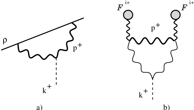
Figure 2: Contributions to the induced current to low orders in $\rho$. (a) A contribution to $\sigma_{a}\,$; the continuous line represents the classical source $\rho$. (b) A contribution to $\delta{\cal J}^{\mu}_{a}\,$; the thick internal line, with momentum $p^{+}$, is the propagator $\langle a^{i}a^{i}\rangle$ of the semi-fast gluons; the other, thiner, internal lines are the propagators $G^{i-}$ and $G^{-i}$ of the soft fields.

By using Fig. 1.a for $\hat{\chi}$, we obtain the contribution to $\delta{\cal J}_{\mu}$ depicted in Fig. 2.b, which should be compared to Fig. 2.a for $\hat{\sigma}$ : The logarithm $\ln(1/b)$ in the latter is generated by the integration over the internal $p^{+}$ momentum, which is restricted to the strip (3.8). By contrast, in Fig. 2.b the loop momentum is soft, but the propagator $\langle\delta A^{i}\delta A^{j}\rangle$ is itself of order $\alpha_{s}\ln(1/b)$, since proportional to $\hat{\chi}$. Thus, the logarithm is now generated by the subintegral giving $\hat{\chi}$. Note that, while $\hat{\sigma}$ describes the direct polarization of the semi-fast gluons, $\delta{\cal J}^{\mu}$ is rather an indirect effect of the latter, which induce a current after first modifying the propagator of the soft fields.

To summarize, ${\cal J}^{\mu}=\delta^{\mu+}\hat{\sigma}+\delta{\cal J}^{\mu}\,$. As we shall verify in Sect. 3.3, where $\delta{\cal J}^{\mu}$ will be constructed explicitly, the current ${\cal J}^{\mu}$ is covariantly conserved, ${\cal D}_{\mu}{\cal J}^{\mu}=0$, as necessary for the mean field equation (3.21) to be well defined. (Here, ${\cal D}_{\mu}\equiv\partial_{\mu}-ig{\cal A}_{\mu}$ is the covariant derivative constructed with the tree-level background field.) Since ${\cal J}^{\mu}$ is independent of time, the LC-gauge solution to eq. (3.21) is of the form (cf. Sect. 2.3):

$$\delta{\cal A}^{+}_{a} = \delta{\cal A}^{-}_{a}\,=\,0\,,$$

$$\delta{\cal A}^{i}_{a}(\vec{x}) = \int d^{3}\vec{y}\,\,G_{ab}^{\,i\nu}(\vec{x},\vec{y},p^{-}=0)\,{\cal J}_{\nu}^{\,b}(\vec{y}).$$ (3.25)

At this stage, the gluon density in eq. (3.13) can be compactly written as follows:

$${\cal G}(\vec{x},\vec{y})={\cal A}^{i}_{\vec{x}}{\cal A}^{i}_{\vec{y}}+(G^{\,i\nu}{\cal J}_{\nu})_{\vec{x}}\,{\cal A}^{i}_{\vec{y}}+{\cal A}^{i}_{\vec{x}}\,(G^{\,i\nu}{\cal J}_{\nu})_{\vec{y}}+(G^{\,i-}\hat{\chi}\,G^{\,-i})_{\vec{x}\,\vec{y}}\,.$$ (3.26)

The logarithmic enhancement is implicit in $\hat{\sigma}$ (which enters ${\cal J}^{\mu}$) and $\hat{\chi}$. In fact, to LLA, the induced charge $\hat{\sigma}(\vec{x})$ can be replaced in eq. (3.26) with a two-dimensional charge density localized at $x^{-}=0$ :

$$\hat{\sigma}_{a}(\vec{x}) \to \delta(x^{-})\,\alpha_{s}\ln{1\over b}\,\sigma_{a}({x}_{\perp}),$$ (3.27)

where

$$\alpha_{s}\ln{1\over b}\,\sigma_{a}({x}_{\perp})\,\equiv\,\int dx^{-}\,\hat{\sigma}_{a}(x^{-},x_{\perp})$$ (3.28)

is the effective color charge density in the transverse plane. As shown by the last equality, the logarithmic enhancement becomes manifest only after integrating over $x^{-}$.

To understand this last operation, recall the relevant longitudinal scales: $\sigma_{a}(\vec{x})$ is the color charge induced by the semi-fast gluons, and it spreads over longitudinal distances $1/\Lambda^{+}\mathrel{\hbox to0.0pt{\raise 2.20013pt\hbox{$<$}\hss}{\lower 2.20013pt\hbox{$\sim$}}}x^{-}\mathrel{\hbox to0.0pt{\raise 2.20013pt\hbox{$<$}\hss}{\lower 2.20013pt\hbox{$\sim$}}}1/b\Lambda^{+}$ (this will be verified by the explicit calculations in Sect. 5.1 and Paper II). Thus, $\sigma_{a}$ sits further away from the light-cone than the original source $\rho_{a}$ (which, we recall, has support at $0\mathrel{\hbox to0.0pt{\raise 2.20013pt\hbox{$<$}\hss}{\lower 2.20013pt\hbox{$\sim$}}}x^{-}\mathrel{\hbox to0.0pt{\raise 2.20013pt\hbox{$<$}\hss}{\lower 2.20013pt\hbox{$\sim$}}}1/\Lambda^{+}$), but it is still very close to $x^{-}=0$ on the resolution scale of the soft fields $\delta A^{i}$. In convolutions like

$$(G^{\,i-}\hat{\sigma})_{\vec{x}}\equiv\int d^{3}\vec{y}\,G^{\,i-}(\vec{x},\vec{y})\,\hat{\sigma}(\vec{y}),$$ (3.29)

the integral over $y^{-}$ runs typically over large distances $y^{-}\gg 1/b\Lambda^{+}$, where it is indeed legitimate to replace $\hat{\sigma}(\vec{x})$ as shown in eq. (3.27).

Since eqs. (3.20) and (3.24) involve similar convolutions, there too one can replace

$$\hat{\chi}_{ab}(\vec{x},\vec{y}) \to \delta(x^{-})\,\alpha_{s}\ln{1\over b}\,\chi_{ab}(x_{\perp},y_{\perp})\,\delta(y^{-}),$$

$$\alpha_{s}\ln{1\over b}\,\chi_{ab}(x_{\perp},y_{\perp}) \equiv \int dx^{-}\int dy^{-}\,\hat{\chi}_{ab}(\vec{x},\vec{y}).$$ (3.30)

In fact, $\hat{\chi}$ turns out to be even more localized than $\hat{\sigma}\,$: Indeed, $\hat{\chi}$ is explicitly proportional to the tree-level source $\rho$ and/or electric field ${\cal F}^{+i}$, since it is generated by vertices which have this property (like the first term in the r.h.s. of eq. (3.18); see also Fig. 1.a). Thus, $\hat{\chi}(\vec{x},\vec{y})$ has support at $0\mathrel{\hbox to0.0pt{\raise 2.20013pt\hbox{$<$}\hss}{\lower 2.20013pt\hbox{$\sim$}}}x^{-},y^{-}\mathrel{\hbox to0.0pt{\raise 2.20013pt\hbox{$<$}\hss}{\lower 2.20013pt\hbox{$\sim$}}}1/\Lambda^{+}$, like the original source $\rho$.

The previous considerations show that the longitudinal and temporal structure of the quantum corrections do not matter when computing soft correlation functions: when “seen” by the soft fields, the (semi)fast gluons appear as a static color charge localized near the light-cone. This is consistent with the physical picture in Sect. 2.1, and also clarifies its limitations: This picture holds only to LLA, which is the accuracy to which we have a strong separation of scales. To this accuracy, only the one-point ($\hat{\sigma}$) and two-point ($\hat{\chi}$) correlations of the quantum charge $\delta\rho$ must be kept (cf. Sect. 4.3 below). This is why, for matching purposes, it is enough to consider the two-point function $\langle A^{i}A^{i}\rangle$, as we do here. This is finally given by:

$${\cal G}(\vec{x},\vec{y})\,\approx\,{\cal A}^{i}_{\vec{x}}{\cal A}^{i}_{\vec{y}}\,+\,\alpha_{s}\ln(1/b)\Bigl{\{}(G^{\,i\nu}{\cal J}_{\nu})_{\vec{x}}\,{\cal A}^{i}_{\vec{y}}+{\cal A}^{i}_{\vec{x}}\,(G^{\,i\nu}{\cal J}_{\nu})_{\vec{y}}+(G^{\,i-}\chi\,G^{\,-i})_{\vec{x}\,\vec{y}}\Bigr{\}},$$ (3.31)

where the logarithmic factor $\ln(1/b)$ is now explicit. After averaging over $\rho$ with weight function $W_{\Lambda}[\rho]$, eq. (3.31) gives the gluon density at the scale $b\Lambda^{+}$, as computed in Theory I to LLA. By construction, this must be the same as the gluon density in Theory II at tree-level. That is, the following equality must hold:

$$\langle{\cal A}^{i}_{\vec{x}}{\cal A}^{i}_{\vec{y}}\rangle_{b\Lambda}=\langle{\cal A}^{i}_{\vec{x}}{\cal A}^{i}_{\vec{y}}\rangle_{\Lambda}+\alpha_{s}\ln(1/b)\Bigl{\langle}(G^{\,i\nu}{\cal J}_{\nu})_{\vec{x}}\,{\cal A}^{i}_{\vec{y}}+{\cal A}^{i}_{\vec{x}}\,(G^{\,i\nu}{\cal J}_{\nu})_{\vec{y}}+(G^{\,i-}\chi\,G^{\,-i})_{\vec{x}\,\vec{y}}\Bigr{\rangle}_{\Lambda},\,\,\,\,$$ (3.32)

where, e.g.,

$$\langle{\cal A}^{i}_{\vec{x}}{\cal A}^{i}_{\vec{y}}\rangle_{\Lambda}\,\equiv\,\int{\cal D}\rho\,\,W_{\Lambda}[\rho]\,\,{\cal A}_{a}^{i}({\vec{x}}){\cal A}_{a}^{i}({\vec{y}})\,,$$ (3.33)

together with a similar definition for $\langle{\cal A}^{i}{\cal A}^{i}\rangle_{b\Lambda}$ in terms of $W_{b\Lambda}$. Eq. (3.32) is the evolution equation for the gluon density, and can be used to derive the evolution $W_{\Lambda}[\rho]\,\to\,W_{b\Lambda}[\rho]$ of the classical weight function, as it will be explained shortly.

To avoid cumbersome notations, in what follows we shall not always distinguish between $\hat{\sigma}$ and $\sigma$, or between $\hat{\chi}$ and $\chi$; these quantities differ just by their arguments and by a factor of $\alpha_{s}\ln(1/b)$ (cf. eqs. (3.27)–(3.28) and (3.2.1)), which will be written down explicitly whenever needed.

3.2.2 Tree-level calculation in Theory II

In this subsection, the evolution equation for $W_{\tau}[\rho]$ will be established in two steps: First, we shall show that the quantum corrections described previously can be generated by adding a Gaussian “noise term” to the Yang Mills equation (2.2). Then, we shall absorb this noise term into a redefinition of the classical source and weight function.

Our starting point is the following Yang Mills equation:

$$[D_{\nu},F^{\nu\mu}]_{a}\,=\,\delta^{\mu+}(\rho_{a}(\vec{x})+\nu_{a}(\vec{x})),$$ (3.34)

which in addition to eq. (2.2) contains a random source $\nu_{a}(\vec{x})$ (the “noise term”) chosen such as to generate, via the solution to eq. (3.34), the same two-point function $\langle A^{i}A^{i}\rangle$ as obtained in Theory I after including the quantum corrections (cf. eq. (3.31)). Thus, $\nu_{a}$ plays the role of the fluctuating charge $\delta\rho_{a}$ of the semi-fast gluons. Based on this analogy, we take $\nu_{a}$ to be static and have the same non-trivial correlators as $\delta\rho_{a}$, namely (with $\langle\cdots\rangle_{\nu}$ denoting the average over $\nu$) :

$$\,\langle\nu_{a}(\vec{x})\rangle_{\nu}\,=\,\sigma_{a}(\vec{x}),\qquad\langle\nu_{a}(\vec{x})\nu_{b}(\vec{y})\rangle_{\nu}\,=\,\chi_{ab}(\vec{x},\vec{y}).$$ (3.35)

From the previous subsection, we recall that the precise longitudinal structure of $\sigma$ and $\chi$ does not matter for the calculation of soft correlations. As we shall shortly discover, to a large extent this is also true for the evolution equation, which involves only the integrated densities $\sigma_{a}(x_{\perp})$ and $\chi_{ab}(x_{\perp},y_{\perp})$, eqs. (3.28) and (3.2.1). Still, for this equation to be well defined, it will be important to recall that the induced charge $\sigma_{a}(\vec{x})$ has a longitudinal support which is separated from that of the original source $\rho$ (cf. the discussion after eq. (3.28)). This property is relevant here since the solution to the classical equation (3.34) involves the color source via path-ordered exponentials in $x^{-}$, cf. Sect. 2.3. To keep trace of that, and for consistency with the first equation (3.35), we choose $\nu_{a}(\vec{x})$ to have support in the range $1/\Lambda^{+}\mathrel{\hbox to0.0pt{\raise 2.20013pt\hbox{$<$}\hss}{\lower 2.20013pt\hbox{$\sim$}}}x^{-}\mathrel{\hbox to0.0pt{\raise 2.20013pt\hbox{$<$}\hss}{\lower 2.20013pt\hbox{$\sim$}}}1/b\Lambda^{+}$, so like $\sigma$.

We first verify that the classical stochastic problem in eqs. (3.34)–(3.35) generates the same correlator $\langle A^{i}A^{i}\rangle$ as the quantum problem in Sect. 3.2.1. The solution $A^{\mu}[\rho,\nu]$ to eq. (3.34) can be read off Sect. 2.3: if ${\cal A}^{i}[\rho]$ is the solution (2.18) to eq. (2.2), then, clearly,

$$A^{\mu}[\rho,\nu](x)\,=\,\delta^{\mu i}{\cal A}^{i}[\rho+\nu](\vec{x}).$$ (3.36)

For fixed $\rho$, this is a random variable whose correlations can be obtained by expanding in powers of $\nu$, and then averaging over $\nu$ with the help of eq. (3.35). To the order of interest, we need the expansion of (3.36) to quadratic order (below, ${\cal A}^{i}_{x}\equiv{\cal A}^{i}_{a}[\rho](\vec{x})$) :

$${\cal A}^{i}_{x}[\rho+\nu]\,\approx\,{\cal A}^{i}_{x}[\rho]\,+\,{\delta{\cal A}^{i}_{x}\over\delta\rho_{y}}\bigg{|}_{\rho}\nu_{y}\,+\,{1\over 2}\,{\delta^{2}{\cal A}^{i}_{x}\over\delta\rho_{y}\delta\rho_{z}}\bigg{|}_{\rho}\nu_{y}\nu_{z}\,\equiv\,{\cal A}^{i}_{x}[\rho]\,+\,\delta{A}^{i}_{x}[\rho,\nu]\,.$$ (3.37)

Indeed, after averaging over $\nu$, both the linear and the quadratic term will contribute to order $\alpha_{s}\ln(1/b)$, while the terms neglected in eq. (3.37) would be of higher order. The classical two-point correlation function is then obtained as:

$$\,\langle{\cal A}^{i}_{x}[\rho+\nu]\,{\cal A}^{i}_{y}[\rho+\nu]\rangle_{\nu}\,=\,{\cal A}^{i}_{x}{\cal A}^{i}_{y}\,+\,\langle\delta{A}^{i}_{x}\rangle_{\nu}{\cal A}^{i}_{y}\,+\,{\cal A}^{i}_{x}\langle\delta{A}^{i}_{y}\rangle_{\nu}\,+\,\langle\delta{A}^{i}_{x}\delta{A}^{i}_{y}\rangle_{\nu}\,,$$ (3.38)

where, to the order of interest,

$$\langle\delta{A}^{i}_{x}\rangle_{\nu} = {\delta{\cal A}^{i}_{x}\over\delta\rho_{y}}\bigg{|}_{\rho}\sigma(y)\,+\,{1\over 2}\,{\delta^{2}{\cal A}^{i}_{x}\over\delta\rho_{y}\delta\rho_{z}}\bigg{|}_{\rho}\chi(y,z),$$

$$\langle\delta{A}^{i}_{x}\delta{A}^{i}_{y}\rangle_{\nu} = {\delta{\cal A}^{i}_{x}\over\delta\rho_{z}}\bigg{|}_{\rho}\chi(z,u)\,{\delta{\cal A}^{i}_{y}\over\delta\rho_{u}}\,.$$ (3.39)

These classical correlators coincide with the corresponding quantum corrections $\delta{\cal A}^{i}$, eq. (3.2.1), and $\langle\delta A^{i}\delta A^{i}\rangle$, eq. (3.20), as we demonstrate now:

For the two-point function, one can use the following identity, to be derived shortly,

$${\delta{\cal A}^{i}_{x}\over\delta\rho_{y}}\bigg{|}_{\rho}\,\equiv\,G^{\,i-}(\vec{x},\vec{y},p^{-}=0),$$ (3.40)

to conclude that the expression (3.2.2) for $\langle\delta{A}^{i}\delta{A}^{i}\rangle_{\nu}$ is indeed the same as eq. (3.20) for $\langle\delta A^{i}\delta A^{i}\rangle$. Eq. (3.40) can be proven by noticing that, to linear order in $\nu$, $\delta{A}^{i}\approx G^{\,i-}\nu$, which must be the same as the linear-order term in eq. (3.37).

Eq. (3.40) also shows that the first term in the r.h.s. of eq. (3.2.2) for $\langle\delta{A}^{i}\rangle_{\nu}$ is the same as $G^{\,i-}\sigma$, which is one of the contributions to $\delta{\cal A}^{i}$ in eq. (3.2.1). The other contribution, involving $\delta{\cal J}^{\mu}_{a}$, can be similarly identified with the term proportional to $\chi$ in eq. (3.2.2). More rapidly, the equality between $\langle\delta{A}^{i}\rangle_{\nu}$ and $\delta{\cal A}^{i}$ can be established by showing that they both satisfy the same equation of motion. In the case of $\langle\delta{A}^{i}\rangle_{\nu}$, this is obtained by averaging eq. (3.34) over $\nu$, and can be rewritten as:

$$\left\langle{\delta S_{YM}\over\delta A^{\mu}_{a}}\bigg{|}_{{\cal A}+\delta A}\right\rangle_{\nu}\,=\,\delta_{\mu-}(\rho_{a}+\sigma_{a}),$$ (3.41)

where $S_{YM}$ is the Yang-Mills action. For $\delta{\cal A}^{i}$, the corresponding equation is rather (3.21), which is equivalent to:

$$\left\langle{\delta S\over\delta A^{\mu}_{a}}\bigg{|}_{{\cal A}+\delta A}\right\rangle\,\approx\,\delta_{\mu-}\sigma_{a}.$$ (3.42)

Since ${\cal A}^{-}=\delta A^{-}=0$, this is formally similar to eq. (3.41). The final identification between these two equations then follows after recalling that the corresponding two-point functions $\langle\delta A^{i}\delta A^{i}\rangle$ (which enter both eq. (3.41) and eq. (3.42)) are also the same.

To summarize, the classical two-point function (3.38) coincide with the corresponding quantum function ${\cal G}(\vec{x},\vec{y})$, eq. (3.31). This allows us to write:

$$\,{\cal G}(\vec{x},\vec{y})\,=\,\langle{\cal A}^{i}_{x}[\rho+\nu]\,{\cal A}^{i}_{y}[\rho+\nu]\rangle_{\nu}\,\equiv\,\int{\cal D}\nu\,{\cal W}[\nu\,;\rho]\,\,{\cal A}^{i}_{x}[\rho+\nu]\,{\cal A}^{i}_{y}[\rho+\nu]\,,$$ (3.43)

where the second equality is just a rewritting of the average over $\nu$ as a functional integral with the Gaussian weight function:

$$\,{\cal W}[\nu\,;\rho]\,\equiv\,{\rm e}^{-{1\over 2}{\rm Tr}\ln\chi}\,\,{\rm exp}\left\{-{1\over 2}\,(\nu-\sigma)_{x}\chi_{x,y}^{-1}(\nu-\sigma)_{y}\right\}.$$ (3.44)

(This depends upon $\rho$ via $\chi$ and $\sigma$.) After also averaging over $\rho$, with weight function $W_{\Lambda}[\rho]$, eq. (3.43) must be the same as the gluon density generated in Theory II at tree-level (cf. eq. (3.32)). This requires:

$$\int{\cal D}\rho\,\,W_{b\Lambda}[\rho]\,\,{\cal A}_{x}^{i}[\rho]{\cal A}_{y}^{i}[\rho]\,=\,\int{\cal D}\rho\,\,W_{\Lambda}[\rho]\int{\cal D}\nu\,{\cal W}[\nu\,;\rho]\,\,{\cal A}^{i}_{x}[\rho+\nu]\,{\cal A}^{i}_{y}[\rho+\nu]\,,$$ (3.45)

which is satisfied provided

$$W_{b\Lambda}[\rho]\,=\,\int{\cal D}\nu\,W_{\Lambda}[\rho-\nu]\,{\cal W}[\nu\,;\rho-\nu]\,.$$ (3.46)

This is a functional recurrency formula for $W[\rho]$, whose r.h.s. can be expanded as follows:

$$W_{\Lambda}[\rho-\nu]\,{\cal W}[\nu\,;\rho-\nu]\,\approx\,\left(1\,-\,\nu_{x}\,{\delta\over\delta\rho_{x}}\,+\,{1\over 2}\,\nu_{x}\,\nu_{y}\,{\delta^{2}\over\delta\rho_{x}\delta\rho_{y}}\right)W_{\Lambda}[\rho]\,{\cal W}[\nu\,;\rho]\,,$$ (3.47)

and then integrated over $\nu$ to give, to the order of interest,

$$W_{b\Lambda}[\rho]\,-\,W_{\Lambda}[\rho]\,=\,-\,{\delta\over\delta\rho_{x}}\,[W_{\Lambda}\sigma_{x}]\,+\,{1\over 2}\,{\delta^{2}\over\delta\rho_{x}\delta\rho_{y}}[W_{\Lambda}\chi_{xy}].$$ (3.48)

A priori, the convolutions in the r.h.s. of eq. (3.48) involve three-dimensional integrals, like

$${\delta\over\delta\rho_{x}}\,[W_{\Lambda}\sigma_{x}]\,\equiv\,\int d^{3}{\vec{x}}\,{\delta\over\delta\rho_{a}(\vec{x})}\,\Bigl{[}W_{\Lambda}\sigma_{a}(\vec{x})\Bigr{]}.$$ (3.49)

Recall, however, that $\sigma$ is distributed over distances $1/\Lambda^{+}\mathrel{\hbox to0.0pt{\raise 2.20013pt\hbox{$<$}\hss}{\lower 2.20013pt\hbox{$\sim$}}}x^{-}\mathrel{\hbox to0.0pt{\raise 2.20013pt\hbox{$<$}\hss}{\lower 2.20013pt\hbox{$\sim$}}}1/b\Lambda^{+}$, and that the logarithmic enhancement is seen only after integration over $x^{-}$, cf. eq. (3.28). In the limit $b\to 1$, in which we are eventually interested, eq. (3.49) can be replaced with

$${\delta\over\delta\rho_{x}}\,[W_{\Lambda}\sigma_{x}]\,=\,\alpha_{s}\ln{1\over b}\,\int d^{2}{x_{\perp}}\,{\delta\over\delta\rho_{a}(x^{-}_{\Lambda},x_{\perp})}\,\Bigl{[}W_{\Lambda}\sigma_{a}(x_{\perp})\Bigr{]},$$ (3.50)

where the functional derivative is to be evaluated at $x^{-}_{\Lambda}\equiv 1/\Lambda^{+}$.

It is convenient to introduce the rapidity variable $\tau\equiv\ln(P^{+}/\Lambda^{+})=\ln(1/x)$, where $P^{+}$ is the total longitudinal momentum of the hadron, and $x$ is Bjorken’s $x$ (cf. Sect. 2.1). Then, $\ln(P^{+}/b\Lambda^{+})=\tau+\Delta\tau$, with $\Delta\tau\equiv\ln(1/b)$. After also renoting $W_{\Lambda}\equiv W_{\tau}$, $W_{b\Lambda}\equiv W_{\tau+\Delta\tau}$, and $x^{-}_{\Lambda}=1/\Lambda^{+}\equiv x^{-}_{\tau}$, eq. (3.48) is rewritten as

$$W_{\tau+\Delta\tau}[\rho]-W_{\tau}[\rho]\,=\,\alpha_{s}\Delta\tau\left\{{1\over 2}{\delta^{2}\over{\delta\rho_{\tau}(x)\delta\rho_{\tau}(y)}}[W_{\tau}\chi_{xy}]-{\delta\over{\delta\rho_{\tau}(x)}}[W_{\tau}\sigma_{x}]\right\}\,,$$ (3.51)

where $\rho_{\tau}(x_{\perp})\equiv\rho(x^{-}_{\tau},x_{\perp})$, and the convolutions are now to be understood as two dimensional integrals, cf. eq. (3.50). For instance:

$${\delta\over\delta\rho_{\tau}(x)}\,[W_{\tau}\sigma_{x}]\,=\,\int d^{2}{x_{\perp}}\,{\delta\over\delta\rho_{a}(x^{-}_{\tau},x_{\perp})}\,\Bigl{[}W_{\tau}\sigma_{a}(x_{\perp})\Bigr{]}.$$ (3.52)

According to eqs. (3.51)–(3.52), the evolution from $W_{\tau}[\rho]$ to $W_{\tau+\Delta\tau}[\rho]$ is due to changes in $\rho$ within the rapidity interval $(\tau,\tau+\Delta\tau)$, where the quantum corrections are located.

Note that the variable $\tau$ in the above equations acts simultaneously as a momentum rapidity [$\tau=\ln(P^{+}/\Lambda^{+})$], and as a space-time rapidity [$\tau=\ln(x^{-}_{\tau}/x^{-}_{0})$, with $x^{-}_{0}$ some arbitrary scale of reference; e.g., $x^{-}_{0}=1/P^{+}$]. This is so since the support of the quantum corrections is correlated to the longitudinal momenta of the modes which have been integrated out. These equations suggest a space-time picture of the quantum evolution where the color source is built up by adding contributions in successive layers of (space-time) rapidity, from $x^{-}=0$ up.

By taking the limit $\Delta\tau\equiv\ln(1/b)\to 0$, we finally obtain a functional differential equation for the evolution of the weight function with $\tau\equiv\ln(1/x)\/$:

$${\partial W_{\tau}[\rho]\over{\partial\tau}}\,=\,\alpha_{s}\left\{{1\over 2}{\delta^{2}\over{\delta\rho_{\tau}(x)\delta\rho_{\tau}(y)}}[W_{\tau}\chi_{xy}]-{\delta\over{\delta\rho_{\tau}(x)}}[W_{\tau}\sigma_{x}]\right\}\,.$$ (3.53)

This renormalization group equation (RGE) has been originally derived in Ref. [11], although its longitudinal structure — i.e., the fact that the functional differentiations are to be taken with respect to the color source in the highest bin of rapidity $(\tau,\tau+d\tau)$ — has not been recognized there. (In Ref. [11] the differentiations are rather taken w.r.t. the integrated charge density $\rho(x_{\perp})\equiv\int dx^{-}\rho(\vec{x})$.) To understand the importance of this structure, recall from Sect. 2.3 that the classical solution ${\cal A}^{i}[\rho]$ — and therefore also the quantum corrections $\sigma$ and $\chi$, which are functionals of ${\cal A}^{i}$ [32] — depends upon $\rho$ via Wilson lines in $x^{-}$ (cf. eq. (2.29)). Thus, in evaluating eq. (3.53), we shall be led to differentiate [32]

$$V^{\dagger}(y_{\perp})\,\equiv\,{\rm P}\exp\left\{ig\int_{-\infty}^{x^{-}_{\tau}}dz^{-}\int d^{2}z_{\perp}\langle y_{\perp}|\,{-1\over\nabla^{2}_{\perp}}\,|z_{\perp}\rangle\,\tilde{\rho}_{a}(z^{-},z_{\perp})T^{a}\right\},$$ (3.54)

with respect to $\tilde{\rho}_{\tau}(x)$. Note the upper limit $x^{-}_{\tau}$ in the integral above: this occurs since the original source $\tilde{\rho}$ has support up to $x^{-}\simeq x^{-}_{\tau}$. Because of the path-ordering in $x^{-}$, the functional derivative of eq. (3.54) is as simple as a normal derivative:

$${\delta\over\delta\tilde{\rho}_{a}(x^{-}_{\tau},x_{\perp})}\,V^{\dagger}(y_{\perp})\,=\,ig\,\langle x_{\perp}|\,{-1\over\nabla^{2}_{\perp}}\,|y_{\perp}\rangle\,T^{a}\,V^{\dagger}(y_{\perp}).$$ (3.55)

By contrast, its derivative w.r.t. the integrated charge $\tilde{\rho}_{a}(x_{\perp})$ is not well defined.

Note also that the color source which appears in eqs. (3.54)–(3.55) is the covariant-gauge source $\tilde{\rho}_{a}$, and not the LC-gauge source $\rho_{a}$. It is only with respect to $\tilde{\rho}_{a}$ that we know the classical solution explicitly. This brings us to the necessity to rewrite the RGE (3.53) as an evolution equation for $W_{\tau}[\tilde{\rho}]$, which will shall do in the next subsection.

Let us conclude this subsection with a few remarks on eq. (3.53). This can be recognized as a functional Fokker-Planck equation [34], with $\tau$ playing the role of time. It describes diffusion in the functional space spanned by $\rho$, with ($\rho$-dependent) “drift velocity” $\alpha_{s}\sigma$ and “diffusion constant” $\alpha_{s}\chi$. (In this language, the recurrency formula (3.46) can be viewed as a functional Chapman-Kolmogorov equation [34].) Alternatively, eq. (3.53) is like a functional Schrödinger equation in imaginary “time” $\tau$. It can be transformed into an hierarchy of ordinary differential equations for the correlation functions $\langle\rho\rho\cdots\rho\rangle_{\tau}$ generated by $W_{\tau}[\rho]\,$. For instance, by multiplying it with $\rho(x)\rho(y)$ and functionally integrating over $\rho$, one obtains an evolution equation for the two-point function:

$${d\over{d\tau}}\,\Big{\langle}\rho_{a}(\vec{x})\rho_{b}(\vec{y})\Big{\rangle}_{\tau} = \alpha_{s}\,\Big{\langle}\delta(x^{-}-x^{-}_{\tau})\sigma_{a}(x_{\perp})\rho_{b}(\vec{y})\,+\,\delta(y^{-}-x^{-}_{\tau})\rho_{a}(\vec{x})\sigma_{b}(y_{\perp})$$ (3.56)

$$\,\,\,\,\,\,+\,\delta(x^{-}-x^{-}_{\tau})\delta(y^{-}-x^{-}_{\tau})\chi_{ab}(x_{\perp},y_{\perp})\Bigr{\rangle}_{\tau}\,,$$

where $\langle\cdots\rangle_{\tau}$ denotes the average over $\rho$ with weight function $W_{\tau}[\rho]\,$. For strong fields and sources, that is, in the saturation regime, this equation involves also the higher $n$-point correlators ($n\geq 3$), since $\sigma$ and $\chi$ are non-linear in $\rho$ [32]. But in the weak source limit, where the non-linear effects can be neglected, eq. (3.56) closes at the level of the two-point functions, and becomes equivalent to the BFKL equation, as demonstrated in Ref. [10] (see also Sect. 5 below, and Paper II, where the BFKL equation will be recovered as the weak field limit of the general evolution equations).

3.3 Evolution equation with a covariant-gauge source

For the RGE (3.53) to be of practical use, its coefficients $\sigma$ and $\chi$ must be known explicitly in terms of the tree-level source $\rho$. This requires, in particular, an explicit expression for the classical solution ${\cal A}^{i}[\rho]$ (since $\sigma$ and $\chi$ are functionals of ${\cal A}^{i}$; cf. Sects. 4, 5 and Paper II). From Sect. 2.3, we know that such an explicit expression can be obtained if the light-cone gauge solution ${\cal A}^{i}$ is expressed in terms of the covariant gauge (COV-gauge) charge density $\tilde{\rho}$. This observation, together with the gauge invariance of the weight function ($W_{\Lambda}[\rho]=W_{\Lambda}[\tilde{\rho}]$), makes it more convenient to use $\tilde{\rho}$ as the classical source variable to be averaged over. In this subsection, we shall rewrite the RGE in this new variable. This is non-trivial since, as it will be explained shortly, the gauge rotation from $\rho$ to $\tilde{\rho}$ is itself subjected to quantum evolution.

Recall indeed that the definition of the COV-gauge depends upon the classical color source in the problem: For a given static source $\rho_{a}(\vec{x})$ in the LC-gauge, the COV-gauge is the gauge where the classical field generated by $\rho$ has just a plus component, $\tilde{A}^{\mu}=\delta^{\mu+}\alpha$, with $\alpha$ linearly related to $\tilde{\rho}$ (the COV-gauge version of $\rho$). Thus, if the classical source is modified by quantum corrections (say, from $\rho$ to $\rho+\nu$ in the LC gauge), then what we mean by “the covariant gauge” changes as well: This is now the gauge where the new classical field, as generated by the total charge $\rho+\nu$, has just a plus component, say $\bar{A}^{\mu}=\delta^{\mu+}\bar{\alpha}$, with $\bar{\alpha}$ linearly related to the COV-gauge source $\bar{\rho}+\bar{\nu}$. [Note that we denote with a tilde (a bar) quantities in the COV-gauge associated with $\rho$ (respectively, $\rho+\nu$).] Clearly, the rotation between the old and the new COV-gauges depends on $\nu$, and thus upon the quantum corrections. In what follows, we shall construct this rotation explicitly.

Recall first the classical solution corresponding to $\tilde{\rho}$, as constructed in Sect. 2.3. This is summarized in the following equations:

$$\,{\cal A}^{i}[\tilde{\rho}]\,(\vec{x}) = {i\over g}\,U(\vec{x})\,\partial^{i}U^{\dagger}(\vec{x}),$$

$$U^{\dagger}(x^{-},x_{\perp}) = {\rm P}\exp\left\{ig\int_{-\infty}^{x^{-}}dz^{-}\,{\alpha}(z^{-},x_{\perp})\right\},$$

$$-\nabla^{2}_{\perp}\alpha({\vec{x}}) = {\tilde{\rho}}(\vec{x})\,,$$ (3.57)

where $U^{\dagger}(\vec{x})$ is the gauge rotation from the LC-gauge to the original COV-gauge (cf. eq. (2.21)).

When the classical source changes from $\rho$ to $\rho+\nu$, the corresponding solution is obtained by replacing $\tilde{\rho}\rightarrow\bar{\rho}+\bar{\nu}$ in eqs. (3.3) :

$$\,{\cal A}^{i}[\bar{\rho}+\bar{\nu}]\,(\vec{x}) = {i\over g}\,\bar{U}(\vec{x})\,\partial^{i}\bar{U}^{\dagger}(\vec{x}),$$

$$\bar{U}^{\dagger}(x^{-},x_{\perp}) = {\rm P}\exp\left\{ig\int_{-\infty}^{x^{-}}dz^{-}\,\bar{\alpha}(z^{-},x_{\perp})\right\},$$

$$-\nabla^{2}_{\perp}\bar{\alpha} = \bar{\rho}+\bar{\nu}\,.$$ (3.58)

We write $\bar{U}^{\dagger}\equiv\delta U^{\dagger}\,U^{\dagger}$, with $\delta U^{\dagger}$ the gauge rotation from the original COV-gauge towards the new one. It turns out that this has a relatively simple expression in terms of $\bar{\nu}$.

To see this, we set $\bar{\alpha}=\alpha+\delta\alpha$, with $\alpha$ defined by the last equation (3.3) and $\delta\alpha$ proportional to $\nu$. These two fields have no overlap in the longitudinal direction: $\alpha$, like $\rho$, has support at $0\mathrel{\hbox to0.0pt{\raise 2.20013pt\hbox{$<$}\hss}{\lower 2.20013pt\hbox{$\sim$}}}x^{-}\mathrel{\hbox to0.0pt{\raise 2.20013pt\hbox{$<$}\hss}{\lower 2.20013pt\hbox{$\sim$}}}1/\Lambda^{+}$, while $\nu$, and therefore $\delta\alpha$, is rather localized at $1/\Lambda^{+}\mathrel{\hbox to0.0pt{\raise 2.20013pt\hbox{$<$}\hss}{\lower 2.20013pt\hbox{$\sim$}}}x^{-}\mathrel{\hbox to0.0pt{\raise 2.20013pt\hbox{$<$}\hss}{\lower 2.20013pt\hbox{$\sim$}}}1/b\Lambda^{+}$. Then, the path-ordered exponential in eq. (3.3) simply factorizes:

$$\,\bar{U}^{\dagger}(x^{-},x_{\perp})\,\equiv\,\delta U^{\dagger}(\vec{x})\,U^{\dagger}(\vec{x})\,\approx\,{\rm exp}\Bigl{\{}{ig\theta(x^{-}-x^{-}_{\tau})\delta{\alpha}(x_{\perp})}\Bigr{\}}\,U^{\dagger}(\vec{x})\,,$$ (3.59)

where $x^{-}_{\tau}=1/\Lambda^{+}$, $\delta{\alpha}(x_{\perp})\equiv\int dx^{-}\delta{\alpha}(\vec{x})$, and the approximate equality holds as $b\to 1$. In particular, within the support of $\rho$, $\bar{U}^{\dagger}$ reduces to $U^{\dagger}$, and therefore

$$\bar{\rho}\,=\,\bar{U}^{\dagger}\rho\bar{U}\,=\,U^{\dagger}\rho U\,=\,\tilde{\rho}.$$ (3.60)

Thus, remarkably, the original source $\tilde{\rho}$ is not affected by the supplementary gauge rotation $\delta U^{\dagger}$ induced by the quantum corrections. By using this property, and subtracting the equation satisfied by $\alpha$ from the equation for $\bar{\alpha}$, we deduce

$$-\nabla^{2}_{\perp}\delta{\alpha}(\vec{x})\,=\,\bar{\nu}(\vec{x})\,,$$ (3.61)

which shows that $\delta{\alpha}$ is linear in $\bar{\nu}$.

We are now in a position to reformulate the RGE by using the COV-gauge source as a variable. The analog of eq. (3.45) reads:

$$\int{\cal D}\tilde{\rho}\,\,W_{b\Lambda}[\tilde{\rho}]\,\,{\cal A}_{x}^{i}[\tilde{\rho}]{\cal A}_{y}^{i}[\tilde{\rho}]\,=\,\int{\cal D}\tilde{\rho}\,\,W_{\Lambda}[\tilde{\rho}]\int{\cal D}\bar{\nu}\,{\cal W}[\bar{\nu}\,;\tilde{\rho}]\,\,{\cal A}^{i}_{x}[\bar{\rho}+\bar{\nu}]\,{\cal A}^{i}_{y}[\bar{\rho}+\bar{\nu}]\,.$$ (3.62)

Note the assignments of tilde’s and bar’s in the r.h.s.: This is what we need since, first, $\tilde{\rho}$ is the COV-gauge source at tree-level, and, second, the classical solution corresponding to $\rho+\nu$ is the same functional of $\bar{\rho}+\bar{\nu}$ as the tree-level field in terms of $\tilde{\rho}$ (cf. eqs. (3.3) and (3.3)). By also using $\tilde{\rho}=\bar{\rho}$ (cf. eq. (3.60)), the r.h.s. can be rewritten as:

$$\int{\cal D}\bar{\rho}\,\,W_{\Lambda}[\bar{\rho}]\int{\cal D}\bar{\nu}\,{\cal W}[\bar{\nu}\,;\bar{\rho}]\,\,{\cal A}^{i}_{x}[\bar{\rho}+\bar{\nu}]\,{\cal A}^{i}_{y}[\bar{\rho}+\bar{\nu}]\,,$$ (3.63)

which leads to the following recurrency formula (compare to eq. (3.46)):

$$W_{b\Lambda}[\tilde{\rho}]\,=\,\int{\cal D}\bar{\nu}\,W_{\Lambda}[\tilde{\rho}-\bar{\nu}]\,{\cal W}[\bar{\nu}\,;\tilde{\rho}-\bar{\nu}]\,.$$ (3.64)

Thus, in this framework, it is natural to define the noise correlations directly for $\bar{\nu}$. We write (compare to eq. (3.35)):

$$\,\langle\bar{\nu}^{a}(\vec{x})\rangle_{\nu}\,=\,\bar{\sigma}^{a}_{cl}(\vec{x}),\qquad\langle\bar{\nu}^{a}(\vec{x})\bar{\nu}^{b}(\vec{y})\rangle_{\nu}\,=\,\bar{\chi}^{ab}_{cl}(\vec{x},\vec{y}),$$ (3.65)

which together with eq. (3.64) leads to a RGE for $W_{\tau}[\tilde{\rho}]$ with the same formal structure as eq. (3.53), but with $\rho\to\tilde{\rho}$, $\chi\to\bar{\chi}_{cl}$, and $\sigma_{cl}\to\bar{\sigma}_{cl}$. It just remains to specify the functions $\bar{\sigma}_{cl}$ and $\bar{\chi}_{cl}$ in eq. (3.65).

These can be obtained from the corresponding correlations in the LC gauge, eq. (3.35), by an appropriate gauge rotation. We have:

$$\bar{\nu}\,=\,\bar{U}^{\dagger}\nu\bar{U}\,=\,\delta U^{\dagger}\Bigl{(}U^{\dagger}\nu U\Bigr{)}\delta U\,\equiv\,\delta U^{\dagger}\tilde{\nu}\,\delta U\,,$$ (3.66)

with the correlations of $\tilde{\nu}$ following trivially from eq. (3.35):

$$\,\langle\tilde{\nu}_{a}(\vec{x})\rangle_{\nu} = \tilde{\sigma}_{a}(\vec{x})\,\equiv\,U^{\dagger}_{ab}(\vec{x})\,\sigma_{b}(\vec{x}),$$

$$\langle\tilde{\nu}_{a}(\vec{x})\tilde{\nu}_{b}(\vec{y})\rangle_{\nu} = \tilde{\chi}_{ab}(\vec{x},\vec{y})\,\equiv\,U^{\dagger}_{ac}(\vec{x})\,\chi_{cd}(\vec{x},\vec{y})\,U_{db}(\vec{y}).$$ (3.67)

But the relation between $\bar{\nu}$ and $\tilde{\nu}$ is non-linear, since the “small” gauge rotation $\delta U^{\dagger}$ is itself dependent on $\bar{\nu}$. To the order of interest, one can expand eq. (3.66) to quadratic order in $\tilde{\nu}$, to obtain (cf. eq. (3.59)) :

$$\bar{\nu}\,\approx\,\tilde{\nu}\,+\,ig\Bigl{[}\theta(x^{-}-x^{-}_{\tau})\delta{\alpha}(x_{\perp}),\,\tilde{\nu}\Bigr{]}\,=\,\tilde{\nu}\,+\,g\,{i\over 2}\,[\delta{\alpha}(x_{\perp}),\,\tilde{\nu}],$$ (3.68)

where $\delta{\alpha}$ is to be taken to linear order in $\tilde{\nu}$, and the factor $1/2$ occurs since, as $b\to 1$, $\tilde{\nu}(\vec{x})\approx\delta(x^{-}-x^{-}_{\tau})\tilde{\nu}(x_{\perp})$ and $\theta(x)\delta(x)=(1/2)\delta(x)$. By using the equations above, and after simple algebra, one finally obtains

$$\,\bar{\sigma}^{a}_{cl}\,=\,\tilde{\sigma}^{a}-\delta\bar{\sigma}^{a}_{cl},\qquad\bar{\chi}^{ab}_{cl}\,=\,\tilde{\chi}^{ab},$$ (3.69)

$$\delta\bar{\sigma}^{a}_{cl}(\vec{x})\,\equiv\,{g\over 2}\,f^{abc}\int d^{3}\vec{y}\,\,\tilde{\chi}_{bc}(\vec{x},\vec{y})\,\langle y_{\perp}|\,{1\over\nabla^{2}_{\perp}}\,|x_{\perp}\rangle\,.$$ (3.70)

The correction $-\delta\bar{\sigma}_{cl}$ is a “counterterm” which takes care of the spurious classical polarization which appears in the covariant gauge (cf. eq. (3.77) below). Note that $\delta\bar{\sigma}_{cl}\sim g\alpha_{s}\ln(1/b)\rho\rho$, which in the saturation regime ($g\rho\sim 1$) is as large as $\sigma$.

To summarize, in addition to the straightforward gauge rotations (3.3), the RGE for $W_{\tau}[\tilde{\rho}]$ differs from the corresponding equation (3.53) for $W_{\tau}[\rho]$ also by the correction (3.70) to the induced charge density. This latter is the consequence of the quantum evolution of the “covariant gauge” itself.

By exploiting the previous results, it is now straightforward to derive explicit expressions for the classical correlations generated by $\bar{\nu}$ (cf. eq. (3.2.2)), to be then compared with the quantum correlations in Sect. 3.2.1. This will allow us to understand the structure of these correlations in more detail. To this aim, one needs the expansion of ${\cal A}^{i}[\bar{\rho}+\bar{\nu}]$ to quadratic order in $\bar{\nu}$, which reads (cf. eqs. (3.3) and (3.59)):

$${\cal A}^{i}[\bar{\rho}+\bar{\nu}] = {\cal A}^{i}[\tilde{\rho}]+\delta A^{i}[\tilde{\rho},\bar{\nu}],$$

$$\delta A^{i}[\tilde{\rho},\bar{\nu}] = {i\over g}\,U\,\left({\rm e}^{-ig\delta{\alpha}}\,\partial^{i}{\rm e}^{ig\delta{\alpha}}\right)U^{\dagger}\,\equiv\,U\,\delta\tilde{A}^{i}\,U^{\dagger},$$ (3.71)

$$\delta\tilde{A}^{i} \approx -\,\partial^{i}\delta{\alpha}\,+\,g\,{i\over 2}\Bigl{[}\delta{\alpha},\,\partial^{i}\delta{\alpha}\Bigr{]}.$$ (3.72)

Here, $\delta{\alpha}\equiv\theta(x^{-}-x^{-}_{\tau})\delta{\alpha}(x_{\perp})$, so that the induced field $\delta A^{i}$ has support only at positive and (relatively) large $x^{-}$, $x^{-}\mathrel{\hbox to0.0pt{\raise 2.20013pt\hbox{$>$}\hss}{\lower 2.20013pt\hbox{$\sim$}}}1/\Lambda^{+}$ (compare with the original field in eq. (2.31)). This property is the consequence of the fact that the induced source itself has support at $x^{-}\mathrel{\hbox to0.0pt{\raise 2.20013pt\hbox{$>$}\hss}{\lower 2.20013pt\hbox{$\sim$}}}1/\Lambda^{+}$, together with the retarded boundary conditions used when solving eq. (3.34).

Note the relatively simple expression for the linear term in eq. (3.72) for $\delta\tilde{A}^{i}$. This is the same as (cf. eq. (3.61))

$$\delta\tilde{A}^{i}(\vec{x})\,\Big{|}_{linear}\,=\,\theta(x^{-}-x^{-}_{\tau})\left({\partial^{i}\over\nabla^{2}_{\perp}}\,\tilde{\nu}\right)(x_{\perp})\,=\,\int d^{3}\vec{y}\,\,G^{i-}_{0}(\vec{x},\vec{y},p^{-}=0)\,\tilde{\nu}(\vec{y}),$$ (3.73)

where $G^{i-}_{0}(p^{-}=0)=-p^{i}/(p^{+}p_{\perp}^{2})$, with $1/p^{+}\equiv 1/(p^{+}+i\epsilon)\,$, is the free LC-gauge propagator, cf. eqs. (2.8) and (3.4). A priori, the emergence of the free propagator might seem surprising; one would rather expect the following Green’s function (with $p^{-}=0$ and $G^{i-}[{\cal A}^{i}]$ as introduced in eq. (3.15)) :

$$\tilde{G}^{i-}(\vec{x},\vec{y})[\alpha] \equiv U^{\dagger}(\vec{x})\,G^{i-}(\vec{x},\vec{y})[{\cal A}^{i}]\,U(\vec{y}),$$ (3.74)

which is the propagator of the LC-gauge fluctuations $\delta A^{\mu}$ in the presence of the COV-gauge background field $\tilde{A}^{\mu}=\delta^{\mu+}\alpha\/$. In fact, eqs. (3.73) and (3.74) are consistent each other: indeed, $\alpha(\vec{x})$ is localized near $x^{-}=0$, while the integral over $y^{-}$ in eq. (3.73) runs from $y^{-}=x^{-}_{\tau}>0$ to $x^{-}>y^{-}$. That is, the whole propagation takes place far outside the support of $\alpha$, where $\tilde{G}^{i-}=G^{i-}_{0}$ indeed (cf. Sect. 6).

The correlations $\langle\delta{A}^{i}\rangle_{\nu}$ and $\langle\delta{A}^{i}\delta{A}^{i}\rangle_{\nu}$ are simply gauge rotations of the corresponding correlations of $\delta\tilde{A}^{i}$ (cf. eq. (3.3)). To the order of interest, one immediately obtains:

$$\Bigl{\langle}\delta\tilde{A}^{i}_{a}(\vec{x})\delta\tilde{A}^{j}_{b}(\vec{y})\Bigr{\rangle}_{\nu} = \int d^{3}\vec{z}\int d^{3}\vec{u}\,\langle x_{\perp}|\,{\partial^{i}\over\nabla^{2}_{\perp}}\,|z_{\perp}\rangle\,\tilde{\chi}_{ab}(\vec{z},\vec{u})\,\langle u_{\perp}|\,{\partial^{j}\over\nabla^{2}_{\perp}}\,|y_{\perp}\rangle$$ (3.75)

$$= \Bigl{(}G^{i-}_{0}\,\tilde{\chi}\,G^{-j}_{0}\Bigr{)}_{ab}(\vec{x},\vec{y}),$$

which, as expected, is the (gauge rotation of the) quantum correlator (3.20).

The one-point function $\langle\delta\tilde{A}^{i}\rangle_{\nu}$ is more interesting. It reads (for $x^{-}>x^{-}_{\tau}$) :

$$\langle\delta\tilde{A}^{i}\rangle_{\nu}\,=\,\,{\partial^{i}\over\nabla^{2}_{\perp}}\,\bar{\sigma}_{cl}\,+\,g\,{i\over 2}\left\langle\Bigl{[}\delta{\alpha},\,\partial^{i}\delta{\alpha}\Bigr{]}\right\rangle_{\nu}\,.$$ (3.76)

where the second term in the r.h.s. is proportional to $\tilde{\chi}$. After simple algebra, one finds

$${i\over 2}\left\langle\Bigl{[}\delta{\alpha},\,\partial^{i}\delta{\alpha}\Bigr{]}\right\rangle_{\nu}\,=\,{\partial^{i}\over\nabla^{2}_{\perp}}\,\delta\bar{\sigma}_{cl}\,+\,{1\over\nabla^{2}_{\perp}}\,\delta\tilde{\cal J}^{i},$$ (3.77)

where $\delta\bar{\sigma}_{cl}$ is defined in eq. (3.70), and the vector current

$$\delta\tilde{\cal J}^{i}_{a}\,\equiv\,{1\over 2}\,f^{abc}(\partial^{i}\partial^{j}-\delta^{ij}\nabla^{2}_{\perp})\langle\delta{\alpha}_{b}\,\partial^{j}\delta{\alpha}_{c}\rangle_{\nu}\,=\,f^{abc}\Bigl{\langle}\Bigl{(}(\partial^{i}\partial^{j}-\delta^{ij}\nabla^{2}_{\perp})\delta{\alpha}_{b}\Bigr{)}\,\partial^{j}\delta{\alpha}_{c}\Bigr{\rangle}_{\nu}$$ (3.78)

is transverse, $\partial^{i}\delta\tilde{\cal J}^{i}_{a}=0$, as required by gauge symmetry. (In the background field LC gauge, this becomes ${\cal D}^{i}\delta{\cal J}^{i}=0$, with ${\cal D}^{i}=\partial^{i}-ig{\cal A}^{i}$.) By the matching conditions, this is the same as the current (3.24) generated by soft fluctuations in Theory I. In particular, we note that $\delta\tilde{\cal J}^{+}_{a}=0$ : no charge density is induced by these fluctuations.

The induced mean field reads finally (cf. eqs. (3.76), (3.77) and (3.69))

$$\langle\delta\tilde{A}^{i}\rangle_{\nu}\,=\,\,{\partial^{i}\over\nabla^{2}_{\perp}}\,\tilde{\sigma}\,+\,{1\over\nabla^{2}_{\perp}}\,\delta\tilde{\cal J}^{i}\,\equiv\,G^{i\nu}_{0}\tilde{\cal J}_{\nu},$$ (3.79)

and coincides, as expected, with the (gauge rotation of the) quantum correction $\delta{\cal A}^{i}$, eq. (3.2.1).

Note that, unlike the tree-level field ${\cal A}^{i}$, the total mean field including quantum corrections, ${\cal A}^{i}+\delta{\cal A}^{i}$, is not a “pure gauge” anylonger (because the current ${\cal J}_{\nu}$ has non-trivial transverse components ${\cal J}_{i}$, cf. eq. (3.78)). Rather, it is the fluctuating field ${\cal A}^{i}[\bar{\rho}+\bar{\nu}]$, i.e. the solution to the classical equations (3.34) for a fixed value of $\bar{\nu}$, which is a pure gauge (cf. eq. (3.3)). This is as expected, since, in the classical effective theory defined by $\tilde{\rho}$, it is the solution ${\cal A}^{i}[\tilde{\rho}]$ at fixed $\tilde{\rho}$ which has this property.

3.4 RG evolution in $p^{-}$

Previously, the “semi-fast gluons” (i.e., the quantum fluctuations to be integrated over in one step of the renormalization group analysis) have been defined as the fluctuations with longitudinal momenta inside the strip $b\Lambda^{+}\leq|p^{+}|\leq\Lambda^{+}$. But we have also mentioned that the leading logarithmic effects involve nearly on-shell quanta ($2p^{+}p^{-}\approx p_{\perp}^{2}$), for which the strip restriction on $p^{+}$ implies a similar restriction on $p^{-}$:

$$\,\Lambda^{-}\,\mathrel{\hbox to0.0pt{\raise 2.20013pt\hbox{$<$}\hss}{\lower 2.20013pt\hbox{$\sim$}}}\,|p^{-}|\,\mathrel{\hbox to0.0pt{\raise 2.20013pt\hbox{$<$}\hss}{\lower 2.20013pt\hbox{$\sim$}}}\,\Lambda^{-}/b\,,$$ (3.80)

with $\Lambda^{-}\equiv Q_{\perp}^{2}/2\Lambda^{+}$, and generic $Q_{\perp}$ (cf. eq. (3.11)). Thus, in practical calculations, the strip restriction can be imposed either on $p^{+}$, or on $p^{-}$.

In Sect. 5, we shall perform calculations in the weak source limit and show that, to LLA, both strip restrictions lead indeed to the same results (namely, to the BFKL equation). For general, non-linear, calculations however, it turns out that it is more convenient to work with a strip restriction on $p^{-}$. The reason is that the tree-level fields and sources are independent of time, so any constraint on the energy of the quantum fields will be automatically preserved during their propagation. By contrast, the inhomogeneity of the background fields in $x^{-}$ makes it difficult to maintain a similar restriction on $p^{+}$.

To be more specific, let us note that the key ingredient in the computation of $\sigma$ and $\chi$ is the 2-point function $\langle a^{\mu}(x)a^{\nu}(y)\rangle$ of the semi-fast gluons in the background of the tree-level fields and sources ${\cal A}^{i}$ and $\rho$. For instance, eqs. (3.2.1) and (3.23) imply:

$$\,\hat{\sigma}_{a}(\vec{x})\,=\,-\,{1\over 2}\,{\delta^{3}S\over\delta A^{-}_{a}(x)\delta A^{\mu}_{b}(y)\delta A^{\nu}_{c}(z)}\bigg{|}_{{\cal A}}\,\langle a^{\mu}_{b}(y)a^{\nu}_{c}(z)\rangle\,.$$ (3.81)

As we shall see in Sect. 4, this 2-point function can be obtained from the following time-ordered (or Feynman) propagator:

$$iG^{\mu\nu}_{ab}(x,y)[{\cal A},\,\rho] \equiv \langle{\rm T}\,a_{a}^{\mu}(x)a_{b}^{\nu}(y)\rangle$$ (3.82)

$$= Z_{b\Lambda\to\Lambda}^{-1}\int_{b\Lambda}^{\Lambda}{\cal D}a\,\delta(a^{+})\,\,a_{a}^{\mu}(x)a_{b}^{\nu}(y)\,{\rm e}^{\,iS_{0}[{\cal A},a]}\,,$$

where, as compared to eq. (3.2), the functional integral is now restricted to semi-fast fluctuations, and the action is evaluated in the Gaussian approximation:

$$S[{\cal A}+a,\,\rho]\,\approx\,{1\over 2}\int d^{4}x\int d^{4}y\,\,a^{\mu}_{a}(x)\,{\delta^{2}S\over\delta A^{\mu}_{a}(x)\delta A^{\nu}_{b}(y)}\bigg{|}_{{\cal A}}\,a_{b}^{\nu}(y)\,\equiv\,S_{0}[{\cal A},a]\,.$$ (3.83)

[The first two terms in this expansion vanish since ${\cal A}^{i}$ is a solution of the classical equations of motion $\delta S/\delta A^{\mu}=0$, and, moreover, the action itself vanishes on this solution: $S[{\cal A},\,\rho]=0\,$; cf. Sect. 4.1.] Thus, this propagator is obtained by inverting the differential operator (3.16) in the LC gauge, and in the subspace of fields with momenta restricted to the strip.

For sufficiently weak fields and sources, the propagator can be computed via an expansion in powers of ${\cal A}^{i}$ and $\rho$. In particular, when $\rho\to 0$, and thus ${\cal A}^{i}\to 0$, it must reduce to the free propagator given in eq. (3.4) below. But in the saturation regime, where the background fields are as strong as $\rho\sim 1/g$ and ${\cal A}^{i}\sim 1/g$, this propagator must be known exactly (i.e., to all orders in ${\cal A}^{i}$ and $\rho$). In that case, it is easier to work with a strip restriction on $p^{-}\,$: then, the $p^{+}$ momenta are unrestricted, which makes it convenient to use the $x^{-}$-representation and thus exploit the specific geometry of the problem (namely, the fact that the source $\rho$ is localized near $x^{-}=0$) in order to construct the propagator. This construction will be presented in Sect. 6.

To conclude, from now on we shall impose the strip restriction on $p^{-}$, cf. eq. (3.80). This is consistent with the background-field gauge symmetry, since all the gauge transformations of the background fields to be performed (like the rotations between the LC-gauge and the COV-gauge) are time-independent, and thus cannot change $p^{-}$. But this leaves the place for a potential ambiguity in the quantum gauge condition, as associated with the axial pole at $p^{+}=0$ in the LC-gauge propagator. That is, when inverting eq. (3.16), one has to specify not only the $i\epsilon$ prescription at the physical pole for on-shell excitations (here, the Feynman prescription), but also the prescription for the unphysical pole in $1/p^{+}$. The latter is, however, fixed by our choice of the boundary conditions for the classical solution in Sect. 2.3, cf. eq. (3.3): For this to be consistent with the quantum evolution, one must use the “retarded” prescription $1/(p^{+}+i\epsilon)$ in the $G^{i-}$ component of the propagator (see the discussion after eq. (6.33)). The prescriptions in the other components then follow by hermiticity.

In particular, the free propagator reads as follows:

$$G_{0}^{i-}(p) = {p^{i}\over p^{+}+i\epsilon}\,G_{0}(p),\quad G_{0}^{-i}(p)={p^{i}\over p^{+}-i\epsilon}\,G_{0}(p),$$

$$G_{0}^{ij}(p) = \delta^{ij}G_{0}(p),\qquad G_{0}^{--}(p)=\,{\rm PV}\,{2p^{-}\over p^{+}}\,G_{0}(p)\,,$$ (3.84)

where $G_{0}(p)=1/(2p^{+}p^{-}-p_{\perp}^{2}+i\epsilon)$, and PV denotes the principal value prescription:

$${\rm PV}\ {1\over p^{+}}\equiv{1\over 2}\left({1\over p^{+}\ -i\varepsilon}+{1\over p^{+}\ +i\varepsilon}\right)\,.$$ (3.85)

Other prescriptions to be later referred to are the “advanced” prescription previously used by Mueller and Qiu [28], and by Kovchegov and Mueller [5, 9] — this is obtained by changing the sign of $i\epsilon$ for the axial poles in eq. (3.4) —, and the PV-prescription, for which $1/p^{+}\equiv{\rm PV}(1/p^{+})$ in all the components of the propagator.

4 Quantum dynamics on a complex-time contour

In this section, we describe the action $S[A,\,\rho]$ which enters the quantum McLerran-Venugopalan model, eq. (3.1), and derive Feynman rules for the computation of $\sigma$ and $\chi$. Because of the temporal non-locality of the classical equations of motion (2.17), this action, and the associated quantum dynamics, must be formulated along a contour in the complex-time plane. It turns out, however, that in the approximations of interest the contour structure is not essential, and one can restrict oneself to the dynamics in real time, as done a priori in Refs. [10, 11].

4.1 The contour action

By definition, the action $S[A,\,\rho]$ must be such as to reproduce the classical equations of motion (2.17) at the tree-level. Thus, $S[A,\,\rho]$ has the following structure:

$$S[A,\rho]\,=\,-\int d^{4}x\,{1\over 4}F_{\mu\nu}^{a}F^{\mu\nu}_{a}\,+\,S_{W}[A^{-},\rho]\,,$$ (4.1)

with $S_{W}[A^{-},\rho]$ constrained by (cf. eqs. (2.15) and (2.16))

$${\delta S_{W}\over\delta A^{-}_{a}(x)}=-\,J^{+}_{a}(x)\,\equiv\,-\,{1\over N_{c}}\,{\rm Tr}\left\{\rho(\vec{x})W^{\dagger}(x)\,T^{a}\,W(x)\right\}.$$ (4.2)

However, with the retarded current $J^{+}(x)$ in eqs. (2.15)–(2.16), the constraint (4.2) cannot be satisfied, for any action. For instance, eq. (4.2) implies the following symmetry property, or Maxwell relation :

$${\delta J^{+}_{a}(x)\over\delta A^{-}_{b}(y)}\,=\,{-\delta^{2}S_{W}\over\delta A^{-}_{a}(x)\delta A^{-}_{b}(y)}\,=\,{\delta J^{+}_{b}(y)\over\delta A^{-}_{a}(x)},$$ (4.3)

which is however inconsistent with the current (2.15), which rather yields

$${\delta J^{+}_{a}(x)\over\delta A^{-}_{b}(y)}\bigg{|}_{A^{-}=0} = {ig\over N_{c}}\,\theta(x^{+}-y^{+})\,\delta^{(3)}(\vec{x}-\vec{y})\,{\rm Tr}\,\Bigl{\{}\rho(\vec{x})[T^{a},T^{b}]\Bigr{\}}$$ (4.4)

$$= -gf^{abc}\rho_{c}(\vec{x})\,\theta(x^{+}-y^{+})\,\delta^{(3)}(\vec{x}-\vec{y})\,\equiv\,\Pi_{ab}^{R}(x,y).$$

That is, the two-point polarization function $\Pi^{R}$, and all the higher vertices generated by $J^{+}(x)$, are necessarily retarded with respect to $x^{+}$, while the corresponding amplitudes generated by $S_{W}$ should be rather symmetrical (e.g., $\Pi_{ab}(x,y)=\Pi_{ba}(y,x)$).

Thus, the non-local equation (2.17) cannot be generated from an action. This reflects the fact that this is an effective equation, obtained after some degrees of freedom (the fast partons) have been integrated out, with retarded boundary conditions, to generate the non-local current in the r.h.s. There is a standard procedure to circumvent this difficulty and construct a quantum version of the non-local theory (see, e.g., Ref. [40] and Refs. therein): This involves a generalization of eq. (2.17) to complex time variables which take values along the Schwinger-Keldysh contour depicted in Fig. 3.

Figure 3: Complex-time contour for the quantum MV model: $C=C_{+}\cup C_{-}$.

We call $z$ the (complex) time variable along the contour, and reserve the notation $x^{+}$ for real times. The contour $C$ may be seen as the juxtaposition of two pieces: $C=C_{+}\cup C_{-}$. On $C_{+}$, $z=x^{+}$ takes all the real values between $x^{+}_{0}$ and $x^{+}_{f}$ (eventually, we let $x^{+}_{0}\to-\infty$ and $x^{+}_{f}\to\infty$). On $C_{-}$, $z=x^{+}-i\eta$, with $\eta\to 0_{+}$ and $x^{+}$ running backward from $x^{+}_{f}$ to $x^{+}_{0}$. We define a contour $\theta$-function $\theta_{C}\,$: $\theta_{C}(z_{1},z_{2})=1$ if $z_{1}$ is further than $z_{2}$ along the contour (we write then $z_{1}\succ z_{2}$), while $\theta_{C}(z_{1},z_{2})=0$ if the opposite situation holds ($z_{1}\prec z_{2}$). We can formalize this by introducing a real parameter $u$ which is continously increasing along the contour; then, the contour $C$ is specified by a function $z(u)$, and $\theta_{C}(z_{1},z_{2})=\theta(u_{1}-u_{2})$. The contour $\delta$-function is defined by:

$$\delta_{C}(z_{1},z_{2})\equiv\left({\partial z\over\partial u}\right)^{-1}\delta(u_{1}-u_{2}).$$ (4.5)

The quantum extension of the MV model is a quantum field theory living on this contour. Specifically, we allow the quantum fluctuations of the fields $A^{\mu}$ to take arbitrary values on both sides of the contour, and define a contour “evolution operator” by (for $z_{2}\succ z_{1}$)

$$W_{z_{2},z_{1}}(\vec{x})\,\equiv\,{\rm T}_{C}\,\exp\left\{\,ig\int_{z_{1}}^{z_{2}}dzA^{-}(z,\vec{x})\right\},$$ (4.6)

where $\int_{z_{1}}^{z_{2}}$ is the integral running along $C$ from $z_{1}$ to $z_{2}$, and the operator ${\rm T}_{C}$ orders the color matrices $A^{-}(z)$ from right to left in increasing sequence of their $u$ arguments. (Note that the ordering along the contour coincides with the chronological ordering on $C_{+}$, and with antichronological ordering on $C_{-}$.) In particular, for $z_{1}=x^{+}_{0}$ and $z_{2}=x^{+}_{0}-i\eta$ (the end points of the contour), we write:

$$W_{C}(\vec{x})\,\equiv\,{\rm T}_{C}\,\exp\left\{\,ig\int_{C}dzA^{-}(z,\vec{x})\right\},$$ (4.7)

with $\int_{C}$ running all the way along the contour.

We are now in a position to present the quantum action for the non-local effective theory (below, $\int_{C}d^{4}x\equiv\int_{C}dz\int d^{3}\vec{x}$) :

$$S[A,\rho]\,=\,-\int_{C}d^{4}x\,{1\over 4}F_{\mu\nu}^{a}F^{\mu\nu}_{a}\,+\,{i\over{gN_{c}}}\int d^{3}\vec{x}\,{\rm Tr}\,\Bigl{\{}\rho(\vec{x})\,W_{C}[A^{-}](\vec{x})\Bigr{\}}\,\equiv\,S_{YM}\,+\,S_{W}.\,\,$$ (4.8)

This is real, as it should, since the field $A^{-}$ in the Wilson line (4.7) is in the adjoint representation: $A^{-}\equiv A^{-}_{a}T^{a}$. In the saddle point approximation, eq. (4.8) generates eq. (2.17), as we verify now. Note first that (with $x^{+}_{0}\to-\infty$) :

$${\delta S_{W}\over\delta A^{-}_{a}(z,\vec{x})}\,=\,-\,{1\over N_{c}}\,{\rm Tr}\Bigl{\{}\rho(\vec{x})W_{-\infty-i\eta,z}(\vec{x})\,T^{a}\,W_{z,-\infty}(\vec{x})\Bigr{\}}.$$ (4.9)

The tree-level field $A^{\mu}(z)$ (the solution to $\delta S/\delta A^{\mu}(z)=0$) takes identical values on both sides of the contour: $A^{\mu}_{a}(x^{+})=A^{\mu}_{a}(x^{+}-i\eta)$ for any real $x^{+}$. For such a field, eq. (4.9) reduces to the current $J^{+}(x)$ in eq. (4.2), for $z$ irrespectively on $C_{+}$ or on $C_{-}$. To verify this, consider, e.g., $z=x^{+}\in C_{+}$; then, $W_{x^{+},-\infty}=W(x^{+})$ (cf. eq. (2.16)), and

$$W_{-\infty-i\eta,x^{+}}\,=\,W_{-\infty-i\eta,x^{+}-i\eta}\,W_{x^{+}-i\eta,\infty-i\eta}\,W_{\infty,x^{+}},$$ (4.10)

where we have used the group property of the contour operators (4.6). Since the tree-level field $A^{-}$ is the same on both sides of the contour, the forward evolution in time from $x^{+}$ to $\infty$ is compensated by the backward evolution in time from $\infty-i\eta$ to $x^{+}-i\eta\,$: $W_{x^{+}-i\eta,\infty-i\eta}\,W_{\infty,x^{+}}=1$. Similarly (with ${\tilde{\rm T}}$ denoting anti-chronological ordering),

$$W_{-\infty-i\eta,x^{+}-i\eta}\,=\,W^{\dagger}(x^{+})\,\equiv\,{\tilde{\rm T}}\,\exp\left\{\,-ig\int_{x^{+}_{0}}^{x^{+}}dz^{+}A^{-}(z^{+},\vec{x})\right\}.$$ (4.11)

Thus, at tree-level, and for $z=x^{+}\in C_{+}$, $W_{-\infty-i\eta,z}\,T^{a}\,W_{z,-\infty}\to W^{\dagger}(x^{+})\,T^{a}\,W(x^{+})$, in agreement with eq. (4.2). A similar conclusion holds for $z=x^{+}-i\eta\in C_{-}$. In both cases, the saddle point equation $\delta S/\delta A^{\mu}(z)=0$ turns out to be equivalent to eq. (2.17).

The non-local piece of the action $S_{W}$ describes the propagation of the color source $\rho$ ($=$ the fast degrees of freedom of the hadron) at the speed of light, in the background of the soft fields $A^{\mu}$ (the classical field radiated by $\rho$ plus the soft quantum fluctuations), and in the eikonal approximation. This gives rise to vertices of the type $\rho(A^{-})^{n}$, $n\geq 1$, which are non-local in time (see Fig. 4).

Figure 4: A typical $n$-point vertex (here, $n=3$) generated by the action $S_{W}$. This is non-local in time, but local in the spatial coordinates. The continuous line represents the source $\rho$, while the wavy lines are $A^{-}$ gluon fields.

$S_{W}$ is invariant under the periodic gauge transformations $\Omega(x)\in{\rm SU}(N)$ which satisfy

$$\Omega(-\infty-i\eta,\vec{x})\,=\,\Omega(-\infty,\vec{x})$$ (4.12)

for any $\vec{x}$. Indeed, under such a transformation,

$$A^{\mu}(x) \longrightarrow \Omega(x)\Bigl{(}A^{\mu}+(i/g)\partial^{\mu}\Bigr{)}\Omega^{\dagger}(x)\,,$$

$$\rho(\vec{x}) \longrightarrow \Omega(-\infty,\vec{x})\,\rho(\vec{x})\,\Omega^{\dagger}(-\infty,\vec{x})\,,$$

$$W_{C}(\vec{x}) \longrightarrow \Omega(-\infty-i\eta,\vec{x})\,W_{C}(\vec{x})\,\Omega^{\dagger}(-\infty,\vec{x}),$$ (4.13)

and $S_{W}$ is invariant because of the property (4.12). Here, we are mostly interested in time-independent gauge transformations, which preserve the static character of the background fields, and for which the periodicity condition (4.12) is trivially satisfied.

The transformation law for $\rho(\vec{x})$ in eq. (4.1) reflects its interpretation as the initial value of the color charge $J^{+}$ at $x^{+}_{0}=-\infty$ (cf. Sect. 2.3)). In fact, $S_{W}$ can be also written as follows :

$$S_{W}\,=\,-\,{1\over{N_{c}}}\int_{C}d^{4}x\,{\rm Tr}\,\Bigl{\{}A^{-}(z,\vec{x})W_{z,-\infty}(\vec{x})\rho(\vec{x})\Bigr{\}},$$ (4.14)

which emphasizes the fact that this is a gauge-invariant generalization of the linear vertex $\int d^{4}x\,\rho_{a}A^{-}_{a}$.

4.2 Contour Green’s functions

The generating functional for contour Green’s functions is defined as in eq. (3.2) where the time variables now run along the contour, and the external source is extended to a function $j^{\mu}_{a}(z,\vec{x})$ on $C$. For instance, the (connected) contour two-point function is obtained as (with color indices omitted):

$$iG_{C}^{\mu\nu}(z_{1},z_{2}) \equiv \langle{\rm T}_{C}\,A^{\mu}(z_{1})A^{\nu}(z_{2})\rangle_{c}\,=\,-\,{\delta^{2}\ln Z_{\Lambda}[\rho,\,j]\over\delta j_{\mu}(z_{1})\delta j_{\nu}(z_{2})}\bigg{|}_{j=0}$$ (4.15)

$$= \theta_{C}(z_{1},z_{2})G^{>\,\mu\nu}(z_{1},z_{2})\,+\,\theta_{C}(z_{2},z_{1})G^{<\,\mu\nu}(z_{1},z_{2}),$$

where, to lighten the notations, we have indicated only the time variables. In the second line above, we have introduced the two-point correlation, or Wightman, functions:

$$G^{>\,\mu\nu}_{ab}(z_{1},z_{2})\equiv\langle A^{\mu}_{a}(z_{1})A^{\nu}_{b}(z_{2})\rangle_{c},\qquad G^{<\,\mu\nu}_{ab}(z_{1},z_{2})\equiv\langle A_{b}^{\nu}(z_{2})A_{a}^{\mu}(z_{1})\rangle_{c},$$ (4.16)

which, unlike the contour propagator $G_{C}^{\mu\nu}(z_{1},z_{2})$, are continuous at $z_{1}=z_{2}$. These are the functions which enter the quantum corrections $\sigma$ and $\chi$; for instance, the contribution of eq. (3.18) to $\sigma$ reads (see also Sect. 4.3 below):

$$\sigma_{a}(x)\big{|}_{YM}\,=\,gf^{abc}\partial^{+}_{y}\langle a_{b}^{i}(y)a_{c}^{i}(x)\rangle\big{|}_{y=x}\,=\,\,gf^{abc}\partial^{+}_{y}G^{<\,ii}_{cb}(x,y)\big{|}_{y=x}\,.$$ (4.17)

For real time variables, the functions $G^{>}$ and $G^{<}$ can be used to construct the retarded $(G_{R})$ and advanced $(G_{A})$ propagators, which will also be needed:

$$G_{R}(x,y) \equiv i\theta(x^{+}-y^{+})\Bigl{[}G^{>}(x,y)\,-\,G^{<}(x,y)\Bigr{]}\,,$$

$$G_{A}(x,y) \equiv -i\theta(y^{+}-x^{+})\Bigl{[}G^{>}(x,y)\,-\,G^{<}(x,y)\Bigr{]}\,.$$ (4.18)

As a simple example, let us construct the contour propagator for a free scalar field (the generalization to a free gluon field in the LC gauge is straightforward). For both time arguments $x^{+}$ and $y^{+}$ on $C_{+}$, this coincides with the usual Feynman propagator, which reads (with $\vec{p}=(p^{+},{\bf p}_{\perp})$) :

$$iG_{0}(x^{+}-y^{+},\vec{p}) = \int{dp^{-}\over 2\pi}\ e^{-ip^{-}(x^{+}-y^{+})}\,{i\over 2p^{+}p^{-}-p_{\perp}^{2}+i\epsilon}$$

$$= {1\over 2p^{+}}\ \left\{\theta(p^{+})\theta(x^{+}-y^{+})-\theta(-p^{+})\theta(y^{+}-x^{+})\right\}{\rm e}^{-i{p_{\perp}^{2}\over 2p^{+}}(x^{+}-y^{+})},$$

from which one can identify the free Wightman functions:

$$G^{>}_{0}(x^{+},\vec{p})\,=\,{\theta(p^{+})\over 2p^{+}}\,{\rm e}^{-i{p_{\perp}^{2}\over 2p^{+}}x^{+}},\qquad G^{<}_{0}(x^{+},\vec{p})\,=\,-\,{\theta(-p^{+})\over 2p^{+}}\,{\rm e}^{-i{p_{\perp}^{2}\over 2p^{+}}x^{+}},$$ (4.20)

or, in momentum space (with $p^{2}=2p^{+}p^{-}-p_{\perp}^{2}$),

$$G^{>}_{0}(p)\,=\,2\pi\theta(p^{+})\,\delta(p^{2}),\qquad G^{<}_{0}(p)\,=\,2\pi\theta(-p^{+})\,\delta(p^{2}),$$ (4.21)

The free contour propagator $G^{\,0}_{C}$ is finally obtained by inserting $G^{>}_{0}$ and $G^{<}_{0}$ in eq. (4.15).

Returning to the gauge theory with action (4.8), the corresponding contour propagator $G_{C}$ satisfies the Dyson-Schwinger equation with time arguments on $C$:

$$\int_{C}{\rm d}^{4}z\,\left\{{\delta^{2}S\over\delta A^{\mu}(x)\delta A^{\nu}(z)}\bigg{|}_{{\cal A}}\,+\,\delta\Sigma_{\mu\nu}^{C}(x,z)\right\}G_{C}^{\nu\lambda}(z,y)\,=\,\delta^{\lambda}_{\mu}\delta_{C}(x,y)\,.$$ (4.22)

Here, $\delta\Sigma_{\mu\nu}^{C}(x,y)$ is the (contour) self-energy, and describes quantum corrections, and

$${\delta^{2}S\over\delta A^{\mu}(x)\delta A^{\nu}(y)}\bigg{|}_{{\cal A}}\,=\,{\cal D}_{\mu\nu}(x)\delta_{C}(x,y)\,+\,\delta_{\mu-}\delta_{\nu-}\Pi^{C}(x,y),$$ (4.23)

where we have denoted

$${\cal D}_{\mu\nu}(x)\equiv\,g_{\mu\nu}{\cal D}^{2}-{\cal D}_{\mu}{\cal D}_{\nu}-2ig{\cal F}_{\mu\nu}\,,\qquad\Pi^{C}_{ab}(x,y)\equiv\,{\delta^{2}S_{W}\over\delta A^{-}_{a}(x)\delta A^{-}_{b}(y)}\bigg{|}_{{\cal A}}\,.$$ (4.24)

In these equations, ${\cal D}^{\mu}=\partial^{\mu}-ig{\cal A}^{\mu}$, and ${\cal A}^{\mu}$ is the background field, to be eventually identified with the classical field in Sect. 2.3 (hence the notation). In particular, ${\cal A}^{-}=0$, and a second differentiation in eq. (4.9) yields (with $x^{+}$, $y^{+}\in C$):

$$\Pi_{ab}^{C}(x,y) = -\,{g\over 2}\,f^{abc}\rho_{c}(\vec{x})\,\delta^{(3)}(\vec{x}-\vec{y})\Bigl{\{}\theta_{C}(x^{+},y^{+})-\theta_{C}(y^{+},x^{+})\Bigr{\}}$$ (4.25)

$$\equiv \theta_{C}(x^{+},y^{+})\Pi^{>}_{ab}(x,y)\,+\,\theta_{C}(y^{+},x^{+})\Pi^{<}_{ab}(x,y),$$

with time-independent $\Pi^{>}$ and $\Pi^{<}$ :

$$\Pi^{>}_{ab}(x,y)\,=\,-(g/2)\,f^{abc}\rho_{c}(\vec{x})\,\delta^{(3)}(\vec{x}-\vec{y})\,=\,-\Pi^{<}_{ab}(x,y)\,.$$ (4.26)

The contour self-energy admits a similar decomposition:

$$\delta\Sigma^{C}(z_{1},z_{2})\,=\,\theta_{C}(z_{1},z_{2})\delta\Sigma^{>}(z_{1},z_{2})+\theta_{C}(z_{2},z_{1})\delta\Sigma^{<}(z_{1},z_{2}).$$ (4.27)

The Dyson-Schwinger equation is then conveniently rewritten as

$${\cal D}_{\mu\nu}(x)G_{C}^{\nu\lambda}(x,y)\,+\int_{C}{\rm d}^{4}z\,\Sigma_{\mu\nu}^{C}(x,z)\,G_{C}^{\nu\lambda}(z,y)\,=\,\delta^{\lambda}_{\mu}\delta_{C}(x,y)\,,$$ (4.28)

with the total self-energy $\Sigma_{\mu\nu}^{C}\equiv\delta_{\mu-}\delta_{\nu-}\Pi^{C}+\delta\Sigma_{\mu\nu}^{C}$.

By choosing $x^{+}\in C_{+}$ and $y^{+}\in C_{-}$ in eq. (4.28), and using the decompositions (4.15) and (4.27), we obtain, after simple manipulations, an equation for $G^{<}(x,y)$ in real time :

$${\cal D}_{\mu}^{\,\,\,\rho}(x)G^{<}_{\rho\nu}(x,y)\,=\,\int{\rm d}^{4}z\,\bigl{(}\Sigma_{R}\,G^{<}+\Sigma^{<}G_{A}\bigr{)}_{\mu\nu}(x,y).$$ (4.29)

[The retarded ($\Sigma_{R}$) and advanced ($\Sigma_{A}$) self-energies are defined in terms of the Wightman self-energies $\Sigma^{>}$ and $\Sigma^{<}$ as in eq. (4.2).] One similarly derives an equation for $G^{>}(x,y)$, as well as the following equation for $G_{R}(x,y)$:

$${\cal D}^{\mu}_{\,\,\rho}(x)G^{\rho\nu}_{R}(x,y)\,-\,\int{\rm d}^{4}z\,\bigl{(}\Sigma_{R}\,G_{R}\bigr{)}^{\mu\nu}(x,y)\,=\,g^{\mu\nu}\delta^{(4)}(x-y)\,.$$ (4.30)

The two equations above imply a relation between $G^{<}$ and $\Sigma^{<}$ :

$$G^{<}_{\mu\nu}(x,y)\,=\,\int{\rm d}^{4}z\,{\rm d}^{4}u\,\Bigl{(}G_{R}(x,z)\,\Sigma^{<}(z,u)\,G_{A}(u,y)\Bigr{)}_{\mu\nu}.$$ (4.31)

A similar relation holds between $G^{>}$ and $\Sigma^{>}$.

Let us now apply this general formalism to the calculation of the quantum corrections discussed in Sect. 3.2.1. We then need the following contour Green’s functions:

(a) The two-point function $G^{<\,\mu\nu}_{ab}(x,y)\equiv\langle\delta A^{\nu}_{b}(y)\delta A^{\mu}_{a}(x)\rangle$ of the soft fields induced by their coupling to the semi-fast gluons. This is given by eq. (4.31) with $\Sigma^{<}$ replaced by

$$\delta\Sigma_{\mu\nu}^{<}(x,y)\,=\,\langle\delta J_{\nu}(y)\delta J_{\mu}(x)\rangle\,,$$ (4.32)

where $\delta J_{\mu}^{a}$ is the quantum color current in eq. (3.2.1). To lowest order in $\alpha_{s}\,$, the soft field propagators $G_{R}$ and $G_{A}$ in eq. (4.31) can be computed in the mean field approximation; that is, one can neglect the quantum self-energy $\delta\Sigma^{\mu\nu}_{R}$ when solving eq. (4.30). With these approximations, eq. (4.31) reduces to eq. (3.15), which has been used in Sect. 3.2.1.

(b) The background field propagator $iG_{C}^{\mu\nu}(x,y)\equiv\langle{\rm T}_{C}\,a^{\mu}(x)a^{\nu}(y)\rangle$ of the semi-fast gluons in the Gaussian, or mean field, approximation (cf. eq. (3.82)). This is given by eq. (4.28) where the quantum self-energy $\delta\Sigma^{C}_{\mu\nu}$ is neglected; that is,

$${\cal D}_{\mu\nu}(x)G_{C}^{\nu\lambda}(x,y)\,+\,\delta_{\mu-}\int_{C}{\rm d}^{4}z\,\Pi^{C}(x,z)\,G_{C}^{-\lambda}(z,y)\,=\,\delta^{\lambda}_{\mu}\delta_{C}(x,y)\,.$$ (4.33)

Since the tree-level self-energy (4.25) is non-local, the integration over $z^{+}$ in this equation runs along the whole contour $C$. Thus, even for real time arguments $x^{+}$ and $y^{+}$, eq. (4.33) is still sensitive to the complex side $C_{-}$ of the contour. This is to be contrasted to a local field theory, where the contour structure becomes irrelevant in the mean field approximation [40].

However, a closer inspection reveals that, even for eq. (4.33), the contour structure is not essential, in the sense that one can ignore $C_{-}$ when computing the Feynman propagator (i.e., the propagator $G_{C}^{\mu\nu}(x,y)$ with both time arguments on $C_{+}$). Indeed, for $x^{+}$, $y^{+}\in C_{+}$, the contribution of $C_{-}$ to eq. (4.33) reads, schematically,

$$\int_{C_{-}}{\rm d}^{4}z\,\Pi^{C}(x,z)\,G_{C}(z,y)\,=\,-\int{\rm d}^{4}z\,\Pi^{<}(x,z)\,G^{>}(z,y) \propto$$

$$\propto\int{\rm d}z^{+}\,G^{>}(z^{+}-y^{+},\vec{x},\vec{y})\,=\,G^{>}(p^{-}=0,\vec{x},\vec{y}) = 0,$$ (4.34)

where we have used eqs. (4.25)–(4.26), the time-homogeneity of the problem (i.e., the fact that $\Pi^{<}$ is independent of time, while $G^{>}$ depends only upon the relative time $z^{+}-y^{+}$), and the fact that $G^{>}(p^{-}=0)=0$ (since, by definition, this has support only for $p^{-}$ in the strip (3.80)).

To conclude, the background field Feynman propagator $iG^{\mu\nu}(x,y)\equiv\langle{\rm T}\,a^{\mu}(x)a^{\nu}(y)\rangle$ can be obtained by solving the following equation

$${\cal D}_{\mu\nu}(x)G^{\nu\lambda}(x,y)\,+\,\delta_{\mu-}\int{\rm d}^{4}z\,\Pi(x,z)\,G^{-\lambda}(z,y)\,=\,\delta^{\lambda}_{\mu}\delta^{(4)}(x-y)\,,$$ (4.35)

where all the time variables are real, and $\Pi(x,z)$ is the restriction of $\Pi^{C}(x,z)$, eq. (4.25), to time arguments on $C_{+}$. Then, the corresponding Wightman functions (which enter $\sigma$ and $\chi\,$; see, e.g., eq. (4.17)) can be extracted from the Feynman propagator by considering appropriate time orderings, as we did for the free propagator in eqs. (4.2)–(4.21).

Note that any explicit use of the contour has been avoided in this way. This has been possible because, first, of the static character of the background, and, second, of the simple nature of the present, mean field, approximations. For more general problems, where higher-order quantum effects should be computed in the presence of inhomogeneities in time, a complete use of the contour would be generally unavoidable.

4.3 Feynman rules for $\sigma$ and $\chi$

As explained in the previous subsection, the use of the contour techniques can be avoided for the calculation of $\sigma$ and $\chi$. It is then sufficient to consider the restriction of the quantum theory to the real time axis, as defined by the following action (compare to eq. (4.8)): $S=S_{YM}+S_{W}$, with

$$S_{W}\,=\,{i\over g{N_{c}}}\int d^{3}\vec{x}\,{\rm Tr}\,\Bigl{\{}\rho(\vec{x})\,W_{\infty,-\infty}[A^{-}](\vec{x})\Bigr{\}}\,$$ (4.36)

and the real-time Wilson line:

$$W_{\infty,-\infty}[A^{-}](\vec{x})\,=\,{\rm T}\,\exp\left[\,ig\int dx^{+}A^{-}(x)\right].$$ (4.37)

This is the original version of the quantum MV model proposed in Ref. [11]. In particular, the tree-level self-energy generated by this action reads:

$$\Pi^{ab}(x,y) \equiv {\delta^{2}S_{W}\over\delta A^{-}_{a}(x)\delta A^{-}_{b}(y)}\bigg{|}_{A^{-}=0}\,=\,-{g\over 2}\,f^{abc}\rho_{c}(\vec{x})\,\epsilon(x^{+}-y^{+})\,\delta^{(3)}(\vec{x}-\vec{y})$$ (4.38)

$$= g\rho^{ab}(\vec{x})\,\delta^{(3)}(\vec{x}-\vec{y})\,\langle x^{+}|{\rm PV}\,{1\over i\partial^{-}}|y^{+}\rangle\,,$$

where $\rho^{ab}\equiv-if^{abc}\rho^{c}$, and $\epsilon(x)\equiv\theta(x)-\theta(-x)$. Eq. (4.38) coincides, as it should, with the restriction of the contour self-energy $\Pi^{C}$, eq. (4.25), to the real time axis. Note the emergence of the principal value prescription in $1/p^{-}$ (this is defined as in eq. (3.85)).

Since we are mainly interested in the strong field regime, where ${\cal A}^{i}\sim 1/g$ and $\rho\sim 1/g$, it is convenient for power counting to perform a rescaling of the background fields and the color sources:

$${\cal A}_{a}^{\mu}\longrightarrow{1\over g}\,{\cal A}_{a}^{\mu},\qquad\rho_{a}\longrightarrow{1\over g}\,\rho_{a},\qquad\delta\rho_{a}\longrightarrow{1\over g}\,\delta\rho_{a}\,.$$ (4.39)

In the saturation regime, the new tree-level quantities ${\cal A}^{\mu}$ and $\rho$ are of order 1, while the new quantum corrections $\chi$ and $\sigma$ — which are defined in terms of the rescaled charge fluctuations $\delta\rho$ by the same equations as before (i.e., (3.17) and (3.23)) — are of order $\alpha_{s}$. After this rescaling, the coupling constant $g$ completely drops out from the classical analysis in Sect. 2. On the other hand, we prefer not to rescale the quantum fluctuations $a^{\mu}\,$; thus, their propagator $G^{\mu\nu}(x,y)[{\cal A},\rho]$ remains of order one, and all the factors of $g$ can be explicitly read off the vertices (see below).

The quantum charge fluctuations $\delta\rho_{a}(x)$ are defined by eq. (3.2.1) with $\mu=-\,$. After the rescaling (4.39), this yields:

$$\delta\rho_{a}(x)=\delta\rho_{a}^{(1)}(x)+\delta\rho_{a}^{(2)}(x),$$ (4.40)

where $\delta\rho^{(1)}$ is linear in $a^{\mu}$, and $\delta\rho^{(2)}$ is quadratic:

$$\delta\rho_{a}^{(1)}(x) = -2ig{\cal F}^{+i}_{ac}(\vec{x})a^{ic}(x)+$$ (4.41)

$$+g\rho^{ac}(\vec{x})\int dy^{+}\langle x^{+}|{\rm PV}\,{1\over i\partial^{-}}|y^{+}\rangle a^{c-}(y^{+},\vec{x}),$$

$$\delta\rho_{a}^{(2)}(x) = g^{2}f^{abc}[\partial^{+}a^{b}_{i}(x)]a^{c}_{i}(x)$$ (4.42)

$${-} {{g^{2}}\over{N_{c}}}\,\rho^{b}({\vec{x}})\int dy^{+}a^{-c}(y^{+},{\vec{x}})\int dz^{+}a^{-d}(z^{+},{\vec{x}})$$

$$\,\,\,\,\times\,\biggl{\{}\theta(z^{+}-y^{+})\theta(y^{+}-x^{+}){\rm Tr}\,(T^{a}T^{c}T^{d}T^{b})$$

$$\qquad+\ \theta(x^{+}-z^{+})\theta(z^{+}-y^{+}){\rm Tr}\,(T^{a}T^{b}T^{c}T^{d})$$

$$\qquad+\ \theta(z^{+}-x^{+})\theta(x^{+}-y^{+}){\rm Tr}\,(T^{a}T^{d}T^{b}T^{c})\biggr{\}},$$

where all the factors of $g$ are now explicit. In the right hand sides of these equations, the terms involving $a^{i}$ come from the three-gluon vertex in $S_{YM}$, while the terms involving $a^{-}$ come from the two- and three-point vertices in $S_{W}$.

In eqs. (4.41)–(4.42) it is understood that only the soft modes (with $k^{+}\mathrel{\hbox to0.0pt{\raise 2.20013pt\hbox{$<$}\hss}{\lower 2.20013pt\hbox{$\sim$}}}b\Lambda^{+}$) are kept in the products of fields. This has been used to simplify the first contribution to $\delta\rho^{(1)}$ by writing:

$$(\partial^{+}{\cal A}^{i}_{ac})\,a^{ic}\,-\,{\cal A}^{i}_{ac}\,\partial^{+}a^{ic}\,\approx\,2{\cal F}^{+i}_{ac}a^{ic}\,.$$ (4.43)

Thus, the above expressions can be used only for calculations to LLA.

The quantum corrections $\chi$ and $\sigma$ are given by eq. (3.17) (with $x^{+}=y^{+}$) and (3.23), where the average over the semi-fast fluctuations $a^{\mu}$ is defined as in eqs. (3.82)–(3.83). This generates Wightman functions of the fields $a^{\mu}$ (see, e.g., eq. (4.17)), which are related to the corresponding time-ordered, or Feynman, propagator as explained in Sect. 4.2. In particular, the equal time limit of a two-point function is obtained as:

$$\langle a_{b}^{\nu}(x^{+})a_{a}^{\mu}(x^{+})\rangle\,\equiv\,G^{<\,\mu\nu}_{\,\,\,ab}(x^{+}=y^{+})\,=\,iG^{\mu\nu}_{ab}(y^{+}=x^{+}+\epsilon).$$ (4.44)

In momentum space, this instructs us to perform the integration over $p^{-}$ by closing the contour in the upper half of the complex $p^{-}$ plane:

$$G^{<}(x^{+},x^{+})\,=\,i\int{dp^{-}\over 2\pi}\,{\rm e}^{ip^{-}\epsilon}\,G(p^{-})\,.$$ (4.45)

In practice, this prescription will play a role only for the vacuum piece $G_{0}$ (i.e., the limit of $G$ as $\rho\to 0$, which to the order of interest coincides with the free propagator $G_{0}$; cf. Sect. 3.4). Indeed, within the present approximations, the induced piece $\delta G\equiv G-G_{0}$ is continuous at $x^{+}=y^{+}$, so its equal-time limit is unambiguous.

We are now prepared to express $\sigma$ and $\chi$ in terms of the Feynman propagator $G^{\mu\nu}_{ab}(x,y)$ of the semi-fast gluons. For $\sigma\equiv\langle\delta\rho\rangle=\langle\delta\rho^{(2)}\rangle\/$, one obtains (with the “approximately equal” sign denoting an equality which holds to LLA) :

$$\alpha_{s}\ln{1\over b}\,\sigma_{a}({\bf x}_{\perp}) \approx \int dx^{-}\,{\rm Tr}\,(T^{a}\hat{\sigma}(\vec{x})),$$

$$\hat{\sigma}(\vec{x}) \equiv -g^{2}\partial^{+}_{y}G^{ii}\Big{|}_{x=y}\,+\,ig^{2}\rho({\vec{x}})\Bigl{\langle}x\bigg{|}{1\over i\partial^{-}}\,G^{--}{1\over i\partial^{-}}\bigg{|}x\Bigr{\rangle}$$ (4.46)

$$\equiv \hat{\sigma}_{1}(\vec{x})\,+\,\hat{\sigma}_{2}(\vec{x}).$$

In writing $\hat{\sigma}_{2}$ as above, we have used compact but formal notations for the second, non-local, contribution to $\delta\rho_{a}^{(2)}$, eq. (4.42). A pictorial representation of the two pieces of $\hat{\sigma}$ is given in Fig. 5.

Figure 5: Feynman diagrams for $\hat{\sigma}_{1}$ (a) and $\hat{\sigma}_{2}$ (b,c,d). The wavy line with a blob denotes the background field propagator of the semi-fast gluons; the continuous line represents the source $\rho$; the precise vertices can be read off eq. (4.42).

Concerning $\chi$, we note that to order $\alpha_{s}$ this involves $\delta\rho^{(1)}$, but not $\delta\rho^{(2)}$. [This is clear by counting powers of $g$ according to eqs. (4.41) and (4.42).] Therefore (with $y^{+}=x^{+}+\epsilon$):

$$\alpha_{s}\ln{1\over b}\,\chi_{ab}({\bf x}_{\perp},{\bf y}_{\perp})\,\approx\,\int dx^{-}\int dy^{-}\,\hat{\chi}_{ab}(\vec{x},\vec{y}),\qquad\qquad\qquad$$

$$\hat{\chi}_{ab}(\vec{x},\vec{y})\,\equiv\,g^{2}\left\langle\left(-2i{\cal F}^{+i}a^{i}+\,\rho{1\over i\partial^{-}}a^{-}\right)_{x}^{a}\left(2ia^{i}{\cal F}^{+i}+a^{-}{1\over i\partial^{-}}\rho\right)_{y}^{b}\right\rangle$$ (4.47)

where we have used also the symmetry property

$$\langle x|{\rm PV}\,{1\over i\partial^{-}}|y\rangle\,=\,-\langle y|{\rm PV}\,{1\over i\partial^{-}}|x\rangle.$$ (4.48)

This further yields, in matrix notations (the PV prescription in $1/p^{-}$ is implicit) :

$${1\over g^{2}}\,\hat{\chi}(\vec{x},\vec{y}) = i\,2{\cal F}^{+i}_{x}\,\langle x|G^{ij}|y\rangle\,2{\cal F}^{+j}_{y}\,+\,2{\cal F}^{+i}_{x}\,\langle x|G^{i-}\,{1\over i\partial^{-}}|y\rangle\,\rho_{y}$$ (4.49)

$$\,\,\,\,-\,\rho_{x}\,\langle x|{1\over i\partial^{-}}\,G^{-i}|y\rangle\,2{\cal F}^{+i}_{y}\,+\,i\rho_{x}\langle x|{1\over i\partial^{-}}G^{--}{1\over i\partial^{-}}|y\rangle\,\rho_{y}.$$

Diagramatically, all the above contributions to $\chi$ are represented by tree-like Feynman graphs (no loops), with vertices proportional to $\rho$ or ${\cal F}^{+i}$ (see Fig. 6). Thus, like the tree-level source $\rho$ itself, $\hat{\chi}(\vec{x},\vec{y})$ is localized near the LC, at $0\mathrel{\hbox to0.0pt{\raise 2.20013pt\hbox{$<$}\hss}{\lower 2.20013pt\hbox{$\sim$}}}x^{-},y^{-}\mathrel{\hbox to0.0pt{\raise 2.20013pt\hbox{$<$}\hss}{\lower 2.20013pt\hbox{$\sim$}}}1/\Lambda^{+}$.

Figure 6: Feynman diagrams for the four contributions to $\chi$ given in eq. (4.49).

It is now easy to verify, by using eqs. (4.40) and (4.42) and straightforward power counting, that all the $n$-point correlators of $\delta\rho$ beyond $n=2$ are of higher order in $\alpha_{s}$. Indeed, each factor of $a^{\mu}$ in these equations is accompanied by a power of $g$. Then, for instance, the three-point function $\langle\delta\rho\,\delta\rho\,\delta\rho\rangle$ — which involves, at least, four fields $a^{\mu}$ — is of order $\alpha_{s}^{2}$. This explains why, to the present accuracy, we can restrict ourselves to the one- and two-point functions in eqs. (4.3) and (4.49). The remaining part of this paper, and also Paper II, will be devoted to their explicit evaluation.

5 The weak source approximation and BFKL

As a simple illustration of the formalism developed in the previous sections, let us explicitly compute here some of the contributions to $\sigma$ and $\chi$ in the weak source ($\rho\ll 1$), or linear response, approximation. We already know from Ref. [10] that, in this approximation, eq. (3.56) reduces to the BFKL equation. Our intention here is not to repeat the derivation in Ref. [10], but rather to illustrate in this simple setting some of the general arguments which have appeared in the previous discussion. These include the longitudinal structure of the induced source, the equivalence between the strip restrictions on $p^{+}$ and on $p^{-}$, and the sensitivity to the $i\epsilon$ prescription in the LC-gauge propagator.

To this aim, we shall compute just one contribution to $\sigma$ and one contribution to $\chi$, namely (cf. eqs. (4.3) and (4.49)):

$$\hat{\sigma}_{1}^{a}(\vec{x})\,\equiv\,-g^{2}\,\partial^{+}_{y}{\rm Tr}\Bigl{(}T^{a}G^{ii}(x,y)\Bigr{)}\Big{|}_{x=y},\qquad\hat{\chi}_{1}(\vec{x},\vec{y})\,\equiv\,4ig^{2}{\cal F}^{+i}_{x}\,\langle x|G^{ij}|y\rangle\,{\cal F}^{+j}_{y}\,.$$ (5.1)

These quantities will be evaluated here to lowest order in $\rho$ (that is, to linear order in the case of $\sigma$, and to quadratic order for $\chi$), and to LLA. In this approximation, there is no distinction between the LC-gauge source $\rho$ and the COV-gauge source $\tilde{\rho}$, so we shall use the notation $\rho$ to refer to any of them. Also, to simplify the notations, we shall not distinguish below between $\hat{\sigma}$ and $\sigma$, neither between $\hat{\chi}$ and $\chi$.

5.1 The weak source limit of $\sigma$

Consider $\sigma_{1}$ first: because of the color trace in eq. (5.1), the vacuum piece $G^{ii}_{0}$ of the propagator drops out from this equation, which can thus be rewritten as

$$\sigma_{1}^{a}(\vec{x})=-g^{2}\,\partial^{+}_{y}{\rm Tr}\Bigl{(}T^{a}\delta G^{ii}(x,y)\Bigr{)}\Big{|}_{x=y}={g^{2}\over 2}(\partial^{+}_{x}-\partial^{+}_{y}){\rm Tr}\Bigl{(}T^{a}\delta G^{ii}(x,y)\Bigr{)}\Big{|}_{x=y},$$ (5.2)

where the second equality follows from the symmetry property $\delta G^{ij}_{ab}(x,y)=\delta G^{ji}_{ba}(y,x)$.

A contribution linear in $\rho$ to $\delta G^{ii}$ can be generated either by a direct insertion of $\rho$, which couples to the fields $a^{-}$ via the vertices in $S_{W}$ (cf. eqs. (4.36)–(4.37)), or by an insertion of the mean field ${\cal A}^{i}$, which couples to $a^{i}$ via the usual vertices in $S_{YM}$. However, the insertion of ${\cal A}^{i}$ does not contribute to $\sigma_{1}$ to LLA: indeed, this produces the standard one-loop polarization tensor of QCD, which has no logarithmic enhancement. On the other hand, such a logarithm is generated by the insertion of $\rho$, as we show now.

The corresponding contribution to $\sigma_{1}$ is displayed in Fig. 2.a, and reads

$$\sigma_{1}(\vec{x}) = -g^{2}\int d^{4}z\int d^{4}y\,G^{i-}_{0}(x-z)\Pi(z,u)\,\partial^{+}_{y}G^{-i}_{0}(u-y)\Big{|}_{x=y},$$ (5.3)

where $\Pi(z,u)$ is given by eq. (4.38), and $G^{i-}_{0}$ and $G^{-i}_{0}$ are the free propagators in eq. (3.4). Below, we shall compute this quantity in two different ways:
       a) First, we shall directly compute the two-dimensional charge density $\sigma_{a}(x_{\perp})\equiv\int dx^{-}\sigma_{a}(\vec{x})$, for which the logaritmic enhancement is manifest (cf. eq. (4.3)). We shall verify that the result is independent upon the choice of the strip restriction, and also upon the $i\epsilon$ prescription in the LC-gauge propagator.
       b) By using a strip restriction on $p^{-}$, we shall recalculate $\sigma_{1}(\vec{x})$ in the $x^{-}$ representation, and thus exhibit its longitudinal structure.

a) We first rewrite eq. (5.3) in momentum space, as follows (with $\vec{q}=\vec{p}-\vec{k}$):

$$\sigma_{1}(\vec{x}) = -ig^{2}\int{dp^{-}\over 2\pi}\,\int{d^{3}\vec{p}\over(2\pi)^{3}}\,{d^{3}\vec{k}\over(2\pi)^{3}}\,{\rm e}^{-i\vec{q}\cdot\vec{x}}\,G^{i-}_{0}(p^{-},\vec{p})\left[{\rm PV}\,{1\over p^{-}}\,\rho(\vec{q})\right]k^{+}G^{-i}_{0}(p^{-},\vec{k}).$$

Here, $k^{+}$ could be as well replaced by $p^{+}$, or $(k^{+}+p^{+})/2$ : this can be seen by using the symmetry of the integrand under the simultaneous exchange $\vec{k}\leftrightarrow-\vec{p}$ and $p^{-}\leftrightarrow-p^{-}$, or, alternatively, by using directly the second, more symmetrical, representation for $\sigma_{1}$ in eq. (5.2). By also using eq. (3.4), we can write:

$${k^{+}+p^{+}\over 2}\,G^{i-}_{0}(p)\,G^{-i}_{0}(k) \equiv {k^{+}+p^{+}\over 2}\,{p^{i}\over p^{+}+i\epsilon}\,G_{0}(p)\,{k^{i}\over k^{+}-i\epsilon}\,G_{0}(k)$$ (5.4)

$$= {p_{\perp}\cdot k_{\perp}\over 2}\left({1\over p^{+}+i\epsilon}+{1\over k^{+}-i\epsilon}\right)G_{0}(p)\,G_{0}(k).$$

The integration over $x^{-}$ then sets $k^{+}=p^{+}$, so we are left with the following, manifestly symmetrical, integrations over $p^{+}$ and $p^{-}$ :

$$\int{dp^{-}\over 2\pi}\,{\rm PV}\,{1\over p^{-}}\,\int{dp^{+}\over 2\pi}\,{\rm PV}\,{1\over p^{+}}\,\,{1\over 2p^{+}p^{-}-p^{2}_{\perp}+i\epsilon}\,{1\over 2p^{+}p^{-}-k^{2}_{\perp}+i\epsilon}\,.$$ (5.5)

Note the effective PV-prescription in $1/p^{+}$: this is a consequence of the symmetry properties of the integrand in eq. (5.1), and is largerly insensitive to the original $i\epsilon$ prescription in the LC-gauge propagator (3.4). This same effective prescription would have been generated by starting, e.g., with the advanced prescription of Refs. [28, 9], or with the principal value prescription. Thus, the present calculation of $\sigma_{1}$ is independent of the axial prescription.

The integral in eq. (5.5) must be supplemented with a strip restriction either on $p^{+}$ (cf. eq. (3.8)), or on $p^{-}$ (cf. eq. (3.80)), with the two restrictions related by eq. (3.11). Given the symmetry of the integrand under $p^{+}\leftrightarrow p^{-}$, and the fact that the integral is only logarithmically sensitive to its cutoff, it is clear that both restrictions will lead to the same result. For instance, with a strip restriction on $p^{+}$, the unrestricted integral over $p^{-}$ can be performed by contour techniques, to yield:

$$\int{dp^{-}\over 2\pi}\,{\rm PV}\,{1\over p^{-}}\,{1\over 2p^{+}p^{-}-p^{2}_{\perp}+i\epsilon}\,{1\over 2p^{+}p^{-}-k^{2}_{\perp}+i\epsilon}\,=\,{i\epsilon(p^{+})\over 2p^{2}_{\perp}k^{2}_{\perp}}\,.$$ (5.6)

Then, the restricted integration over $p^{+}$ generates the expected logarithmic enhancement:

$$\int_{strip}{dp^{+}\over 2\pi}\,{\epsilon(p^{+})\over p^{+}}\,\equiv\,\left(\int_{-\Lambda^{+}}^{-b\Lambda^{+}}+\int_{b\Lambda^{+}}^{\Lambda^{+}}\right){dp^{+}\over 2\pi}\,{\epsilon(p^{+})\over p^{+}}\,=\,{1\over\pi}\,\ln(1/b)\,.$$ (5.7)

One thus obtains:

$$\sigma_{1}^{a}(x_{\perp})\,=\,{g^{2}N_{c}\over 2\pi}\ln{1\over b}\int{d^{2}p_{\perp}\over(2\pi)^{2}}\int{d^{2}k_{\perp}\over(2\pi)^{2}}\,{\rm e}^{i(p_{\perp}-k_{\perp})\cdot x_{\perp}}\,{p_{\perp}\cdot k_{\perp}\over p_{\perp}^{2}k_{\perp}^{2}}\,\rho^{a}(q_{\perp}),$$ (5.8)

in agreement with Ref. [10]. In this equation,

$$\rho_{a}(q_{\perp})\equiv\rho_{a}(q^{+}=0,q_{\perp})\,=\,\int dx^{-}\int d^{2}x_{\perp}\,{\rm e}^{iq_{\perp}\cdot x_{\perp}}\,\rho_{a}(x^{-},x_{\perp})\,.$$ (5.9)

After simple manipulations, eq. (5.8) can be finally rewritten as:

$$\sigma_{1}^{a}(q_{\perp})\,=\,-2N_{c}\,\alpha_{s}\ln{1\over b}\,\rho_{a}(q_{\perp})\int{d^{2}p_{\perp}\over(2\pi)^{2}}\,\left[{q^{2}_{\perp}\over 2p_{\perp}^{2}(p_{\perp}-q_{\perp})^{2}}\,-\,{1\over p_{\perp}^{2}}\right].$$ (5.10)

b) The longitudinal structure of eq. (5.3) is contained in (cf. eq. (4.38))

$$\int dz^{-}\,G^{i-}_{0}(x^{-}-z^{-})\rho(z^{-})\,\partial^{+}_{x}G^{-i}_{0}(z^{-}-x^{-})\,\approx\,\rho\,G^{i-}_{0}(x^{-})\partial^{+}_{x}G^{-i}_{0}(-x^{-}),$$ (5.11)

where we have used $\rho(z^{-},z_{\perp})\approx\delta(z^{-})\rho(z_{\perp})$, which is appropriate since $\rho(z^{-})$ is localized at $0\mathrel{\hbox to0.0pt{\raise 2.20013pt\hbox{$<$}\hss}{\lower 2.20013pt\hbox{$\sim$}}}z^{-}\mathrel{\hbox to0.0pt{\raise 2.20013pt\hbox{$<$}\hss}{\lower 2.20013pt\hbox{$\sim$}}}1/\Lambda^{+}$, while $\sigma(x^{-})$ is rather needed at large $x^{-}\mathrel{\hbox to0.0pt{\raise 2.20013pt\hbox{$>$}\hss}{\lower 2.20013pt\hbox{$\sim$}}}1/b\Lambda^{+}$.

With the strip restriction (3.80) on $p^{-}$, the integrations over $p^{+}$ and $k^{+}$ are unrestricted, so we can use the standard expressions for the propagators $G^{i-}_{0}$ and $G^{-i}_{0}$ in the $x^{-}$ representation :

$$G^{i-}_{0}(x^{-},p^{-},{p}_{\perp}) = \int{dp^{+}\over 2\pi}\ e^{-ip^{+}x^{-}}\,{1\over p^{+}+i\epsilon}\ {p^{i}\over 2p^{+}p^{-}-p_{\perp}^{2}+i\epsilon}$$

$$= {ip^{i}\over p_{\perp}^{2}}\left\{\theta(x^{-})-\left[\theta(x^{-})\theta(p^{-})-\theta(-x^{-})\theta(-p^{-})\right]e^{-i{p_{\perp}^{2}\over 2p^{-}}x^{-}}\right\},$$

$$\partial^{+}_{x}G^{-i}_{0}(-x^{-},p^{-},{k}_{\perp}) = {k^{i}\over 2p^{-}}\,\left\{\theta(-x^{-})\theta(p^{-})-\theta(x^{-})\theta(-p^{-})\right\}e^{i{k_{\perp}^{2}\over 2p^{-}}x^{-}}.$$ (5.13)

This yields then:

$$G^{i-}_{0}(x^{-})\partial^{+}_{x}G^{-i}_{0}(-x^{-})\,=\,-i\theta(x^{-})\,{\theta(-p^{-})\over 2p^{-}}\,{p_{\perp}\cdot k_{\perp}\over p_{\perp}^{2}}\,e^{i{k_{\perp}^{2}\over 2p^{-}}x^{-}},$$ (5.14)

which implies that $\sigma_{1}(x^{-})$ has support at $1/\Lambda^{+}\mathrel{\hbox to0.0pt{\raise 2.20013pt\hbox{$<$}\hss}{\lower 2.20013pt\hbox{$\sim$}}}x^{-}\mathrel{\hbox to0.0pt{\raise 2.20013pt\hbox{$<$}\hss}{\lower 2.20013pt\hbox{$\sim$}}}1/b\Lambda^{+}\/$. Indeed, the typical range of $x^{-}$ is fixed by the exponential $e^{ip^{+}_{eff}x^{-}}$, with $p^{+}_{eff}\equiv k_{\perp}^{2}/2p^{-}\/$; since $p^{-}$ is restricted to the strip (3.80), $p^{+}_{eff}$ is constrained by $b\Lambda^{+}\mathrel{\hbox to0.0pt{\raise 2.20013pt\hbox{$<$}\hss}{\lower 2.20013pt\hbox{$\sim$}}}|p^{+}_{eff}|\mathrel{\hbox to0.0pt{\raise 2.20013pt\hbox{$<$}\hss}{\lower 2.20013pt\hbox{$\sim$}}}\Lambda^{+}$, hencefrom the support of $\sigma_{1}(x^{-})$ alluded to before.

In fact, in this case it is easy to pursue the calculation and obtain $\sigma_{1}(x^{-})$ in explicit form. After inserting eq. (5.14) into eq. (5.3), one has to compute the restricted integral over $p^{-}$. This yields:

$$\int_{strip}{dp^{-}\over 2\pi}\,{\theta(-p^{-})\over 2(p^{-})^{2}}\,e^{i{k_{\perp}^{2}\over 2p^{-}}x^{-}}\,=\,{1\over k_{\perp}^{2}}\,{e^{-ib\Lambda^{+}x^{-}}-e^{-i\Lambda^{+}x^{-}}\over 2\pi ix}\,,$$ (5.15)

where we have replaced $k_{\perp}^{2}/2\Lambda^{-}\approx\Lambda^{+}$ to LLA (cf. eq. (3.11)). The final expression for $\sigma_{1}(x^{-})$ reads then (compare to eq. (5.8)) :

$$\sigma_{1}^{a}(\vec{x})\,=\,{g^{2}N_{c}\over 2\pi}\,F(x^{-})\int{d^{2}p_{\perp}\over(2\pi)^{2}}\int{d^{2}k_{\perp}\over(2\pi)^{2}}\,{\rm e}^{i(p_{\perp}-k_{\perp})\cdot x_{\perp}}\,{p_{\perp}\cdot k_{\perp}\over p_{\perp}^{2}k_{\perp}^{2}}\,\rho^{a}(q_{\perp}),$$ (5.16)

with the “form factor”

$$F(x^{-})\,\equiv\,\theta(x^{-})\,{e^{-ib\Lambda^{+}x^{-}}-e^{-i\Lambda^{+}x^{-}}\over x}\,,$$ (5.17)

which is indeed localized at $1/\Lambda^{+}\mathrel{\hbox to0.0pt{\raise 2.20013pt\hbox{$<$}\hss}{\lower 2.20013pt\hbox{$\sim$}}}x^{-}\mathrel{\hbox to0.0pt{\raise 2.20013pt\hbox{$<$}\hss}{\lower 2.20013pt\hbox{$\sim$}}}1/b\Lambda^{+}\/$, and yields the expected logarithmic enhancement after the integration over $x^{-}\/$:

$$\int dx^{-}F(x^{-})\,=\,\ln{1\over b}\,.$$ (5.18)

Of course, the specific longitudinal structure in eqs. (5.16)–(5.17) is directly related to our choice of the retarded prescription in the LC-gauge propagator (3.4). If the advanced prescription were chosen instead, the corresponding $\sigma_{1}(x^{-})$ would be localized at negative $x^{-}$, while with a PV-prescription it would have support at both $x^{-}>0$ and $x^{-}<0$ (with $1/\Lambda^{+}\mathrel{\hbox to0.0pt{\raise 2.20013pt\hbox{$<$}\hss}{\lower 2.20013pt\hbox{$\sim$}}}|x^{-}|\mathrel{\hbox to0.0pt{\raise 2.20013pt\hbox{$<$}\hss}{\lower 2.20013pt\hbox{$\sim$}}}1/b\Lambda^{+}$ in all cases). Nevertheless, the integrated charge density $\sigma_{1}({x}_{\perp})\equiv\int dx^{-}\sigma_{1}(x^{-},x_{\perp})$ — which, we recall, is the relevant quantity to LLA —, would come up the same with any prescription, as already demonstrated by calculation (a).

To linear oder in $\rho$, the second contribution to the induced charge (4.3) reads

$$\sigma_{2}(\vec{x})\,=\,-\,ig^{2}\rho({\vec{x}})\,\langle x|{1\over i\partial^{-}}\,G^{--}_{0}{1\over i\partial^{-}}|x\rangle,$$ (5.19)

and involves the prescription-independent component $G^{--}_{0}$ of the free LC-gauge propagator. To evaluate eq. (5.19), one has to recall the precise temporal and color structure of eq. (4.42). After some simple algebra, one obtains[10]

$$\sigma_{2}^{a}(q_{\perp})\,=\,-2N_{c}\,\alpha_{s}\ln{1\over b}\,\rho_{a}(q_{\perp})\int{d^{2}p_{\perp}\over(2\pi)^{2}}\,{1\over p_{\perp}^{2}}\,,$$ (5.20)

which precisely cancels the tadpole piece $1/p_{\perp}^{2}$ in the integrand of eq. (5.10). Thus, finally,

$$\sigma^{(0)}_{a}(q_{\perp})\,\equiv\,\sigma^{a}_{1}+\sigma^{a}_{2}\,=\,-N_{c}\,\alpha_{s}\ln{1\over b}\,\rho_{a}(q_{\perp})\int{d^{2}p_{\perp}\over(2\pi)^{2}}\,{q^{2}_{\perp}\over p_{\perp}^{2}(p_{\perp}-q_{\perp})^{2}}\,,$$ (5.21)

where the upper script on $\sigma^{(0)}$ is to recall that this is the result to linear oder in $\rho$. This result holds independently of the axial prescription.

5.2 The weak source limit of $\chi$

To lowest, quadratic, order in $\rho$, we have (see Fig. 1.a) :

$$\chi_{1}^{ab}(\vec{x},\vec{y}) = 4ig^{2}{\cal F}^{+i}_{ac}(\vec{x})\,\langle x|G^{ij}_{0}|y\rangle\,{\cal F}^{+j}_{cb}(\vec{y}),$$ (5.22)

where $y^{+}=x^{+}+\epsilon$, and ${\cal F}^{+i}$ is related to $\rho$ by the linear-response, or Abelian, approximation (cf. Sect. 2.2): ${\cal F}^{+i}\approx-(\partial^{i}/\nabla_{\perp}^{2})\rho\,$. Eq. (5.22) involves:

$$\langle x|G^{ij}_{0}|y\rangle\,=\,\delta^{ij}\int{dp^{-}\over 2\pi}\,{\rm e}^{ip^{-}\epsilon}\int{dp^{+}\over 2\pi}\int{d^{2}p_{\perp}\over(2\pi)^{2}}\,{{\rm e}^{-ip^{+}(x^{-}-y^{-})}\,\,{\rm e}^{ip_{\perp}\cdot(x_{\perp}-y_{\perp})}\over 2p^{+}p^{-}-p_{\perp}^{2}+i\epsilon}\,,$$ (5.23)

which we shall first evaluate with a strip restriction on $p^{+}$. Then, e.g., $|p^{+}x^{-}|\ll 1$ (since typically $|p^{+}|\ll\Lambda^{+}$, and $x^{-}\mathrel{\hbox to0.0pt{\raise 2.20013pt\hbox{$<$}\hss}{\lower 2.20013pt\hbox{$\sim$}}}1/\Lambda^{+}$), so we can neglect $x^{-}$ and $y^{-}$ in eq. (5.23). By using the convergency factor ${\rm e}^{ip^{-}\epsilon}$, the integral over $p^{-}$ can be computed by closing the contour in the upper half plane. This yields:

$$\chi_{1}(\vec{x},\vec{y}) = -4g^{2}{\cal F}^{+i}(\vec{x})\left[\int_{strip}{dp^{+}\over 2\pi}\,{\theta(-p^{+})\over 2p^{+}}\int{d^{2}p_{\perp}\over(2\pi)^{2}}\,{\rm e}^{ip_{\perp}\cdot(x_{\perp}-y_{\perp})}\right]{\cal F}^{+i}(\vec{y})$$ (5.24)

$$= {g^{2}\over\pi}\,\ln(1/b)\,\delta^{(2)}(x_{\perp}-y_{\perp})\,{\cal F}^{+i}(\vec{x})\,{\cal F}^{+i}(\vec{y}).$$

It is a little bit trickier, but at the same time instructive, to show that the same result can be obtained by using a strip restriction on $p^{-}$. Then, the convergency factor plays no role, but the (restricted) integration over $p^{-}$ can still be performed in the first place, by using:

$$\int_{strip}{dp^{-}\over 2\pi}\,{1\over 2p^{+}p^{-}-p_{\perp}^{2}+i\epsilon}\,\approx\,\,{-i\epsilon(p^{+})\over 4p^{+}}\,\Theta_{strip}(p^{+}),$$ (5.25)

which holds to LLA. Here, $\Theta_{strip}(p^{+})$ is a step function which implements the strip restriction (3.8): $\Theta_{strip}(p^{+})=1$ for $b\Lambda^{+}\ll|p^{+}|\ll\Lambda^{+}$, and $\Theta_{strip}(p^{+})=0$ otherwise. Thus, to LLA, the restricted integration over $p^{-}$ generates an effective strip restriction on $p^{+}$, with the two restrictions related by eq. (3.11). This is so since, to this accuracy, the integral in eq. (5.25) is saturated by on-shell modes. It is now easy to verify that the ensuing integral over $p^{+}$ leads to eq. (5.24) again.

The other components of $\chi$ in eq. (4.49) can be similarly computed, with the following final result (in matrix notations where, e.g., $\rho_{x}\equiv\rho_{ab}(\vec{x})$) [10]:

$$\chi^{(0)}(\vec{x},\vec{y}) = 4\alpha_{s}\ln(1/b)\int{d^{2}p_{\perp}\over(2\pi)^{2}}\,{{\rm e}^{ip_{\perp}\cdot(x_{\perp}-y_{\perp})}\over p_{\perp}^{2}}$$ (5.26)

$$\,\,\,\,\times\left\{\rho_{x}\rho_{y}+i\rho_{x}({\cal F}^{+i}p^{i})_{y}-i({\cal F}^{+i}p^{i})_{x}\rho_{y}+p^{2}_{\perp}{\cal F}^{+i}_{x}{\cal F}^{+i}_{y}\right\}.$$

The result (5.26) is independent of the axial prescription in the LC-gauge propagator, as can be easily verified by repeating the calculations with various prescriptions.

5.3 The BFKL equation

In the present weak field approximation, the only non-trivial evolution equation is that for the 2-point function $\langle\rho\rho\rangle_{\tau}$, which reads (cf. eq. (3.56), which we also integrate over $x^{-}$ and $y^{-}$):

$${d\over{d\tau}}\,\Big{\langle}\rho_{a}(x_{\perp})\rho_{b}(y_{\perp})\Big{\rangle}_{\tau}\,=\,\alpha_{s}\Big{\langle}\sigma_{a}^{(0)}(x_{\perp})\rho_{b}(y_{\perp})\,+\,\rho_{a}(x_{\perp})\sigma_{b}^{(0)}(y_{\perp})\,+\,\chi_{ab}^{(0)}(x_{\perp},y_{\perp})\Bigr{\rangle}_{\tau}\,.$$ (5.27)

It is interesting to consider the diagonal element of this equation in momentum space. Indeed, this is the equation satisfied by

$$\Big{\langle}\rho_{a}(k_{\perp})\rho_{a}(-k_{\perp})\Big{\rangle}_{\tau}\,\approx\,k^{2}_{\perp}\Bigl{\langle}\,|{\cal F}^{i+}_{a}(k_{\perp})|^{2}\Bigr{\rangle}_{\tau}\,\equiv\,\varphi(x,k^{2}_{\perp})\,,$$ (5.28)

which, according to eq. (2.39), is proportional to the density of gluons with transverse momentum $k_{\perp}$ and rapidity $\tau\equiv\ln(1/x)$ (i.e., longitudinal momentum $k^{+}=xP^{+}$). This quantity is often referred to as the unintegrated gluon distribution. Note that the simple relation (5.28) between $\varphi(x,k^{2}_{\perp})$ and $\langle\rho\rho\rangle_{\tau}$ holds only in the weak source limit, where the electric field and the color source are linearly related: ${\cal F}^{+i}\approx-i(k^{i}/k^{2}_{\perp})\rho$.

By combining eqs. (5.27)–(5.28) with the previous expressions for $\sigma^{(0)}$, eq. (5.21), and $\chi^{(0)}$, eq. (5.26), one finally obtains the following evolution equation for $\varphi(x,k^{2}_{\perp})$ [10]:

$$x{\partial\varphi(x,k^{2}_{\perp})\over\partial x} = \,\,\,{\alpha_{s}N_{c}\over\pi^{2}}\,\int d^{2}p_{\perp}{k^{2}_{\perp}\over p^{2}_{\perp}(k_{\perp}-p_{\perp})^{2}}\,\varphi(x,p^{2}_{\perp})$$ (5.29)

$$-\,{\alpha_{s}N_{c}\over 2\pi^{2}}\,\int d^{2}p_{\perp}{k^{2}_{\perp}\over p^{2}_{\perp}(k_{\perp}-p_{\perp})^{2}}\,\varphi(x,k^{2}_{\perp})\,,$$

which coincides, as anticipated, with the BFKL equation [31]. The first term in the r.h.s., which here is generated by $\chi^{(0)}$, is the real BFKL kernel, while the second term, coming from $\sigma^{(0)}$, is the corresponding virtual kernel.

Thus, outside the saturation regime, the general evolution equation (3.53) reduces to the BFKL equation, as necessary on physical grounds. This is a very non-trivial check of the quantum structure of the effective theory under consideration (i.e., eq. (3.1) with the action (4.8)). Indeed, unlike the classical MV model, which is sensitive only to the eikonal vertex $\int d^{4}x\rho A^{-}$ (the one-point vertex in the action $S_{W}$), the quantum corrections $\sigma$ and $\chi$ are generated by the 2-point and 3-point vertices in $S_{W}$. These are also the vertices which enter the calculation of $\sigma$ and $\chi$ in the general non-linear case, to be described in Paper II.

As we have explicitly verified here, the BFKL equation is obtained independently of the gauge-fixing prescription in the LC-gauge propagator. This is as expected since, in this approximation, the 2-point function $\langle\rho\rho\rangle_{\tau}$ of the color charge coincides with the physical gluon density, cf. eq. (5.28). In the presence of non-linear effects, this relation may not hold anylonger. Then, the charge correlators are not physical observables by themselves, and need not be gauge-fixing independent. And, indeed, we shall find in Paper II that the non-linear effects in $\sigma$ and $\chi$ are sensitive to the axial prescription.

To anticipate, the simplest results will be obtained by using the retarded, or the advanced, prescriptions discussed in relation with eq. (3.4). With the retarded prescription, both the classical mean field ${\cal A}^{i}_{a}$, eq. (2.31), and the induced source $\sigma$, eq. (5.16), sit at $x^{-}>0$, or $z<t\,$; that is, the soft gluons fields are behind their source, the hadron (which is located at $z=t$). It is intuitively plausible that within this picture there are no initial state gluon interactions. This is the counterpart of the conclusion of Mueller and Kovchegov [9, 15] who used an advanced prescription $1/(p^{+}-i\epsilon)$, and showed that all the final state gluon interactions disappeared. These two prescriptions are simple in that one can either put gluon interactions in the final or initial state. Other gauge conditions such as Leibbrandt-Mandelstam or principal value do not have this simple feature, and lead to other complications for computations as well [32].

6 The background field gluon propagator

In this section, we construct the background field propagator $iG^{\mu\nu}(x,y)\equiv\langle{\rm T}\,a^{\mu}(x)a^{\nu}(y)\rangle$ of the semi-fast gluons, which is the key ingredient for the the calculation of $\sigma$ and $\chi$ to be presented in Paper II. (See also Refs. [35, 36, 37] for previous related work.) The propagator will be obtained by solving eq. (4.35) in the LC gauge $a^{+}_{a}=0$, and in the subspace of fields with energies $p^{-}$ restricted to the strip (3.80). The latter restriction causes no difficulty, since the problem being homogeneous in time (recall that the background field is static), we can construct the propagator for any fixed $p^{-}$. Concerning the gauge condition, we still need to fix the residual gauge freedom in the LC gauge; this will be done by giving a prescription for the “axial” pole at $p^{+}=0$, in agreement with eq. (3.4).

For more clarity, we shall first briefly review the corresponding construction for the scalar propagator, whose definitive form has been given by Hebecker and Weigert [37]. Then, in Sects. 6.2 and 6.3, we shall construct the gluon propagator in two steps: First, from the scalar propagator, we shall derive the gluon propagator in the temporal gauge $a^{-}=0$. Then, the propagator in the LC gauge will be obtained via a gauge rotation. The reasons for this particular strategy should become clear in a moment.

6.1 The background field scalar propagator

The background field scalar propagator $G(x,y)[{\cal A}]$ is defined as the solution to

$$-{\cal D}^{2}_{x}\,G(x,y)\,=\,\delta^{(4)}(x-y)\,,$$ (6.1)

where ${\cal D}^{2}\equiv{\cal D}^{+}{\cal D}^{-}+{\cal D}^{-}{\cal D}^{+}-{\cal D}_{\perp}^{2}=2\partial^{+}\partial^{-}-{\cal D}_{\perp}^{2}\,$, ${\cal D}^{\mu}\equiv\partial^{\mu}-i{\cal A}^{\mu}$, and ${\cal A}^{\mu}=\delta^{\mu i}{\cal A}^{i}$ is the LC-gauge color field generated by $\rho$ and constructed in Sect. 2.3. To solve this equation, it is convenient to perform a rotation to the covariant gauge where the background field has just a plus component: ${\cal A}^{\mu}\to\tilde{A}^{\mu}=\delta^{\mu+}\alpha$ (cf. eq. (2.21)). We thus write:

$$G(x,y)\,=\,U(\vec{x})\,\tilde{G}(x,y)\,U^{\dagger}(\vec{y})\,,$$ (6.2)

where $\tilde{G}(x,y)$ obeys the same eq. (6.1), but with ${\cal D}^{2}=2\partial^{-}{\cal D}^{+}-\nabla_{\perp}^{2}$ and ${\cal D}^{+}=\partial^{+}-i\alpha(\vec{x})$.

In order to solve this equation non-perturbatively in $\alpha$, it is important to recall the separation of scales in the problem: the semi-fast quantum fluctuations whose propagator we are about to compute have relatively small longitudinal momenta (typically, in the strip (3.8)), and therefore a resolution scale $\Delta x^{-}$ which is much larger than the longitudinal extent $\sim 1/\Lambda^{+}$ of the source $\rho$. When “seen” by these fluctuations, the source $\rho$ and the associated field $\alpha$ are effectively delta functions at $x^{-}=0$. We are thus led to solve the following, singular, equation:

$$\left\{-2\partial^{-}\Bigl{(}\partial^{+}-i\delta(x^{-})\alpha(x_{\perp})\Bigr{)}+\nabla_{\perp}^{2}\right\}\tilde{G}(x,y)\,=\,\delta^{(4)}(x-y)\,,$$ (6.3)

whose precise meaning is as follows: for $x^{-}$ either positive or negative, $\tilde{G}(x,y)$ obeys the free equation

$$-\partial^{2}_{x}\,\tilde{G}(x,y)\,=\,\delta^{(4)}(x-y)\quad{\rm for}\quad x^{-}\neq 0,$$ (6.4)

but it is discontinuous at $x^{-}=0$ (and similarly at $y^{-}=0$). To evaluate its discontinuity, it is easier to argue in the LC gauge: the transverse background field ${\cal A}^{i}$ is effectively a step function (cf. eq. (2.31)), so it is discontinuous but finite at $x^{-}=0$. Then, eq. (6.1) implies that $G(x,y)$ must be continuous at $x^{-}=0$ :

$$G(x,y)\mid_{x^{-}\rightarrow 0^{+}}\,=\,G(x,y)\mid_{x^{-}\rightarrow 0^{-}},$$ (6.5)

and similarly at $y^{-}=0$. After the gauge rotation (6.2), this provides the sought for boundary conditions for $\tilde{G}(x,y)$ :

$$\tilde{G}(x,y)\mid_{x^{-}=0^{+}} = V^{\dagger}(x_{\perp})\tilde{G}(x,y)\mid_{x^{-}=0^{-}},$$

$$\tilde{G}(x,y)\mid_{y^{-}=0^{+}} = \tilde{G}(x,y)\mid_{y^{-}=0^{-}}V(y_{\perp})\,,$$ (6.6)

with $V^{\dagger}(x_{\perp})$ defined in eqs. (2.29)–(2.30).

To summarize, to construct the scalar Green’s function, one must solve the free equation (6.4) subject to the boundary conditions (6.1). The solution reads [37] :

$$\tilde{G}(x,y) = G_{0}(x,y)-2\int d^{4}z\,G_{0}(x,z)\,\delta(z^{-})\,\partial^{-}_{z}G_{0}(z,y)$$ (6.7)

$$\times\left\{\theta(x^{-})\theta(-y^{-})(V^{\dagger}(z_{\perp})-1)-\theta(-x^{-})\theta(y^{-})(V(z_{\perp})-1)\right\},$$

where $G_{0}$ is the free scalar propagator:

$$G_{0}(x-y)\,=\,\int{{d^{4}p}\over{(2\pi)^{4}}}\,\,e^{-ip\cdot(x-y)}\,{1\over{p^{2}+i\epsilon}}\,.$$ (6.8)

To verify that this is the correct solution indeed, note that: a) In the absence of the background field, $V=V^{\dagger}=1$, and $\tilde{G}$ reduces to $G_{0}$, as it should. b) When acting on eq. (6.7) with $\partial^{2}$, one gets zero everywhere except at $x^{-}=0$ when operating on the left, or $y^{-}=0$ when operating on the right. Therefore $\tilde{G}$ solve the equations of motion everywhere except where the source sits. c) By using

$$G_{0}(x)=-i\int{{dp^{-}}\over{(2\pi)}}\,{{\rm e}^{-ip^{-}x^{+}}\over{2p^{-}}}\,\left\{\theta(x^{-})\theta(p^{-})-\theta(-x^{-})\theta(-p^{-})\right\}\int{d^{2}p_{\perp}\over(2\pi)^{2}}\,{\rm e}^{ip_{\perp}\cdot x_{\perp}-i{p_{\perp}^{2}\over 2p^{-}}x^{-}},\,\,$$ (6.9)

one deduces that

$$\lim_{x^{-}\rightarrow 0}\,G_{0}(x-z)\mid_{z^{-}=0}\,=-i\delta^{(2)}(x_{\perp}-y_{\perp})\int{{dp^{-}}\over{(2\pi)}}\,{{\rm e}^{-ip^{-}(x^{+}-z^{+})}\over{2p^{-}}}\left\{\theta(x^{-})\theta(p^{-})-\theta(-x^{-})\theta(-p^{-})\right\}.$$ (6.10)

Inserting this into eq. (6.7) shows that $\tilde{G}$ satisfies the correct boundary conditions across the source.

Figure 7: The propagation of the scalar particle in the delta potential at $x^{-}=0$: a) a crossing trajectory ($y^{-}<0$ and $x^{-}>0$; b) a non-crossing trajectory (both $x^{-}$ and $y^{-}$ are positive); c) a reflexion on the potential; this last process is actually forbidden by energy conservation.

After a Fourier transform to the energy representation, eq. (6.7) can be rewritten as:

$$\tilde{G}(\vec{x},\vec{y},p^{-}) = G_{0}(\vec{x}-\vec{y},p^{-})\Bigl{\{}\theta(x^{-})\theta(y^{-})+\theta(-x^{-})\theta(-y^{-})\Bigr{\}}$$ (6.11)

$$+ 2ip^{-}\int d^{3}\vec{z}\,\,G_{0}(\vec{x}-\vec{z},p^{-})\,\delta(z^{-})\,G_{0}(\vec{z}-\vec{y},p^{-})$$

$$\times\,\left\{\theta(x^{-})\theta(-y^{-})V^{\dagger}(z_{\perp})-\theta(-x^{-})\theta(y^{-})V(z_{\perp})\right\}.$$

This result is quite intuitive. There are two types of terms (see Figs. 7.a and b): A crossing term, where the endpoints $x^{-}$ and $y^{-}$ are on opposite sides with respect to the plane $x^{-}=0$ (where the potential $\alpha$ is located), and a noncrossing term, where both $x^{-}$ and $y^{-}$ are on the same side of the potential. In the latter case, the scalar particles propagates freely from $y$ to $x\,$. There is no reflection on the potential, i.e., no process like the one depicted in Fig. 7.c ; this is forbidden by energy conservation, since the potential is static. Indeed, for on-shell excitations, $p^{+}$ and $p^{-}$ have the same sign; thus, a particle with positive energy propagates forward in $x^{-}$, as obvious on eq. (6.9), and this cannot be changed by its scattering off the static potential, which preserves $p^{-}$ (see Fig. 7.b). In particular, this shows that one can effectively replace

$$\theta(x^{-})\theta(-y^{-})\longrightarrow\theta(p^{-}),\qquad\theta(-x^{-})\theta(y^{-})\longrightarrow\theta(-p^{-}),$$ (6.12)

without changing the crossing term in eq. (6.11).

After also performing the rotation (6.2) to the LC gauge for the background field, we finally derive the following expression for the background field scalar propagator:

$$G(\vec{x},\vec{y},p^{-}) = G_{0}(\vec{x}-\vec{y},p^{-})\Bigl{\{}\theta(x^{-})\theta(y^{-})V(x_{\perp})V^{\dagger}(y_{\perp})+\theta(-x^{-})\theta(-y^{-})\Bigr{\}}$$ (6.13)

$$+ 2ip^{-}\int d^{3}\vec{z}\,\,G_{0}(\vec{x}-\vec{z},p^{-})\,\delta(z^{-})\,G_{0}(\vec{z}-\vec{y},p^{-})$$

$$\times\,\left\{\theta(p^{-})V(x_{\perp})V^{\dagger}(z_{\perp})-\theta(-p^{-})V(z_{\perp})V^{\dagger}(y_{\perp})\right\}.$$

It can be easily verified that this function is continuous at both $x^{-}=0$ and $y^{-}=0$.

6.2 The gluon propagator in the temporal gauge

To construct the propagator in the light cone gauge $a^{+}=0$, it is convenient to perform an excursion through the temporal gauge $\acute{a}^{-}=0$, that is, to compute first the propagator in a mixed gauge where the background field is in the LC-gauge ${\cal A}^{+}=0$, but the quantum field is in the gauge $\acute{a}^{-}=0$, and then rotate the quantum field to the LC gauge $a^{+}=0$. This last rotation will be constructed in Sect. 6.3 below. Here, we shall rather focus on the construction of the propagator in the temporal gauge.

Let us first explain the usefulness of such a detour. The reason is technical: by inspection of the coefficients in eq. (4.35) for $G^{\mu\nu}$, that is (cf. eqs. (4.24) and (4.38)),

$$G^{-1}_{\mu\nu}(x,y)\equiv\Bigl{(}g_{\mu\nu}{\cal D}^{2}-{\cal D}_{\mu}{\cal D}_{\nu}-2i{\cal F}_{\mu\nu}\Bigr{)}_{x}\delta^{(4)}(x-y)\,-\,\delta_{\mu-}\delta_{\nu-}{i\over 2}\,\rho(\vec{x})\,\epsilon(x^{+}-y^{+})\,\delta^{(3)}(\vec{x}-\vec{y}),$$

(6.14)

one finds that some of the coefficients which count for the LC gauge $a^{+}=0$, namely $G^{-1}_{--}$, $G^{-1}_{-i}$ and $G^{-1}_{i-}$, become singular in the limit in which we treat $\rho$ as a delta function, $\rho(\vec{x})\to\delta(x^{-})\rho(x_{\perp})$. (These coefficients involve either $\rho$, or ${\cal F}^{+i}$, which is itself singular in this limit, cf. eq. (2.32).) On the other hand, there is no such a singularity in any of the coefficients relevant for the gauge $\acute{a}^{-}=0$. Thus, in the latter gauge, the vector propagator $\acute{G}^{\mu\nu}$ (with $\mu,\nu=+,1$ or 2) is continuous at $x^{-}=0$ and $y^{-}=0$, and can be immediately obtained from the scalar propagator discussed in the previous subsection. This construction is described now (see also Refs. [35, 36] for more details):

To simplify notations, in the remaining part of this subsection we shall denote the quantum fields in the temporal gauge simply as $a^{\mu}$ (thus, $a^{-}=0$). The easiest way to obtain $\acute{G}^{\mu\nu}$ is to use its definition in terms of a path integral (the analog of eq. (3.82)):

$$i\acute{G}^{\mu\nu}_{ab}(x,y) = Z^{-1}\int{\cal D}a\,\delta(a^{-})\,\,a_{a}^{\mu}(x)a_{b}^{\nu}(y)\,{\rm e}^{\,iS_{0}[{\cal A},a]}\,,$$

$$S_{0}[{\cal A},a] = \int d^{4}x\left\{{1\over 2}\,a^{i}\bigl{(}-{\cal D}^{2}\bigr{)}a^{i}\,+\,{1\over 2}\,\bigl{(}\partial^{-}a^{+}-{\cal D}^{i}a^{i}\bigr{)}^{2}\right\},$$ (6.15)

where the second line follows by evaluating the Gaussian action (3.83) in the temporal gauge $a^{-}=0$. Note that this new action does not depend upon $\rho$ explicitly, but only implicitly, via the background field ${\cal A}^{i}$. This action can be brought to a quadratic form via the redefiniton

$$a^{+}\,\equiv\,\bar{a}^{+}\,+\,{1\over\partial^{-}}\,{\cal D}^{i}a^{i}\,.$$ (6.16)

There is no ambiguity associated with the pole at $p^{-}=0$ in this transformation since, by definition, the LC energy is restricted to the strip (3.80). We thus obtain:

$$S[{\cal A},\bar{a}^{+},a^{i}] = \int d^{4}x\left\{{1\over 2}\,a^{i}\bigl{(}-{\cal D}^{2}\bigr{)}a^{i}\,+\,{1\over 2}\,\bigl{(}\partial^{-}\bar{a}^{+}\bigr{)}^{2}\right\},$$ (6.17)

which immediately implies that the propagator $\acute{G}^{ij}$ of the transverse fields is the same as the scalar propagator:

$$\acute{G}^{ij}(x,y) = \delta^{ij}G(x,y)$$ (6.18)

with $G$ given by eq. (6.13). Also,

$$\langle{\rm T}\,\bar{a}^{+}(x)\bar{a}^{+}(y)\rangle\,=\,\int{{d^{4}p}\over{(2\pi)^{4}}}\,\,e^{-ip\cdot(x-y)}\,{1\over{(p^{-})^{2}}}\,,$$ (6.19)

while, e.g., $\langle{\rm T}\,\bar{a}^{+}(x)a^{i}(y)\rangle=0$. Thus, the mixed propagators read

$$\acute{G}^{+i}(x,y)\,=\,{1\over{\partial_{x}^{-}}}{\cal D}^{i}_{x}G(x,y),\qquad\acute{G}^{i+}(x,y)\,=\,G(x,y)\,{1\over{\partial_{y}^{-}}}\,{\cal D}^{\dagger\,i}_{y}\,,$$ (6.20)

where ${\cal D}^{\dagger}\equiv{\hbox{}\!\mathop{\partial}\limits^{\leftarrow}\!\hbox{}}+igA$, with the derivative ${\hbox{}\!\mathop{\partial}\limits^{\leftarrow}\!\hbox{}}$ acting on the functions on its left. The $++$ propagator includes also the contact term (6.19), and reads:

$$\acute{G}^{++}(x,y)\,=\,{1\over{\partial_{x}^{-}}}\,{\cal D}_{x}^{i}G(x,y){\cal D}^{\dagger\,i}_{y}\,{1\over{\partial_{y}^{-}}}\,+\,{1\over{\partial_{x}^{-}}}\,{1\over{\partial_{y}^{-}}}\delta^{(4)}(x-y).$$ (6.21)

These propagators are conveniently rewritten in the energy representation:

$$\acute{G}^{+i}(\vec{x},\vec{y},p^{-})\,=\,{i\over p^{-}}\,{\cal D}_{x}^{i}G(\vec{x},\vec{y},p^{-}),\qquad\acute{G}^{i+}(\vec{x},\vec{y},p^{-})\,=\,-\,{i\over p^{-}}\,G(\vec{x},\vec{y},p^{-})\,{\cal D}^{\dagger\,j}_{y}\,,$$

$$\acute{G}^{++}(\vec{x},\vec{y},p^{-})\,=\,{1\over(p^{-})^{2}}\,\left\{{\cal D}_{x}^{i}G(\vec{x},\vec{y},p^{-}){\cal D}^{\dagger\,i}_{y}\,+\,\delta^{(3)}(\vec{x}-\vec{y})\right\}\quad.$$ (6.22)

We stress again that, in our $p^{-}$ renormalization group scheme, we remove explicitly the support of the quantum fields $a^{\mu}$ at $p^{-}=0$, so that the operator $1/p^{-}$ is not singular.

6.3 The gluon propagator in the LC gauge

The vector propagator $G^{\mu\nu}$ is defined by eq. (3.82) where both the background field and the quantum field are in the light cone gauge: ${\cal A}^{+}=a^{+}=0$. It is however straightforward to perform a change of variables in the form of a gauge rotation, so as to reexpress $G^{\mu\nu}$ as an integral over quantum fields in the temporal gauge $\acute{a}^{-}=0$, and thus relate it to the propagator $\acute{G}^{\mu\nu}$ in the previous subsection.

Specifically, the gauge rotation $a^{\mu}\to\acute{a}^{\mu}$ reads:

$${\cal A}^{\mu}+\acute{a}^{\mu}\,=\,\Delta(x)\Bigl{(}{\cal A}^{\mu}+a^{\mu}+i\partial^{\mu}\Bigr{)}\Delta^{\dagger}(x),$$ (6.23)

with (the initial time $x^{+}_{0}$ is arbitrary):

$$\Delta^{\dagger}(x)\,\equiv\,{\rm T}\,\exp\left\{\,ig\int_{x^{+}_{0}}^{x^{+}}dz^{+}a^{-}(z^{+},\vec{x})\right\}.$$ (6.24)

Since ${\cal A}^{-}=0$, this transformation insures that $\acute{a}^{-}=0$, as it should. For consistency with eqs. (3.82)–(3.83), where the small fluctuations are treated in the Gaussian approximation, the gauge rotation (6.24) must be expanded to linear order in $a^{-}$ :

$$\Delta^{\dagger}(x)\,\approx\,1+i\Lambda(x),\qquad\partial^{-}\Lambda(x)\,=\,a^{-}(x).$$ (6.25)

This implies, in particular, that the field $\Lambda(x)$ carries the same energy $p^{-}$ as the quantum field $a^{-}$, i.e., a $p^{-}$ restricted to the strip (3.80). As a consequence,

$$\Lambda(x^{+})\,=\,\int_{strip}{dp^{-}\over 2\pi}\,{\rm e}^{ip^{-}x^{+}}\Lambda(p^{-})$$ (6.26)

vanishes asymptotically, $\Lambda(x^{+})\to 0$ as $|x^{+}|\to\infty$, so the infinitesimal gauge transformation (6.25) satisfies the periodicity condition $\Delta(x^{+}\to\infty)=\Delta(x^{+}\to-\infty)=1$, as required for this to be a symmetry of the action (4.36).

To linear order in the small fluctuations, eq. (6.23) reduces to

$$\acute{a}^{\mu}\,=\,a^{\mu}\,-\,[{\cal D}^{\mu},\,\Lambda]\,.$$ (6.27)

This is a symmetry transformation of the full action (4.36), and also of the quadratic action (3.83). [To verify the latter property explicitly, use the gauge invariance of the full action, together with the fact that ${\cal A}^{\mu}$ is a solution to the classical equations of motion $\delta S/\delta A=0$, to deduce that $(\delta^{2}S/\delta A^{\mu}\delta A^{\nu})_{{\cal A}}{\cal D}^{\nu}\Lambda=0$ for arbitrary $\Lambda\,$.]

Eq. (6.27) with $\Lambda$ defined by eq. (6.25) gives us the change of variables to be performed in eq. (3.82). To implement this, we first rewrite eq. (3.82) as

$$iG^{\mu\nu}(x,y)\,=\,{\int{\cal D}a\int{\cal D}\Lambda\,\delta(\partial^{-}\Lambda-a^{-})\,\delta(a^{+})\,\,a^{\mu}(x)a^{\nu}(y)\,{\rm e}^{\,iS_{0}[{\cal A},a]}\over\int{\cal D}a\int{\cal D}\Lambda\,\delta(\partial^{-}\Lambda-a^{-})\,\delta(a^{+})\,{\rm e}^{\,iS_{0}[{\cal A},a]}},$$ (6.28)

where the functional integral over $\Lambda$ is just to relabel $a^{-}$ as $\partial^{-}\Lambda$. (This transformation is non-singular since $p^{-}$ never vanishes.) Then, we change variables according to eq. (6.27):

$$a^{\mu}\,\equiv\,\acute{a}^{\mu}\,+\,[{\cal D}^{\mu},\,\Lambda]\,,$$ (6.29)

and perform the integral over $\Lambda$ with the help of the delta function $\delta(a^{+})\equiv\delta(\acute{a}^{+}+\partial^{+}\Lambda)$. This finally yields:

$$iG^{\mu\nu}(x,y)\,=\,{\int{\cal D}\acute{a}\,\delta(\acute{a}^{-})\,\bigl{(}\acute{a}^{\mu}+{\cal D}^{\mu}\Lambda\bigr{)}_{x}\bigl{(}\acute{a}^{\nu}+{\cal D}^{\nu}\Lambda\bigr{)}_{y}\,{\rm e}^{\,iS_{0}[{\cal A},\,\acute{a}]}\over\int{\cal D}\acute{a}\,\delta(\acute{a}^{-})\,\,{\rm e}^{\,iS_{0}[{\cal A},\,\acute{a}]}}\,,$$ (6.30)

where it is now understood that

$$\Lambda(x)\,\equiv\,-\,{1\over{\partial^{+}}}\,\acute{a}^{+}\,\equiv\,-\int_{-\infty}^{x^{-}}dz^{-}\,\acute{a}^{+}(z^{-},x^{+},x_{\perp})\,.$$ (6.31)

Note the lower limit $x^{-}_{0}=-\infty$ in the above integration, which is equivalent to choosing the retarded prescription in $1/{\partial^{+}}$ :

$$\langle x^{-}|{1\over{i\partial^{+}_{R}}}|y^{-}\rangle\,\equiv\,\int{dp^{+}\over 2\pi}\,{{\rm e}^{ip^{+}(x^{-}-y^{-})}\over p^{+}+i\epsilon}\,=\,-i\theta(x^{-}-y^{-}).$$ (6.32)

This represents our gauge fixing prescription: the LC gauge which we get in this way is defined by (cf. eqs. (6.25) and (6.31)):

$$a^{+}\,=\,0,\qquad\lim_{x^{-}\to-\infty}\,a^{-}\,=\,0.$$ (6.33)

(This is unique since any $x^{-}$–independent gauge transformation would violate the above asymptotic condition on $a^{-}$.) Equivalently, the $i\epsilon$ prescription for the axial pole in the LC gauge propagator (6.30) is the retarded prescription shown in eq. (3.4).

This particular gauge condition is chosen for consistency with the classical solution in Sect. 2.3 : There, we have assumed the tree-level source $\rho$ to have support at $x^{-}>0$, and we have chosen the boundary conditions in such a way that the field ${\cal A}^{i}$ is located at positive $x^{-}$ as well (cf. eq. (2.31)). These assumptions are consistent with the quantum evolution provided we use the retarded prescription in the LC gauge propagator of the semi-fast gluons. Indeed, with this choice, the induced charge $\sigma$ comes out with support at positive, and relatively large, $x^{-}$ (see, e.g., eqs. (5.16)–(5.17)), which then implies a similar property for the induced field $\delta{\cal A}^{i}$ (cf. the discussion after eq. (3.72)).

To summarize, the LC gauge propagator is obtained as:

$$iG^{\mu\nu}(x,y)\,=\,\left\langle{\rm T}\Bigl{(}\acute{a}^{\mu}-{\cal D}^{\mu}{1\over{\partial^{+}}}\,\acute{a}^{+}\Bigr{)}_{x}\Bigl{(}\acute{a}^{\nu}-{\cal D}^{\nu}{1\over{\partial^{+}}}\,\acute{a}^{+}\Bigr{)}_{y}\right\rangle,$$ (6.34)

or, more explicitly,

$$G^{ij} = \acute{G}^{ij}-{\cal D}^{i}{1\over\partial^{+}}\,\acute{G}^{+j}+\acute{G}^{i+}{1\over\partial^{+}}{\cal D}^{\dagger j}-{\cal D}^{i}{1\over\partial^{+}}\,{\acute{G}}^{++}{1\over\partial^{+}}{\cal D}^{\dagger j}\,,$$ (6.35)

$$G^{-i} = -\,{\partial^{-}\over\partial^{+}}\,\acute{G}^{+i}-{\partial^{-}\over\partial^{+}}{\acute{G}}^{++}{1\over\partial^{+}}{\cal D}^{\dagger i}\,,$$ (6.36)

$$G^{i-} = \,\acute{G}^{i+}\,{\partial^{-}\over\partial^{+}}-\,{\cal D}^{i}\,{1\over\partial^{+}}\,{\acute{G}}^{++}{\partial^{-}\over\partial^{+}}\,,$$ (6.37)

$$G^{--} = -\,{\partial^{-}\over\partial^{+}}{\acute{G}}^{++}{\partial^{-}\over\partial^{+}}\,,$$ (6.38)

where we use the convention that the derivatives written on the right act on the functions on their left; e.g., $\partial^{-}F\,\partial^{-}\equiv\partial^{-}_{x}\partial^{-}_{y}F(x,y)$. Also, the operators $1/\partial^{+}$ written on the left (right) of $\acute{G}^{\mu\nu}$ are regularized with a retarded (advanced) prescription. For instance,

$${1\over\partial^{+}}\,{\acute{G}}^{++}{1\over\partial^{+}}\,\equiv\,{1\over\partial^{+}_{R}}\,{\acute{G}}^{++}{1\over\partial^{+}_{A}}\,,$$ (6.39)

where $1/\partial^{+}_{R}$ has been defined in eq. (6.32), while

$$\langle x^{-}|{1\over{i\partial^{+}_{A}}}|y^{-}\rangle\,\equiv\,\int{dp^{+}\over 2\pi}\,{{\rm e}^{ip^{+}(x^{-}-y^{-})}\over p^{+}-i\epsilon}\,=\,i\theta(y^{-}-x^{-}).$$ (6.40)

The following symmetry property has been used in writing the equations above:

$$\langle x^{-}|{1\over{i\partial^{+}_{A}}}|y^{-}\rangle\,=\,-\langle y^{-}|{1\over{i\partial^{+}_{R}}}|x^{-}\rangle\,.$$ (6.41)

Together with the previous expressions for the scalar propagator $G$, eq. (6.13), and for the temporal-gauge propagator $\acute{G}^{\mu\nu}$, eq. (6.2), this concludes our construction of the LC-gauge gluon propagator in the background field.

7 Conclusions

In this paper, we have given a careful derivation of the JKLW renormalization group equation describing quantum evolution in the high-density regime at small $x$, and prepared the framework for the explicit calculation of the coefficients in this equation, to be presented in Paper II.

In this context, we have introduced the physical interpretation of the saturation regime at small $x$ as a Color Glass Condensate. This interpretation is supported by the effective classical theory generated by the JKLW equation (“the McLerran-Venugopalan model”), where (a) the average over quantum fluctuations is replaced by a classical average over disorder (as typical for a glass) and (b) saturation is seen explicitly, and involves color fields as strong as $A^{i}\sim 1/g$ (a value typical for a condensate).

The derivation presented here differs from the original one in Refs. [10, 11] in that we have considered directly the field correlators, rather than the correlators of the fluctuations in the color charge. We thus have explicitly verified that, to the order of interest, the quantum correlations at small $x$ are correctly reproduced by the classical MV model supplemented with the JKLW evolution equation.

In our analysis, we have addressed and clarified several subtle points which are essential to make the effective theory and the JKLW equation unambiguous.

To properly formulate the functional RGE, and also the solution to the classical source problem, we found it necessary to have an extended structure in $x^{-}$. This allows us to properly define the functional differentiations with respect to $\rho$, as well as various expressions arising from quantum fluctuations which appear in the RGE.

The spatial distribution of the source strength $\rho(x^{-},x_{\perp})$ in $x^{-}$ has been found to be gauge dependent. With the retarded gauge prescription which we have chosen here, we avoid initial state interactions of the gluon field, and the source has support at positive $x^{-}$ only. In the limit where the source strength is weak, the general RGE reduces to the BFKL equation independently of the gauge-fixing prescription, and the longitudinal structure is not important.

To make the classical solution tractable, we have expressed our results in terms of a source appropriate for the covariant gauge background field problem. When we do quantum corrections in this gauge, we found that it was necessary to include a classical polarization term in the renormalization group equation.

To cope with the temporal non-locality of the action, the quantum version of the McLerran-Venugopalan model has been formulated along a Schwinger-Keldysh contour in complex time. The structure of this contour has been shown however not to be important in the approximations of interest.

Since the background is independent of time but inhomogeneous in $x^{-}$, we found it convenient to integrate the quantum fluctuations in layers of $p^{-}$, rather than of $p^{+}$. In this way, the longitudinal momenta remain unrestricted, which has allowed us to exploit the geometry of the problem and construct the background field propagator. With our retarded axial prescription, we have obtained compact and relatively simple expressions for this propagator.

In the sequel to this paper [32], the expressions derived here will be used to explicitly evaluate the coefficients $\sigma$ and $\chi$ in the RGE, to all orders in the strong background field which represents the Color Glass Condensate. We shall also show that, in the large $N_{c}$ limit, our results become equivalent to the non-linear evolution equations previously proposed by Balitsky [4] and Kovchegov [21].

Acknowledgements

The authors gratefully acknowledge conversations with Ian Balitsky, Jean-Paul Blaizot, Elena Ferreiro, Jamal Jalilian-Marian, Al Mueller, Eugene Levin, Yuri Kovchegov, Alex Kovner, Raju Venugopalan, and Heribert Weigert.

This manuscript has been authorized under Contract No. DE-AC02-98H10886 with the U. S. Department of Energy.

References

- [1] L.McLerran and R. Venugopalan, Phys. Rev. D49 (1994), 2233; 49 (1994), 3352; 50 (1994), 2225.
- [2] A. H. Mueller, Nucl. Phys. B415, (1994) 373.
- [3] A. H. Mueller, Nucl. Phys. B437, (1995) 107.
- [4] I. Balitsky, Nucl. Phys. B463 (1996), 99.
- [5] Yu.V. Kovchegov, Phys. Rev. D54 (1996), 5463; Phys. Rev. D55 (1997), 5445.
- [6] A. Kovner, L. McLerran and H. Weigert, Phys. Rev. D52 (1995), 3809; D52 (1995), 6231.
- [7] J. Jalilian-Marian, A. Kovner, L. McLerran and H. Weigert, Phys. Rev. D55 (1997), 5414.
- [8] Yu.V. Kovchegov, A.H. Mueller and S.Wallon, Nucl. Phys. B507 (1997), 367.
- [9] Yu.V. Kovchegov and A.H. Mueller, Nucl. Phys. B529 (1998), 451.
- [10] J. Jalilian-Marian, A. Kovner, A. Leonidov and H. Weigert, Nucl. Phys. B504 (1997), 415.
- [11] J. Jalilian-Marian, A. Kovner, A. Leonidov and H. Weigert, Phys. Rev. D59 (1999), 014014.
- [12] J. Jalilian-Marian, A. Kovner and H. Weigert, Phys. Rev. D59 (1999), 014015.
- [13] J. Jalilian-Marian, A. Kovner, A. Leonidov and H. Weigert, Phys. Rev. D59 (1999), 034007; Erratum-ibid. D59 (1999), 099903.
- [14] W. Buchmuller, T. Gehrmann and A. Hebecker, Nucl. Phys. B537, (1999) 477.
- [15] A. H. Mueller, Nucl. Phys. B558, (1999) 285.
- [16] K. Golec-Biernat and M. Wusthoff, Phys. Rev. D59 (1999), 014017; Phys.Rev. D60 (1999), 114023.
- [17] L. McLerran and R. Venugopalan, Phys. Rev. D59 (1999), 094002.
- [18] Y. Kovchegov and L. McLerran, Phys. Rev. D60 (1999), 054025.
- [19] A. Kovner and G. Milhano, Phys. Rev. D61 (2000), 014012.
- [20] A. Krasnitz, R. Venugopalan, Phys. Rev. Lett. 84 (2000), 4309; ibidem hep-ph/0007108.
- [21] Y. Kovchegov, Phys. Rev. D61 (2000), 074018.
- [22] A. Kovner, J. G. Milhano and H. Weigert, Phys. Rev. D62 (2000), 114005.
- [23] H. Weigert, hep-ph/0004044.
- [24] C. S. Lam and G. Mahlon, hep-ph/0007133.
- [25] A. Capella, E.G. Ferreiro, A.B. Kaidalov, and C.A. Salgado, hep-ph/0005049; ibid. hep-ph/0006233.
- [26] A. H. Mueller, “Small-x Physics, High Parton Densities and Parton Saturation in QCD”, Lectures given at the International Summer School on Particle Production Spanning MeV and TeV Energies (Nijmegen 99), Nijmegen, Netherlands, 8-20, Aug 1999, hep-ph/9911289.
- [27] L. V. Gribov, E. M. Levin, and M. G. Ryskin, Phys. Rept. 100 (1983), 1.
- [28] A. H. Mueller and Jian-wei Qiu, Nucl. Phys B268 (1986), 427.
- [29] L. L. Frankfurt and M. I. Strikman, Phys. Rept. 160 (1988), 235.
- [30] G. Parisi and N. Sourlas, Phys. Rev. Lett. 43 (1979), 744.
-
[31]
L.N. Lipatov, Sov. J. Nucl. Phys. 23 (1976), 338;
E.A. Kuraev, L.N. Lipatov and V.S. Fadin, Sov. Phys. JETP 45 (1977), 199;
Ya.Ya. Balitsky and L.N. Lipatov, Sov. J. Nucl. Phys. 28 (1978), 822. - [32] E. Iancu, A. Leonidov and L. McLerran, “Nonlinear Gluon Evolution in the Color Glass Condensate: II”, in preparation.
- [33] J. Jalilian-Marian, S. Jeon and R. Venugopalan, hep-ph/0003070.
- [34] J. Keizer, “Statistical Thermodynamics of Nonequilibrium Processes”, Springer-Verlag, New-York, 1987.
- [35] L. McLerran and R. Venugopalan, Phys. Rev. D50 (1994), 2225.
- [36] A. Ayala, J. Jalilian-Marian, L. McLerran and R. Venugopalan, Phys. Rev. D52 (1995), 2935.
- [37] A. Hebecker and H. Weigert, Phys. Lett. B432 (1998) 215.
- [38] J.C. Collins and J.-W. Qiu, Phys. Rev. D39 (1989), 1398.
- [39] A. Ayala, J. Jalilian-Marian, L. McLerran and R. Venugopalan, Phys. Rev. D53 (1996), 458.
- [40] J.-P. Blaizot and E. Iancu, “The weakly coupled quark-gluon plasma: collective dynamics and hard thermal loops”, to appear in Physics Reports.