SUSY at the Linear Colliders: Working Group Summary

Abstract

I summarise the activities of the different members of the SUSY working group. There have been two major areas of activity: 1) precision measurement of the SUSY particle masses/couplings and hence those of the SUSY model parameters, 2) investigations into SUSY searches at $e^{+}e^{-}$, $\gamma\gamma$, $\gamma e$ and $e^{-}e^{-}$ colliders, in the nonstandard scenarios such as explicit CP violation, R-parity violation and Anomaly Mediated Supersymmtery Breaking. In addition there have been studies which looked at the effect of ‘large’ extra dimensions at the various colliders mentioned above.

1 Introduction

In this talk I would like to summarise some of the investigations carried out in the context of Supersymmetry as well as related ideas of ‘large’ extra dimensions in the Asian Supersymmetry Subgroup. For $e^{+}e^{-}$ colliders, some of the studies concerned the precision measurements of sparticle masses, cross-sections and consequent extraction of the parameters of the SUSY model[1, 2, 3] in the context of (C)MSSM whereas some looked at somewhat nonstandard aspects such as effects of explicit CP violation on the $\tilde{t}$ phenomenology[4] or effect of ${R\!\!\!/}_{p}$ on the sparticle searches[5] as well as some explicit search strategies for the scenario with Anomaly Mediated SUSY Breaking(AMSB)[6]. A theoretical study of trying to extract CP phases of the SUSY model in a study of correlated production and decay of neutralinos[7] has also been done. Effects of ${R\!\!\!/}_{p}$  at $\gamma\gamma$[8], $\gamma e$[9] and $e^{-}e^{-}$[10] colliders have been looked at in a series of invsetigations. Possibilities of looking for the effect of the ‘large’ extra dimensions at the $e^{+}e^{-}$ colliders via the phenomenology of radions[11], at the $\gamma\gamma$ colliders via the dijet/$\bar{t}t$ production[12, 13] and finally at $\gamma e$[14] as well as $e^{-}e^{-}$[15] colliders via graviton production or via indirect effects respectively, have also been investigated. While it is not possible to give details of all these, I will choose a few and discuss those results in some detail.

The list of various topics and the associated investigators is first given below:

1. $e^{+}e^{-}$ colliders

   1

   Reconstruction of chargino system at $e^{+}e^{-}$ colliders with(out) polarisation[1] : S.Y. Choi, A. Djouadi, H. Dreiner, M. Guchait, J. Kalinowski, H. Song and P. M. Zerwas

   2

   Study of $\mbox{$e^{+}e^{-}$}\ \to\mbox{$\tilde{\chi}$}_{1}^{+}\mbox{$\tilde{\chi}$}_{1}^{-}\to{\tilde{\tau}}^{-}{\bar{\nu}_{\tau}}{\tilde{\tau}}^{+}\nu_{\tau}$ and determination of $m_{\mbox{$\tilde{\chi}$}_{1}^{\pm}}$[2] : Y. Kato, M. Nojiri, K. Fujii, T. Kamon

   3

   Effect of radiative corrections on kinematic reconstruction of the squark mass[3] : M. Drees, Oscar J.P. Eboli, R.M. Godbole and S. Kraml.

   4

   $\mbox{$e^{+}e^{-}$}\ \to\tilde{t_{1}}{\tilde{t}}_{1}^{*}h$ with explicit CP violation[4] : S. Bae

   5

   $\mbox{$e^{+}e^{-}$}\ \to\mbox{$\tilde{\chi}$}_{i}^{+}\mbox{$\tilde{\chi}$}_{j}^{-},\mbox{$\tilde{\chi}$}_{i}^{0}\mbox{$\tilde{\chi}$}_{j}^{0}$ and cascade decays in ${R\!\!\!/}_{p}$ theories[5] : D. Ghosh, R.M. Godbole and S. Raychaudhuri

   6

   Linear collider signals of a Wino LSP in AMSB[6] : D. Ghosh, P. Roy, S. Roy

   7

   CP phases in correlated production and decay of $\mbox{$\tilde{\chi}$}_{j}^{0}$ in MSSM with explicit CP violation[7]: S.Y. Choi, H.S. Song and W.Y. Song.

2. $\gamma\gamma$ colliders

   1

   Sfermion production and decay through ${R\!\!\!/}_{p}$ interactions[8]: D. Choudhury, A. Datta

3. $e\gamma$ colliders

   1

   $e\gamma\to\tilde{e}\mbox{$\tilde{\chi}$}_{1}^{0}$ followed by ${R\!\!\!/}_{p}$ decay of $\mbox{$\tilde{\chi}$}_{1}^{0}$ [9] : D. Ghosh, S. Raychaudhuri

4. $e^{-}e^{-}$ colliders

   1

   Signals for ${R\!\!\!/}_{p}$ at $e^{-}e^{-}$ colliders[10] : D. Ghosh, S. Roy

5. ‘Large’ extra dimensions

   1

   Phenomenology of a radion in Randall-Sundrum Scenario at colliders[11] : S. Bae, P. Ko, A.S. Lee, J. Lee

   2

   ‘Large’ extra dimensions and dijet production[12] : D.Ghosh, P. Mathews, P. Poulose and K. Sridhar.

   3

   ‘Large’ extra dimensions and $\bar{t}t$ production[13] : P. Mathews, P. Poulose, K. Sridhar

   4

   $e\gamma$ colliders and TeV scale Quantum Gravity[14] : D. Ghosh, P. Poulose and K. Sridhar.

   5

   Randall-Sundrum Model and $e^{-}e^{-}$ colliders[15] : D. Ghosh, S. Raychaudhuri

2 Precision SUSY studies and investigations into ${R\!\!\!/}_{p}$ , CP violation in SUSY

2.1 Reconstruction of chargino system and hence SUSY model parameters.[1]

These authors have shown how a study of the process $\mbox{$e^{+}e^{-}$}\ \to\mbox{$\tilde{\chi}$}_{i}^{+}\mbox{$\tilde{\chi}$}_{j}^{-}$ allows for extraction of all the model parameters relevant for the chargino sector in the (C)MSSM. $\mbox{$\tilde{\chi}$}_{1L},\mbox{$\tilde{\chi}$}_{1R}$ can be written in terms of the gaugino-higgsino basis as

$$\mbox{$\tilde{\chi}$}_{1L}=\widetilde{W_{L}}\;cos\phi_{L}+\widetilde{H_{1L}}\;sin\phi_{L};\;\;\;\;\mbox{$\tilde{\chi}$}_{1R}=\widetilde{W_{R}}\;cos\phi_{R}+\widetilde{H_{2R}}\;sin\phi_{R}$$

The mass $m_{\mbox{$\tilde{\chi}$}_{i}}$ can be determined from the sharp threshold rise. The other variables to be measured are $\sigma_{tot}$, chargino polarisation and spin-spin correlation. The important part of the work is a method to reconstruct the last, through angular distribution of decay products. They identify functions ${\cal P}$, ${\cal Q}$, ${\cal Y}$ such that ${\cal P}^{2}/{\cal Q}$, ${\cal P}^{2}/{\cal Y}$ can be obtained from all the observed variables and dynamics dependent quantities cancel from the ratio. Here one uses unpolarised beam but makes use of the polarisation of the produced chargino. The contours of constant $\sigma^{tot}$, ${\cal P}^{2}/{\cal Q}$ and ${\cal P}^{2}/{\cal Y}$ intersect at one point in $\cos 2\phi_{L}$ - $\cos 2\phi_{R}$ plane as shown in the left panel of Fig. 1.

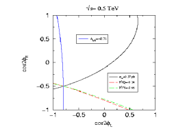
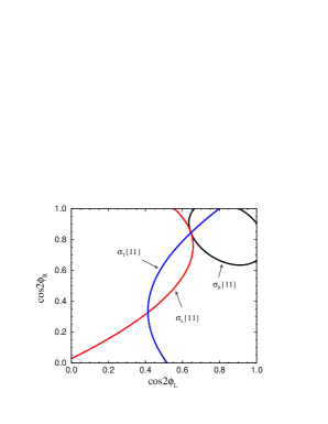
Figure 1: Use of initial or final state polarisation in the determination of $\cos 2\phi_{L}$ and $\cos 2\phi_{R}$.[1]

The knowledge of $m_{\chi_{1}^{\pm}}$ along with $\cos 2\phi_{L},\cos 2\phi_{R}$ then allows one to determine the parameters $M_{2}$, $\mu$ and $tan\beta$ upto a two fold ambiguity. Instead of using the polarisation information of the produced charginos, if polarised beams are available, measurement of $\sigma_{L}^{11},\sigma_{R}^{11}$ (where the superscripts 1,1 stand for the $\mbox{$\tilde{\chi}$}_{1}^{+}\mbox{$\tilde{\chi}$}_{1}^{-}$ production), allows determination of the mixing angles $cos2\phi_{L},cos2\phi_{R}$ upto a four fold ambiguity, assuming that one has the knowledge of $m_{\mbox{$\tilde{\chi}$}_{1}^{+}}$, $m_{\tilde{\nu}}$ from kinematics, and further assuming $g_{\tilde{\nu}\tilde{W}l}=g_{2}$. Use of cross-sections $\sigma_{T}^{11}$ with transeverse polarisation helps remove this ambiguity as shown in the right panel of Fig. 1. If production of all the charginos is allowed kinematically, unambiguous reconstruction of $\mu,M_{2}$ and tan$\beta$ is possible even without resorting to the use of transverse polarisation or the complicated study of the polarisation of the produced charginos. One can even test the relation $g_{e\tilde{\nu}\widetilde{W}}=g_{e\nu W}$. The results of an analysis, including only statistical errors, for $\int{\cal L}dt=1ab^{-1}$ are shown in Table 1. The left (right) column shows the input (extracted) values for the two chargino masses and $\cos 2\phi_{L},\cos 2\phi_{R}$.

Table 1: Comparison of the input and output values of the mixing angles in the chargino sector extracted from different chargino measurements for $\int{\cal L}dt=1{\rm ab}^{-1}$.

Input	Extracted
$m_{\mbox{$\tilde{\chi}$}_{1}^{\pm}}$ = 128 GeV,	$m_{\mbox{$\tilde{\chi}$}_{1}^{\pm}}$ = 128 $\pm 0.04$GeV,
$m_{\mbox{$\tilde{\chi}$}_{2}^{\pm}}$ = 346 GeV.	$m_{\mbox{$\tilde{\chi}$}_{2}^{\pm}}=346$ $\pm 0.25$ GeV.
$\cos 2\phi_{L}=0.645$,	$\cos 2\phi_{L}=0.645\pm 0.02,$
$\cos 2\phi_{R}=0.844.$	$\cos 2\phi_{R}=0.844\pm 0.005$.
$g_{e\tilde{\nu}\tilde{W}}/g_{e\nu W}=1$	$g_{e\tilde{\nu}\tilde{W}}/g_{e\nu W}=1\pm 0.01$

Using these uniquely determined values of $\cos 2\phi_{L},\cos 2\phi_{R}$ and the chargino masses, one can then extract $M_{2}$, $\mu$ and tan$\beta$ uniquely.

Table 2: The input and output values of $M_{2},\mu$ and $\tan\beta$ for two input points for an integrated luminosity $1ab^{-1}$.

parameter	Input	Extracted	Input	Extracted
$M_{2}$	152	$152\pm 1.75$	150	$150\pm 1.2$
$\mu$	316	$316\pm 0.87$	263	$263\pm 0.7$
$tan\beta$	3	3 $\pm$ 0.69	30	$>$ 20.2

Table 2 shows again the input and extracted values of $M_{2},\mu,\tan\beta$ for two different inputs. We see that the determination can be quite precise, except in the situation with large tan$\beta$. This is easy to understand as all the chargino variables are proportional to $\cos 2\beta$. Recall, however, that the $1\sigma$ errors shown here are purely statistical. An analysis including full detector effects, using this beautiful method which does not even require beam polarisation, might indeed be worthwhile in view of its promise.

2.2 Determination of $m_{\mbox{$\tilde{\chi}$}_{1}^{+}}$ through its $\tilde{\tau_{1}}$ decay.[2]

These authors looked at the determination of the chargino mass $m_{\mbox{$\tilde{\chi}$}_{1}^{\pm}}$, in the large tan $\beta$ (tan $\beta>$ 40) case where one expects a light stau $\tilde{\tau_{1}}$. If a mass heirarchy (expected at large $tan\beta$ in (M)SUGRA scenario as well) : $m(\tilde{l})>m(\mbox{$\tilde{\chi}$}_{1}^{+})>m(\tilde{\tau_{1}})>m(\mbox{$\tilde{\chi}$}_{1}^{0})$ exists, then $\mbox{$\tilde{\chi}$}_{1}^{+}$ decays into a $\tilde{\tau_{1}}\nu_{\tau}$ almost 100 % of the time. Thus the process used to study $\mbox{$\tilde{\chi}$}_{1}^{+}\mbox{$\tilde{\chi}$}_{1}^{-}$ production will now be $\mbox{$e^{+}e^{-}$}\to\mbox{$\tilde{\chi}$}_{1}^{+}+\mbox{$\tilde{\chi}$}_{1}^{-}\to$ ${\tilde{\tau}}_{1}^{+}\nu_{\tau}{\tilde{\tau}}_{1}^{-}\bar{\nu_{\tau}}\to$ $\tau^{+}\tau^{-}\mbox{$\tilde{\chi}$}_{1}^{0}\mbox{$\tilde{\chi}$}_{1}^{0}\nu_{\tau}\bar{\nu_{\tau}}$. For the mass heirarchy given above, we can assume $m_{{\tilde{\tau}}_{1}},m_{\mbox{$\tilde{\chi}$}_{1}^{0}}$ to be known from studies of ${\tilde{\tau}}_{1}^{+}{\tilde{\tau}}_{1}^{-}$ production. The main backgrounds are $2\gamma$, WW and ZZ. Using the $E_{jet}$ distribution ($\tau$ is detected as a thin jet) for $\int{\cal L}dt=200fb^{-1}$, with an input $m_{\mbox{$\tilde{\chi}$}_{1}^{+}}$ = 172 GeV, $m_{\tilde{\tau_{1}}}$ = 152 GeV and $m_{\mbox{$\tilde{\chi}$}_{1}^{0}}$ = 87 GeV, the authors find $m_{\mbox{$\tilde{\chi}$}_{1}^{+}}=171.3\pm 0.5$ GeV. The corresponding $\Delta\chi^{2}$ is shown in

Figure 2: $\Delta\chi^{2}$ as a function of $m_{\mbox{$\tilde{\chi}$}_{1}^{+}}$ for an integrated luminosity of 200 fb^-1.

Fig. 2.

2.3 Effects of radiative corrections on kinematic reconstruction of squark mass.[3]

The authors studied here $\mbox{$e^{+}e^{-}$}\ \to\tilde{q}{\tilde{q}}^{*}$. They included the radiative corrections to production and decay as well as the effects of the ISR. They used two estimators for the mass of $\tilde{q}$ : 1) $m_{\tilde{q},min}$[16] for two body final states and 2) $E_{jet}$ distribution. For an integrated luminosity of $50fb^{-1}$ and an input value of $m_{\tilde{q}}$ = 300 GeV, the authors found $m_{\tilde{q}}$ = 297.7 $\pm$ 2 GeV and $m_{\tilde{q}}$ = 303 $\pm$ 2.9 GeV from the two estimators $m_{\tilde{q},min}$ and $E_{jet}$ distributions respectively. The results are shown in Fig. 3.

Figure 3: $\chi^{2}$ as a function of $m_{\tilde{q}}$ for an integrated luminosity of 50 fb^-1.[3]

Thus it is seen that the effect of higher order corrections to decays does not deteriorate the utility of the estimator $m_{\tilde{q},min}$. The effect of hadronisation is not yet included in this analysis.

2.4 $\mbox{$e^{+}e^{-}$}\to\tilde{t_{1}}\tilde{t_{1}^{*}}h$ with explicit CP violation.[4]

The author here has looked at explicit CP violation in the MSSM higgs sector and loop effects (essentially the effects of large third generation trilinear term) on the Higgs potential with complex $A_{t}$. Essentially changes in $m_{{\tilde{t}}_{1}},g_{{\tilde{t}}_{1}{\tilde{t}}_{1}^{*}h}$ due to loop effects were calculated. There are two CP violating phases Arg($\mu$) and Arg($A_{t}$). The author chooses to satisfy the electric dipole constraints as well as cosmological ones[17] : i) Arg($\mu)<10^{-2}$ ii) $m_{\tilde{g}}>400$ GeV (iii) $|A_{e}|,|A_{u,c}|,|A_{d,e}|<10^{-3}|\mu|$ and iv) maximal mixing in the stop sector $|A_{t}|=|\mu cot\beta|$.

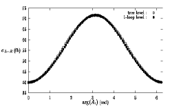
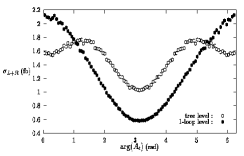
Figure 4: Effect of loop corrections on $\sigma(\tilde{t_{1}}\tilde{t_{1}}^{*})$ (left) and $\sigma(\tilde{t_{1}}\tilde{t_{1}}^{*}h)$ (right) as a function of $Arg(A_{t})$ ($\sqrt{s}=500$ GeV, $\mu=500$ GeV, $|A_{t}|=250$ GeV, $M_{A}\simeq 194$ GeV, $\tan\beta=2$, and $M_{\rm SUSY}=500$ GeV).

Fig. 4 shows $\sigma_{L+R}(\mbox{$e^{+}e^{-}$}\to{\tilde{t}}_{1}{\tilde{t}}_{1}^{*})$ and $\sigma_{L+R}(\mbox{$e^{+}e^{-}$}\to{\tilde{t}}_{1}{\tilde{t}}_{1}^{*}h)$ in the left and the right panels respectively. We see that though the loop effects are minimal in ${\tilde{t}}_{1}{\tilde{t}}_{1}^{*}$ production, the dependence on arg($A_{t}$) is quite strong; on the other hand for $\mbox{$e^{+}e^{-}$}\to{\tilde{t}}_{1}{\tilde{t}}_{1}^{*}h$ the cross sections are quite small but loop effects are substantial and can be as much as 100 %. The figure shows this for values of parameters given in the figure caption. The interesting cross-sections are $\sim$ few fb. A possible discussion of extracting $|A_{t}|,Arg(A_{t})$ by combining the measurements of these cross-sections with the knowledge of higgs masses has been sketched and seems worth pursuing.

2.5 Chargino/neutralino production and cascade decays of LSP through ${R\!\!\!/}_{p}$ couplings at $e^{+}e^{-}$ colliders.[5]

In this work the authors consider $\mbox{$e^{+}e^{-}$}\to\mbox{$\tilde{\chi}$}_{i}^{+}\mbox{$\tilde{\chi}$}_{j}^{-}$ and $\mbox{$e^{+}e^{-}$}\to\mbox{$\tilde{\chi}$}_{i}^{0}\mbox{$\tilde{\chi}$}_{j}^{0}$. Once the LEP constraints on $m_{\mbox{$\tilde{\chi}$}_{1}^{\pm}}$ are imposed, it is found that over a large part of the region of parameter space which allows $\mbox{$\tilde{\chi}$}_{1}^{+}$ within the reach of a 500 GeV linear collider, $\mbox{$\tilde{\chi}$}_{3}^{0},\mbox{$\tilde{\chi}$}_{4}^{0}$ and $\mbox{$\tilde{\chi}$}_{2}^{+}$ are almost always beyond its reach, at least in the framework of the (C)MSSM. Hence it is sufficient to consider i) $\mbox{$e^{+}e^{-}$}\to\mbox{$\tilde{\chi}$}_{1}^{0}\mbox{$\tilde{\chi}$}_{2}^{0}$ , ii)$\mbox{$e^{+}e^{-}$}\to\mbox{$\tilde{\chi}$}_{2}^{0}\mbox{$\tilde{\chi}$}_{2}^{0}$ and iii) $\mbox{$e^{+}e^{-}$}\to\mbox{$\tilde{\chi}$}_{1}^{+}\mbox{$\tilde{\chi}$}_{1}^{-}$. Further, using the approximate degeneracy of $\mbox{$\tilde{\chi}$}_{1}^{\pm}$ and $\mbox{$\tilde{\chi}$}_{2}^{0}$, the number of decay chains to be considered are reduced to managable numbers. The authors work in the weak coupling limit of ${R\!\!\!/}_{p}$ and consider the effect of ${R\!\!\!/}_{p}$ only for the LSP decay. For the ${L\!\!\!/}$ $\lambda$ couplings the final state will consist of m leptons and ${E\!\!\!/}_{T}$; for the ${L\!\!\!/}$ and ${B\!\!\!/}$ $\lambda^{{}^{\prime}}$ couplings it will consist of m leptons, n jets and ${E\!\!\!/}_{T}$ whereas ${B\!\!\!/}$ $\lambda^{"}$ couplings give rise to final state with only jets. The authors considered different sources of background in each case, chose different points in the parameter space to consider the chargino/neutralinos states with different gaugino/higgsino content and studied the process in a parton level Monte Carlo, with appropriate cuts on leptons and jets to reduce/remove background.

Table 3: Showing the contributions (in fb) of different (light) chargino and neutralino production modes to multi-lepton signals at the NLC in the case of $\lambda$ couplings. The last column shows the SM background.

	Signal	$\widetilde{\chi}^{0}_{1}\widetilde{\chi}^{0}_{1}$	$\widetilde{\chi}^{0}_{1}\widetilde{\chi}^{0}_{2}$	$\widetilde{\chi}^{0}_{2}\widetilde{\chi}^{0}_{2}$	$\widetilde{\chi}^{+}_{1}\widetilde{\chi}^{-}_{1}$	Signal	Bkgd.
						fb	fb
A	$1\ell+E_{T}/\;\>$	$1.1$	$0.4$	$0.2$	$1.5$	$3.2$	$8272.5$
	$2\ell+E_{T}/\;\>$	$14.9$	$5.2$	$1.8$	$15.3$	$37.2$	$2347.4$
	$3\ell+E_{T}/\;\>$	91.7	25.3	7.2	71.6	195.8	1.5
	$4\ell+E_{T}/\;\>$	212.8	49.6	13.6	152.8	428.8	0.4
	$5\ell+E_{T}/\;\>$	0.0	37.8	19.3	113.5	170.6	-
	$6\ell+E_{T}/\;\>$	0.0	39.6	21.6	26.9	88.0	-
	$7\ell+E_{T}/\;\>$	0.0	0.0	11.9	0.0	11.9	-
	$8\ell+E_{T}/\;\>$	0.0	0.0	8.0	0.0	8.0	-

Table 3 shows for a particular point results of the Monte Carlo analysis for the case of $\lambda$ couplings. In case of these signals, particularly for the case of $\lambda^{"}$ couplings the final state involves a large number of partons with/out leptons. Some of these partons may merge together in jet definitions, removing the connection between the jet multiplicity and the number of initial partons in the final state. It is pointed out that kinematic mass reconstructions can be used to study the multijet events and identify those coming from ${B\!\!\!/}$ couplings. Fig. 5 shows the distribution in invariant mass constructed from the hardest jet and all the other jets in the same hemisphere, and the same for the hardest jet in the opposite hemisphere.

Figure 5: Illustrating the distribution in invariant mass reconstructed from ($a$) the hardest jet and all jets in the same hemisphere, and ($b$) the hardest jet in the opposite hemisphere and all remaining hadronic jets, when all contributions are summed over (signal only), for a chosen point in the parameter space.[5]

The distribution shows clear peaking at $m_{\mbox{$\tilde{\chi}$}_{1}^{0}}$ as well as a sharp cutoff at $m_{\mbox{$\tilde{\chi}$}_{1}^{\pm}}\approx m_{\mbox{$\tilde{\chi}$}_{2}^{0}}$. Thus kinematic distributions can be used quite effectively even for the case of the multijet events. Effect of backgrounds on this distribution need to be studied, however.

2.6 Wino LSP in AMSB at $e^{+}e^{-}$ colliders.[6]

In the AMSB scenario, $\mbox{$\tilde{\chi}$}_{1}^{0},\mbox{$\tilde{\chi}$}_{1}^{+}$ are both almost pure Winos and almost degenerate. The authors investigate here $\mbox{$e^{+}e^{-}$}\to\tilde{e}(\to e\mbox{$\tilde{\chi}$}_{1}^{0})+\tilde{e^{*}}(\to\nu\mbox{$\tilde{\chi}$}_{1}^{+})\longrightarrow e\mbox{$\tilde{\chi}$}_{1}^{0}\nu\mbox{$\tilde{\chi}$}_{1}^{+}(\to\mbox{$\tilde{\chi}$}_{1}^{0}+\pi)\longrightarrow e\mbox{$\tilde{\chi}$}_{1}^{0}\nu\mbox{$\tilde{\chi}$}_{1}^{0}\pi$. The B.R. for $\mbox{$\tilde{\chi}$}_{1}^{+}\to\mbox{$\tilde{\chi}$}_{1}^{0}+\pi$ is $\sim 96-98\%$. The authors look at the regions in $M_{3/2}-m_{0}$ plane ($m_{0}$ being the scalar mass added to make the slepton masses nontachyonic) for a range of $tan\beta$ values. They found that large regions, allowed by all the currrent constraints, have large cross-sections $\sim 10-100$ fb at $\sqrt{s}$ = 1000 GeV, after kinematical cuts on the $e^{-}$ and B.R. are included, as shown in Fig. 6.

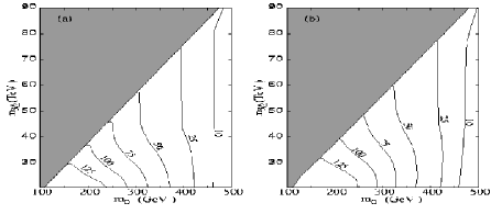
Figure 6: Regions in the $M_{3/2}-m_{0}$ plane along with contours of constant cross-section expected for the signal in the AMSB scenario. The shaded regions are ruled out by various constraints.[6]

The signal is a fast e($\mu)+\mbox{${E\!\!\!/}_{T}$}$ and a soft $\pi$. The soft $\pi$ can give rise to a displaced vertex with impact parameter resolved if c$\tau<$ 3cm. If $\mbox{$\tilde{\chi}$}_{1}^{+}$ decay length is long (c$\tau>$ 3cm), then one sees a heavily ionising track. The authors looked at the cross-section after cuts and find that with 50 (500) $fb^{-1}$ integrated luminosity one expects $\sim 10^{3}(10^{4})$ events at $\sqrt{s}$ = 500 (1000) GeV. It is also to be noted that this case is different from the almost degenerate $\mbox{$\tilde{\chi}$}_{1}^{+},\mbox{$\tilde{\chi}$}_{1}^{0}$ scenario in the MSSM where the chargino/neutralino are higgsinos.[18]

2.7 Squark, slepton production at $\gamma\gamma$ colliders and decays through ${R\!\!\!/}_{p}$ interactions.[8]

The authors performed a study of $\mbox{$\gamma\gamma$}\to\tilde{f}{\tilde{}}f^{*}$, followed by the $R_{p}$ conserving decays $\tilde{f}\to f+\mbox{$\tilde{\chi}$}_{1}^{0},\tilde{f}\to f^{\prime}+\mbox{$\tilde{\chi}$}_{1}^{+}$ along with the ${R\!\!\!/}_{p}$ decays $\tilde{f}\to f_{1}f_{2}$ where $f_{1},f_{2}$ are SM fermions ($q_{1}q_{2}$ for $\tilde{l}$, lq for $\tilde{q}$). One of the features worth nothing is that the production cross-section of scalars can be enhanced by an appropriate choice of polarisation.[19] This can be seen in Fig. 7 where $\sigma(\mbox{$\gamma\gamma$}\to{\tilde{l}}^{+}{\tilde{l}}^{-})$ has been plotted for different polarisation combinations for $\sqrt{s_{\mbox{$e^{+}e^{-}$}}}$ = 1 TeV, using the back-scattered laser spectrum. They have then calculated the branching ratios for the $R_{p}$ conserving as well as ${R\!\!\!/}_{p}$ two body decays. These of course depend on the SUSY model parameters $M_{2},\mu$. The signal for ${R\!\!\!/}_{p}$ decays is simply 4f final states. The authors use kinematic cuts to reduce the background, e.g. from heavy flavours. Further, they reconstruct lj, $j_{1}j_{2}$ invariant masses and demand that $|M_{lj}^{(1)}-M_{lj}^{(2)}|$ $<$ 10 GeV for the squark signal and $|M_{ij}-M_{kl}|$ $<$ 10 GeV for the slepton signal. The combinatorial background is quite high for the second case. The panel on the right in Fig. 7 shows the reach in $M_{2}-m_{\hat{l}}$ plane for $\lambda^{\prime}$ coupling = 0.02. The dependence on $M_{2}$ comes from the dependence of the ${R\!\!\!/}_{p}$ B.R. on $M_{2}$.

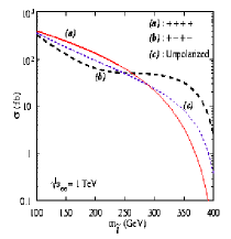
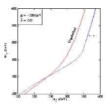
Figure 7: Production cross-section of sfermions as a function of $m_{\tilde{f}}$(left panel), reach in $M_{2},m_{\tilde{f}}$ plane with polarised and unpolarised option(right panel).[8] All the parameters are as shown in the figure.

3 Probing extra dimensions at $\mbox{$e^{+}e^{-}$}/\mbox{$\gamma\gamma$}/e\gamma/\mbox{$e^{-}e^{-}$}$ colliders.

3.1 Looking for the radion in RS model at $e^{+}e^{-}$ colliders.[11]

These authors have looked at the phenomenology of the radion field $\phi$ which stabilizes the RS scenario.[20] This field can be lighter than the KK excitations and its couplings to the SM particles are determined by general co-variance in four dimensional space-time. There are two parameters: $m_{\phi}$ and a scale $\Lambda_{\phi}\sim 0(v)$ where $v$ is the vacuum expectation value of the Higgs field. The authors have computed two body decay modes of $\phi$ whose couplings to fermions are $\sim g^{SM}_{hf\bar{f}}{v}{\Lambda\phi}$. Regions for low $\Lambda_{\phi}-m_{\phi}$ are ruled out by L3 bound on $m_{h}$ and the requirement of perturbative unitarity[21] of the couplings of $\phi$. Cross-sections for production of $\phi$ at $e^{+}e^{-}$ colliders have been computed and the region in $m_{\phi}-\Lambda_{\phi}$ plane that can be probed has been identified. This is shown in Fig. 8 as contours of constant cross-section in the plane.

Figure 8: Regions in the $\Lambda_{\phi}$ - $m_{\phi}$ plane along with contours of constant cross-sections for the production of $\phi$.[11]

3.2 Indirect effects of large extra dimensions.[12, 13, 14, 15]

These authors have looked at essentially the ADD model[22] and studied the indirect effects on $t\bar{t}$, dijet production at $\gamma\gamma$ colliders and graviton production in $e\gamma$ collisions. They have also studied the indirect effects of the gravitons in the $e^{-}e^{-}$ collisions in the RS model.[20] In the study of dijet/$t\bar{t}$ production[12, 13], the authors have used the idealized backscattered laser spectrum and the total integrated luminosity of 100 $fb^{-1}$. They observe that the reach of these colliders for the scale $M_{s}$ can be increased substantially by an effective use of polarisation. They have obtained the possible bounds by looking only at the total $t\bar{t}$ cross-sections.

Table 4: Limits on the scale $M_{s}$ that can be reached[13] in top production at $\gamma\gamma$ colliders for polarised leptons and lasers in case of ADD model.[22]

$(\lambda_{e1}\lambda_{e2}\lambda_{l1}\lambda_{l2})$	$\sqrt{s}$ GeV	$M_{s}$ (TeV)
	500	1.95
(+ - - -)	1000	4.6
	1500	6.0
	500	2.5
(+ - - +)	1000	4.8
	1500	6.4

Table 4 shows their results. These bounds have been obtained by using only the statistical errors. The analysis can be improved by using distributions in kinematic variables as well as by considering the systematic errors. In dijet production, e.g. the ‘resolved’ photon contribution[23] could be nontrivial, which has not been considered in the analysis.

Direct study of graviton production in $e\gamma\to eG^{(n)}$ can also be used to probe the ‘large’ extra dimensions.[14] The signature of such graviton production will be an isolated $e^{-}$ and missing energy. The backgrounds are $e\gamma\to eZ\to e\nu\bar{\nu}$ and $e\gamma\to\nu w\to\nu\nu e$. These backgrounds had been evaluated in a study of $e\gamma\to\tilde{e}\mbox{$\tilde{\chi}$}_{1}^{0}\to e+\mbox{$\tilde{\chi}$}_{1}^{0}+\mbox{$\tilde{\chi}$}_{1}^{0}$.[9] Using idealized backscattered laser spectrum, L = $\int{\cal L}dt=100\>fb^{-1}$, demanding $\sigma\sqrt{L}/\sqrt{B}>5$ and putting cuts on $P_{T}^{l},|Y_{e}|$ to remove the background, the reach for $M_{s}$ in the ADD model[22] is between 4-2 TeV for n=2 to 6. The use of $e^{-}$ polarization to reduce eW background is absolutely essential. Using polarized lasers might improve the reach even further, but it has not been studied yet.

Indirect effects in $e^{-}e^{-}$ collisions in the RS model also provide a good reach for the graviton mass $M_{1}$. The analysis looks at $\mbox{$e^{-}e^{-}$}\to\mbox{$e^{-}e^{-}$}$ and puts cuts of $\theta_{e}>10^{0},P_{T}^{l}>10$ GeV for the detected electrons. They state their results in terms of $c_{0}=\frac{1}{8\pi}\frac{{\cal K}}{\overline{M_{p}}}$ where $\overline{M_{p}}$ is the reduced Planck mass and ${\cal K}$ is the extra mass scale in the model.[20]

Table 5: Limits on mass $M_{1}$ of the first graviton excitation in the RS model[20] at an $e\gamma$ collider for different beam energies, luminosities and model parameter $c_{0}({\cal K})$.

$\sqrt{s}$	$\int Ldt$ ( fb -1)	$c_{0}$	$M_{1}$ (TeV)
500	500	0.01	1.3
	500	0.1	4
1000	500	0.01	2.4
	100	0.1	6.4

Table 5 gives the reach[15] for mass $M_{1}$ of the first graviton excitation for different beam energies, luminosities and values of model parameter $c_{0}({\cal K})$. Here use of polarisation improves the reach. This analysis has used the information on the distribution of $e^{-}$ and assumed a modest polarisation of 80%. The estimates of error, however, are only statistical ones.

References

- [1] S.Y. Choi, A. Djouadi, H. Dreiner, J. Kalinowski and P.M. Zerwas, Eur. Phys. J. C7, 123 (1999) ; S.Y. Choi, A. Djoudai, H.S. Song and P.M. Zerwas, Eur. Phys. J. C8, 669 (1999) ; S.Y. Choi, A. Djouadi, M. Guchait, J. Kalinowski, H.S. Song and P.M. Zerwas, Eur. Phys. J. C14, 535 (2000).
- [2] Y. Kato, hep-ph/9910293.
- [3] M. Drees, Oscar J.P. Eboli, R. M. Godbole and S. Kraml, in the SUSY Working Group for the workshop ‘Physics at the TeV colliders’ Les Houches, June 1999, hep-ph/0005142.
- [4] S. Bae, Phys. Lett. B 489, 171 (2000).
- [5] D. Ghosh, R.M. Godbole and S. Raychaudhuri, hep-ph/9904233
- [6] D. Ghosh, P. Roy and S. Roy, Journal of High Energy Physics 8, 031 (2000).
- [7] S.Y. Choi, H.S. Song and W.Y. Song, Phys. Rev. D 61, 075004 (2000).
- [8] D. Choudhury and A. Datta, hep-ph/0005082.
- [9] D. Ghosh and S. Raychaudhuri, Phys. Lett. B 422, 187 (1998), hep-ph/9711473.
- [10] D. Ghosh and S. Roy, hep-ph/0003225.
- [11] S. Bae, P. Ko, H.S. Lee and Jungil Lee, Phys. Lett. B 487, 299 (2000)
- [12] D. Ghosh, P. Mathews, P. Poulose and K. Sridhar, Journal of High Energy Physics 4, 9911 (1999), hep-ph/9909567.
- [13] P. Mathews, P. Poulose and K. Sridhar, Phys. Lett. B 461, 196 (1999), hep-ph/9905395.
- [14] D. Ghosh, P. Poulose and K. Sridhar, Mod.Phys.Lett. A15, 475 (2000), hep-ph/9909377.
- [15] D. Ghosh and S. Raychaudhuri, hep-ph/0007354.
- [16] J.L. Feng and D.E. Finnell, Phys. Rev. D 49, 2369 (1994).
- [17] A. Pilaftsis and C.E.M. Wagner, Nucl. Phys. B 553, 3 (1999); D. Chang, W.-Y. Keung and A. Pilaftsis, Phys. Rev. Lett. 82, 900 (1999).
- [18] C.M. Chen, M.Drees and J.F. Gunion, Phys. Rev. D 55, 330 (1997),Erratum:hep-ph/9902309.
- [19] S. Chakrabarti, D. Choudhury, R.M. Godbole and B. Mukhopadhyaya, Phys. Lett. B 434, 347 (1998), hep-ph/9804297.
- [20] L. Randall and R. Sundrum, Phys. Rev. Lett. 83, 3370 (1999); L. Randall and R. Sundrum, Phys. Rev. Lett. 83, 4690 (1999).
- [21] U. Mahanta and S. Rakshit, Phys. Lett. B 480, 176 (2000), hep-ph/0002049.
- [22] N. Arkani-Hamed, S. Dimopoulos and G. Dvali, Phys. Lett. B 429, 263 (1998).
- [23] M. Drees and R.M. Godbole,Z. Phys. C 59, 591 (1993), hep-ph/9203219.