Equilibrium and non-equilibrium properties associated with the chiral phase transition at finite density in the Gross-Neveu Model

Abstract

We study the dynamics of the chiral phase transition at finite density in the Gross-Neveu (GN) model in the leading order in large-$N$ approximation. The phase structure of the GN model in this approximation has the property that there is a tricritical point at a fixed temperature and chemical potential separating regions where the chiral transition is first order from that where it is second order. We consider evolutions starting in local thermal and chemical equilibrium in the massless unbroken phase for conditions pertaining to traversing a first or second order phase transition. We assume boost invariant kinematics and determine the evolution of the order parameter $\sigma$, the energy density and pressure as well as the effective temperature, chemical potential and interpolating number densities as a function of the proper time $\tau$. We find that before the phase transition, the system behaves as if it were an ideal fluid in local thermal equilibrium with equation of state $p=\epsilon$. After the phase transition, the system quickly reaches its true broken symmetry vacuum value for the fermion mass and for the energy density. The single particle distribution functions for Fermions and anti-Fermions go far out of equilibrium as soon as the plasma traverses the chiral phase transition. We have also determined the spatial dependence of the “pion” Green’s function $\langle\bar{\psi}(x)\gamma_{5}\psi(x)\bar{\psi}(0)\gamma_{5}\psi(0)\rangle$ as a function of the proper time.

I Introduction

The phase structure of QCD at non-zero temperature and baryon density is important for the physics of neutron stars and heavy ion collisions. The approximate phase structure for QCD with different numbers of quark flavors has been mapped out in various mean field and perturbative approximations ref:super1 ref:super2 ref:super3 ref:ref1 . The phase structure for two masless quark flavors (up and down) already reveals a rich sturcture. In addition to the well known chiral symmetry broken and restored phases, recent investigations have revealed the possibility of a color superconducting phase at low temperatures and relatively high densities. The transition to the superconducting phase as we increase $\mu$ at zero temperature is first order. On the other hand, in the chiral condensation regime at zero chemical potential, the phase transition as we increase the temperature to the unbroken mode is second order. This suggests that there is a regime at intermediate chemical potentials where the chiral phase transition is first order. Along the line separating the broken and unbroken chiral phases there is a tricritical point.

One of the most pressing experimental questions is to what extent experiments at the relativistic heavy ion collider RHIC can explore this rich phase structure and what would be the experimental consequences of having a quark-gluon plasma rather than a hadronic plasma following a collision of heavy ions. Since the production and evolution of the quark-gluon plasma in a heavy ion collision might be a nonequilibrium process, one needs to understand the evolution of an expanding, possibly out of equilibrium, plasma. We have considered a toy model, which has several properties in common with two flavor massless QCD to explore these nonequilibrium evolutions. The model we have found ref:us is a $1+1$ dimensional model of self interacting fermions, that has, in the leading order in large-N (LOLN) approximation a phase diagram with properties similar to that of massless two flavor QCD such as a tricritical point as well as a superconducting phase transition as one increases $\mu$ at low temperature. Since an ultrarelativistic collision leads to an essentially one dimensional expansion at early times, it is hoped that the rate of expansion in our toy model will be similar to that found in QCD so that the rate the system undergoes the phase transition will be similar to what would be found in a a more realistic $3+1$ dimensional expansion. Since this model has asymptotic freedom, the coupling constants run logarithmically in LOLN which is a feature shared with QCD. In this paper we will confine ourselves for studying the dynamics near the tricritical point in our toy model which for that case reduces to the Gross-Neveu model.

One of the questions important for RHIC is whether there are unambiguous experimental signatures resulting from a change in the nature of the phase transition as a function of the chemical potential (baryon density). In our toy model, the change is the difference from a first order to second order transition. In actuality this change might be the change from a first order transition to a crossover phenomena. Our approach is to directly determine the time evolution of the plasma starting from an initial point on the phase diagram above the chiral phase transition and watch the evolution through the phase transition. From the time evolving fermion mode functions one can calculate many physical quantities such as the current current correlation function which determines the dilepton rate as well as various particle correlation functions such as that for the pion. In this paper we determine single particle distributions functions as well as the composite particle pion correlation function to try to find the difference in experimentally measurable quantities when a plasma evolutions traversing say a first rather than a second order phase transition. For the purpose of studying the chiral phase transition, we can restrict ourselves to just a sector of our toy model in which it reduces to the well known Gross-Neveu (GN) model ref:GN . This simpler model allows us to study evolutions on both sides of a tricritical point. The exact phase structure of the Gross-Neveu model in dimensions $2\leq 4$ at finite temperature and chemical potential has been the subject of several recent investigations phase . Using both renormalization group methods, dimensional reduction methods as well as strong coupling expansions, it is thought that the line of chiral phase transitions in all these dimensions is either second order or weakly first order, which is the same situation as pertains in the leading order in large-N calculation. What is missing in the leading order large-N is real scatterings that could lead to rethermalization. Therefore, the findings of our simulations that the distributions of fermions and antifermions goes far out of equilibrium following the transition, might easily be modified by a more realistic simulation. The calculations presented here must be thought of as presenting the first field theory simulations at finite chemical potential of an evolution through a chiral phase transition with a realistic expansion rate for the plasma appropriate to a heavy ion collision. Future studies will remedy some of the shortcomings of this toy model, in that inhomogeneous plasmas will be studied as well as $1/N$ resummation methods will be used in future simulations which will still be based, however on Gross-Neveu like models albeit in $3+1$ dimensions as well as in $1+1$ dimensions. The approach we take here is to directly solve the evolution equations of a quantum plasma in leading order in large-N. A complementary approach is to study critical slowing near the critical point using ideas from universality and dynamical critical phenomena crit . Our interest is more in having a complete space time picture of an evolving quark plasma and our hope is that once we resum the LOLN approximation using Dyson equations and consider the $3+1$ dimensional version of this model that we will be able to address issues of critical slowing down. The calculations presented here in the toy model already exhibit the effects of how having small rather than zero quark masses at high temperatures change the time period of the transition. They also demonstrate how one can calculate all spatial correlation functions as well as the time evolution of the Temperature and chemical potential, and how a hydrodynamic approach can be quite accurate before the phase transiton.

Following a relativistic heavy ion collision, the ensuing plasma expands and cools traversing the chiral phase transition. In hydrodynamic simulations of these collisions Landau ; CFS ; Bjorken ; PRD , as well as in parton cascade models and other event genarator approaches Feynman ; BjCC ; CKS ; Lund ; Low ; Nussinov , one finds that it is a reasonable approximation to treat the initial phase of the expansion as a 1+1 dimensional boost invariant expansion along the beam ($z$) axis. In this approximation, the fluid velocity scales as $z/t$. In terms of the variables fluid rapidity $\eta={1\over 2}~{}{\rm ln}~{}\left({t+z\over t-z}\right)$ and fluid proper time $\tau=(t^{2}-z^{2})^{1/2}$, physical quantities such as $\sigma,\epsilon$ become independent of $\eta$, as discussed in refs. CFS ; Bjorken ; PRD . Such an approach was used in our field theory calculations of the production and evolution of disoriented chiral condensates in the O(4) $\sigma$ model in ref.ref:DCC . This approximation is valid for particles produced in the central rapidity region. To study more peripheral collisions a full inhomogenous calculation must be performed. This latter study has just started and will be the subject of a future paper.

These kinematical considerations translate into the expansion being homogeneous in the fluid rapdity $\eta$, which allows us to convert what would be a set of partial differential equations for the mode functions to a much simpler set of ordinary differential equations in the parameter $\tau$. The LOLN approximation we will use in obtaining the field equations has been been discussed earlier by ourselves and others in PRD ; CM ; PRL ; PRD2 ; covariant ; blsnoneq ; cmupittparnoneq ; ucsbnoneq and applied to the problem of disoriented chiral condensates in ref:DCC ; dccbdh . Extending the boost invariant simulation to $3+1$ dimensions so that transverse distributions can be studies is relatively simple.

In solving the time evolution equations for the quantum fields, the initial conditions for the fields are specified at $\tau=\tau_{0}$, that is, on a hyperbola of constant proper time. The $\tau$ evolving energy density and pressure are obtained from the expectation value of the energy momentum tensor. To discuss the production of particles we introduce the concept of an adiabatic number operator which is an adiabatic invariant of the LOLN Hamiltonian. Although our equations will be valid for arbitrary initial conditions, to study the regime around the tricritical point we will assume that at some initial proper time the system can be described by a Fermi-Dirac Distribution with given $\mu_{0}$ and $T_{0}$ in the comoving frame. In our simulations we will also choose the initial conditions on our mode functions to agree with the lowest order WKB approximation result. By choosing this initial condition on the mode functions, the adiabatic number operator then gives a smooth interpolation between the initial Fermi-Dirac distribrutions described by $\mu_{0}$, $T_{0}$ and the final outstate number operators. The rest of the paper is organized as follows. In section II we review the equlibrium properties of the GN model at finite $\mu$ and $T$ in the LOLN approximation. Particular attention is paid to the phase diagram. In section III we derive the action in curved coordinates in order to discuss the evolution in terms of the parameters $\tau$ and $\eta$. Section IV is concerned with renormalization and obtaining explicitly finite evolution equations. In section V we discuss our choice of initial conditions. In section VI we derive an expression for the expectation value of the energy momentum tensor and obtain expressions for the renormalized energy density and pressure in terms of the mode functions of the fermion field. In section VII we introduce the adiabatic number operator and obtain simple expressions for both the fermion and antifermion interpolating number operators in terms of the modes. In section VIII we discuss our numerical results for the proper time evolution of the effective fermion mass, $\mu$, $T$ as well as the interpolating number densities. In section IX we determine the time evolution of the pion correlation function. Some of the results we obtain in this article were summarized and presented at a Riken workshop usletter .

II Effective Potential and Phase Structure

The Lagrangian for the Gross-Neveu Model ref:GN is

$${\cal L}=-i\bar{\Psi}_{i}\gamma^{\mu}\partial_{\mu}\Psi_{i}-{1\over 2}g^{2}\left(\bar{\Psi}_{i}\Psi^{i}\right)^{2},$$ (1)

which is invariant under the discrete chiral group: $\Psi_{i}\rightarrow\gamma_{5}\Psi_{i}$. In leading order in large $N$ the effective action is

$$S_{eff}=\int d^{2}x\left[-i\bar{\Psi}_{i}\left(\not\partial+\sigma\right)\Psi^{i}-\frac{\sigma^{2}}{2g^{2}}\right]+{\rm tr}{\rm ln}S^{-1}[\sigma]~{},$$ (2)

where $S^{-1}(x,y)[\sigma]=\left(\gamma^{\mu}\partial_{\mu}+\sigma\right)\delta(x-y)$.

The phase structure of the GN model at finite temperature and chemical potential in this approximation has been known for a long time ref:us ref:GN2 and is displayed in Fig. 1.

Figure 1: Phase Structure at finite Temperature and Chemical Potential $\mu$. Dotted lines correspond to approximate analytic results described in the text.

This figure summarizes several facts. In the GN model there is spontaneous symmetry breaking of the discrete chiral symmetry at zero chemical potential and temperature. The value of the vacuum expectation value of $\sigma$ at the minimum of the effective potential determines and is equal to the mass of the fermion $m_{f}$ in this approximation. At zero temperature, the symmetry is restored at a critical value of the chemical potential $\mu_{c}={m_{f}\over\sqrt{2}}$. This phase transition is first order. At zero chemical potential the system undergoes a second order phase transition to the unbroken symmetry phase as the temperature is increased. As a result of these two facts, at some point in the phase diagram there is a tricritical point which can be determined numerically to be at ${\mu_{c}\over m_{f}}=.608,{T_{c}\over m_{f}}=.318$. These facts can be ascertained by studying the effective potential in LONL which is given by

$$V_{eff}(\sigma^{2},T,\mu) = {\sigma^{2}\over 4\pi}[\ln~{}{\sigma^{2}\over m_{f}^{2}}-1]$$ (3)

$$- {2\over\beta}\int_{0}^{\infty}{dk\over 2\pi}~{}[\ln~{}(1+e^{-\beta(E-\mu)})+\ln(1+e^{-\beta(E+\mu)})]~{}.$$

The integrals can be evaluated in the high temperature (and small ${\mu\over T}$) regime. Keeping the leading terms in the expansion one obtains

$$V_{eff}(\sigma^{2},T,\mu)={\sigma^{2}\over 4\pi}\biggl{(}\ln~{}{T^{2}\over T_{c}^{2}}+{7\over 2}{\zeta(3)\over\pi^{2}T^{2}}(\mu^{2}+{\sigma^{2}\over 4})\biggr{)}~{},$$ (4)

which leads to the relationship:

$$T_{c}={m_{f}\over\pi}\exp[\gamma-{7\mu^{2}\zeta(3)\over 4\pi^{2}T_{c}^{2}}]$$ (5)

for the phase transition temperature in the regime where the transition is second order and ${\mu\over T}<<1$. At small $\mu^{2}$ one has approximately

$$T_{c}={m_{f}\over\pi}e^{\gamma}[1-{7\mu^{2}\zeta(3)\over 4\gamma m_{f}^{2}e^{\gamma}}]~{}.$$ (6)

In the low temperature regime for the case $\sigma\leq\mu$ we can make an approximation to the Fermi-Dirac distribution function that again allows us to perform all the integrals analytically and determine an approximate analytic form for the Effective Potential. We write the derivative of the potential in the form:

$${\partial V\over\partial\sigma}={\sigma\over 2\pi}\ln{\sigma^{2}\over m_{f}^{2}}+{\sigma\over\pi}\int_{0}^{\infty}{dk\over E}[2-\tanh{E+\mu\over 2T}-\tanh{E-\mu\over 2T}]~{},$$ (7)

where $E=\sqrt{k^{2}+\sigma^{2}}$, and then replace the function $\tanh({E-\mu\over T})$ with the straight line interpolation:

$$\tanh(x)\rightarrow\{1~{}{\rm if}~{}x>2;~{}-1~{}{\rm if}~{}x<2{\rm and}~{}x~{}{\rm if}~{}|x|\leq 2\}~{}.$$ (8)

Using this approximation the integrals can be performed and $V$ determined. The results are shown as the dotted curve in Fig. 1. The analytic expression is given in ref:us .

When $T=0$, the effect of the chemical potential is the most dramatic. In that limit $\tanh(x)=\epsilon(x)$, and we obtain the exact result

$${\partial V\over\partial\sigma} ={\sigma\over 2\pi}\ln{\sigma^{2}\over m_{f}^{2}}+{\sigma\over\pi}\int_{0}^{\sqrt{\mu^{2}-\sigma^{2}}}{dk\over E}\Theta(\mu-\sigma)$$ (9)

$$={\sigma\over 2\pi}\ln{\sigma^{2}\over m_{f}^{2}}+{\sigma\over\pi}\Theta(\mu-\sigma)\{\ln(1+\sqrt{1-\sigma^{2}/\mu^{2}})-{1\over 2}\ln{\sigma^{2}\over\mu^{2}}\}~{}.$$

This can be integrated to give the result that for $\sigma\leq\mu$ the effective potential is given by:

$$V_{eff}={1\over 4\pi}\{\sigma^{2}(2~{}\ln[{\mu+\sqrt{\mu^{2}-\sigma^{2}}\over m_{f}}]-1)-2\mu\sqrt{\mu^{2}-\sigma^{2}}+C(\mu)\}~{},$$ (10)

wheras, for $\sigma>\mu$ the effective potential is equal to its $\mu=0$ value, namely

$$V_{eff}={\sigma^{2}\over 4\pi}[\ln~{}{\sigma^{2}\over m_{f}^{2}}-1]+C(\mu)~{}.$$ (11)

The integration constant can be fixed by choosing $V_{eff}(\sigma=0)=0,$ which yields

$$C(\mu)={\mu^{2}\over 2\pi}~{}.$$ (12)

At $T=0$ in the broken symmetry phase the effective mass is independent of $\mu$ and is given by $m_{f}$, its value when $\mu=0,T=0$. When $\mu^{2}>m_{f}^{2}/2$ then the true minimum is at $\sigma=0$. The transition at $\mu^{2}=m_{f}^{2}/2$ is a first order transition as can be determined by eq. (9) and eq.(10). In the toy model ref:us with two coupling constants, which also has a superconducting phase, the first order transition takes place at the point:

$$\mu^{2}={m_{f}^{2}\over 2}(1-e^{-4\pi\delta})~{},$$ (13)

where $\delta$ is the difference of the inverse of the two coupling constants of the model ref:us , namely $\delta={1\over\kappa}-{1\over 2\lambda}$. When the second coupling constant $\kappa\rightarrow 0^{+}$, the toy model reduces to the GN model.

In our straight line interpolation of the $\tanh$ function we obtain for the tricritical point which seperates the regime between the first and second order phase transitions: ${\mu_{c}\over m_{f}}=.661,~{}~{}~{}{T_{c}\over m_{f}}=.31$ as opposed to the exact result

$${\mu_{c}\over m_{f}}=.608,~{}~{}~{}~{}~{}~{}{T_{c}\over m_{f}}=.318.$$ (14)

In Fig. 1 we plot the exact numerical result for the phase diagram along with these two approximate results. In Figs. 2, 3 we show the evolution of the effective potentials for the first order and second order phase transitions when we keep $\mu$ fixed on two sides of the critical value and we decrease the temperature.

Figure 2: Evolution of $V_{eff}$ as a function of $T$. This is for a first order transition.

Figure 3: Evolution of $V_{eff}$ as a function of $T$. This is for a second order transition.

III Gross-Neveu model in curvilinear coordinates

In order to make best use of the kinematic constraint that we are in a scaling regime where the fluid velocity is $v=z/t$, we make a coordinate transformation to the light-cone variables $\tau$ and $\eta$, which are the fluid proper time and rapidity respectively. These coordinates are defined in terms of the ordinary lab-frame Minkowski time $t$ and coordinate along the beam direction $z$ by

$$z=\tau\sinh\eta\quad,\quad t=\tau\cosh\eta\,.$$ (15)

We shall use the metric convention $(-+)$ which is commonly used in the curved-space literature. In what follows, we use Greek indices for the curvilinear coordinates $\tau$ and $\eta$, and Latin indices for the Minkowski coordinates $z$ and $t$. To obtain the Fermion evolution equations in the new coordinate system it is simplest to use a coordinate covariant action such as that used in field theory in curved spaces, even though here the curvature is zero.

The Minkowski line element in these coordinates has the form

$${ds^{2}}={-d\tau^{2}+{\tau}^{2}{d\eta}^{2}}\,.$$ (16)

Hence the metric tensor is given by

$$g_{\mu\nu}={\rm diag}(-1,\tau^{2})~{}.$$ (17)

with its inverse determined from $g^{\mu\nu}g_{\nu\rho}=\delta^{\mu}_{\rho}$. This metric is a special case of the Kasner metric Birrell_Davies .

The vierbein $V^{a}_{\mu}$ transforms the curvilinear coordinates to Minkowski coordinates,

$$g_{\mu\nu}=V^{a}_{\mu}V^{b}_{\nu}\eta_{ab}\,,$$ (18)

where $\eta_{ab}={\rm diag}\{-1,1\}$ is the flat Minkowski metric. A convenient choice of the vierbein for the metric (17) for our problem is

$$V_{\mu}^{a}={\rm diag}\{1,\tau\}~{},$$ (19)

so that

$$V^{\mu}_{a}={\rm diag}\left\{1,{\frac{1}{\tau}}\right\}\,.$$ (20)

The determinant of the metric tensor is given by

$$\det V=\sqrt{-g}=\tau\,.$$ (21)

The action for the Gross-Neveu Model in general curvilinear coordinates (see Birrell_Davies ) with metric $g_{\mu\nu}$ is

$$S=\int d^{2}x\,({\rm{det}}\,V)\left[{\frac{-i}{2}}\bar{\Psi}_{i}\tilde{\gamma}^{\mu}\nabla_{\mu}\Psi^{i}+{\frac{i}{2}}(\nabla^{{\dagger}}_{\mu}\bar{\Psi}_{i})\tilde{\gamma}^{\mu}\Psi^{i}-i\sigma\bar{\Psi}_{i}\Psi^{i}-\frac{\sigma^{2}}{2g^{2}}\right]~{}.$$ (22)

The covariant derivative is (see Weinberg )

$$\nabla_{\mu}\Psi_{i}\equiv(\partial_{\mu}+\Gamma_{\mu})\Psi_{i}~{},$$ (23)

where the spin connection $\Gamma_{\mu}$ is given by

$$\Gamma_{\mu}=\frac{1}{2}\Sigma^{ab}V_{a{\nu}}(\partial_{\mu}V_{b}^{\nu}+\Gamma^{\nu}_{\mu\lambda}V^{\lambda}_{b})\,,\qquad\Sigma^{ab}=\frac{1}{4}[\gamma^{a},\gamma^{b}]\,,$$ (24)

with $\Gamma^{\nu}_{\mu\lambda}$ the usual Christoffel symbol. The label $i=1\ldots N$ corresponding to the SU(N) symmetry. For the metric eq. (17) (see Parker ) one finds

$$\Gamma_{\tau} = \Gamma_{x}=\Gamma_{y}=0~{},$$

$$\Gamma_{\eta} = -\frac{1}{2}\gamma^{0}\gamma^{3}~{}.$$ (25)

The coordinate dependent gamma matrices $\tilde{\gamma}^{\mu}$ are obtained from the usual Dirac gamma matrices $\gamma^{a}$ via

$$\tilde{\gamma}^{\mu}=\gamma^{a}V_{a}^{\mu}(x)\ .$$ (26)

The coordinate independent Dirac matrices $\gamma^{a}$ satisfy the usual gamma matrix algebra:

$$\{\gamma^{a},\gamma^{b}\}=2\eta^{ab}~{}.$$ (27)

From the action eq. (22) we obtain the Heisenberg field equation for the Fermions,

$$\left(\tilde{\gamma}^{\mu}\nabla_{\mu}+\sigma\right)\Psi_{i}=0\,,$$ (28)

which takes the form

$$\left[\gamma^{0}\left(\partial_{\tau}+\frac{1}{2\tau}\right)+\frac{\gamma^{3}}{\tau}\partial_{\eta}+\sigma\right]\Psi_{i}=0~{}.$$ (29)

Variation of $S$ with respect to $\sigma$ yields the constraint equation:

$$\sigma=-ig^{2}\bar{\Psi}_{i}\Psi^{i}=-i{\lambda\over N}\bar{\Psi}_{i}\Psi^{i}~{},$$ (30)

which defines the rescaled coupling constant $\lambda$. Since we will be interested in having $N$ copies of the Fermion quantum field, the rescaled coupling constant is the relevant one for discussing the large-$N$ limit. The lowest order in large $N$ (LOLN) approximation is obtained by integrating over the Fermi degrees of freedom in the generating functional for the Green’s function and keeping the saddle point contribution in the integral over the constraint field $\sigma$. One obtains that the gap equation in leading order is:

$$\sigma =-i{\frac{\lambda}{2N}}\left\langle\left[\Psi^{{\dagger}}_{i},\tilde{\gamma}^{0}\Psi^{i}\right]\right\rangle\equiv-i{\frac{\lambda}{2}}\left\langle\left[\psi^{{\dagger}},\tilde{\gamma}^{0}\psi\right]\right\rangle~{}.$$ (31)

where we have assumed there are $N$ identical $\Psi_{i}=\psi$. In the scaling regime $v=z/t$, the order parameter, which is the effective Fermion mass, is independent of $\eta$ and is a function of $\tau$ only.

For the heavy ion collision problem, we want to solve these equations subject to initial conditions specified on the hyperboloid $\tau=\tau_{0}$. In LOLN, specifying the initial value of the density matrix is equivalent to specifying the initial particle-number density and anti-particle number density with respect to an adiabatic vacuum state [see below]. To complete the specification of the initial state, the mode functions for the Fermi field also need to be specified at $\tau=\tau_{0}$.

The Dirac equation reduces to its Minkowski form if we do a rescaling

$$\psi(x)={1\over\sqrt{\tau}}\Phi(x)~{},$$ (32)

and introduce the conformal time $u$ via

$$m\tau=e^{u}.$$

One then obtains

$$\left[\gamma^{0}\partial_{u}+\gamma^{3}\partial_{\eta}+\tilde{\sigma}(u)\right]\Phi(x)=0~{},$$ (33)

where

$$\tilde{\sigma}(u)=\sigma\tau={\sigma\over m}e^{u}~{}.$$

Our assumption that the evolution is homogeneous in the rapidity variable $\eta$ allows us to expand the Fermion field $\Phi$ in terms of Fourier modes in the momentum $k_{\eta}$ conjugate to $\eta$ at fixed conformal time $u$,

$$\Phi(x)=\int{dk_{\eta}\over 2\pi}\left[b({k})\phi^{+}_{k}(u)e^{ik_{\eta}\eta}+d^{\dagger}({{-k}})\phi^{-}_{{{-k}}}(u)e^{-ik_{\eta}\eta}\right]~{}.$$ (34)

The $\phi^{\pm}_{{k}}$ then obey

$$\left[\gamma^{0}{d\over du}+i{\gamma^{3}}k_{\eta}+\tilde{\sigma}(u)\right]\phi^{\pm}_{{k}}(u)=0~{}.$$ (35)

The superscript $\pm$ refers to positive- or negative-energy solutions with respect to the adiabatic vacuum at $\tau=\tau_{0}$ as we shall show. It is convenient to square the Dirac equation by letting:

$$\phi^{\pm}_{{k}}(u)=\left[-\gamma^{0}{d\over du}-i{\gamma^{3}}k_{\eta}+{\tilde{\sigma}}(u)\right]f^{\pm}_{k}(\tau)\chi^{\pm},$$ (36)

where the momentum independent spinors $\chi^{\pm}$ are chosen to be the eigenstates of $i\gamma^{0}$

$$i\gamma^{0}\chi^{\pm}=\pm\chi^{\pm}~{},$$ (37)

and obey the normalization condition:

$$\chi^{{\dagger}}_{r}\chi_{s}=\delta_{rs}~{},$$ (38)

with $r,s=\pm$. An explicit representation for these spinors is found in the appendix. The quantities $f^{+}_{k}(\tau)\chi^{+}$ and $f^{-}_{k}(\tau)\chi^{-}$ are the two linearly independent solutions corresponding to the positive and negative energy solutions. When $k_{\eta}=0$ we have that (in what follows the $\eta$ in $k_{\eta}$ when $k_{\eta}$ is a subscript is suppressed for notational simplicity)

$$\left[\mp i{d\over du}+{\tilde{\sigma}}\right]f^{\pm}_{k=0}=0~{},$$

so that

$$f^{\pm}_{k=0}\propto e^{\mp~{}i~{}\int{\tilde{\sigma}}du}~{}~{}.$$ (39)

The mode functions $f^{\pm}$ obey the second order differential equation:

$$\left(-\frac{d^{2}}{du^{2}}-{\tilde{\omega}}_{k}^{2}\pm i~{}~{}{d{\tilde{\sigma}}\over du}\right)f^{\pm}_{k}(u)=0~{},$$ (40)

where now

$${\tilde{\omega}}_{k}^{2}=k_{\eta}^{2}+{\tilde{\sigma}}^{2}(u)~{}.$$ (41)

If we impose the canonical anti-commutation relations on the fields

$$\{\phi_{\alpha}(u,\eta),\phi^{{\dagger}}_{\beta}(u,\eta^{\prime})\}=\delta_{\alpha\beta}\delta(\eta-\eta^{\prime})~{},$$

and assume the usual canonical anti-commutation relations on the Fock space mode operators,

$$\{b_{k},b^{{\dagger}}_{q}\}=\{d_{k},d^{{\dagger}}_{q}\}=2\pi\delta(k-q)~{},$$ (42)

then we obtain the condition:

$$\phi^{+{\dagger}}_{k\alpha}\phi^{+}_{k\beta}=\phi^{-{\dagger}}_{k\alpha}\phi^{-}_{k\beta}={1\over 2}\delta_{\alpha\beta}~{}.$$ (43)

Taking the trace yields the normalization condition:

$$\phi^{+{\dagger}}_{k}\phi^{+}_{k}=\phi^{-{\dagger}}_{k}\phi^{-}_{k}=1~{}.\,$$ (44)

Using eq. (35) one obtains

$${d\over du}[\phi_{k}^{{\dagger}~{}a}\phi_{k}^{b}]=0~{},$$ (45)

where $a,b=+,-$, for every $a,b$. Reexpressing this in terms of the $f^{a}$ we have for each Fourier mode at all $u$

$$\phi^{\pm{\dagger}}_{k}\phi^{\pm}_{k}=\dot{f}^{\ast\pm}_{k}\dot{f}^{\pm}_{k}+{\tilde{\omega}}_{k}^{2}f^{\ast\pm}_{k}f^{\pm}_{k}\pm i{\tilde{\sigma}}\left(\dot{f}_{k}^{\pm}f^{\ast\pm}_{k}-\dot{f}_{k}^{\ast\pm}f^{\pm}_{k}\right)=1~{}.$$ (46)

We also have that

$$\phi^{{\dagger}+}_{k}\phi^{-}_{k}=k_{\eta}\left(f^{\ast+}_{k}\dot{f}_{k}^{-}-\dot{f}_{k}^{\ast+}{f}_{k}^{-}\right)~{}.$$ (47)

Since the right hand side of eq. (47) is proportional to the Wronskian and is thus independent of the conformal time, if we initially choose

$$0=f_{k}^{\ast+}\dot{f}_{k}^{-}-\dot{f}_{k}^{\ast+}{f}_{k}^{-}~{},$$ (48)

then the two solutions $\phi^{+},~{}~{}\phi^{-}$ remain orthogonal at all times. This relation as well as eq.(40) can be satisfied by having

$$f_{k}^{\ast+}=f^{-}_{k}~{}.$$

These results can be summarized by

$$\phi^{{\dagger}a}_{k}\phi^{b}_{k}=\delta^{ab}~{},$$ (49)

with $a,b$ taking on either $+$ or $-$. For both renormalization purposes as well as to introduce the concept of adiabatic number operators, it is useful to also have a WKB-like parameterization of the positive-energy solutions $f^{+}_{k}$ as discussed in Ref. PRD :

$$f_{k}^{+}(u)=N_{k}\frac{1}{\sqrt{2{\tilde{\Omega}}_{k}}}\exp\left\{\int_{0}^{u}\left(-i{\tilde{\Omega}}_{k}(u^{\prime})-\frac{{\dot{{\tilde{\sigma}}}}(u^{\prime})}{2{\tilde{\Omega}}_{k}(u^{\prime})}\right)du^{\prime}\right\}~{}.$$ (50)

The $u$ derivative is given by

$$\dot{f}_{k}^{+}(u)=\left(-i{{\tilde{\Omega}}_{k}}-\Delta_{k}\right)f_{k}^{+}(u)~{},$$ (51)

where

$$\Delta_{k}={\dot{{\tilde{\Omega}}}_{k}+\dot{{\tilde{\sigma}}}\over 2{\tilde{\Omega}}_{k}}~{}.$$ (52)

The ${\tilde{\Omega}}_{k}$ obey the real equation

$$\frac{\ddot{\tilde{\Omega}}_{k}+\ddot{\tilde{\sigma}}_{k}}{2{\tilde{\Omega}}_{k}}-{(\dot{{\tilde{\sigma}}}+\dot{{\tilde{\Omega}}}_{k})(\dot{{\tilde{\sigma}}}+3\dot{\tilde{\Omega}}_{k})\over 4{\tilde{\Omega}}_{k}^{2}}={\tilde{\omega}}_{k}^{2}(u)-{\tilde{\Omega}}_{k}^{2}~{},$$ (53)

which is the starting point for a WKB expansion of the mode functions. ${\tilde{\Omega}}_{k}$ and $\dot{{\tilde{\Omega}}}_{k}$ can be determined from the mode functions as follows:

$${\tilde{\Omega}}_{k}=-{\rm Im}{\dot{f}_{k}^{+}\over f_{k}^{+}};~{}~{}-2{\rm Re}{\dot{f}_{k}^{+}\over f_{k}^{+}}={\dot{{\tilde{\sigma}}}+\dot{{\tilde{\Omega}}}_{k}\over 2{\tilde{\Omega}}_{k}}~{}.$$ (54)

Using the normalization condition eq. (46) we can show that

$$Z_{k}(u)\equiv|f_{k}^{\pm}|^{2}=\left({\tilde{\Omega}}_{k}^{2}+{\tilde{\omega}}_{k}^{2}+2{\tilde{\Omega}}_{k}{\tilde{\sigma}}+({\dot{{\tilde{\sigma}}}+\dot{{\tilde{\Omega}}}_{k}\over 2{\tilde{\Omega}}_{k}})^{2}\right)^{-1}.$$ (55)

The normalization of the wave function, $N_{k}$ is time independent and can be evaluated at $u=0$. Using eq. (55) and eq. (50) we obtain

$$N_{k}^{2}=2{\tilde{\Omega}}_{k}(u=0)Z_{k}(u=0)~{}.$$ (56)

We can now obtain an expression for the the gap equation in terms of the mode functions. Using the mode decompositon and the definitions:

$$<b^{{\dagger}}(k)b(q)> =2\pi\delta(k-q)N_{+}(q)~{},$$

$$<d^{{\dagger}}(k)d(q)> =2\pi\delta(k-q)N_{-}(q)~{},$$ (57)

we obtain

$$\sigma =-i{\frac{\lambda}{2}}\left\langle\left[\psi^{{\dagger}},\tilde{\gamma}^{0}\psi\right]\right\rangle$$ (58)

$$={\lambda\over 2\tau}\int{dk_{\eta}\over 2\pi}\left[(1-2N_{+}(k))\phi_{k}^{+{\dagger}}i\gamma^{0}\phi_{k}^{+}+(2N_{-}(k)-1)\phi_{k}^{-{\dagger}}i\gamma^{0}\phi_{k}^{-}\right]~{}.$$

Later we will choose the initial state number densities $N_{\pm}(k)$ to be Fermi-Dirac distributions at a given $\mu$ and $T$. We remark here that the $k$ in $N_{\pm}(k)$ refers to $k_{\eta}$ canonically conjugate to $\eta$. When we calculate the expectation value of the energy momentum tensor to identify the energy and pressure in a comoving system we will find that the $N_{\pm}(k_{\eta})$ corresponds to the comoving number densities pertinent to relativistic hydrodynamics. After some algebra we find

$$R_{k}(u)=\phi_{k}^{+{\dagger}}i\gamma^{0}\phi_{k}^{+} =-\phi_{k}^{-{\dagger}}i\gamma^{0}\phi_{k}^{-}=|\dot{f}_{k}^{+}|^{2}+({\tilde{\sigma}}^{2}-k_{\eta}^{2})|f_{k}^{+}|^{2}+i{\tilde{\sigma}}\left(\dot{f}_{k}^{+}f^{+\ast}_{k}-\dot{f}^{\ast+}_{k}f_{k}^{+}\right)$$ (59)

$$=|f_{k}|^{2}\left[{\tilde{\Omega}}_{k}^{2}-{\tilde{\omega}}_{k}^{2}+2{\tilde{\sigma}}({\tilde{\sigma}}+{\tilde{\Omega}}_{k})+({\dot{{\tilde{\sigma}}}+\dot{{\tilde{\Omega}}}_{k}\over 2{\tilde{\Omega}}_{k}})^{2}\right]~{}.$$

Eq. (58) reduces to the vacuum expression for the gap when everything becomes time independent so that

$${\tilde{\Omega}}_{k}->{\tilde{\omega}}_{k}~{},$$

$$Z_{k}(u)\equiv|f_{k}^{\pm}|^{2}\rightarrow\left[(2{\tilde{\omega}}_{k})({\tilde{\omega}}_{k}+{\tilde{\sigma}})\right]^{-1}~{},$$ (60)

$$\left[{\tilde{\Omega}}_{k}^{2}-{\tilde{\omega}}_{k}^{2}+2{\tilde{\sigma}}({\tilde{\sigma}}+{\tilde{\Omega}}_{k})+({\dot{{\tilde{\sigma}}}+\dot{{\tilde{\Omega}}}_{k}\over 2{\tilde{\Omega}}_{k}})^{2}\right]\rightarrow 2{\tilde{\sigma}}({\tilde{\sigma}}+{\tilde{\omega}}_{k})~{},$$

which leads to the vacuum gap equation:

$$\sigma_{0}=\lambda\int{dk_{\eta}\over 2\pi}~{}~{}~{}{\sigma_{0}\over{\tilde{\omega}}_{k}}=\lambda\int{dk\over 2\pi}~{}~{}~{}{\sigma_{0}\over\omega_{k}}~{}.$$ (61)

In the time evolving case we obtain instead:

$$\sigma={\lambda\over\tau}\int{dk_{\eta}\over 2\pi}(1-N_{+}(k)-N_{-}(k))R_{k}(u)~{},$$ (62)

which in dimensionless form can be written as

$$\tilde{\sigma} =\lambda\int{dk_{\eta}\over 2\pi}(1-N_{+}(k)-N_{-}(k))R_{k}(u)~{}.$$ (63)

We can simplify eq. (59) for $R(u)$ by using eq. (46) to obtain

$$R_{k}(u)=1-2k_{\eta}^{2}~{}~{}|f^{+}_{k}(u)|^{2}~{}.$$ (64)

IV Renormalization

In this section we will show that the renormalization of the charge $\lambda$ in the vacuum sector is sufficient to render the equation for $\sigma$ finite. First let us remind ourselves that the effective potential for the Gross-Neveu Model can be written as:

$$\tilde{V}={V\over N}={\sigma^{2}\over 2\lambda}-{i\over 2}Tr\ln(\gamma\cdot\partial-\sigma)~{},$$ (65)

where here the trace is only over the Dirac spinor indices. The renormalized coupling constant defined at arbitrary $\sigma$ is given by

$${d^{2}\tilde{V}\over d\sigma d\sigma}={1\over\lambda_{R}(\sigma)}={1\over\lambda}-\int{dp\over 2\pi}{1\over\sqrt{p^{2}+\sigma^{2}}}+{1\over\pi}~{}.$$ (66)

It is useful to define the logarithmically divergent integral

$$\Sigma(M^{2})=\int_{-\Lambda}^{\Lambda}{dp\over 2\pi}{1\over\sqrt{p^{2}+M^{2}}}~{}.$$ (67)

In particular if we choose the renormalization point to be at the minimum of the potential, which also defines the fermion mass in this approximation, one has

$${dV\over d\sigma}|_{\sigma=m_{f}}=0\rightarrow{1\over\lambda}=\int_{-\Lambda}^{\Lambda}{dp\over 2\pi}{1\over\sqrt{p^{2}+m_{f}^{2}}}=\Sigma(m_{f}^{2})={1\over 2\pi}\ln({\Lambda^{2}\over m_{f}^{2}})~{}.$$ (68)

From the above equations, one deduces that

$$\lambda_{R}(m_{f})=\pi~{},$$ (69)

and also that

$${1\over\lambda_{R}(\sigma)}-{1\over\lambda_{R}(m_{f})}=\Sigma(m_{f}^{2})-\Sigma(\sigma^{2})={1\over 2\pi}\ln({\sigma^{2}\over m_{f}^{2}})~{}.$$ (70)

As derived earlier, for the evolution problem ${\tilde{\sigma}}$ is given by:

$$\tilde{\sigma} =\lambda\int{dk_{\eta}\over 2\pi}(1-N_{+}(k)-N_{-}(k))R_{k}(u)$$ (71)

The apparent logarithmically divergent part of the momentum integral which we call $\sigma^{div}$ comes from the term:

$${\tilde{\sigma}}^{div}=\lambda\int{dk_{\eta}\over 2\pi}[1-2{\tilde{\omega}}_{k}^{2}Z_{k}(u)]~{}.$$ (72)

The logarithmic divergence can be isolated by doing an adiabatic expansion of the integrand in the expression for ${\tilde{\sigma}}^{div}$. The first order adiabatic expansion of the equation for the generalized mode functions ${\tilde{\Omega}}_{k}$ is obtained from the expression for ${\tilde{\Omega}}_{k}^{2}$ in eq. (53) by replacing ${\tilde{\Omega}}_{k},~{}\dot{{\tilde{\Omega}}}_{k}$ by ${\tilde{\omega}}_{k},~{}\dot{{\tilde{\omega}}}_{k}$ in the left hand side of that expression. We further use the expression for ${\tilde{\omega}}_{k}$ in terms of ${\tilde{\sigma}}$ expressed in eq.(41) to get:

$$\dot{{\tilde{\omega}}}_{k}=\frac{{\tilde{\sigma}}}{{\tilde{\omega}}_{k}}\dot{{\tilde{\sigma}}}~{};~{}\ddot{{\tilde{\omega}}}_{k}=\ddot{{\tilde{\sigma}}}\frac{{\tilde{\sigma}}}{{\tilde{\omega}}_{k}}+\frac{\dot{{\tilde{\sigma}}}^{2}}{{\tilde{\omega}}_{k}}\left[1-\left(\frac{{\tilde{\sigma}}}{{\tilde{\omega}}_{k}}\right)^{2}\right]~{}.$$ (73)

At large momentum, we therefore obtain the expansion:

$$\frac{{\tilde{\Omega}}_{k}^{2}}{{\tilde{\omega}}_{k}^{2}}=1-{1\over 2{\tilde{\omega}}_{k}^{3}}\left[\ddot{{\tilde{\sigma}}}\left(1+\frac{{\tilde{\sigma}}}{{\tilde{\omega}}_{k}}\right)+\frac{\dot{{\tilde{\sigma}}}^{2}}{{\tilde{\omega}}_{k}}\left(1-\left(\frac{{\tilde{\sigma}}}{{\tilde{\omega}}_{k}}\right)^{2}\right)\right]+{\dot{{\tilde{\sigma}}}^{2}\over 2{\tilde{\omega}}_{k}^{4}}\left(1+\frac{{\tilde{\sigma}}}{{\tilde{\omega}}_{k}}\right)\left(1+\frac{3{\tilde{\sigma}}}{{\tilde{\omega}}_{k}}\right)\ldots~{}.$$ (74)

It therefore follows that

$${\tilde{\sigma}}^{div}=\lambda\int{dk_{\eta}\over 2\pi}\left[\frac{{\tilde{\sigma}}}{{\tilde{\omega}}_{k}}\right]~{}.$$ (75)

We can renormalize the equation for ${\tilde{\sigma}}$ be appropriately subtracting this quantity when we renormalize the coupling constant, or we can recognize that this divergence is only apparent once we utilize the gap equation for the vacuum sector:

$$\lambda^{-1}=\int{dk_{\eta}\over 2\pi}\frac{1}{\sqrt{k_{\eta}^{2}+\tilde{m}_{f}^{2}}}=\int{dk\over 2\pi}\frac{1}{\sqrt{k^{2}+m_{f}^{2}}}$$ (76)

That is we just to use the mode sum version of eq.(76) in place of $\lambda$ in eq. (71) and keep enough modes in the numerator and denominator until the answer is independent of the number of modes. This approach has the advantage that it also allows one to verify that the coupling constant is flowing according to the continuum renormalization group flow as we increase the cutoff.

To explicitly renormalize the gap equation, we consider the quantity:

$$\tilde{\sigma}[{1\over\lambda_{R}(\sigma)}-{1\over\lambda_{R}(m_{f})}]={1\over 2\pi}\tilde{\sigma}(u)\ln({\tilde{\sigma}^{2}\over\tilde{m}_{f}^{2}})=\int{dk_{\eta}\over 2\pi}[R_{f~{}k}(u)-(N_{+}(k)+N_{-}(k))R_{k}(u)],$$ (77)

where $R_{fk}(u)$ is given by

$$R_{fk}(u)\equiv R_{k}(u)-{{\tilde{\sigma}}\over{\tilde{\omega}}_{k}}~{}.$$ (78)

From the above discussion of the divergence structure, this equation is manifestly finite.

V Initial Conditions

To solve for the proper time evolution of this system one has a to solve eq. (3.26)

$$\left(-\frac{d^{2}}{du^{2}}-{\tilde{\omega}}_{k}^{2}\pm i~{}~{}{d{\tilde{\sigma}}\over du}\right)f^{\pm}_{k}(u)=0~{},$$

as well as the eq. (77) for the order parameter

$${1\over 2\pi}\tilde{\sigma}(u)\ln({\tilde{\sigma}^{2}\over\tilde{m}_{f}^{2}})=\int{dk_{\eta}\over 2\pi}[R_{f~{}k}(u)-(N_{+}(k)+N_{-}(k))R_{k}(u)]~{}.$$

To solve eq. (77) requires knowledge of the initial distribution of fermions and antifermions $N_{+}(k)$ and $N_{-}(k)$. In general the only conditions needed on the distributions $N_{+}(k)$ and $N_{-}(k)$ are that they lead to finite number and energy densities. The condition on the mode functions for the energy density to remain finite at all times is that the high frequency modes must converge to their free field vacuum values. Since the low frequency modes do not effect the renormalization they can be chosen arbitrarily. Here we will choose the initial modes to match up with those found in the WKB approximation initially. This will allow us to introduce an adiabatic number operator which has the added feature that it will interpolate from the initial distribution of $N_{\pm}(k)$ to the final outstate distribution functions. Other choices are perfectly acceptable but would lead to a jump in the number of particles from their initial values right after the initial time. Since we are interested in exploring the phase diagram on both sides of the tricritical regime, we will choose our initial state to be described by a value of $N_{\pm}(k)$ consistent with local thermal and chemical equilibrium described by the parameters $T$ and $\mu$ (here the plus sign corresponds to the Fermion distribution function and the minus sign to the antiFermion distribution).

$$N_{\pm}(k)={1\over e^{(\omega_{k}\mp\mu)/T}+1}~{},$$ (79)

where

$$\omega_{k}=E=\sqrt{k^{2}+\sigma^{2}(u=0)}={1\over\tau_{0}}\sqrt{k_{\eta}^{2}+{\tilde{\sigma}}^{2}(u=0)}~{}.$$

In LOLN approximation, the initial value problem is totally specified once $N_{\pm}$ and $f_{k}$ and $\dot{f_{k}}$ are given. The dynamics of the evolution is such that the gap equation is obeyed at all times. If we start in the regime where symmetry is broken, then the initial value of the Fermion mass obeys the equation

$${\sigma}(u=0)={{\tilde{\sigma}}(u=0)\over\tau_{0}}~{},$$

where ${\tilde{\sigma}}$ satisfies the gap equation eq. (77) with $u=0$. If we start our simulation in the unbroken mode then we have instead

$${\tilde{\sigma}}(u=0)=0~{}.$$

We notice that in LOLN when ${\tilde{\sigma}}\equiv 0$ the Fermions evolve as if they are free and massless. In the full theory, one obtains non-trivial dynamics for the unbroken phase through fluctuations that are ignored in the LOLN approximation. Thus in LOLN we need to think of the $\sigma=0$ case as a limit of taking initial conditions with small but finite initial mass in order to have nontrivial dynamics. As we will see below, finding the limit of zero mass is numerically well defined once initial masses are $\leq 10^{-6}~{}m_{f}$. For our simulations an initial value of $\sigma(0)=10^{-7}m_{f}$ is used.

It is convenient to choose the initial $\tau_{0}={1\over m_{f}}$ and measure the proper time in these units. The adiabatic initial conditions on the mode functions $f$ which we will discuss in more detail later correspond to

$${\tilde{\Omega}}_{k}(0)={\tilde{\omega}}_{k}(0);~{}~{}~{}\dot{{\tilde{\Omega}}}_{k}(0)=\dot{{\tilde{\omega}}}_{k}(0)={{\tilde{\sigma}}\over{\tilde{\omega}}_{k}}\dot{{\tilde{\sigma}}}~{},$$ (80)

so that using eq. (51) we have

$$f_{k}(0) ={N_{k}\over\sqrt{2{\tilde{\omega}}_{k}}}~{},$$

$$\dot{f}_{k}^{+}(0) =\left(-i{\tilde{\omega}}_{k}-{\dot{{\tilde{\omega}}}_{k}+\dot{{\tilde{\sigma}}}\over 2{\tilde{\omega}}_{k}}\right)f_{k}^{+}(0)~{},$$

$$N_{k}^{2} ={2{\tilde{\omega}}_{k}(0)\over\left[{2{\tilde{\omega}}_{k}^{2}(0)+2{\tilde{\omega}}_{k}(0){\tilde{\sigma}}(0)}+\left({\dot{{\tilde{\sigma}}}(0)+\dot{{\tilde{\omega}}}_{k}(0)\over 2{\tilde{\omega}}_{k}(0)}\right)^{2}\right]}~{}.$$ (81)

We now show that $\dot{{\tilde{\sigma}}}(u=0)=0$ is required if we choose adiabatic initial data for the mode functions. For adiabatic initial conditions

$$\dot{{\tilde{\sigma}}}(0)=\lambda\int{dk_{\eta}\over 2\pi}N_{k}^{2}{k_{\eta}^{2}\over{\tilde{\omega}}_{k}(0)}\left[{\dot{{\tilde{\sigma}}}+\dot{{\tilde{\omega}}}_{k}(0)\over{\tilde{\omega}}_{k}}\right]\biggl{(}1-N_{+}(k)-N_{-}(k)\biggr{)}~{}.$$ (82)

Eq. (77) and eq. (82) are two equations for the intial conditions ${\tilde{\sigma}}$ and ${\dot{\tilde{\sigma}}}$ in terms of $\mu$ and $T$. However we realize that the integral for ${\dot{\tilde{\sigma}}}(0)$ is proportional to ${\dot{\tilde{\sigma}}}(0)$ times the bare coupling $\lambda$ times a finite function of ${\tilde{\sigma}}(0),{\dot{\tilde{\sigma}}}(0),\mu,T$. Since the bare coupling goes to zero with the cutoff, the only value of ${\dot{\tilde{\sigma}}}(0)$ consistent with the adiabatic initial conditions is

$${\dot{\tilde{\sigma}}}(0)=0~{}.$$ (83)

It then follows that

$$R_{k}(u=0)={{\tilde{\sigma}}(0)\over{\tilde{\omega}}_{k}(0)}~{},$$ (84)

so that the equation for ${\tilde{\sigma}}(0)$ simplifies to

$${1\over 2\pi}{{\tilde{\sigma}}}(0)\ln({\tilde{m}_{f}^{2}\over{\tilde{\sigma}}^{2}(0)})=\int{dk_{\eta}\over 2\pi}\biggl{(}N_{+}(k)+N_{-}(k)\biggr{)}R_{k}(0)~{}.$$ (85)

This is equivalent to the gap equation arising from the Effective Potential at finite chemical potential and temperature

$$\ln{m_{f}^{2}\over\sigma^{2}}=\int_{-\infty}^{\infty}{dk\over\omega_{k}}[2-\tanh{\omega_{k}+\mu\over 2T}-\tanh{\omega_{k}-\mu\over 2T}]~{}.$$ (86)

if we choose $N_{\pm}(k)$ to be equilibrium Fermi-Dirac distributions.

Summarizing, for our choice of adiabatic initial conditions our mode functions initially are:

$$f_{k}(0) ={N_{k}\over\sqrt{2{\tilde{\omega}}_{k}}};~{}~{}N_{k}^{2}=[{\tilde{\omega}}_{k}(0)+{\tilde{\sigma}}(0)]^{-1}~{},$$

$$\dot{f}_{k}^{+}(0) =-i{\tilde{\omega}}_{k}f_{k}^{+}(0)~{}.$$

We are interested in studying evolutions with and without phase transitions, as well as comparing the effects of traversing first vs. second order phase transitions, including the special case of traversing the tricritical point. We have thus chosen four separate illustrative starting points on the phase diagram of Fig. 1 for our numerical simulations, all assuming initial local thermal and chemical equilibrium. For the case of no phase transition, case (1), we have chosen the starting point ($\mu_{0}=.2;T_{0}=.3$). For typical initial conditions for which the second order phase transition is traversed (case (2)), we choose $\mu_{0}=.5;T_{0}=.5$. For the initial conditions $\mu_{0}=.6;T_{0}=.32$ (case (3)) the system traverses the tricritical point. Finally, for a typical case where the system undergoes a first order phase transition, case (4) we choose ($\mu_{0}=.8;T_{0}=.3$).

We will find that before the phase transition, the system can be described in terms of a number distribution with a proper time evolving temperature and chemical potential. However, after undergoing a phase transition, the adiabatic single particle distribution functions for Fermions and antiFermions (defined below) are far from equilibrium and cannot be described by a chemical potential and temperature which are independent of the momentum.

In performing our numerical simulations, we place the system in a box of dimensionless length $\tilde{L}=m_{f}L$, and choose antiperiodic boundary conditions for the Fermions. That is we let

$$k_{\eta}\rightarrow k[n]={2\pi(n-1/2)\over\tilde{L}}~{},$$ (88)

with $n=-N,\cdots N$. In our simulations, for the system to be in a regime where the coupling constant flows according to the renormalization group, one needs $N=5000$. The number of modes increases if we want to study the really long time behavior of this system. However, at these long times we expect hard processes which allow rethermalization, and which are neglected in this mean field study to become very important.

VI Energy-Momentum Tensor

To understand the hydrodynamical properties of the evolution of the plasma, we need to evaluate the expectation value of the energy momentum tensor in the initial density matrix. Because $\langle T_{\mu\nu}\rangle$ is diagonal in the $\eta,\tau$ coordinate system, we can read off the comoving pressure and energy density from its diagonal entries. The energy-momentum tensor is defined via:

$$T_{\mu\nu}=-{2\over\sqrt{-g}}{\delta S\over\delta g^{\mu\nu}}~{}.$$ (89)

Scaling out the factor of $N$, and using the equation of motion we have

$${T_{\mu\nu}\over N}={i\over 2}\bar{\Psi}\tilde{\gamma}_{(\mu}\nabla_{\nu)}\Psi-{i\over 2}\nabla_{(\mu}\bar{\Psi}\tilde{\gamma}_{\nu)}\Psi-g_{\mu\nu}{\sigma^{2}\over 2\lambda}~{}.$$ (90)

Here the parenthesis means keeping both terms in the symmetrization in $\mu\nu$. If we rescale the fields $\phi=\sqrt{\tau}\psi$ and use the Fourier decomposition for the rescaled fields we find for the expectation value of the unrenormalized $T_{\tau\tau}$

$${\tau^{2}~{}\langle T_{\tau\tau}\rangle\over N} ={\tilde{\sigma}^{2}\over 2\lambda}-{i\over 4}\int_{-{\tilde{\Lambda}}}^{{\tilde{\Lambda}}}{dk_{\eta}\over 2\pi}[(2N_{+}(k)-1)(\phi^{+{\dagger}}_{k}\partial_{u}\phi^{+}_{k}-\partial_{u}\phi_{k}^{+{\dagger}}\phi_{k}^{+})$$ (91)

$$+(1-2N_{-}(k))(\phi_{k}^{-{\dagger}}\partial_{u}\phi_{k}^{-}-\partial_{u}\phi_{k}^{-{\dagger}}\phi^{-}_{k})]~{}.$$

Expanding in terms of the mode functions $f^{\pm}_{k}$ we obtain:

$$\epsilon(\tau)\tau^{2} \equiv{\tau^{2}~{}\langle T_{\tau\tau}\rangle\over N}$$ (92)

$$={\tilde{\sigma}^{2}\over 2\lambda}-\int_{0}^{{\tilde{\Lambda}}}{dk_{\eta}\over 2\pi}(1-N_{+}(k)-N_{-}(k))[2\tilde{\sigma}+4{\tilde{\Omega}}_{k}({\tilde{\omega}}_{k}^{2}-{\tilde{\sigma}}^{2})|f_{k}^{+}|^{2}]~{},$$

where

$${\tilde{\Omega}}_{k}|f_{k}^{+}|^{2}\equiv{i\over 2}(f_{k}^{+}\partial_{u}f_{k}^{+\ast}-f_{k}^{+\ast}\partial_{u}f_{k}^{+})~{}.$$

The energy density contains an infinite (quadratically divergent) cosmological term:

$$g_{00}K=-\int_{0}^{{\Lambda}}{dk\over\pi}k~{},$$

that needs to be subtracted by hand. The remaining logarithmic divergence is eliminated by coupling constant renormalization. The divergence structure can be analyzed using an adiabatic expansion of ${\tilde{\Omega}}_{k}$ in terms of ${\tilde{\omega}}_{k}$ and recognizing the high momentum behavior of ${\tilde{\Omega}}_{k}$ is given by

$${\tilde{\Omega}}_{k}={\tilde{\omega}}_{k}[1+0({1\over{\tilde{\omega}}_{k}})^{3}]~{}.$$ (93)

so that

$$|f_{k}^{+}|^{2}={1\over 2{\tilde{\omega}}_{k}({\tilde{\omega}}_{k}+\tilde{\sigma})}[1+0({1\over{\tilde{\omega}}_{k}})^{4}]~{}.$$ (94)

Thus the divergent terms in $\langle T_{\tau\tau}\rangle$ are exactly the terms that appear in the effective potential. Namely

$${\tau^{2}~{}\langle T_{\tau\tau}^{div}\rangle\over N}={\tilde{\sigma}^{2}\over 2\lambda}-2\int_{0}^{{\tilde{\Lambda}}}{dk_{\eta}\over 2\pi}\sqrt{k_{\eta}^{2}+\tilde{\sigma}^{2}}~{}.$$ (95)

Making the rescalings:

$$\tilde{\sigma}=\sigma\tau;~{}~{}{\tilde{\Lambda}}=\Lambda\tau;k_{\eta}=k\tau~{},$$

one recovers the unrenormalized effective potential for the Gross-Neveu model: (See eq. (2.21) of ref:us ).

$$V={\sigma^{2}\over 2\lambda}-2\int_{0}^{\Lambda}{dk\over 2\pi}[\sqrt{k^{2}+\sigma^{2}}-k]~{},$$ (96)

where here we have subtracted the (infinite) $\sigma$ independent cosmological constant term. Next using the fact that the bare coupling and the cutoff and the physical Fermion mass of the vacuum theory are related by the gap equation:

$${1\over 2\lambda}=\int_{0}^{\Lambda}{dk\over 2\pi}{1\over\sqrt{k^{2}+m_{f}^{2}}}~{},$$ (97)

we obtain after subtracting the cosmological constant term

$${\langle T_{sub~{}\tau\tau}^{div}\rangle\over N}=V=\int_{0}^{\Lambda}{dk\over 2\pi}[{\sigma^{2}\over\sqrt{k^{2}+m_{f}^{2}}}-2\sqrt{k^{2}+\sigma^{2}}+2k]={\sigma^{2}\over 4\pi}[\ln{\sigma^{2}\over m_{f}^{2}}-1]+O({1\over\Lambda^{2}})~{}.$$ (98)

Here we have chosen the zeropoint of the Effective Potential to be zero at the maximum $\sigma=0$. Thus in the true broken symmetry vacuum $\sigma=0$, we have

$$V[\sigma=m_{f}]=-{m_{f}^{2}\over 4\pi}~{}.$$ (99)

Thus we expect (and will find) that when the system goes through the phase transition into the broken symmetry phase, that the energy density will approach this negative true vacuum value.

The manifestly finite expression for $\epsilon(\tau)\tau^{2}$ is

$$\epsilon(\tau)\tau^{2} =\int_{0}^{\tilde{\Lambda}}{dk_{\eta}\over 2\pi}\left[{\tilde{\sigma}^{2}\over\sqrt{k_{\eta}^{2}+\tilde{m}_{f}^{2}}}+2(k_{\eta}-\tilde{\sigma})+4{\tilde{\Omega}}_{k}(\tilde{\sigma}^{2}-{\tilde{\omega}}_{k}^{2})|f_{k}|^{2}\right]$$ (100)

$$+\int_{0}^{{\tilde{\Lambda}}}{dk_{\eta}\over 2\pi}(N_{+}(k)+N_{-}(k))\left[2\tilde{\sigma}+4{\tilde{\Omega}}_{k}({\tilde{\omega}}_{k}^{2}-\tilde{\sigma}^{2})|f_{k}|^{2}\right]~{}.$$

We have for the expectation value of the unrenormalized $T_{\eta\eta}$

$${\langle T_{\eta\eta}\rangle\over N} =-{\tilde{\sigma}^{2}\over 2\lambda}+{i\over 2}\int_{-{\tilde{\Lambda}}}^{{\tilde{\Lambda}}}{dk_{\eta}\over 2\pi}~{}(ik_{\eta})~{}\left[(2N_{+}(k)-1)\phi_{k}^{+{\dagger}}\gamma^{0}\gamma^{3}\phi_{k}^{+}\right.$$ (101)

$$\left.+(1-2N_{-}(k))\phi_{k}^{-{\dagger}}\gamma^{0}\gamma^{3}\phi_{k}^{-}\right]~{}.$$

Expanding in terms of the mode functions $f^{\pm}$ we obtain:

$${T_{\eta\eta}\over N}=-{\tilde{\sigma}^{2}\over 2\lambda}+\int_{0}^{{\tilde{\Lambda}}}{dk_{\eta}\over 2\pi}(1-N_{+}(k)-N_{-}(k))~{}4~{}(\tilde{\sigma}+{\tilde{\Omega}}_{k})({\tilde{\sigma}}^{2}-{\tilde{\omega}}_{k}^{2})|f_{k}^{+}|^{2}]~{}.$$ (102)

Multiplying by $\tau^{2}$ and keeping the lowest order in the adiabatic expansion as before we obtain that the divergent part of the pressure is given by

$$p_{0}=-\int_{0}^{\Lambda}{dk\over 2\pi}{2k^{2}\over\sqrt{k^{2}+\sigma^{2}}}=-{\Lambda^{2}\over 2\pi}-{\sigma^{2}\over 4\pi}\left(\ln{\sigma^{2}\over 4\Lambda^{2}}+1\right)~{}.$$ (103)

This is to be compared with divergent part of the energy density given by:

$$\epsilon_{0}=-2\int_{0}^{\Lambda}{dk\over 2\pi}\sqrt{k^{2}+\sigma^{2}}=-{\Lambda^{2}\over 2\pi}+{\sigma^{2}\over 4\pi}\left(\ln{\sigma^{2}\over 4\Lambda^{2}}-1\right)~{}.$$ (104)

As we discussed in covariant , the momentum cutoff $\Lambda$ acts as a noncovariant point splitting regulator, giving terms in the regulated $\langle T_{\mu\nu}\rangle$ proportional to $\delta^{i}_{\mu}\delta^{j}_{\nu}$ in which the spatial directions $i,j=1,2,3$ are distinguished. Since these terms do not appear in the $\mu=\nu=0$ time component, the energy density has the correct $\Lambda$ dependence and requires no correction to make it agree with covariance. However, because covariance requires that the cosmological term is proportion to $g_{\mu\nu}$, the correct regulated pressure must satisfy

$$p_{0}^{\prime}\equiv-\epsilon_{0}~{}.$$ (105)

We need to enforce this condition by hand by adding the difference

$$p_{0}^{\prime}-p_{0}=-\epsilon_{0}-p_{0}$$

to $p_{0}$ which corrects for the noncovariant term induced by our momentum cutoff. We then need to subtract off the correct cosmological term to eliminate the quadratic divergence. As in the case of the energy density, the apparent logarithmic divergence gets cancelled by coupling constant renormalization. We then find:

$$p_{0}^{\prime}-{\sigma^{2}\over 2\lambda}=-{\sigma^{2}\over 4\pi}[\ln{\sigma^{2}\over m_{f}^{2}}-1]+{\Lambda^{2}\over 2\pi}~{}.$$ (106)

Thus the renormalized and “covariantized” expression for the pressure is:

$$p^{\prime}\tau^{2} =\int_{0}^{{\tilde{\Lambda}}}{dk_{\eta}\over 2\pi}\left[(1-N_{+}(k)-N_{-}(k))~{}4~{}(\tilde{\sigma}+{\tilde{\Omega}}_{k})({\tilde{\sigma}}^{2}-{\tilde{\omega}}_{k}^{2})|f_{k}|^{2}\right.$$ (107)

$$\left.+2{k_{\eta}^{2}\over\sqrt{k_{\eta}^{2}+\tilde{\sigma}^{2}}}+2\sqrt{k_{\eta}^{2}+\tilde{\sigma}^{2}}-2k_{\eta}-{{\tilde{\sigma}}^{2}\over\sqrt{k_{\eta}^{2}+\tilde{m}_{f}^{2}}}\right]~{}.$$

VI.1 Local Equilibrium Hydrodynamical Picture

In this subsection we will develop a simple local equilibrium hydrodynamical model with an ultrarelativistic equation of state which we can compare with our field theory simulation. This type of model was first put forth by Landau Landau . In the hydrodynamical model, Landau assumed that that the flow of energy and momentum following an ultra-relativistic high energy collision of protons or heavy-ions behaved as an ideal fluid flow into the vacuum with initial conditions connected to a highly Lorentz contracted disc of matter. A related idea due to Bjorken Bjorken was to assume that because of the flatness of rapidity distributions in heavy-ion collisions, the hydrodynamic flow should posess invariance under boosts. In either case one has approximately that the fluid velocity $v_{z}=z/t$ and all variables only depend on the fluid proper time $\tau$ and are independent of the fluid rapidity $\eta$. In this hydrodynamic approach the dynamics are incorporated into the local equilbirium equation of state $p=p(\epsilon)$. For a one-dimensional relativistic hydrodynamic flow the energy momentum tensor is assumed to be that of an ideal fluid

$$T^{\alpha\beta}=pg^{\alpha\beta}+(\epsilon+p)u^{\alpha}u^{\beta}~{}.$$ (108)

Here $\alpha,\beta$ correspond to Minkowski coordinates and

$$u^{\alpha}={v^{\alpha}\over\sqrt{1-v^{2}}}~{}.$$

The covariant conservation law of energy and momentum is

$$T^{\alpha\beta}_{;\beta}=0~{}.$$ (109)

Introducing the thermodynamic relations:

$$\epsilon+p=Ts;~{}~{}d\epsilon=Tds~{},$$

and assuming the scaling law

$$v=z/t~{},$$

one finds CFS for an equation of state of the form $p=c_{0}^{2}\epsilon$ that energy momentum conservation leads to the two equations:

$$\partial_{\eta}\ln T=0~{},$$

$$\partial_{u}\ln T+c_{0}^{2}=0~{}.$$ (110)

Thus for an ideal one-dimension fluid in the scaling regime one obtains:

$${T\over T_{0}} =({\tau_{0}\over\tau})^{c_{0}^{2}}~{},$$

$${\epsilon\over\epsilon_{0}} =({\tau_{0}\over\tau})^{1+c_{0}^{2}}~{}.$$ (111)

The ultrarelativistic limit has $c_{0}^{2}=1$ (the speed of light in our units where $c=1$) for a one dimensional fluid. For that case

$${\epsilon\over\epsilon_{0}}=({\tau_{0}\over\tau})^{2};~{}~{}{T\over T_{0}}=({\tau_{0}\over\tau})~{}.$$ (112)

We will find from our numerical simulations, that if we start in the massless (unbroken symmetry) regime then indeed $p=\epsilon$ and this fall off pertains until one goes through the phase transition, after which the system is no longer in local equilibrium.

When there is also chemical equilibrium, it can be shown ref:Landau2 that for a relativistic fluid

$${dT\over T}={d\mu\over\mu}~{},$$ (113)

so when that occurs we also have

$${\mu\over\mu_{0}}=({\tau_{0}\over\tau})~{}.$$ (114)

VI.2 Local Equilibrium equation of state and Single Particle Distribution Functions

We can use the equations for the renormalized energy density eq. (100) and pressure eq. (107) to determine the equilibrium equations for $p(\mu,T)$ and $\epsilon(\mu,T)$ and thus the equation of state $p=p(\epsilon)$ when one is in chemical and thermal equilibrium . In equilibrium, $\sigma(\mu,T)$ is zero if we are above the phase transition in the unbroken symmetry phase. If we are in the broken phase, it is instead given by the solution of the renormalized gap equation eq. (86). The mode functions are given by:

$$|f_{k}|^{2}\tau^{2}={1\over 2\omega_{k}(\omega_{k}+\sigma)}~{}.$$ (115)

In the unbroken symmetry regime, where $\sigma=0$, this simplifies to

$$|f_{k}|^{2}\tau^{2}={1\over 2k^{3}}~{}.$$

For the unbroken symmetry case,the equations for $p$ and $\epsilon$ become the same ($p=\epsilon$) and are given by:

$$p=\epsilon=\int{dk\over 2\pi}~{}~{}2k~{}~{}[N_{+}(k,\mu,T)+N_{-}(k,\mu,T)]~{},$$ (116)

where $N_{+}$ and $N_{-}$ are given by eq. (79) and we have set $\sigma=0$. In order to get a quantitative estimate of what will happen in our numerical simulations, we will assume that the system stays in local equilibrium as it evolves with $T$ evolving as predicted by the hydrodynamical model so that $T/T_{0}=\tau_{0}/\tau$. We also find from our numerical simulations that when the initial chemical potential is below the tricritical value the chemical potential falls similar to the case of chemical equilibrium: i.e. $\mu/\mu_{0}=\tau_{0}/\tau$ . Let us now show that when we are in local chemical and thermal equilibrium $N_{\pm}(k_{\eta},\tau)$ becomses independent of $\tau$. Because $\mu$ and $T$ scale as ${1\over\tau}$, and $k={k_{\eta}\over\tau}$, we find that the distributions for $N_{\pm}$ is

$$N_{\pm}(k_{\eta})={1\over 1+\exp({k_{\eta}\mp\mu_{0}\over T_{0}})}~{},$$ (117)

so if we plot these distributions against $k_{\eta}$ they are independent of $\tau$ and just depend on the initial values $\mu_{0}$ and $T_{0}$. A plot of $N_{\pm}$ vs $k_{\eta}$ for the initial conditions of case (3), $\mu_{0}=.6$ and $T_{0}=.33$, the initial conditions for passing through the tricritical point is shown in Figs. 4.

Figure 4: From left to right: $\tau$ Invariant thermal distribution $N_{+}$ vs. $k_{\eta}$ for initial conditions pertaining to traversing the tricritical point; $\tau$ Invariant thermal distribution $N_{-}$ for the same initial conditions.

From this discussion, we see that a deviation from the local equilibrium hypothesis will show up as a change in the adiabatic distribution functions for $N_{\pm}(k_{\eta},\tau)$ from its initial value as the system evolves in $u=\log{\tau}$. This deviation from will be greatest when the trajectory undergoes a first order phase transition. The behavior of the plasma ${\it before}$ the phase transition is very well described by hydrodynamics with equation of state $p=\epsilon$, since it is basically the evolution of a non-interacting relativistic gas initially assumed in equilibrium and described by:

$$p=\epsilon={1\over\tau^{2}}\int{dk_{\eta}\over 2\pi}~{}~{}2k_{\eta}~{}~{}[N_{+}(k_{\eta})+N_{-}(k_{\eta})]~{}.$$ (118)

This evolution in the massless phase is shown in fig. 5. which displays the expected ${1\over\tau^{2}}$ falloff.

Figure 5: From left to right: evolution of the energy density as a function of $u$ in the massless phase; same evolution for the log of the energy density as a function of $u$.

VII Adiabatic Number Operator

One important question for RHIC physics is how the quark and antiquark distribution functions change in time since these time evolving distribution functions enters into calculations of the particle production rates for both pions and dileptons. Of especial interest is how these distributions for Fermions and anti-Fermions gets modified as the plasma traverses the chiral phase transition. Since particle number is not conserved during the evolution of this system, one looks for a quantity that interpolates from the initially given distribution to that which obtains once interactions have ceased. For this problem because of the expansion into vacuum, interactions are automatically diluted at late times and one eventually reaches the broken symmetry vacuum state. LOLN is a mean field theory, which is related to a field theory for a fermion with a proper time varying mass which at late times reduces to a free field theory. For this reason, it is possible to introduce various time dependent number operators which at late times reduce to the exact out state number operator. The approach which we follow here, namely to define adiabatic number operators, is essentially the same as that used when one has the problem of quantum fields in time evolving curved background spaces (see for example ref. Birrell_Davies ). The basic idea is to use the WKB approximation to define a class of adiabatic vacuums upon which to define time evolving number operators. In the curved space problem, the curvature automatically introduces a time evolving mass term for the quantum fields. In our problem the time evolving mass term must be self-consistently determined.

Within the WKB approach, there are several versions of the interpolating number operator which differ by higher terms in the WKB expansion of the equation for the generalized frequencies ${\tilde{\Omega}}$ which enter in a WKB parameterization for the exact mode function $f_{k}^{\pm}$. We will describe the zeroth and first order number operators below. Once we determine the time evolving interpolating number operators, we fit them at each $u$ to a Fermi-Dirac distribution. We will find that before the phase transition it is possible to define a temperature and a chemical potential which are relatively independent of momentum. However, once the phase transition is traversed, the interpolating number operator does not at all resemble an equilibrium distribution function. To define the interpolating number operator we use a complete set of wave functions $y_{k}^{\pm}(u)$ which are related to the solution of the exact mode function equation at some order in the WKB expansion. The WKB expansion is detemined from the second order differential equation (eq. (3.39)) for the generalized frequencies ${\tilde{\Omega}}_{k}$.

In general, if we introduce a new basis $y_{k}^{\pm}(u)$ which are complete and orthonormal, but which do not satisfy the Dirac equation, then the number operators themselves become time dependent and the expansion of the quantum field becomes

$$\Phi(x)=\int{dk_{\eta}\over 2\pi}[a({k},u)y^{+}_{k}(u)+c^{\dagger}(k,u)y^{-}_{k}(u)]e^{ik_{\eta}\eta}~{}.$$ (119)

This expansion is an alternative to the expansion in terms of the initial time creation and annihilation operators

$$\Phi(x)=\int{dk_{\eta}\over 2\pi}[b({k})\phi^{+}_{k}(u)+d^{\dagger}({{k}})\phi^{-}_{{{k}}}(u)]e^{ik_{\eta}\eta}~{}.$$

For this new expansion as well as the new creation and annihilation operators to obey the canonical anticommutation relations, the mode functions must satisfy the orthonormality conditions:

$$y^{a{\dagger}}_{k}(u)y^{b}_{k}(u)=\delta^{ab}~{},$$ (120)

for $a,b=\pm.$ The two sets of creation and annihilation operators are related by a transformation which preserves the canonical structure, namely the Bogoliubov transformations:

$$a(k,u) =\alpha_{k}(u)b(k)+\beta_{k}^{\ast}d^{\dagger}(k)~{},$$

$$c^{\dagger}(k,u) =-\beta_{k}(u)b(k)+\alpha^{\ast}_{k}d^{\dagger}(k)~{},$$ (121)

with the condition

$$|\alpha_{k}|^{2}+|\beta_{k}|^{2}=1~{}.$$ (122)

Inserting the Bogoliubov transformation into eq. (119) and identifying terms we obtain

$$\phi_{k}^{+}(u) =\alpha_{k}(u)y_{k}^{+}-\beta_{k}(u)y_{k}^{-}~{},$$

$$\phi_{k}^{-}(u) =\beta^{\ast}_{k}(u)y_{k}^{+}+\alpha^{\ast}_{k}(u)y_{k}^{-}~{}.$$ (123)

We can project out the Bogoliubov coefficients using the orthogonality of the $y$ or the $\phi$, namely:

$$\alpha_{k}=y_{k}^{+{\dagger}}\phi_{k}^{+};~{}~{}~{}~{}~{}~{}\beta_{k}^{\ast}=y_{k}^{+{\dagger}}\phi_{k}^{-}~{}.$$ (124)

If we choose our initial conditions so that $y=\phi$, then initially

$$\alpha_{k}=1;~{}~{}~{}~{}\beta_{k}=0.$$ (125)

For that choice, the adiabatic particle number density will agree initially with the initial time number density. The interpolating number operators for the Fermions and anti-Fermions are defined by

$$N_{+}(k,u) =\langle a^{{\dagger}}(k,u)a(k,u)\rangle~{},$$

$$N_{-}(k,u) =\langle c^{{\dagger}}(k,u)c(k,u)\rangle~{},$$ (126)

where the expectation value is taken in the initial density matrix parametrized by $N_{+}$ and $N_{-}$ defined earlier. In terms of $\beta$ we find that

$$N^{\pm}(k,u)=N^{\pm}(k)+[1-N_{+}(k)-N_{-}(k)]|\beta_{k}(u)|^{2}~{},$$ (127)

so that the total number of particles minus antiparticles is conserved. Since $\beta(u=0)=0$ for adiabatic initial data, and at late times we expect $\sigma$ to be independent of $u$ so that $N(k,u)$ becomes the out number operator at late $u$, the $N(k,u)$ interpolate between the initial and final values of the average phase space number density of particles.

We also see that if there are no particles present initially, then $|\beta(k,u)|^{2}$ gives the particle spectrum, and its derivative is related to the rate of pair production. When particles are present then the presence of these particle inhibits further production because of Pauli blocking.

VII.1 Zeroth Order Adiabatic Number operator

The zeroth order in WKB wave functions are obtained from eq. (3.36) by ignoring all derivatives in eq. (3.39). This yields

$$g_{k}^{\pm}(u)=\frac{1}{\sqrt{2{\tilde{\omega}}_{k}}}\exp\left\{\mp\int_{0}^{u}i{\tilde{\omega}}_{k}(u^{\prime})du^{\prime}\right\}~{},$$ (128)

One easily verifies that introducing the basis functions:

$$y^{+}_{k}=u_{k}e^{-i\int~{}{\tilde{\omega}}_{k}du};~{}~{}~{}y^{-}_{k}=v_{k}e^{i\int~{}{\tilde{\omega}}_{k}du}~{},$$ (129)

$$u_{k} ={-i\gamma^{\mu}k_{\mu}+{\tilde{\sigma}}\over\sqrt{2{\tilde{\omega}}_{k}({\tilde{\omega}}_{k}+{\tilde{\sigma}})}}~{}~{}\chi^{+}~{},$$

$$v_{-k} ={i\gamma^{\mu}k_{\mu}+{\tilde{\sigma}}\over\sqrt{2{\tilde{\omega}}_{k}({\tilde{\omega}}_{k}+{\tilde{\sigma}})}}~{}~{}\chi^{-}~{},$$ (130)

that the spinors are orthonormal:

$$u^{\dagger}_{k}v_{k}=0;~{}~{}u^{\dagger}_{k}u_{k}=v^{\dagger}_{k}v_{k}=1~{},$$

which guarantees that the orthonormality condition eq. (7.2) is satisfied. Using the relationship

$$\beta^{\ast}=y_{k}^{+{\dagger}}\phi_{k}^{-}~{},$$

one finds that

$$|\beta_{k}|^{2}=k_{\eta}^{2}{({\tilde{\Omega}}_{k}-{\tilde{\omega}}_{k})^{2}+\Delta_{k}^{2}\over 2{\tilde{\omega}}_{k}({\tilde{\omega}}_{k}+{\tilde{\sigma}})~{}~{}~{}[{\tilde{\Omega}}_{k}^{2}+{\tilde{\omega}}_{k}^{2}+2{\tilde{\Omega}}_{k}{\tilde{\sigma}}+\Delta_{k}^{2}]}~{},$$ (131)

with

$$|\alpha_{k}|^{2}=1-|\beta_{k}|^{2}~{},$$

and $\Delta_{k}$ given by eq. 52.

VII.2 first order WKB interpolating number operator

If we keep terms up to and including all first derivatives in eqs. (3.36) and (3.39), we obtain the first order WKB wave functions $g_{k}^{\pm}$ given by:

$$g_{k}^{\pm}(u)=\frac{1}{\sqrt{2{\tilde{\omega}}_{k}}}\exp\left\{\int_{0}^{u}\left(\mp i{\tilde{\omega}}_{k}(u^{\prime})-\frac{{\dot{{\tilde{\sigma}}}}(u^{\prime})}{2{\tilde{\omega}}_{k}(u^{\prime})}\right)du^{\prime}\right\}~{}.$$ (132)

The $g_{k}$ obeys the first order differential equation

$$\dot{g}_{k}^{\pm}(u)=\mp i[{\tilde{\omega}}_{k}\mp i\Delta_{0}]g_{k}^{\pm}(u)~{},$$ (133)

where $\Delta_{0}$ is

$$\Delta_{k0}={\dot{\tilde{\sigma}}+\dot{\tilde{\omega}}_{k}\over 2{\tilde{\omega}}_{k}}~{}.$$ (134)

We decompose $\Phi$ as follows:

$$\Phi(x)=\int{dk_{\eta}\over 2\pi}[a({k},u)y^{+}_{k}(u)+c^{\dagger}({{k}},u)y^{-}_{{{k}}}(u)]e^{ik_{\eta}\eta}~{},$$

where now the $y^{\pm}_{{k}}$ are given by

$$y^{\pm}_{{k}}(u)=A_{k}(u)\left[-\gamma^{0}{d\over du}-i{\gamma^{3}}k_{\eta}+{\tilde{\sigma}}(u)\right]g^{\pm}_{k}(u)\chi^{\pm}~{}.$$ (135)

One can then verify that the $y^{\pm}_{{k}}(u)$ are orthonormal providing we choose

$$A_{k}^{2}(u)={2{\tilde{\omega}}_{k}\over 2{\tilde{\omega}}_{k}({\tilde{\omega}}_{k}+{\tilde{\sigma}})+\Delta_{0k}^{2}(u)}\exp\left[{\int_{0}^{u}du~{}~{}{\dot{{\tilde{\sigma}}}\over{\tilde{\omega}}_{k}}}\right]~{}.$$ (136)

At time $u=0$ we have $\Delta=0$ and

$$A_{k}^{2}(u=0)={2{\tilde{\omega}}_{k}\over 2{\tilde{\omega}}_{k}({\tilde{\omega}}_{k}+{\tilde{\sigma}})}=N_{k}^{2}~{},$$ (137)

so that the exact and adiabatic wave functions match up. Again using the relationship

$$\beta^{\ast}=y_{k}^{+{\dagger}}\phi_{k}^{-}~{},$$

one finds that

$$|\beta_{k}|^{2}=k_{\eta}^{2}{({\tilde{\Omega}}_{k}-{\tilde{\omega}}_{k})^{2}+(\Delta_{k}-\Delta_{k0})^{2}\over[2{\tilde{\omega}}_{k}({\tilde{\omega}}_{k}+{\tilde{\sigma}})+\Delta_{0k}^{2}][{\tilde{\Omega}}_{k}^{2}+{\tilde{\omega}}_{k}^{2}+2{\tilde{\Omega}}_{k}{\tilde{\sigma}}+\Delta_{k}^{2}]}~{},$$ (138)

with

$$|\alpha_{k}|^{2}=1-|\beta_{k}|^{2}~{}.$$

and $\Delta_{k}$ given by eq. 52 and $\Delta_{0k}$ given by eq.134, so that

$$\Delta_{k}-\Delta_{k0}={\dot{\tilde{\Omega}}\over 2{\tilde{\Omega}}}-{\dot{\tilde{\omega}}\over 2{\tilde{\omega}}}~{}.$$

VIII Results of Numerical Simulations

We have solved the simultaneous equations eq. (40) and eq. (63) numerically by discretizing the Fourier modes in a box of dimensionless length $\tilde{L}$ using antiperiodic boundary conditions for the Fermion modes. Our initial conditions were described earlier and are based on adiabatic initial conditions and an equilibrium value for $N_{\pm}$. We have varied the time step, length of the box, as well as the number of modes until the answer was insensitive to our choices. The sensitivity to some of these parameters will be displayed below. Since the phase transition occurs near $u=2$ or $\tau=7.4$, we typically continue our calculation until $u=4$ or $\tau=54$. In that regime of $u$, it was sufficient to choose $\tilde{L}=500$ and keep 5000 modes. The time step needed for these values was $du=0.00004$. We use a fixed grid in the dimensionless momentum $k_{\eta}=k\tau$ of 5000 points. This was sufficient to insure that the range of integration in the calculation of $\sigma$ included physical momentum $k$ at least of the order $10m_{f}$. Because of our fixed grid in $k_{\eta}=k\tau$, we had to increase the number of modes we include in our evaluation of $\sigma$ as the proper time increases.

In what follows we discuss some of the finite size effects of our grids. Because of the exponential dependence of $\tau$ on $u$ the number of modes needed for an accurate answer at late times grows rapidly. We can see the dependence of our answers at late proper times on the parameters $\tilde{L}$, the number of modes $N$ as well as the time step $\Delta u$ in the figures below. If we keep the number of modes fixed at 5000, and decrease $\tilde{L}$ then we increase the momentum range in our integrals and improve the result for $\sigma$ at late times. This is seen in fig. 6.

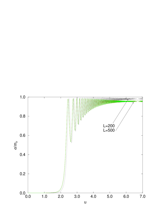
Figure 6: Evolution of $\sigma$ as a function of $u$ for two different values of the dimensionless box length.

In fig. 7 we show how the evolution of $\sigma$ depends on the time step $du$. We see that once we have a time step $du=0.00004$ then our results are insensitive to any further reduction in time step.

Figure 7: Evolution of $\sigma$ as a function of $u$ for different values of $du$.

.

In fig. 8 we see how the approach to the continuum value of ${\sigma\over m_{f}}=1$ depends on the number of Fourier modes. We see that at late times there is still some depedence of the asymptotic value on the number of modes.

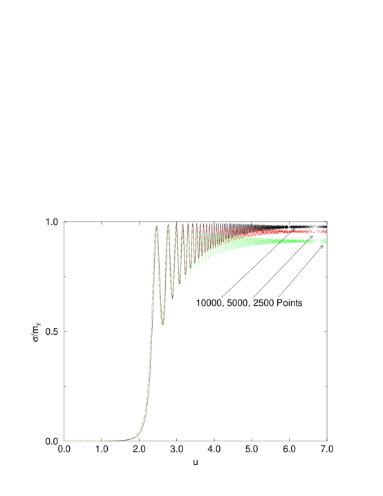
Figure 8: Evolution of $\sigma$ as a function of $u$ for increasing numbe of Fourier modes.

.

Another issue we would like to address here is the dependence of the evolution on the initial conditions chosen. We have seen that in LOLN, if we start with the fermion mass exactly zero, then the theory is non-interacting. Thus we must consider the massless theory as the limit of the massive theory, with the understanding that in higher order the fluctuations ignored in LOLN will make the equation for the fermion modes nontrivial even in the unbroken symmetry phase. To see that the theory actually approaches a limiting behavior, we considered initial condition where either the mass is small and not zero or the time derivative of the mass is non zero. The limiting theory is seen to be more readily accessed by choosing $\dot{\sigma}=0$ and gradually letting $\sigma\rightarrow 0.$ For ${\sigma_{0}\over m_{f}}\leq 10^{-7}$ the transition point changes little. We illustrate this graphically below. Figure 9 displays the time evolution for different initial values of $\dot{\sigma}$. Figure 10 displays the time evolution for different initial values of $\sigma$. As we go to bigger initial values of $\sigma$ or $\dot{\sigma}$ the transition is more a gradual crossover rather than a sharp transition.

Figure 9: Evolution $\sigma$ as a function of $u$ for 3 different values of $\dot{\sigma}$. First figure is for $\dot{\sigma}=10^{-1}$ , second figure is for $\dot{\sigma}=10^{-4}$ and third figure is for $\dot{\sigma}=10^{-5}$.

Figure 10: Evolution $\sigma$ as a function of $u$ for 3 different values of $\sigma$. First figure is for $\sigma=10^{-2}$ , second figure is for $\sigma=10^{-3}$ and third figure is for $\sigma=10^{-7}$.

Based on this discussion, in the simulations presented below, we will canonically use the values $du=0.00004$, $\tilde{L}=500$, $N=5000$, and $\sigma=10^{-7}$.

VIII.1 Proper time evolution of $\sigma$, $N_{\pm}$,$T$ and $\mu$

We have determined ${\tilde{\sigma}}(u)$ in terms of the mode functions using two different methods: the explicitly renormalized equation, eq. (77) and the combined set of eq. (71) and eq. (76). The latter set of equations also allows one to check whether one has included enough mode functions for the coupling constant to flow logarithmically as in the continuum limit. In the previous section we have discussed how these numerical results depended on various discretization parameters as well as the small initial value of the the explicit symmetry breaking. From the mode functions, using eq. (124), one determines the Bogoliubov coefficints and then determines $N_{\pm}(k,u)$ from eq. (127). By comparing eq. (127) with an equilibrium paramatrization:

$$N_{\pm}(k,u)\equiv\left(1+\exp[{\omega_{k}(u)\mp\mu(k,u)\over T(k,u)}]\right)^{-1}~{},$$ (139)

where $\omega_{k}=\sqrt{{k_{\eta}^{2}\over\tau^{2}}+\sigma^{2}}$ we then obtain two equations for the two parameters $T(k,u)$ and $\mu(k,u)$ as a function of $k_{\eta}$. When these quantities are independent of $k_{\eta}$ this defines the proper time evolving temperature and chemical potential. Some indication that an equilibrium parameterization is possible in a 1+1 dimensional field theory evolution in the LOLN approximation was already shown in the work of Aarts et. al. ref:Aarts . In our simulation we find that $T$ and $\mu$ are independent of $k_{\eta}$ (except at high momentum) until the system undergoes the chiral phase transition. A typical example of the dependence of $T$ and $\mu$ on $k_{\eta}$ is shown in fig. 11. For these initial conditions the phase transition occurs near $u=2$. The connection between $k_{\eta}$ and $j$ of the plot is given in eq. (88), namely: $k[j]=2\pi(j-1/2)/L.$

Figure 11: Effective temperature and chemical potential as a function of $k_{\eta}$ for u=1.0 and u=2.5

Because the system goes out of equilibrium after the phase transition, determining $T$ and $\mu$ in that regime is somewhat arbitrary and we use a value averaged over $k_{\eta}$. As we have shown earlier, if the system evolves in local thermal equilbrium in a massless phase, then $T$ falls as $1/\tau$. If there is also chemical equilibrium then $\mu$ falls identically to $T$. We will find this is precisely true before the phase transition when there is a second order phase transition. For the first order transition $\mu$ appears to fall faster than $T$. We also showed that if local chemical and thermal equilbrium are maintained, then the spectrum of particles and antiparticles when plotted against the dimensionless momentum $k_{\eta}=k\tau$ should be independent of $\tau$. Thus any change in this spectra is an indication of the system going out of equilibrium. We expect because of the latent heat released during a first order transition that the distortion of the spectra would be greatest in that case which is what we will find below. For the time evolution of the single particle distribution, we pick two time $u=1.5$ and $u=2.5$ which are before and after the phase transition.

Let us now focus on the four initial conditions described earlier and look simultaneously at the time evolution of the order parameter $\sigma$, $T$ and $\mu$ as a function of $u=\ln{m_{f}\tau}$. We separately plot the evolution of $N_{\pm}(k_{\eta},u)$. In all these plots all dimensionful parameters are scaled by the mass of the Fermion $m_{f}$ in the broken symmetry vacuum state.
case (1) $\mu_{0}=.2;T_{0}=.3$ – no phase transition
Here we start below the phase transition so that the Fermions initially have non-zero mass. The results for the order parameter $\sigma$ as well as for $T$ and $\mu$ are displayed in Fig. 12.

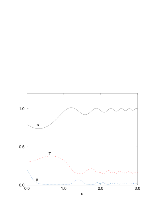
Figure 12: Typical evolution of $\sigma/m$, $\mu$ and $T$ as a function of $u$ for initial conditions below the phase transition temperature

We see here that although the chemical potential goes to zero as the plasma expands, after $u=1.5$, all the parameters become relatively independent of $u$ and are defined by an equilibrium freezeout temperature of approximately $.2m_{f}$.

For the broken symmetry case, the plasma essentially stays in equilibrium throughout the evolution in that the proper time evolving $N_{\pm}$ is relatively independent of $\tau$ and maintains its Fermi-Dirac shape. This is seen in Fig. 13.

Figure 13: Evolution of $N_{\pm}$ as a function of $u$ when there is no phase transiton. The momentum displayed is $k_{\eta}=k\tau$.

case (2) $\mu_{0}=.5;T_{0}=.5$ – second order phase transition
The results for starting in the “unbroken” mode and traversing a second order phase transition are shown in Fig. 14.

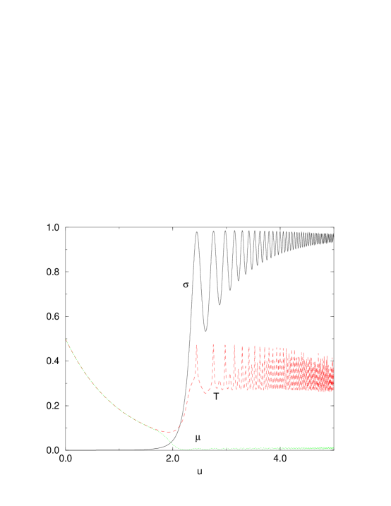
Figure 14: Evolution of $T$,$\mu$ and $\sigma$ as a function of $u$ for second-order phase transition

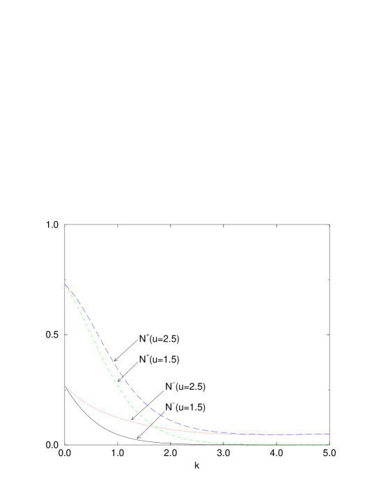
Figure 15: Evolution of $N_{\pm}$ as a function of $u$ when there is a second order phase transiton. The momentum displayed is $k_{\eta}=k\tau$

We notice that $\sigma(\tau)$ shows a sharp transition during evolution from the unbroken mode ($\sigma=0$) to the broken symmetry mode. Before the phase transition the temperature falls consistent with the equation of state $p=\epsilon$. The chemical potential follows the temperature in that regime which means the system is also in chemical equilibrium. After the phase transition, the chemical potential goes to zero wheras the temperature freezes out at a $T\approx.35m_{f}$. After the phase transition, there is now a mass scale $m_{f}$ which leads to oscillations of $\sigma$ around the final vacuum value. As discussed earlier, to obtain non-trivial dynamics we chose a small explicit symmetry breaking parameter $\sigma/m_{f}=10^{-7}$.

Going through a second order phase transition does produce a noticable effect in distorting the Fermi-Dirac distribution as shown in Fig. 15

case (3) $\mu_{0}=.6;T_{0}=.32$ –traversing the tricritical point
The results for this numerical simulation are shown in Fig. 16.

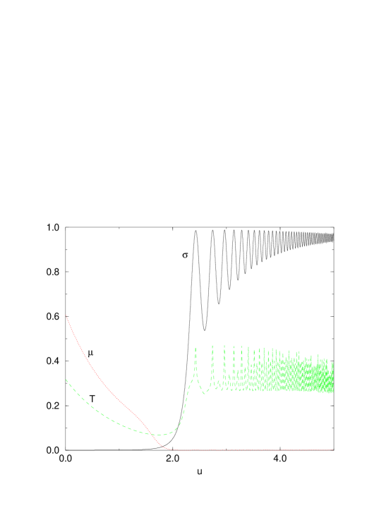
Figure 16: Evolution of $T$,$\mu$ and $\sigma$ as a function of $u$ passing throught the tricritical point

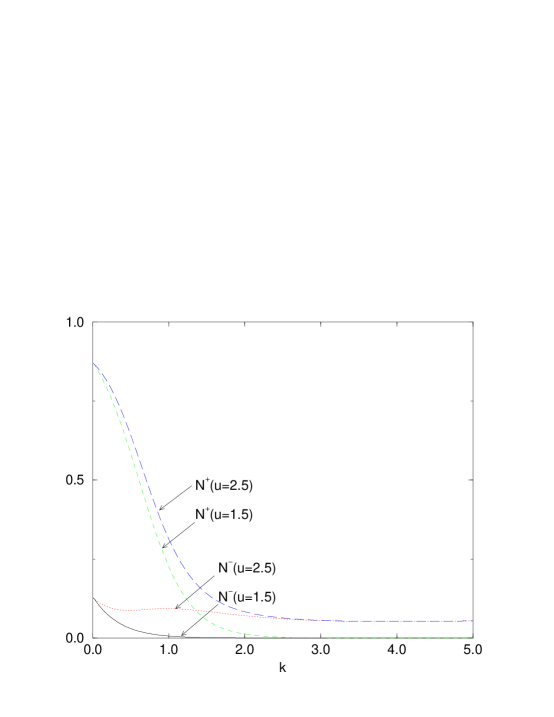
Figure 17: Evolution of $N_{\pm}$ as a function of $u$ when one traverses the tricritical point.The momentum displayed is $k_{\eta}=k\tau$.

We notice that $\sigma(\tau)$ again shows a sharp transition during evolution from the unbroken mode ($\sigma=0$) to the broken symmetry mode and again the temperature falls consistent with the equation of state was $p=\epsilon$ before the transition and frezes out again with $T\approx.35m_{f}$. However the chemical potential in this case falls faster than the temperature. When one traverse the tricritical point the distortion of the Fermi-Dirac distribution is greater than for the second-order phase transition case as shown in Fig.17.

case (4) $\mu_{0}=.8;T_{0}=.3$ –first order phase transition
Finally we present results when we start in the unbroken mode and go through a first order phase transition. First we display the $\sigma,\mu,T$ in Fig. 18.

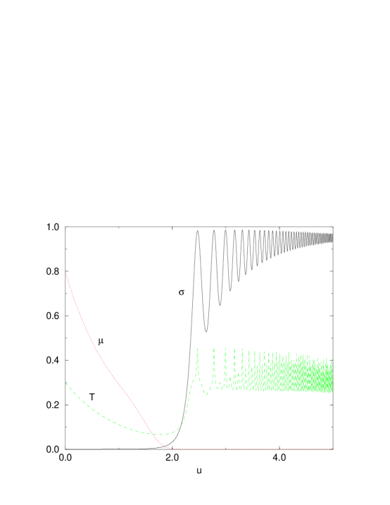
Figure 18: Evolution of $T$,$\mu$ and $\sigma$ as a function of $u$ passing through first order phase transiton.

The results for these variables are qualitatively the same as for going through the tricritical point, however the chemical potential falls even faster in this case. By comparing the three different cases where there is a phase transition, we find among the parameters $T$,$\mu$ and $\sigma$, only the behavior of the chemical potential $\mu$ is effected by the order of the phase transition. The chemical potential falls as ${1\over\tau}$ for the second order phase transition and faster for the first order transition suggesting a deviation from local chemical equilibrium.

The greatest change in the Fermi-Dirac Distribution also occurs for the first order transition. This is a result of converting (the small amount of) latent heat into pair production and is seen in Fig. 19.

Figure 19: Evolution of $N_{\pm}$ as a function of $u$ when there is a first order phase transiton.

As we recall from our study of the effective potential, for the GN model the first order phase transition is not very strong. The difference in energy density between the false and true vacuum (measured in units of $m_{f}^{-2}$) is ${1\over 4\pi}$, wheras the height of the barrier at phase coexistence (seen from Fig. 2) is less than 10 % of this difference.

VIII.2 Numerical results for the energy density and pressure

In local equilibrium in the massless phase, we have shown that the equation of state would be $\epsilon=p$ and these quantities would fall as $1/\tau^{2}$ as shown in Fig. 5. In our field theory simulations, we will find that this behavior is followed until the phase transition occurs. After that the energy density and pressure diverge from each other and oscillate. These oscillations would be damped if we were to go beyond mean field theory and include hard scatterings between the Fermions. After the phase transition we find that the energy density oscillates around the true broken symmetry values discussed earlier, namely

$$\epsilon_{0}=-{1\over 4\pi}~{}.$$

For these simulation we will assume the initial conditions described earlier and plot the renormalized energy density and pressure described by eq. (100) and eq. (107). Starting in the massless (unbroken symmetry) regime we will find $p=\epsilon$ and this fall off pertains until one goes through the phase transition, after which the system is no longer in local equilibrium. In Fig. 20 we show the result of plotting the energy density $\epsilon(u)$ and pressure $p$ for three initial conditions.

Figure 20: Evolution of $p$ and $\epsilon$ as a function of $u$ for three initial conditions.

In Fig. 21 we plot the pressure and energy density for the three initial data (cases (2),(3),(4) ) for which there is a phase transition. We see that before the phase transition, $p$ tracks $\epsilon$. After the transition, the system goes out of equilibrium and then oscillates about its vacuum value because there are no damping mechanisms.

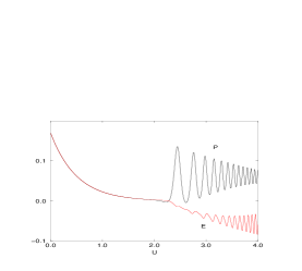
Figure 21: From left to right: evolution of the pressure and energy density as a function of $u$ when there is a second order phase transition; evolution of the pressure and energy density as a function of $u$ when the trajectory passes through a tricritical point; evolution of the pressure and energy density as a function of $u$ when there is a first order phase transition.

IX “Pion” correlation function

One interesting question we can ask is how correlation lengths change as we go through the phase transition. In our toy model there is no physical pion bound state in our approximation, but we still can define an effective field for the pion and study the spatial dependence of the pion green’s function. Other correlation functions one can study in a similar fashion are the density fluctuations as well as the condensate fluctuations.

We can define an effective (neutral) pion field via

$$\pi(x)\equiv c\bar{\psi}_{i}(x)i\gamma^{5}\psi_{i}(x)~{},$$ (140)

where $c$ is a constant. Using our mode expansion we find that

$$\langle:\bar{\psi}i\gamma^{5}\psi:\rangle ={2\over\tau^{2}}\langle[\phi_{i}(x)^{{\dagger}},\gamma^{3}\phi_{i}(x)]\rangle$$ (141)

$$=\int dk_{\eta}k_{\eta}[2-N_{+}(k)-N_{-}(k)]{d\over du}|f_{k}|^{2}~{}.$$

Because the integrand in eq. (141) is odd, the expectation value is zero (otherwise there would be spontaneous breakdown of parity).

For the equal time correlation function in LOLN, we obtain the usual Fermion self energy loop. This depends on the time evolving distribution of Fermions and anti-Fermions. Apart from an overall constant one can write the connected correlation function in the form:

$$D(\eta-\eta^{\prime};\tau)\equiv\langle\pi(\eta,\tau)\pi(\eta^{\prime},\tau)\rangle_{c}={1\over\tau^{4}}{\rm Tr}[\gamma^{3}S(\eta-\eta^{\prime};\tau)\gamma^{3}S(\eta^{\prime}-\eta;\tau)]~{},$$ (142)

where at equal times, the propagator is just

$$S(\eta,\eta^{\prime};\tau)_{\alpha\beta}=\langle[\phi_{\alpha}(\eta,\tau),\phi^{{\dagger}}_{\beta}(\eta^{\prime},\tau)]\rangle~{}.$$ (143)

Here $\alpha,\beta$ take on the values $\{1,2\}$ and are the spinor indices. Using the mode expansion eq. (3.20) we find that the equal time propagator can be written as

$$S(\eta,\eta^{\prime};\tau)_{\alpha\beta} =\int{dk_{\eta}\over 2\pi}e^{ik_{\eta}(\eta-\eta^{\prime})}\left[\left(1-2N_{+}(k)\right)\phi^{+}_{k\alpha}(\tau)\phi^{{\dagger}+}_{k\beta}(\tau)\right.$$ (144)

$$+\left.\left(2N_{-}(k)-1\right)\phi_{k\alpha}(\tau)\phi^{{\dagger}-}_{k\beta}(\tau)\right]~{}.$$

We could also have use the mode expansion in terms of adiabatic mode functions, eq. (7.1) and obtained an expression for the equal time propagator in terms of the time evoloving adiabatic number distributions.

Evaluating the trace we obtain

$$\tau^{4}D(\eta-\eta^{\prime};\tau)=\int{dk\over 2\pi}{dq\over 2\pi}e^{i(k-q)(\eta-\eta^{\prime})}D(k,q;\tau)~{},$$ (145)

where

$$D(k,q) =([1-2N_{+}(k)][1-2N_{+}(q)]+[1-2N_{-}(k)][1-2N_{-}(q)])F_{1}(k,q)$$ (146)

$$+([1-2N_{+}(k)][1-2N_{-}(q)]+[1-2N_{+}(q)]~{}.[1-2N_{-}(k)])F_{2}(k,q)$$

and

$$F_{1}(k,q;\tau)=|f_{k}|^{2}|f_{q}|^{2}\{(k\Delta_{q}+q\Delta_{k})^{2}+[k({\tilde{\Omega}}_{q}+{\tilde{\sigma}})-q({\tilde{\Omega}}_{k}+{\tilde{\sigma}})]^{2}\}~{},$$ (147)

and

$$F_{2}(k,q;\tau) =|f_{k}|^{2}|f_{q}|^{2}([kq-\Delta_{k}\Delta_{q}+({\tilde{\Omega}}_{k}+{\tilde{\sigma}})({\tilde{\Omega}}_{q}+{\tilde{\sigma}})]^{2}$$ (148)

$$+[\Delta_{k}({\tilde{\Omega}}_{q}+{\tilde{\sigma}})+\Delta_{q}({\tilde{\Omega}}_{k}+{\tilde{\sigma}})]^{2})~{}.$$

If we were solving a $3+1$ dimensional 4-fermion model with actual pion composite particles we would now be in a position to determine the single particle distribution function for the pions from the Wigner distribution functions which is just a particular Fourier transform of the Green’s function over the relative coordinate.

In Figs. 22, 23 we plot $\tau^{4}D(\eta,\tau_{f})$ as a function of $\eta$ for cases (2) and (4) for a sequence of times starting near the onset of the phase transition.

Figure 22: Evolution of the Correlation function as a function of time. This is for a first order transition.

Figure 23: Evolution of the Correlation function as a function of time. This is for a second order transition.

X Conclusion

In this paper we have performed simulations in the Gross-Neveu model of an expanding plasma of fermions and antifermions. We have chosen inital conditions where the density matrix is described by single particle distribution functions pertinent to a plasma initially in local thermodynamic and chemical equilibrium. The model was treated in the leading order in large $N$ approximation. In this approximation the phase diagram at finite chemical potential and temperature shares features with that of massless 2-flavor QCD. We found that if we start in the unbroken symmetry phase, the system remains in equilibrium until the phase transition and then goes rapidly out of equilibrium as the phase transition is traversed. The effects of the phase transition are greatest when we traverse a first order phase transition and are most noticable in the anti-fermion distribution function. If these effects survive hard scatterings then this should have an effect on the distribution of dileptons, just as the overpopulation of soft pions during DCC production effected the distruibution of dileptons as discussed by us earlier slansky . We also find that before the phase transition, the system behaves identically to an ideal fluid in local thermal equilibrium with equation of state $p=\epsilon$. After the phase transition, the system quickly reaches its true broken symmetry vacuum value for the fermion mass and for the energy density. Since hard scatterings are ignored in this approximation, the competition between the expansion of the plasma and the competing process for re-equilbration could not be studied here. Also by restricting our simulations to inhomogeneities which are boost invariant, we were not able to look at bubble nucleation. In future investigations we will attempt to remedy the shortcomings just mentioned. We will perform mean field simulations for inhomogeneous initial conditions which we discussed before inhom and which have already been undertaken in scalar field theory in 1+1 dimensions ref:Aarts . There are also now two different approaches for going beyond $1/N$ based on Schwinger Dyson equations which we hope we can implement to study whether rethermalization can occur for the type of expansion expected following a heavy ion collision. These approaches are based on different approximations for the generating functional for the 2-PI irreducible graphs ref:beyond ref:berges and should allow us to study the question of rethermalization. We also want to extend our simulation to a more realistic O(4) 4-Fermi Model in $3+1$ dimensions so that we can directly study the effect of the phase transition on pion correlation functions.

A  spinor bases, Dirac matrices

We will choose for convenience the following representation for the matrices $\gamma^{0}$ and $\gamma^{3}$

$$i\gamma^{0}=\left(\matrix{1&0\cr 0&-1\cr}\right)$$ (A.1)

$$\gamma^{3}=\left(\matrix{0&1\cr 1&0\cr}\right)$$

Thus the spinor eigenstates of $i\gamma^{0}$ are

$$\chi^{+}=\left[\matrix{1\cr 0\cr}\right]$$

$$\chi^{-}=\left[\matrix{0\cr 1\cr}\right]$$

In terms of this explicit representation we find that the momentum space wave functions have the form:

$$\phi^{+}_{k} =\left[({\tilde{\Omega}}_{k}+{\tilde{\sigma}}-i\Delta_{k})\chi^{+}-ik_{\eta}\chi^{-}\right]f^{+}_{k}$$

$$\phi^{-}_{k} =\left[({\tilde{\Omega}}_{k}+{\tilde{\sigma}}+i\Delta_{k})\chi^{-}-ik_{\eta}\chi^{+}\right]f^{-}_{k}$$ (A.2)