Are High Energy Heavy Ion Collisions similar to a Little Bang, or just a very nice Firework?

Abstract

The talk is a brief overview of what we recently learned about excited hadronic matter from heavy ion collisions. The central issue is that the systems produced do exhibit macroscopic behavior, it flows and we start getting some idea about its effective Equation of State (EoS). More specifically, we concentrate on elliptic flow, from SPS to RHIC energies, as well as on particle composition and fluctuations. Note that a pressure and the rate of fluctuation relaxation (discussed at the end) are ultimately a measure of a collision rate in the system we would like to understand.

1 Flows

1.1 QCD phase transition and flows

We start with general questions, such as: Do we produce excited matter with sufficiently large scattering rate able to ensure local equilibration? If so, what is its EoS and whether it is close to results obtained in lattice simulations? How one can tell the Bang from a Fizzle, experimentally? There are 3 effects one can discuss: (i) longitudinal work; (ii) radial transverse flow; and (iii) elliptic flow. We address two last ones below.

Before we go to specific description of concepts and data on flow, let us discuss in general why we think that rather different phenomena at AGS/SPS and RHIC energy domain can nevertheless be described in a unified way by hydro+cascade model. Those types of models are the only ones known, which can incorporate correctly the fact that hadrons and partons live in different vacua, separated by significant “bag term” in EoS. This phenomenon generates soft “mixed phase”, in which energy density $\epsilon$ grows but temperature T and pressure p do not. Purely cascade models with partons/hadrons miss this central point, and therefore have very unrealistic EoS.

The Hydro-to-Hadrons Model [1] include hydro plus transfer to hadronic cascade (RQMD), in order not to worry about freeze-out of different species, resonance decays etc. The transfer is smooth enough because the effective EoS of RQMD and our hadronic matter is about the same.

At SPS the evolution starts close to rather soft “mixed phase” (as lattice thermodynamics tells us), then proceeding to stiffer pion gas: therefore most of the radial expansion is pion-driven and happens very late. There are many proves of that: one [2] is that $\Omega^{-}$ which participate little in hadronic rescattering practically do not have it.

Let us first characterize flows in general. At RHIC we start well above the QCD phase transition, and so expect the so called “QGP push”, then softer mixed phase, and finally a stiff hadronic phase again. (Now $\Omega^{-}$ is expected to flow more!)

In non-central collisions at SPS the initial almond for $b\sim R$ collisions retains basically the same almond shape: matter does not move till the final velocity $v_{t}\approx 0.5$ is only obtained close to the end of the expansion. At RHIC the initial almond is transformed into a completely different object called the “nutcracker” [8], which consists of two separated shells of matter and a small “nut” in the center. It happens by the time 8-10 fm/c, and then shells continue to move out in hadronic phase, slowly dissolving.

Radial flow is usually characterized by the slope parameter T: $dN/dp_{t}^{2}dy\sim exp(-m_{t}/T),m_{t}^{2}=p_{t}^{2}+m^{2}$. T is $not$ temperature: it incorporates random thermal motion and collective transverse velocity. Its prediction for various EoS (marked by latent heat, say LH8 means latent heat 800 $MeV/fm^{3}$, see fig.1a) is shown in the following figure , for protons and pions versus basically collision energy expressed in terms of multiplicity, see fig.1b. One can see that different EoS show different growth, although picture is rather simple: the softer the EoS the less flow.

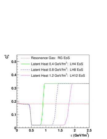
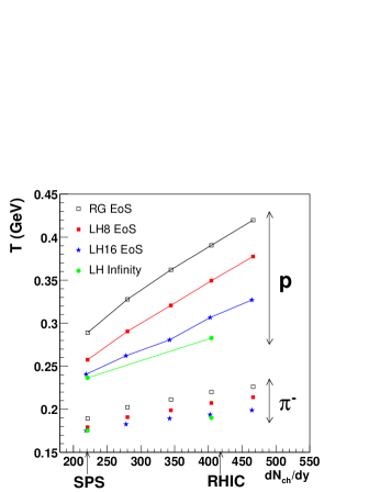
Figure 1: The speed of sound for a set of EoS used (a) and resulting transverse mass slope T (b) versus mid-rapidity (y=0) charged particle multiplicity, for AuAu collisions with b=6.

1.2 Elliptic flow

If there is no correlation between space and momentum, there is no elliptic flow. For example, $any$ model like [4] in which transverse momentum increase in AA is due to initial state interaction, like in pA collision, cannot have elliptic flow. Indeed HIJING parton model [5] without rescatterng (an example of the model which produce a “firework” type final state) has nearly zero (actually slightly negative) $v_{2}$. String models like UrQMD [6] and RQMD itself also do not produce pressure at early time, and predicted respectively $smaller$ $v_{2}$ at RHIC than at SPS Those are eliminated, as soon as the first STAR data [3] have shown that at RHIC $v_{2}$ is in fact twice larger than at SPS!

But hydro knows about geometry of the excited system: the pressure gradient is mostly along the narrow part of the almond. The elliptic flow is quantified experimentally by the elliptic flow parameter $V_{2}=\langle cos(2\phi)\rangle$

The energy dependence of $V_{2}$ does not appear to be simple (in contrast to radial flow). Furthermore, we have found that if one is making EoS softer the $v_{2}$ decreases non-monotonously, first decreasing and then increasing again. It means for a given experimental value of $V_{2}$ there are two possible scenarios, we called the “QGP push” and “burning almond”. In the first case the initial almond transfers to nutcracker, in which spatial anisotropy decreases and even change sign. In the second, the almond dries out, and spatial anisotropy actually grows. So, in order to answer the question whether the “QGP push” scenario we are waiting for is or is not the case, some further studies are needed. In particular, the scan in RHIC energies downward would be very useful.

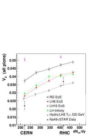
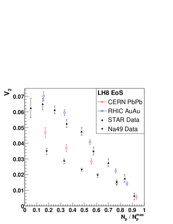
Figure 2: (a) The elliptic flow parameter $V_{2}$ versus multiplicity at b=6 fm, for different EoS. (b) $V_{2}$ is now plotted versus impact parameter b, described experimentally by the number of participant nucleons, for RHIC STAR and SPS NA49 experiments. Both are compared to our results for EoS LH8.

Fig.2b shows data as a function of impact parameter. One can see that the agreement becomes much better at RHIC. Furthermore, one may notice that deviation from linear dependence we predict becomes visible at SPS for more peripheral collisions with $N_{p}/N_{p}^{max}<0.6$ or so, while at RHIC only the most peripheral point, with $N_{p}/N_{p}^{max}=0.05$ show such deviation. This clearly shows that hydrodynamical regime in general works much better at RHIC. On the other hand, a models of single re-scattering (e.g. [7]) which approximately describes peripheral SPS data is completely inconsistent with this linear rise, seen both at SPS and RHIC.

2 Matter composition

2.1 Strangeness

The discussion of the role of s,c quarks in excited hadronic matter has a peculiar history. In the first paper addressing the subject [9] it was argued that QGP with $T\sim 500\,MeV$ should quickly equilibrate even charm, because of high rate of gluon-induced processes, and suggested to use it as a QGP signature. As for strangeness, the $m_{s}$ was considered to be too small to be useful for that purposes. However later, Rafelski et al [10] had nevertheless suggested that the strangeness enhancement for exactly that role. The experiments at AGS/SPS indeed found lager strangeness per participant baryon (or per pion) in AA collisions than in pp, which is more pronounced for hyperons and especially for $\Omega^{-}$. However, the following two features has been also found. First, strangeness enhancement started at very low energies, at AGS. Second, its magnitude basically described by the statistical model (see e.g.[11]), by an equilibrium at $T\approx 170\,MeV$ and $\mu_{b}$ depending on the collision energy. From this point of view people rather called a phenomenon a “disappearance of strangeness suppression”, which has been present in pp.

But even this interpretation has been recently challenged in [12]. Already 25 years ago the issue of correct account for strangeness in small statistical systems has been addressed in [14]. The main point is, the usual statistical expressions say for $K/\pi$ ratio, being the ratio of integrated Bose distribution, is only valid if the average particle number $<N_{K}>\gg 1$. If it is not so, exact strangeness conservation should be enforced while considering all possible states of the system, say containing $KK$ pairs, etc. As a result, $<N_{K}>$ depends on volume (or $<N_{\pi}>$) quadratically, till $<N_{K}>\sim 1$. In $\bar{p}p,pp$ collisions at few GeV range the data were in perfect agreement with this prediction already in 1975 [14]. We are however still lacking a demonstration of where that happens for say $\Xi,\Omega$: even most peripheral data at SPS do not show a predicted transition to small-volume regime, their ratio to multiplicity remains flat. Probably lighter ions are needed to see it.

In summary: whatever strange it may appear to us, composition of hadrons, including strange ones, seem to be thermal $both$ in AA (at AGS/SPS energies) and pp collisions. In the latter case it is believed to come from string fragmentation: so AA can either be also string-based, or come from QGP, which (by coincidence?) have a $T_{c}$ value which mimic string decays.

2.2 Solving the anti baryon puzzle

Anti-baryon ratios, like many others, can be rather accurately characterized by the so-called chemical freeze-out stage with a common temperature $T_{ch}$ $\mu_{B,ch}$ (values depend on collision energy). However, the kinetics of other particles and anti-baryons cannot be the same. The number of pions, kaons, etc. are not subject to significant changes when the system evolves from $T_{ch}$ to $T_{th}$: thus ’over-saturation’ appears, the effective pion fugacity

$$z_{\pi}=exp(\mu_{\pi}/T_{th})\approx 1.6-1.9$$

The situation for antibaryons is different because the pertinent annihilation cross section is not small, $\sigma_{p\bar{p}\to n\pi}\simeq 50$ mb. The time in which a give antinucleon is eaten is only

$$\tau_{ch}=\frac{1}{\sigma_{ann}\ \rho_{B}\ v_{th}}\simeq 3~{}{\rm fm/c}$$

and so naively one might expect most of the antiprotons to be annihilated, and various transport calculations ( ARC, UrQMD) have indeed been unable to account for the measured number, falling short by significant factors. Speculations have been put forward: either a reduction of the annihilation rate or an enhanced production.

Inverse reactions, ignored in event generators, are however not small [15]

$${\cal R}_{th}=|{\cal M}_{n}|^{2}\exp[-(E_{p}+E_{\bar{p}})/T]\ \left[z_{p}\ z_{\bar{p}}\ -z_{\pi}^{n}\right]$$

The condition that this reaction goes on implies [15]

$$z_{\bar{p}}=(z_{p})^{-1}{\langle z_{\pi}^{n}\rangle}$$

which leads to predictions consistent with the experimental value of $N_{\bar{p}}/N_{p}=(5.5\pm 1)\%$ (na44). Note that it is very multi-pion reaction, with n=6-7.

After the paper by Rapp and myself, C.Greiner and S.Leupold [16] generalized it further, to $\bar{Y}+N\leftrightarrow n\pi+K$ where $Y=\Sigma\Xi,\Omega$. Similar multi-meson annihilation can also explain the long-standing puzzle about multiple production anti-hyperons.

2.3 Charm and $J/\psi$ suppression

Charm production at SPS is due to hard gg collisions, which are obviously able to produce somewhat larger amount of it, compared to its equilibrium value at $T=170\,MeV$. Direct measurements are still in the future, but we should hardly expect any surprises here. (The NA50 medium mass dilepton excess fits nicely to thermal dilepton rate [13], so I do not think it is a charm enhancement.)

Do $J/\psi,\psi^{\prime}$ we observe in AA collisions know about hadronic matter which surrounds it, or their cross section is too small and too absorptive (leading to $\bar{D}D$ pairs) that all of them we see just jump intact directly from the primary production point? The latter remains the prevailing view in the field, although it has been challenged lately.

Although $\psi^{\prime}/J/\psi$ ratio starts decreasing at rather peripheral collisions/small A, as larger radius of $\psi^{\prime}$ suggests larger cross section, it then stabilizes at $\psi^{\prime}/J/\psi\approx 0.05$. Furthermore, as noticed in [17], this number is consistent with the same $T\approx 170\,MeV$ which fits all other ratios. This leads to an idea that the observed $\psi^{\prime}$ is excited from $J/\psi$.

Much more radical idea has been put forward in [18]: the number of $J/\psi$ itself is in agreement with the statistical model, provided the total charm fugacity is fixed to the parton model production. If it is not a coincidence, it then implies that $J/\psi$ may in fact be created from the same heat bath as all other hadrons. If so, the individual string scenario is of course out of the window, and the QGP scenario (with some extra charm added to it) is in.

Much more charm is expected at RHIC: it makes recombination of floating charm pairs into charmonium states even more likely. The issue has been studied in recent paper [20]: the conclusion is that we should in fact expect a charmonium enhancement at RHIC.

3 Event-by-event Fluctuations

3.1 Current SPS data versus theory

Unlike pp collisions, the AA ones demonstrate small fluctuations of Gaussian shape, as measured e.g. by NA49. It is basically a consequence of a basic theorem of probability theory, roughly stating that any distribution with a maximum in high power becomes Gaussian. Still, it is quite striking how far this Gaussian goes: no deviations from it is seen for few decades, as far as data go. No trace of any large fluctuations, DCC or other bubbles, and all events with the same impact parameter are basically alike.

The question then is whether the $widths$ of those Gaussians is understood. The short answer is yes. Somewhat longer answer is that one should separate [21] fluctuations of two types, of intensive or extensive variables. The latter is e.g. total charge multiplicity: it obtains about equal contributions from the initial (due to fluctuations in spectators) and final stage (resonances). The former (e.g. particle ratios like $\pi^{+}/\pi^{-}$) are well described by resonances at freezeout.

To give some example, consider fluctuations in charged multiplicity measured by NA49 at 5% centrality:${<\Delta N_{ch}^{2}>\over<N_{ch}>}\approx 2.0$, while Poisson statistics (independent production) gives 1 in the rhs.

Statistical fluctuations in a resonance gas increase the rhs. Example: if all pions would originate from $\rho^{0}\rightarrow\pi^{+}\pi^{-}$, and rho would be random, then the rhs would be 2. Account for equilibrium composition lead however to the Gaussian width of only about 1.5 [21]. Correlations coming from fluctuation in the number of participants further increase it [22]: see the comparison in the figure 3:

Figure 3: The calculated multiplicity distribution from our model (solid line) is compared to the observed one (points).

Good examples of intensive variable fluctuations are those in the mean $p_{t}$ (in an event) or in electric charge Q (same as of the $\pi^{+}/\pi^{-}$ ratio). Resonances again: e.g. $\rho^{0}\rightarrow\pi^{+}\pi^{-}$ does not lead to Q but contribute to multiplicity $Q^{2}/<N_{c}h>\approx.7-.8$, not 1 as for Poisson. It is what is actually observed for central collisions by NA49.

3.2 Can “primordial” fluctuations be seen?

In order to do so, we need a telescope looking back into the past, through the clouds of hadronic matter. How to make it has been recently suggested in refs [23]. The idea is to use long-wavelength fluctuations of conserved quantities, which have slow relaxation. Example: primordial fluctuations in microwave background give us “frozen plasma oscillations” at Big Bang. Can we find similar signal in the “Little Bang”? Yes: if relax.time is longer than lifetime of hadronic stage the fluctuations we would see are “primordial ones”, from the QGP which are factor $\sim 3$ smaller.

Quantitative studies have been recently done by Stephanov and myself [24]. Fluctuations are governed by Langevin eqn

$${\partial_{\tau}f}=\gamma(\tau)\,\partial^{2}_{y}f+\xi(y,\tau)$$

and we calculated $\gamma(\tau)$ for pions in collisions. Basically we found that at RHIC/SPS pion diffuse during hadronic stage by about 2 units of rapidity. NA49 data we had are in acceptance $\Delta y=2$ and show perfect agreement with equilibrium resonance gas. STAR detector may have $\Delta y=4$ and additional deviation from 1 by about 20% - quite observable.

Baryon number fluctuations idea cannot work because we do not see neutrons.

4 Summary

• – If hydro description plus lattice-like EoS makes sense, we found that the QCD phase transition plays different role at AGS/SPS and RHIC: it makes the EoS effectively soft in the former case but stiff at high energy, providing early “QGP push”.

• – Collective flow, especially its elliptic component, is very robust measure of the pressure in the system. STAR data at RHIC, which demonstrate increase of elliptic flow by factor 2, contradicts to string-based models and also mini-jet models without rescattering. Hydro-based model, especially H2H model with hadronic cascades, can describe these data very accurately. Still two solutions seem to be possible, one with strong QGP push (predicted by lattice-based EoS) and another with longer-time burning.

• – Strangeness seem to be well equilibrated in any collisions, and thus is not a QGP signature. Whether $J/\psi$ can obtain significant contribution from equilibrated charm at SPS is strongly debated: it should however be the case at RHIC.

• – Event-by-event fluctuations are mostly due to final state interaction between secondaries, and available data are in agreement with equilibrium resonance gas calculations.

• – Potential observations of “primordial charge fluctuations” are limited by their relaxation time, mostly due to pion diffusion in rapidity. The outlook depends on experimental acceptance: available calculations suggest that wide STAR acceptance can be sufficient to see 10-15 percent modification of charge fluctuations.

References

- [1] D.Teaney, J. Lauret and E.Shuryak, Collective Flows at RHIC as a Quark-Gluon Plasma Signal, nucl-th/0011058.
- [2] H. van Hecke, H. Sorge, N. Xu Nucl.Phys.A661:493-496,1999
- [3] K. H. Ackermann et al. [STAR Collaboration], “Elliptic flow in Au + Au collisions at s(N N)**(1/2) = 130-GeV,” nucl-ex/0009011.
- [4] A. Leonidov, M. Nardi, H. Satz, Z.Phys.C74:535-540,1997
- [5] Xin-Nian Wang, Miklos Gyulassy, Phys.Rev.D44:3501-3516,1991
- [6] M. Bleicher and H. Stocker, hep-ph/0006147.
- [7] H. Heiselberg and A. Levy, Phys. Rev. C59, 2716 (1999) [nucl-th/9812034].
- [8] D.Teaney and E.Shuryak,Phys. Rev. Lett. 83, 4951 (1999); nucl-th/9904006
- [9] E. Shuryak, Phys. Lett. 78B, 150(1978); Sov. J. Nucl. Phys. 28, 408(1978). Phys. Rep. 61, 71(1980);
- [10] P. Koch, B. Muller, J. Rafelski, Phys.Rept.142:167,1986
- [11] P. Braun-Munzinger, I. Heppe, J. Stachel, Phys.Lett.B465:15-20,1999.
- [12] K.Redlich et al, Phys.Lett.B486:61-66,2000: hep-ph/0006024
- [13] R. Rapp and E.V.Shuryak, Phys.Lett.B473:13-19,2000; hep-ph/9909348
- [14] E.V.Shuryak, PL 42B (1972) 357, Sov.J.Nucl.Phys.20,1975,295
- [15] R. Rapp and E.V.Shuryak,Resolving the Antibaryon Puzzle, hep-ph/0008326.
- [16] Carsten Greiner, Stefan Leupold, nucl-th/0009036
- [17] H.Sorge, E.Shuryak, I.Zahed Phys.Rev.Lett.79:2775-2778,1997, hep-ph/9705329.
- [18] P. Braun-Munzinger, J. Stachel,Phys.Lett.B490:196-202,2000; nucl-th/0007059.
- [19] M.I.Gorenstein et al, hep-ph/0010148.
- [20] R.L. Thews, M. Schroedter, J. Rafelski, hep-ph/0009090
- [21] M. Stephanov, K. Rajagopal, E. Shuryak,Phys.Rev. D60: 114028 ,1999; hep-ph/9903292.
- [22] G.V. Danilov, E.V. Shuryak, nucl-th/9908027.
- [23] M.Asakawa, U.Heinz and B.Muller, hep-ph/0003169, S.Jeon and V.Koch, hep-ph/0003168.
- [24] E.V.Shuryak and M.A.Stephanov, When can Long-Range Fluctuations be used as QGP signal? hep-ph/0010100.