We study the CP even trilinear neutral gauge boson vertices at one-loop in the context of the Standard Model and the Minimal Supersymmetric Standard Model, assuming two of the vector bosons are on-shell. We also study the changes in the form-factors when these two bosons are off-shell.

1 Introduction

Present measurements of the vector boson fermion couplings at the LEP and the SLC remarkably confirm the Standard Model (SM) predictions to a high degree of accuracy. While this strengthens our belief that the weak interactions are indeed governed by a non-abelian gauge theory, this hypothesis can be established only with an experimental confirmation of the non-abelian structure of the SM. Recently, some progress has been made in this direction in experiments at Tevatron [1] as well as at LEP-II [2]. However, the relatively low sensitivity of such experiments does not allow us to explore the couplings to the level of accuracy required to establish the gauge-theoretic nature of the SM. Nevertheless, one expects that the significantly improved facilities available at future experiments such as those at Linear Colliders (LC) [3, 4, 5], would allow us to corroborate the SM predictions in this sector. Furthermore, an accurate measurement of these cubic and quartic couplings could even act as a pointer to the existence of new physics beyond the SM even at energies lower than the corresponding production threshold.

Gauge invariance dictates that, within the SM, the trilinear neutral gauge boson vertices (TNGBVs) vanish at the tree level. However, one-loop corrections do generate small but non-vanishing values for these couplings. In composite models, on the other hand, these couplings can be significantly larger. In either case, one expects the strength of these couplings to have a nontrivial dependence on the momentum scale, a fact that may have a substantial bearing on their experimental signature.

At LEP (Tevatron), the $ZZ\gamma$ and $Z\gamma\gamma$ vertices are best studied in $Z\gamma$ production through processes such as $e^{+}e^{-}\rightarrow Z\gamma$ ($q^{+}q^{-}\rightarrow Z\gamma$). The anomalous coupling being of a non-renormalizable nature, a constant value of the same would, in general, lead to a cross section growing rapidly with energy. A momentum suppression, often expressed as a form-factor behaviour, can ameliorate the non-unitary nature though.

LEP-II [2] has been running at energies above $ZZ$ production threshold and for the first time $Z$ pairs are being obtained. During Run 2 at Tevatron and in future experiments at NLC or JLC, several hundreds of such $Z$ pairs will be produced. These could be profitably used to constrain both $ZZZ$ and $\gamma ZZ$ vertices. These anomalous couplings manifest themselves differently in the production of longitudinally or transversely polarised $Z$ bosons. Thus, for $ZZ$ production, helicity dependence of the decay distributions constitute an additional source of information. In this context it is worth mentioning that $WWV$ ($V=\gamma,\,Z$) vertex has been analysed in detail within SM and as well as in supersymmetric extension of it [6]. The measurement of $WWZ$ and $WW\gamma$ couplings at LEP-II has deservedly received considerable attention.

Since any significant modification due to new interactions beyond the SM constitutes a signal for new physics, some of these couplings have already been studied in the literature. However, very few of these papers [7, 8] treat the various qualitative and quantitative issues in an adequate manner. Therefore there exists a good motivation for a thorough and careful reexamination of the various contributions within the SM as well as within one of its most popular extension, viz. the Minimal Supersymmetric Standard Model (MSSM). While this work was being completed, the papers of Gounaris et al. [9, 10] appeared and we will comment on their results and make a comparison with our results later on.

In this paper we study the CP conserving couplings of TNGBVs. We organize our paper as follows. In section 2 we describe a general framework how the CP conserving form-factors can be derived from the general tensorial structure of the three-point functions. In section 3 we examine a general one-loop fermionic contribution to the three point functions $\gamma^{\star}Z\gamma$, $Z^{\star}Z\gamma$, $\gamma^{\star}ZZ$, $Z^{\star}ZZ$. In section 4 we calculate the SM contribution to these couplings and in section 5 we extend our study to MSSM. We study the changes in the form-factors in section 6 when the all the gauge bosons are put off-shell. Section 7 contains our conclusions.

2 Generic structure of form-factors

Let us consider the vertex: $V_{1}(p_{1\alpha})\,V_{2}(p_{2\beta})\,V_{3}(p_{3\mu})$ where $V_{i}\equiv\gamma,Z$ and $p_{1}+p_{2}+p_{3}=0$. The most general CP conserving tensorial structure for a three point function can be written as

$$\begin{array}[]{rcl}\Gamma_{\alpha\beta\mu}(p_{1},p_{2};p_{3})&=&\displaystyle\epsilon_{\alpha\beta\mu\eta}\left({\cal A}_{1}\,p_{1}^{\eta}+{\cal A}_{2}\,p_{2}^{\eta}\right)+\epsilon_{\alpha\beta\rho\eta}\,p_{1}^{\rho}\,p_{2}^{\eta}\,\left({\cal A}_{3}\,p_{1\mu}+{\cal A}_{4}\,p_{2\mu}\right)\\[5.38193pt] &+&\displaystyle\epsilon_{\alpha\mu\rho\eta}\,p_{1}^{\rho}\,p_{2}^{\eta}\,\left({\cal A}_{5}\,p_{1\beta}+{\cal A}_{6}\,p_{2\beta}\right)+\epsilon_{\beta\mu\rho\eta}\,p_{1}^{\rho}\,p_{2}^{\eta}\,\left({\cal A}_{7}\,p_{1\alpha}+{\cal A}_{8}\,p_{2\alpha}\right)\end{array}$$ (1)

where ${\cal A}_{i}\equiv{\cal A}_{i}(p_{1},p_{2})$. Using Schouten’s identity (nonexistence of a totally antisymmetric fifth-rank tensor), we can eliminate two of the above form-factors, say ${\cal A}_{5}$ and ${\cal A}_{8}$. Furthermore, Bose symmetry ($p_{1}\leftrightarrow p_{2}$ , $\alpha\leftrightarrow\beta$) relates the remaining form-factors pairwise. Thus, we finally have

$$\begin{array}[]{rcl}\Gamma_{\alpha\beta\mu}^{\tiny\rm Bose\ Sym.}(p_{1},p_{2};p_{3})&=&\displaystyle\epsilon_{\alpha\beta\mu\eta}({\cal B}_{1}p_{1}^{\eta}-\bar{{\cal B}_{1}}p_{2}^{\eta})+\epsilon_{\theta\mu\rho\eta}p_{1}^{\rho}p_{2}^{\eta}({\cal B}_{2}p_{2\beta}\delta^{\theta}_{\alpha}-\bar{{\cal B}_{2}}\delta^{\theta}_{\beta}p_{1\alpha})\\[5.38193pt] &+&\displaystyle\epsilon_{\alpha\beta\rho\eta}p_{1}^{\rho}p_{2}^{\eta}\par({\cal B}_{3}p_{1\mu}+\bar{{\cal B}_{3}}p_{2\mu})\end{array}$$ (2)

where ${\cal B}_{i}\equiv{\cal B}_{i}(p_{1},p_{2})$ and $\bar{\cal B}_{i}\equiv{\cal B}_{i}(p_{2},p_{1})$. Note that the requirements of gauge invariance and/or current conservation would further eliminate some of the remaining free parameters.

2.1 The $\gamma\gamma Z$ vertex

Gauge invariance implies ${\cal B}_{1}=-p_{2}^{2}{\cal B}_{2}$ (and similarly, $\bar{\cal B}_{1}=-p_{1}^{2}\bar{\cal B}_{2}$). Dropping terms proportional to the photon momenta, we have, then

$$\begin{array}[]{rcl}\displaystyle\Gamma_{\alpha\beta\mu}^{\gamma\gamma Z}(p_{1},p_{2};p_{3})&=&\displaystyle-\epsilon_{\alpha\beta\mu\eta}({\cal B}_{2}p_{2}^{2}p_{1}^{\eta}-\bar{\cal B}_{2}p_{1}^{2}p_{2}^{\eta})\\[6.45831pt] &+&\displaystyle\frac{1}{2}\epsilon_{\alpha\beta\rho\eta}p_{1}^{\rho}p_{2}^{\eta}\left[({\cal B}_{3}-\bar{\cal B}_{3})(p_{1}-p_{2})_{\mu}-({\cal B}_{3}+\bar{\cal B}_{3})p_{3\mu}\right]\end{array}$$

Thus, if the $Z$ and $\gamma(p_{1})$ be on-shell, and the second photon be off-shell, we can rewrite

$$\Gamma_{\alpha\beta\mu}^{\gamma\gamma^{\ast}Z}(p_{1},p_{2};p_{3})=i{\cal H}_{3}^{\gamma}\,\epsilon_{\beta\alpha\mu\eta}p_{1}^{\eta}+i\frac{{\cal H}_{4}^{\gamma}}{m_{Z}^{2}}\;\epsilon_{\beta\alpha\rho\eta}\,p_{1}^{\rho}\,p_{2}^{\eta}\,p_{2\mu}$$ (3a)

The form-factors $${\cal H}_{i}^{\gamma}$$ can be related to those of Ref. [11] through

$$\begin{array}[]{rclcl}\displaystyle{\cal H}_{3}^{\gamma}&\equiv&\displaystyle\frac{p_{2}^{2}}{m_{Z}^{2}}\>h_{3}^{\gamma}&=&\displaystyle-i{\cal B}_{2}p_{2}^{2}\>=\>\displaystyle i{\cal B}_{1}\\[8.61108pt] \displaystyle{\cal H}_{4}^{\gamma}&\equiv&\displaystyle\frac{p_{2}^{2}}{m_{Z}^{2}}\>h_{4}^{\gamma}&=&i(\bar{\cal B}_{3}-{\cal B}_{3})m_{Z}^{2}\end{array}$$ (3b)

In eqn.(3a), we have dropped the term proportional to $p_{3\mu}$ assuming that the $Z$ couples to light fermions.

What if both photons are on-shell? Clearly, ${\cal B}_{i}=\bar{\cal B}_{i}$ in this case, and

$$\Gamma_{\alpha\beta\mu}^{\gamma\gamma Z^{\ast}}(p_{1},p_{2};p_{3})=-{\cal B}_{3}\epsilon_{\alpha\beta\rho\eta}p_{1}^{\rho}p_{2}^{\eta}p_{3\mu}$$

reflecting the well-known result that a massive vector boson cannot decay into two massless vector bosons. The above can also be seen from eqns.(3b) whereby both of ${\cal H}_{3,4}^{\gamma}$ vanish identically.

2.2 The $ZZ\gamma$ vertex

The gauge invariance condition now reads $p_{3}^{\mu}\Gamma_{\alpha\beta\mu}^{ZZ\gamma}=0$, leading to

$${\cal B}_{1}+\bar{\cal B}_{1}-(p_{1}^{2}+p_{1}\cdot p_{2}){\cal B}_{3}-(p_{2}^{2}+p_{1}\cdot p_{2})\bar{\cal B}_{3}=0$$ (3d)

When the photon is on-shell, this reduces to

$${\cal B}_{1}+\bar{\cal B}_{1}=(p_{1}^{2}+p_{1}\cdot p_{2})({\cal B}_{3}-\bar{\cal B}_{3})\ .$$

Defining ${\cal B}_{1A}=({\cal B}_{1}-\bar{\cal B}_{1})/2$, and similarly for ${\cal B}_{3A}$, we then have

$$\Gamma_{\alpha\beta\mu}^{ZZ^{\ast}\gamma}(p_{1},p_{2};p_{3})=-{\cal B}_{1A}\epsilon_{\alpha\beta\mu\eta}p_{3}^{\eta}+{\cal B}_{3A}\epsilon_{\alpha\beta\rho\eta}\left[p_{1}^{\rho}p_{2}^{\eta}(p_{1}-p_{2})_{\mu}+(p_{1}^{2}+p_{1}\cdot p_{2})(p_{1}-p_{2})^{\eta}\delta^{\rho}_{\mu}\right]$$

which can be recast (on using Schouten’s Identity) as

$$\Gamma_{\alpha\beta\mu}^{ZZ^{\ast}\gamma}(p_{1},p_{2};p_{3})=-\epsilon_{\alpha\beta\mu\eta}p_{3}^{\eta}\left[{\cal B}_{1A}+2{\cal B}_{1S}\frac{p_{1}^{2}+p_{2}^{2}}{p_{1}^{2}-p_{2}^{2}}\right]+{\cal B}_{3A}\epsilon_{\alpha\mu\rho\eta}p_{1}^{\rho}p_{2}^{\eta}p_{1\beta}+{\cal B}_{3A}\epsilon_{\beta\mu\rho\eta}p_{1}^{\rho}p_{2}^{\eta}p_{2\alpha}.$$

A rearrangement of terms then leads to

$$\Gamma_{\alpha\beta\mu}^{ZZ^{\ast}\gamma}=i{\cal H}_{3}^{Z}\,\epsilon_{\beta\alpha\mu\eta}\,p_{3}^{\eta}+i\frac{{\cal H}_{4}^{Z}}{m_{Z}^{2}}\>\left[p_{2\alpha}\,\epsilon_{\beta\mu\rho\eta}\,p_{2}^{\rho}\,p_{3}^{\eta}+p_{1\beta}\,\epsilon_{\alpha\mu\rho\eta}\,p_{1}^{\rho}\,p_{2}^{\eta}\right]$$ (3ea)

where

$$\begin{array}[]{rclcl}{\cal H}_{3}^{Z}&\equiv&\displaystyle\frac{m_{Z}^{2}-p_{2}^{2}}{m_{Z}^{2}}\,h_{3}^{Z}&=&\displaystyle-i\left({\cal B}_{1A}+2{\cal B}_{1S}\>\frac{p_{1}^{2}+p_{2}^{2}}{p_{1}^{2}-p_{2}^{2}}\right)\\[8.61108pt] {\cal H}_{4}^{Z}&\equiv&\displaystyle\frac{m_{Z}^{2}-p_{2}^{2}}{m_{Z}^{2}}\,h_{4}^{Z}&=&\displaystyle-im_{Z}^{2}{\cal B}_{3A}\end{array}$$ (3eb)

with ${\cal B}_{1S}$ defined as ${\cal B}_{1S}=({\cal B}_{1}+\bar{\cal B}_{1})/2$. It should be noted that in eqn. 3ea, we have an extra form-factor as compared to Ref. [11]. However, since ${\cal H}_{4}^{Z}$ turns out to be identically zero, one need not worry on this score.

On the other hand, when the photon is off-shell and both the $Z$’s are on-shell ( i.e., ${\cal B}_{i}=\bar{\cal B}_{i}$), the gauge condition simplifies to $2{\cal B}_{1}=p_{3}^{2}{\cal B}_{3}$ and

$$\Gamma_{\alpha\beta\mu}^{ZZ\gamma^{\ast}}=i{\cal F}_{5}^{\gamma}\;\epsilon_{\alpha\beta\mu\eta}(p_{1}-p_{2})^{\eta}$$ (3efa)

with

$${\cal F}_{5}^{\gamma}\equiv-\frac{p_{3}^{2}}{m_{Z}^{2}}\,f_{5}^{ZZ\gamma}=-i\,{\cal B}_{1}.$$ (3efb)

2.3 The $ZZZ$ vertex

To derive the most general form, we need to impose the additional symmetry ($p_{1}\leftrightarrow p_{3},\alpha\leftrightarrow\mu$) on eqn.(2). This, however, is not very illuminating. Rather, note that for real $Z$-pair production, again ${\cal B}_{i}=\bar{\cal B}_{i}$ and thus

$$\Gamma_{\alpha\beta\mu}^{ZZZ^{\ast}}=i{\cal F}_{5}^{Z}\;\epsilon_{\alpha\beta\mu\eta}(p_{1}-p_{2})^{\eta}$$ (3efga)

with

$${\cal F}_{5}^{Z}\equiv-\frac{p_{3}^{2}-m_{Z}^{2}}{m_{Z}^{2}}f_{5}^{ZZZ}=-i\,{\cal B}_{1}.$$ (3efgb)

For notational convenience we shall use $f_{5}^{ZZ\gamma}=f_{5}^{\gamma}$ and $f_{5}^{ZZZ}=f_{5}^{Z}$. Explicit calculation within a model would always ensure the proper symmetry structure.

3 One-loop contributions to the TNGBVs

Let us briefly examine the CP violating form-factors first. For these to exist at the one-loop level, one obviously needs the internal states to have CP non-conserving couplings to the $Z$. The SM particles, whether fermions or the Higgs, clearly do not meet the requirement. That the $Z\gamma\gamma$ and $ZZ\gamma$ vertices will continue to preserve CP even within the MSSM is also easy to see. The $ZZZ$ vertex, on the other hand, can violate CP even at one-loop, but only if CP non-conservation is introduced in the scalar sector. We shall not consider this possibility here.

As for the CP conserving ones, again, to one-loop order, only the fermions in the theory may contribute [12]. In Fig. 1, we draw a generic diagram

Figure 1: Generic diagram contributing to trilinear neutral gauge boson vertices for the CP conserving case.

contributing to this process. Denoting the fermion-gauge coupling by

$$ie\bar{f}_{a}\gamma_{\mu}\left(l_{i}^{ab}P_{L}+r_{i}^{ab}P_{R}\right)\>f_{b}\;V_{i}^{\mu}\ ,$$

with $P_{L,R}=(1\mp\gamma_{5})/2$, it is useful to define the combinations

$$\begin{array}[]{rcl}\varphi_{1}&=&\displaystyle l_{1}^{ab}l_{2}^{bc}l_{3}^{ca}-r_{1}^{ab}r_{2}^{bc}r_{3}^{ca}\\[8.61108pt] \varphi_{2}&=&\displaystyle m_{a}m_{c}\left(l_{1}^{ab}l_{2}^{bc}r_{3}^{ca}-r_{1}^{ab}r_{2}^{bc}l_{3}^{ca}\right)\\[8.61108pt] \varphi_{3}&=&\displaystyle m_{a}m_{b}\left(l_{1}^{ab}r_{2}^{bc}r_{3}^{ca}-r_{1}^{ab}l_{2}^{bc}l_{3}^{ca}\right)\\[8.61108pt] \varphi_{4}&=&\displaystyle m_{b}m_{c}\left(l_{1}^{ab}r_{2}^{bc}l_{3}^{ca}-r_{1}^{ab}l_{2}^{bc}r_{3}^{ca}\right)\ .\end{array}$$ (3efgh)

Here $m_{i}$, $i=a,b,c$, are the masses of the internal fermions $f_{i}$. The contributions of the diagram of Fig. 1 can then be parametrized as

$$\begin{array}[]{rcl}(4\pi/\alpha)\>{\cal B}_{1}&=&\displaystyle\varphi_{1}\Big{[}p_{3}^{2}(C_{11}+C_{21})-p_{2}^{2}(C_{12}+C_{22})-2p_{1}\cdot p_{2}(C_{12}+C_{23})\Big{]}\\[6.45831pt] &+&\displaystyle(m_{a}^{2}\varphi_{1}+\varphi_{3}-\varphi_{2})(C_{11}+C_{0})-\varphi_{4}C_{11}\\[8.61108pt] (4\pi/\alpha)\>\bar{{\cal B}_{1}}&=&\displaystyle-(m_{a}^{2}\varphi_{1}-\varphi_{4}-\varphi_{2})(C_{11}-C_{12})-\varphi_{3}(C_{11}+C_{0}-C_{12})\\[6.45831pt] &-&\displaystyle\varphi_{1}\Big{[}B_{023}+B_{123}-2C_{24}+p_{1}^{2}(C_{12}+C_{21})\\[6.45831pt] &&\displaystyle\hskip 40.00006pt+(p_{2}^{2}+2p_{1}\cdot p_{2})(C_{22}-2C_{23}+C_{21})\Big{]}\\[8.61108pt] (4\pi/\alpha)\>{\cal B}_{2}&=&\displaystyle 2\varphi_{1}(C_{22}-C_{23})\\[8.61108pt] (4\pi/\alpha)\>\bar{{\cal B}_{2}}&=&\displaystyle 2\varphi_{1}(C_{12}+C_{23})\\[8.61108pt] (4\pi/\alpha)\>{\cal B}_{3}&=&\displaystyle 2\varphi_{1}(C_{21}+C_{11}-C_{23}-C_{12})\\[8.61108pt] \bar{{\cal B}_{3}}&=&{\cal B}_{3}\ .\end{array}$$ (3efgi)

In eqn.(3efgi), the quantities $B$’s and $C$’s are the usual Passarino-Veltman functions [13] relevant to the diagram in question. We follow the following convention for the $C$ functions:

$$C_{0;\,\mu;\,\mu\nu} \equiv \displaystyle C_{0;\,\mu;\,\mu\nu}(p_{3},p_{2},m_{a},m_{c},m_{b})$$

$$= \displaystyle\frac{1}{i\pi^{2}}\int d^{4}k\frac{1;\;k_{\mu};\;k_{\mu}k_{\nu}}{(k^{2}+m_{a}^{2})[(k+p_{3})^{2}+m_{c}^{2}][(k+p_{3}+p_{2})^{2}+m_{b}^{2}]}$$

$B_{023}$ and $B_{123}$ denote $B_{0}(2,3)$ and $B_{1}(2,3)$ respectively. For all these conventions we follow Ref. [13]. We have evaluated these Passarino-Veltman functions numerically using existing numerical packages [14]. An alternative method involves calculation of the absorptive parts explicitly in terms of simple integrals and then reexpressing the real parts in terms of dispersion relations [15]. We have checked that the two methods give identical results.

To obtain the full contribution, one needs to consider all the topologically distinct diagrams for a given set of fermions and, then, add the contributions due to different sets. It is clear that the form-factors are ultraviolet finite. They would be identically zero in the limit of degenerate fermions which becomes apparent after we sum over the fermions.

It is curious to note that $\bar{{\cal B}_{3}}={\cal B}_{3}$ irrespective of the fermion content, and hence $h_{4}^{\gamma}=0=h_{4}^{Z}$ to one-loop order.

4 The SM contribution revisited

Within the SM, all the couplings under consideration are identically zero at the tree level. However, at the one-loop level, charged fermion loops contribute to the CP conserving form-factors. ${\cal F}_{5}^{Z}$, in addition, also receives contributions from the neutrino loops. Initially, we restrict ourselves to the case where only one of the three vector bosons is off-shell. Denoting this momentum transfer by $Q$, we present, in Figs.2($a,b$), the real and imaginary parts of the various form-factors as a function of $Q^{2}$.

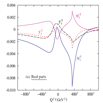
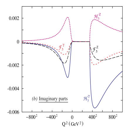
Figure 2: The $Q^{2}$ dependence of the four non-zero form-factors within the SM ($m_{t}=175\;{\rm GeV}$).

For a very large $Q^{2}$, all the SM fermions behave as if they are massless. Thus anomaly cancellation assures that asymptotically, all these form-factors must vanish. For relatively smaller values of $Q^{2}$, an analysis of eqns.(3efgi) shows that the relative contribution of each fermion loop grows with the fermion mass. The maximum contribution, thus, occurs for the heaviest fermion. On the other hand, it is clear that while ${\cal H}^{\gamma}_{3}$ and ${\cal F}_{5}^{\gamma}$ must vanish for $Q^{2}=0$, the other two (${\cal H}^{Z}_{3}$ and ${\cal F}_{5}^{Z}$) vanish as $Q^{2}\rightarrow m_{Z}^{2}$.

The imaginary parts of the four form-factors receive a contribution from a particular fermion loop only when the kinematics allows two of the fermions to be on-shell. This can happen for two different cases

1. if $Q^{2}>4m_{f}^{2}$ when the $s$-channel boson goes to a real pair of fermions. In Fig. 2($b$), this is evinced by the top thresholds.

2. for space-like momentum transfers with a real $Z$ in the final state such that $m_{Z}>2m_{f}$ where $m_{f}$ is the mass of the fermion in the loop. Clearly, the top-quark can never contribute to the imaginary parts for such “$t$-channel” (i.e. $Q^{2}<0$) processes. Since the light fermion contributions essentially cancel amongst each other, the magnitude of such imaginary parts are determined primarily by the $b$- and $\tau$-loops.

For the real parts, the situation is analogous, but slightly more complex. This part can be better in terms of a dispersion integral of the absorptive part [15]. The opening up of a channel now manifests itself as a kink, rather than a typical threshold jump. This, for example, is quite akin to the behaviour one sees in Higgs production through gluon-gluon fusion. For $Q^{2}<0$, one does not expect a threshold behaviour. That the form-factors have to fall off as $Q^{2}\to-\infty$ is obvious. The maximum shown by each curve can intuitively be understood in terms of ‘phase-space available’ as in a $t$-channel scattering.

5 TNGBVs within the MSSM

As we have already argued, to one-loop order, only the fermionic sector of a model may contribute to the form-factors under discussion. Going from the SM to the MSSM, the only augmentation of the fermionic spectrum is in the form of the chargino-neutralino sector. To recapitulate, the ($4\times 4$) mass matrix for the neutralinos is determined by four parameters, $M_{1,2}$, the soft supersymmetry breaking mass parameters for the $U(1)$ and $SU(2)$ gauginos, the Higgsino mass parameter $\mu$ and $\tan\beta$, the ratio of the vacuum expectation values of the two Higgs fields. The orthogonal matrix $N$ that diagonalizes this (real) symmetric mass matrix expresses the physical states in terms of the gauge eigenstates and thus enters the interaction vertices. On the other hand, the chargino mass matrix (determined by $M_{2}$, $\mu$ and $\tan\beta$) being real but nonsymmetric cannot be diagonalized by a single orthogonal matrix. Rather, one needs two such matrices $U$ and $V$ that left- and right-diagonalize it respectively. Writing the neutralino mass matrix in the $(\widetilde{B},\widetilde{W}_{3},\widetilde{H}_{1},\widetilde{H}_{2})$ basis and the chargino mass matrix in the $(\widetilde{W}^{+},\widetilde{H}^{+})$ basis, one can express [16] the relevant electromagnetic and weak currents as

$${\cal J}^{\mu}_{e.m}=\sum_{i}\overline{\tilde{\chi}_{i}^{+}}\;\gamma^{\mu}\tilde{\chi}_{i}^{+}$$ (3efgka)

and

$${\cal J}^{\mu}_{Z}=\sum_{i,j}\overline{\tilde{\chi}_{i}^{+}}\;\gamma^{\mu}\left(P_{L}\,O^{\prime L}_{ij}+P_{R}\,O^{\prime R}_{ij}\right)\tilde{\chi}_{j}^{+}+\sum_{\alpha,\beta}\,O^{\prime\prime}_{\alpha\beta}\,\overline{\tilde{\chi}^{0}_{\alpha}}\gamma^{\mu}\gamma_{5}\tilde{\chi}_{\beta}^{0}$$ (3efgkb)

where

$$\begin{array}[]{rcl}O^{\prime L}_{ij}&=&\displaystyle\sin^{2}\theta_{W}\,\delta_{ij}-\left({1\over 2}V_{i2}V_{j2}^{\star}+V_{i1}V_{j1}^{\star}\right)\\[6.45831pt] O^{\prime R}_{ij}&=&\displaystyle\sin^{2}\theta_{W}\,\delta_{ij}-\left({1\over 2}U_{i2}^{\star}U_{j2}\;+U_{i1}^{\star}U_{j1}\right)\\[6.45831pt] O^{\prime\prime}_{\alpha\beta}&=&\displaystyle{1\over 4}\left(N_{\alpha 3}N_{\beta 3}^{\star}-N_{\alpha 4}N_{\beta 4}^{\star}\right)\end{array}$$ (3efgkc)

Armed with the above, we can now calculate the MSSM contributions to the form-factors which were studied in the section 4 in the context of the SM.

5.1 Contribution to TNGBVs

As in the case of the SM, we start with the $Q^{2}$ dependence of the different form-factors. For this purpose, we choose a particular point in the MSSM parameter space namely $M_{2}=100\;{\rm GeV}$, $\mu=500\;{\rm GeV}$ and $\tan\beta=2$. For this set of parameters the chargino masses turn out to be $87.0\;{\rm GeV}$ and $515.1\;{\rm GeV}$, while the neutralino masses are $45.9\;{\rm GeV}$, $88.2\;{\rm GeV}$, $501.4\;{\rm GeV}$ and $517.7\;{\rm GeV}$. In each case, the gaugino component is the predominant one as far as the lighter eigenstates are concerned. While the charginos contribute to all of the TNGBVs, the neutralinos make their presence felt only in the $ZZZ$ vertex.

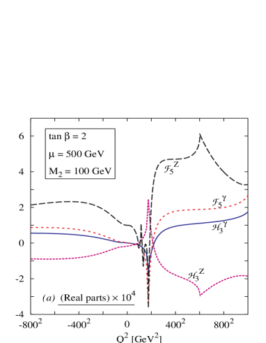
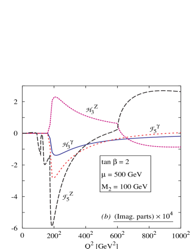
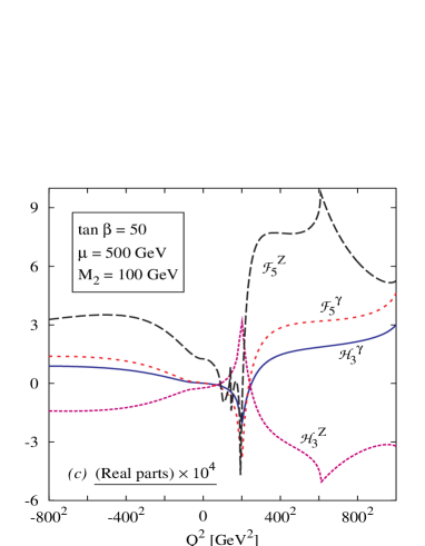
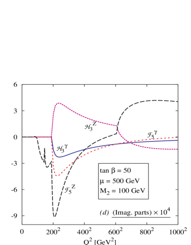
Figure 3: The $Q^{2}$ dependence of the purely supersymmetric contribution (within the MSSM) to the four non-zero form-factors.

As can be seen from Fig. 3, the $Q^{2}$ behaviour is quite analogous to that within the SM. The size of the contribution as well as the positions of the thresholds are of course different on account of the quantum numbers and the masses being different. For example, all of the form-factors exhibit the expected threshold behaviour at $Q^{2}=4M^{2}_{\tilde{\chi}^{+}_{1}}$. In addition, ${\cal F}_{5}^{Z}$ and ${\cal H}_{3}^{Z}$ show a second threshold kink at $Q^{2}=(M_{\tilde{\chi}^{+}_{1}}+M_{\tilde{\chi}^{+}_{2}})^{2}$. The other two form-factors do not exhibit corresponding kinks due to the presence of an off-shell photon which couples only to identical charginos. ${\cal F}_{5}^{Z}$ contains effects from neutralinos as well. However the charginos always dominate over the neutralinos except at the thresholds $2M_{\tilde{\chi}^{0}_{1}}$ and $M_{\tilde{\chi}^{0}_{1}}+M_{\tilde{\chi}^{0}_{2}}$. The fact, for our choice of referral parameters, of all the charginos and neutralinos having a mass larger than $m_{Z}/2$ has an obvious consequence. Referring back to the arguments in section 4, it is easy to see that the supersymmetric contribution to the imaginary parts of the form-factors vanishes identically for $Q^{2}<0$.

5.2 Dependence on the parameter space

To efficiently extract the parameter space dependence, it is useful to fix the momenta and so, in this section, we shall assume $Q^{2}=(500\;{\rm GeV})^{2}$—the popular choice for a linear collider center of mass energy—with the other two bosons being on mass-shell. We still are left with $\mu$, $M_{2}$ and $\tan\beta$. As Fig. 3 has already shown, the dependence on the last mentioned is quantitative rather than qualitative. Hence we shall keep it fixed at the intermediate value $\tan\beta=10$. In Fig. 4, we exhibit the $\mu$ dependence of $h_{3}^{\gamma}$ for two particular values of $M_{2}$.

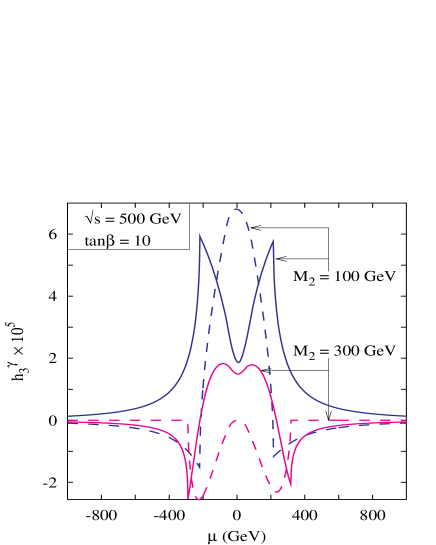
Figure 4: The dependence of the supersymmetric contribution to $h_{3}^{\gamma}$ on the Higgsino mass parameter $\mu$, for two particular values of $M_{2}$. The solid and dashed lines refer to the real and imaginary parts of the form-factor.

Let us concentrate first on the imaginary part for $M_{2}=300\;{\rm GeV}$. The two thresholds $\mu\approx-290\;{\rm GeV}$ and $\mu\approx 318\;{\rm GeV}$ represent the points beyond which the lighter chargino becomes heavier than $250\;{\rm GeV}$ and hence unable to contribute to the absorptive part. Understanding the behaviour for small $|\mu|$ takes a little more work. In this region, the lighter chargino is mainly a higgsino. Looking at eqns.(3efgh) and (3efgkc), it then becomes clear that the bulk of the contribution comes from terms proportional to the chargino mass. Consequently, a small $|\mu|$ implies a small imaginary part of the form-factor. For $M_{2}=100\;{\rm GeV}$, on the other hand, the gaugino state does contribute significantly. With the gaugino and higgsino gauge couplings being different, the interplay between the two is very crucial. This is what is responsible for the steep fall.

The same steep slope also implies that contour levels (for the imaginary part) in the $(\mu,M_{2})$ plane would be rapidly changing. This is reflected in the plots of Fig. 5, where we exhibit the behaviour of $h_{3}^{\gamma}$ and $h_{3}^{Z}$ as we vary either or both of $\mu$ and $M_{2}$ while maintaining $\tan\beta=10$.

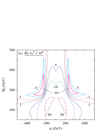
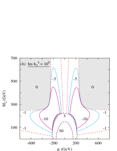
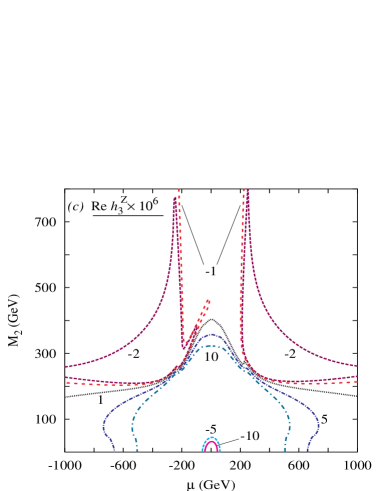
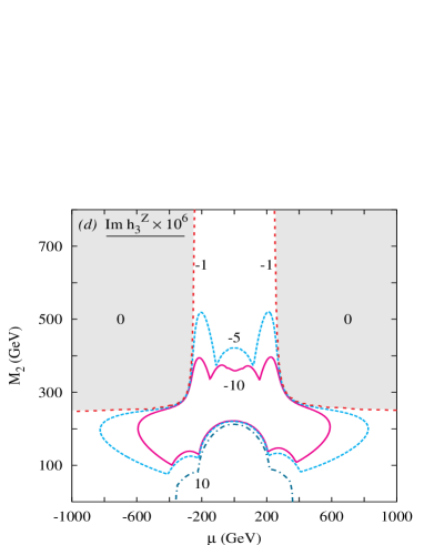
Figure 5: Contours for constant real and imaginary parts of the supersymmetric contribution to the form-factors ($\tan\beta=10$). In graphs (b) and (d), the shaded area denotes the parameter space where the imaginary parts of the form-factors are identically zero.

Let us consider the $\gamma\gamma Z$ vertex where at a time only one species of the charginos can flow inside the loop. Regarding the parameter space dependence, if one increases $M_{2}$ keeping $\mu$ and $\tan\beta$ fixed, then the heavier chargino ($\tilde{\chi}^{+}_{1}$) becomes more gaugino-like and correspondingly, the lighter one ($\tilde{\chi}^{+}_{2}$) becomes more higgsino-like. So as $M_{2}$ increases, the $Z\tilde{\chi}^{+}_{1}\tilde{\chi}^{-}_{1}$ coupling becomes stronger (remember the $Z$ couples to two $W^{\pm}$’s in the SM) and the $Z\tilde{\chi}^{+}_{2}\tilde{\chi}^{-}_{2}$ coupling becomes weaker. However, the diagram with $\tilde{\chi}^{+}_{1}$ flowing inside the loop suffers from large propagator suppressions in comparison with the other one containing $\tilde{\chi}^{+}_{2}$. Ultimately the magnitude of the total MSSM loop contribution to $h_{3}^{\gamma}$ decreases. If we choose to increase $\mu$ fixing $M_{2}$ and $\tan\beta$, $\tilde{\chi}^{+}_{1}$ becomes more higgsino-like. Here the diagram containing $\tilde{\chi}^{+}_{2}$ wins from both the strength of $Z\tilde{\chi}^{+}_{2}\tilde{\chi}^{-}_{2}$ coupling and the propagator suppressions. So in this case the total one-loop contribution falls off as well.

The parameter space dependence of other form-factors are more complicated as in those cases different types of charginos can co-exist inside the loop. However the basic reasoning is the same as above. As said earlier, the neutralinos contribute only to $f_{5}^{Z}$. The gaugino-like neutralinos can not contribute as there are no trilinear neutral gauge boson vertices at the tree level. Only the higgsino-like neutralinos contribute. However, as as the chargino contributions dominate over those from the neutralinos for most of the parameter space, we desist from discussing this issue any further.

6 Off-shell TNGBVs

Until now, we have dealt with the case wherein only one out of the three gauge bosons is off-shell. When more than one of them are off-shell, the form-factors are modified in two different ways. As the analysis of section 2 indicates, and as we shall shortly show, additional form-factors are possible. Apart from this, even the ones that we have considered are modified in a significant way. We examine the latter consequence first.

6.1 Modifications to ${\cal H}^{\gamma/Z}_{3}$ and ${\cal F}^{\gamma/Z}_{5}$

It is clear that now we can no longer talk in terms of $h^{\gamma/Z}_{3}$ etc. To take into account the explicit dependence on $p_{1}^{2}$ and $p_{3}^{2}$ as in eqns.(3b,3eb,3efb and 3efgb), it is imperative that we consider the full form-factors ${\cal H}^{\gamma/Z}_{3}$ and ${\cal F}^{\gamma/Z}_{5}$. Of course, over and above this explicit dependence on $p_{1,3}^{2}$, an additional dependence appears through the arguments of the Passarino-Veltman functions.

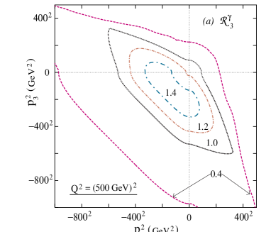
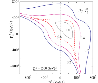
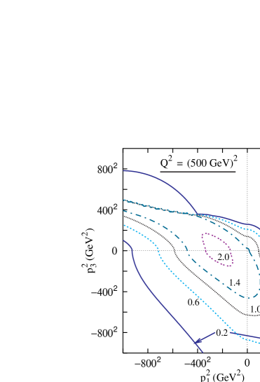
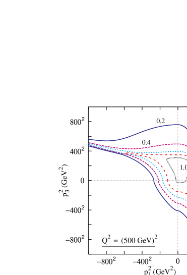
Figure 6: Constant ${\cal R}$ and ${\cal I}$ contours (see eqn.3efgkl) within the SM in the $(p_{1}^{2},p_{3}^{2})$ plane.

To quantify the changes wrought by the hitherto on-shell particles going off-shell, we define the ratios

$$\begin{array}[]{rcl}{\cal R}_{3}^{\gamma}&\equiv&\displaystyle\frac{[Re({\cal H}_{3}^{\gamma})]_{\rm off-shell}}{[Re({\cal H}_{3}^{\gamma})]_{\rm on-shell}}\\[12.91663pt] {\cal I}_{3}^{\gamma}&\equiv&\displaystyle\frac{[Im({\cal H}_{3}^{\gamma})]_{\rm off-shell}}{[Im({\cal H}_{3}^{\gamma})]_{\rm on-shell}}\end{array}$$ (3efgkl)

where the subscripts “on-shell” and “off-shell” are self-explanatory. Analogous definitions hold for ${\cal R}_{3}^{Z}$ and ${\cal I}_{3}^{Z}$. In Fig. 6 we present the contours for constant ${\cal R}_{3}^{\gamma/Z}$ and ${\cal I}_{3}^{\gamma/Z}$ in the $(p_{1}^{2},p_{3}^{2})$ plane for a fixed value $p_{2}^{2}=(500\;{\rm GeV})^{2}$.

As for the on-shell form-factors, it is interesting to consider the dependence on $p_{2}^{2}$. Naively, one would expect a behaviour broadly similar to that in Fig. 2. That this is indeed so can be seen by an examination of Fig. 7. At a first glance though, this assertion might seem unfounded since these figures do not seem to show all the features of Fig. 2, notably the kink. However, if one were to draw more contours for intermediate values, at the cost of cluttering the graph, such features spring out immediately.

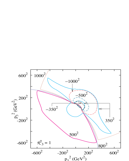
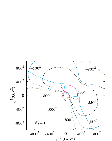
Figure 7: (a) Contours for ${\cal R}_{3}^{\gamma}=1$ in the $(p_{1}^{2},p_{3}^{2})$ plane for different values of $p_{2}^{2}$ (shown as legends). (b) Similar contours for ${\cal I}_{3}^{\gamma}=1$. All calculations are within the SM.

6.2 “Truly off-shell” form-factors

To identify all the possible additional form-factors that may arise when more than one of the bosons is off mass-shell, we revert back to eqn.(2) and restate it in a much more compact and simplified form. Gauge invariance implies that any term proportional to a photon momentum can be dropped without loss of generality. While this argument is not applicable for the $Z$, a very similar one holds. As long as the $Z$ couples only to light fermions ($m_{f}\ll\sqrt{s}$)—as is the case almost always—current conservation implies that terms proportional to the $Z$ momentum may be dropped as well. Within this approximation, then, either of $B_{2}$ and $\bar{B}_{2}$ are irrelevant. Restricting our analysis to one loop order further constrains ${\bar{B}_{3}}$ to be equal to $B_{3}$, vide eqn.(3efgi). Therefore, to this order,

$${\cal B}_{3}p_{1\mu}+\bar{\cal B}_{3}p_{2\mu}={\cal B}_{3}(p_{1}+p_{2})_{\mu}=-{\cal B}_{3}p_{3\mu}$$

Once again, this term may be dropped by virtue of current conservation. Thus, to one-loop, the generic TNGBV may be parametrized as

$$\Gamma_{\alpha\beta\mu}(p_{1},p_{2};p_{3})=\epsilon_{\alpha\beta\mu\eta}(B_{1}p_{1}^{\eta}-\bar{B}_{1}p_{2}^{\eta})$$ (3efgkm)

and, hence, there are at best two form-factors for each combination of the vector bosons. Let us now consider each in turn.

• $\gamma\gamma Z$ vertex

  Of the two form-factors in eqn. (3efgkm), the first, namely ${\cal B}_{1}$, is simply related to ${\cal H}_{3}^{\gamma}$ as defined for the on-shell case (see eqn. 3b). However, when the other gauge bosons are off-shell too, we have an additional form-factor, namely,

  $${\cal H}_{5}^{\gamma}=i\bar{{\cal B}_{1}}.$$ (3efgkn)

  While the variation of ${\cal H}_{5}^{\gamma}$ with each of the external momenta could be of interest, we restrict ourselves to the special situation wherein a comparison with ${\cal H}_{3}^{\gamma}$ is the easiest, namely $p_{2}^{2}=(500\;{\rm GeV})^{2}$. This particular value is of interest as it is widely considered to be the choice of center of mass energy for the first generation linear collider. In Fig. 8 we plot the variation of ${\cal H}_{5}^{\gamma}$ with $p_{1}^{2}$ for different values of $p_{3}^{2}$. As earlier, it is more instructive to concentrate on the imaginary part of the form-factor since the real part can then be obtained using a dispersion relation. Expectedly, in the imaginary part, we see a kink at $p_{1}^{2}=(2\,m_{t})^{2}$, with a corresponding dip in the real parts. Note that unlike in the case of Section 4, for a given fermion, the diagram may now be cut in more than one way and an imaginary contribution obtained. In Fig. 8, this feature manifests itself rather dramatically for $n=5$. Concentrating on the top-mediated diagram, a simple calculation shows that for $p_{1}^{2}\simeq-(900\;{\rm GeV})^{2}$, each of the three top-quarks could be on-shell. The kink thus corresponds to one particular cut ceding dominance to another.

  

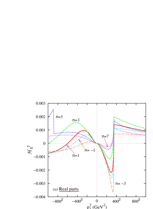
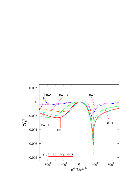
  Figure 8: The $Q^{2}$ dependence of the new non-zero form-factor ${\cal H}_{5}^{\gamma}$ within the SM for the off-shell $\gamma\gamma Z$ vertex for $p_{2}^{2}=(500\;{\rm GeV})^{2}$. $p_{3}^{2}=(n\;M_{Z})^{2}$ for positive n and $p_{3}^{2}=-\,(n\>M_{Z})^{2}$ when n is negative.

• $ZZ\gamma$ vertex

  Before manipulating eqn.(3efgkm), we reexpress it as

  $$\Gamma^{ZZ\gamma}_{\alpha\beta\mu}(p_{1},p_{2};p_{3})=\epsilon_{\alpha\beta\mu\eta}{1\over 2}\,\left[({\cal B}_{1}+\bar{\cal B}_{1})(p_{1}-p_{2})^{\eta}+({\cal B}_{1}-\bar{\cal B}_{1})(p_{1}+p_{2})^{\eta}\right]$$ (3efgko)

  On imposing gauge invariance (eqn.3d), this reduces to

  $$\Gamma^{ZZ\gamma}_{\alpha\beta\mu}(p_{1},p_{2};p_{3})=\epsilon_{\alpha\beta\mu\eta}{1\over 2}\,\left[{\cal B}_{3}p_{3}^{2}(p_{1}-p_{2})^{\eta}-({\cal B}_{1}-\bar{\cal B}_{1})p_{3}^{\eta}\right]$$

  These two form-factors have already been identified as ${\cal F}_{5}^{\gamma}$ and ${\cal H}_{3}^{Z}$ respectively. Thus, as expected, no additional form-factors appear even when we generalise to the case where all the gauge bosons are off-shell.

• $ZZZ$ vertex

  We could, once again, reexpress eqn.(3efgkm) as in the case for the $ZZ\gamma$ vertex. Note that while $({\cal B}_{1}+\bar{\cal B}_{1})$ corresponds to ${\cal F}_{5}^{Z}$, the orthogonal combination is a new form-factor in its own right. Thus, we may define ${\cal F}_{6}^{Z}$, via

  $${\cal F}_{6}^{Z}=i\frac{({\cal B}_{1}-\bar{\cal B}_{1})}{2}$$ (3efgkp)

  Obviously, ${\cal F}_{6}^{Z}$ vanishes identically for $p_{1}^{2}$ = $p_{3}^{2}$. And, given the symmetry of the problem, the iso-${\cal F}_{6}^{Z}$ contours in the $(p_{1}^{2},p_{3}^{2})$ plane are symmetric about this line. In Fig. 9, we display the momentum dependence of ${\cal F}_{6}^{Z}$ in a fashion similar to that for ${\cal H}_{5}^{\gamma}$. The behaviour of the curves can be understood in an analogous manner.

  

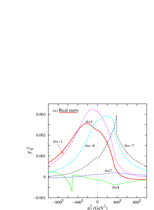
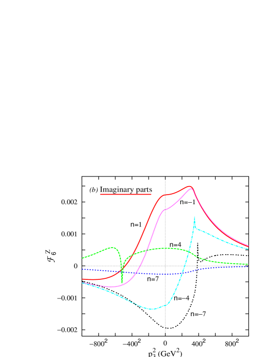
  Figure 9: The $Q^{2}$ dependence of the new non-zero form-factor ${\cal F}_{6}^{Z}$ within the SM for the off-shell $ZZZ$ vertex for $p_{2}^{2}=(500\;{\rm GeV})^{2}$. $p_{1}^{2}=(n\;M_{Z})^{2}$ for positive n and $p_{1}^{2}=-\,(n\>M_{Z})^{2}$ when n is negative.

7 Conclusions

In this paper we have considered the SM and MSSM contributions to trilinear neutral gauge boson vertices namely, $\gamma\gamma Z$, $ZZ\gamma$ and $ZZZ$ vertices. We discuss, in a systematic way, the tensor structure of the the three-point vertex. Starting with the most general CP conserving vertex, we first use Schouten’s identity to reduce the number of independent form-factors. Gauge invariance and Bose symmetry, whenever applicable, are used then to obtain the required structure. We have then provided explicit calculations for the form-factors [18, 11] relevant for these vertices at different limits, particularly when two out of these gauge bosons in a vertex are on-shell. We define total form-factors, ${\cal H}^{\gamma/Z}_{3,4}$ and ${\cal F}^{\gamma/Z}_{5}$, which are found to be more appropriate than the conventional (${h}^{\gamma/Z}_{3,4}$ and ${f}^{\gamma/Z}_{5}$) ones in discussions of off-shell behaviour.

At the one-loop level, only fermions contribute to these form-factors. Within the SM, these are the quarks and leptons, while, in the context of the MSSM, the charginos contribute too (neutralinos come into play only as far the $ZZZ$ vertex is concerned). We have provided explicit formulae for the generic form-factor as obtained from such loop diagrams. The calculations clearly demonstrate that ${\cal H}^{\gamma/Z}_{4}=0$ to this order, a conclusion in agreement with the observation made by Gounaris et al. [10].

We have studied the $Q^{2}$ dependence of these form-factors when two of the gauge bosons are on-shell for both SM and MSSM. Here we would like to emphasize the fact that these three point vertices can take part in $t$-channel processes and keeping this in mind we have presented values for both positive and negative $Q^{2}$. Cusps and peaks appear at the different thresholds defined by the masses of the internal fermions. The maximum magnitudes for the form-factors can be as high as $|Re[{\cal H}^{\gamma}_{3}]|\simeq 9\times 10^{-3}$ for SM at the top threshold, whereas for MSSM, the magnitude is smaller in most cases, the most promising one being $|Im[{\cal F}^{Z}_{5}]|\simeq 9\times 10^{-4}$ which depends on chargino and neutralino masses which, in turn, are parameter space dependent. One can expect this enhancement for ${\cal F}^{Z}_{5}$ due to almost degeneracy of the lightest chargino and next to lightest neutralino characteristic of this particular space and consequent opening of thresholds at similar $Q^{2}$ values.

These new physics effects are model dependent. So we have studied next the MSSM parameter space dependence of these form-factors. The contour plots of Fig. 5 should turn out to be useful to exclude certain regions of the parameter space if such new physics effects are estimated experimentally.

To get a better hold in determining these new physics effects, we have studied the effects on these form-factors when all the bosons are off-shell. It might turn out to be handy in identifying these effects as we can then have a better feeling of maximizing SUSY contributions playing with the off-shell vector bosons.

In short we have not only reviewed the SM contribution to triple neutral gauge boson vertices which will be relevant for a better understanding of the non-abelian structure of the SM, but also studied in detail the possible MSSM contributions to the same. These numerical estimations not only provide an independent verification of results provided by Ref. [10] but complement their results by providing the negative $Q^{2}$ values. Our study might also turn out to be useful to disentangle MSSM effects from the SM ones.

Acknowledgements
We would like to thank WHEPP5 organisers [19] where this work was initiated. S. Rakshit acknowledges partial support from the Council of Scientific and Industrial Research, India. Both S. Rakshit and S. Dutta would like to thank the Mehta Research Institute, Allahabad, for their hospitality while part of the work was being carried out.

References

-
[1]
The CDF Collaboration,
F. Abe et al., Phys. Rev. Lett. 74, 1936 (1995);
The D0 Collaboration, S. Abachi et al., Phys. Rev. D56, 6742 (1997). -
[2]
The ALEPH Collaboration, R. Barate et al.,
Phys. Lett. B469,
287 (1999); N. Konstantinidis, CERN-OPEN-99-275 (1999);
The DELPHI Collaboration, C. Matteuzzi et al., CERN-OPEN-2000-025; R. Jacobsson, in Lake Louise 1999, Electroweak Physics, p. 405;
The L3 Collaboration, M. Acciarri et al., Phys. Lett. B436, 187 (1998); Phys. Lett. B450, 281 (1999); M.A. Falagan, in Lake Louise 1999, Electroweak Physics, p. 371;
The OPAL Collaboration, G. Abbiendi et al., Phys. Lett. B476, 256 (2000). - [3] C. Ahn et al., SLAC-329 (1988); Proc. Workshops on Japan Linear Collider, KEK-90-2 (1990), ed. S. Kawabata, KEK Proc. 91-10 (1991), ed. S. Kawabata and KEK Proc. 92-13 (1992), ed. A. Miyamoto; P.M. Zerwas, DESY-93-112 (1993); Proc. of the Workshop on Collisions at 500 GeV: The Physics Potential, DESY-92-123A-B (1992) and DESY 93-123 (1993), ed. P.M. Zerwas; Proc. of the Workshop on Collisions at TeV Energies: The Physics Potential, Part D, DESY 96-123D (1996), ed. P.M. Zerwas; Proc. of the Workshop on Linear Colliders: Physics and Detector Studies, Part E, DESY 97-123E (1997), ed. R. Settles; E. Accomando et al., Phys. Rep. 299, 1 (1998).
- [4] R. Bossart et al., CERN-PS-99-005-LP (1999).
- [5] J. Alcaraz, M.A. Falagan and E. Sanchez, Phys. Rev. D61, 075006 (2000).
- [6] G. Gounaris et al., hep-ph/9601233; E.N. Argyres, A.B. Lahanas, C.G. Papadopoulos and V.C. Spanos, Phys. Lett. B383, 63 (1996); E.N. Argyres, G. Katsilieris, A.B. Lahanas, C.G. Papadopoulos and V.C. Spanos, Nucl. Phys. B391, 23 (1993); A. Arhrib, J.L. Kneur and G. Moultaka, Phys. Lett. B376, 127 (1996); The LEP-TGC Combination Group, LEPEWWG/TGC/2000-01 (March 2000), LEPEWWG/TGC/2000-02 (September 2000) and references therein.
- [7] U. Baur and E.L. Berger, Phys. Rev. D47, 4889 (1993); U. Baur, T. Han and J. Ohnemus, Phys. Rev. D57, 2823 (1998); U. Baur and D. Rainwater, Phys. Rev. D62, 113011 (2000) and references therein.
- [8] A. Barroso, F. Boudjema, J. Cole and N. Dombey, Z. Physik C28, 149 (1985).
- [9] G.J. Gounaris, J. Layssac and F.M. Renard, Phys. Rev. D61, 073013 (2000).
- [10] G.J. Gounaris, J. Layssac and F.M. Renard, Phys. Rev. D62, 073013 (2000).
- [11] K. Hagiwara, R.D. Peccei, D. Zeppenfeld and K. Hikasa, Nucl. Phys. B282, 253 (1987).
- [12] F.M. Renard, Nucl. Phys. B196, 93 (1982).
- [13] G. Passarino and M. Veltman, Nucl. Phys. B160, 151 (1979).
- [14] B. Mukhopadhyaya and A. Raychaudhuri, Phys. Rev. D39, 280 (1989); A. Raychaudhuri (unpublished); G.J. van Oldenborgh and J.A.M. Vermaseren, Z. Physik C46, 425 (1990); G.J. van Oldenborgh, Comput. Phys. Commun. 66, 1 (1991).
- [15] P. Poulose and S.D. Rindani, Pramana 51, 387 (1998); D. Choudhury and J. Ellis, Phys. Lett. B433, 102 (1998).
- [16] H.E. Haber and G.L. Kane, Phys. Rep. 117, 75 (1985).
- [17] G.J. Gounaris, J. Layssac and F.M. Renard, Phys. Rev. D62, 073012 (2000).
- [18] K.J.F. Gaemers and G.J. Gounaris, Z. Physik C1, 259 (1979).
- [19] B. Ananthanarayan et al., in Beyond the standard model: Working group report, Pramana 51, 305 (1998).