Abstract

We directly fit the QCD dimensional transmutation parameter, $\Lambda_{\overline{{\mathrm{MS}}}}$ , to experimental data on $\mbox{e}^{+}\mbox{e}^{-}\,\!$ jet observables, making use of next-to-leading order (NLO) perturbative calculations. In this procedure there is no need to mention, let alone to arbitrarily vary, the unphysical renormalisation scale ${\mu}$, and one avoids the spurious and meaningless “theoretical error” associated with standard $\alpha_{s}$ determinations. PETRA, SLD, and LEP data are considered in the analysis. An attempt is made to estimate the importance of uncalculated next-NLO and higher order perturbative corrections, and power corrections, by studying the scatter in the values of $\Lambda_{\overline{{\mathrm{MS}}}}$  obtained for different observables.

1 Introduction

The consistent extraction of the QCD coupling strength $\alpha_{s}$ from experimental data on a wide range of strong interaction processes has provided compelling evidence for Quantum Chromodynamics as the underlying theory of this sector of the Standard Model, for a recent comprehensive review see [1]. Notwithstanding attempts to exploit Lattice Gauge Theory calculations [2-4], the bulk of these determinations extract $\alpha_{s}$ by fitting the measured data to fixed-order perturbative predictions supplemented by computer-modelled hadronisation corrections. The asymptotic freedom of QCD leads one to hope that at sufficiently high energy scales (small enough values of the coupling) these determinations will be reasonably accurate. In this paper we shall be concerned with jet observables such as jet rates, thrust distributions,…, studied in $\mbox{e}^{+}\mbox{e}^{-}\,\!$ collisions. For these observables next-to-leading order (NLO) perturbative corrections have been calculated [5-8], and non-perturbative hadronisation (power) corrections can be modelled using a variety of computer Monte Carlo techniques [8, 9]. A difficulty with fixed-order renormalisation group (RG)-improved perturbation theory is that NLO predictions depend on the dimensionful renormalisation scale $\mu$ which arises in removing ultraviolet divergences from the calculation. Usually one chooses $\mu$ proportional to $Q$ the physical energy scale of the process, for instance the c.m. energy in $\mbox{e}^{+}\mbox{e}^{-}\,\!$ collisions, so that ${\mu}=xQ$, with $x$ an unspecified dimensionless constant. This is then varied over some range around ${\mu}=Q$, $x=1$, the so-called “physical scale”, say between ${\mu}=10Q$ and ${\mu}=0.1Q$. The resulting fits to data of ${\alpha}_{s}(xQ)$ are then customarily converted to ${\alpha}_{s}(M_{Z})$ using the two-loop evolution of the coupling to yield a central value based on $x=1$, and a “theoretical error bar” based on the variation between $x=10$ and $x=0.1$. Unfortunately, the range of $x$ to be considered is completely ad hoc, and there is no reason why the central values obtained should reflect the actual value of ${\alpha}_{s}(M_{Z})$. According to [1] this arbitrariness leads to “infinite discomfort in finite order”. The cure for this discomfort is to recognise that the dimensionful scale $\mu$ has no physical relevance whatsoever. The fact that fixed-order RG-improved perturbative predictions depend on it is a result of the standard way in which RG-improvement is carried out [10, 11], with the perturbation series being truncated at NLO, and a choice of scale which is $Q$-dependent. One should rather keep $\mu$ independent of $Q$. The renormalisation scheme-dependent coupling ${\alpha}_{s}({\mu})$ then has no dependence on $Q$, the $Q$-dependence of the observable coming entirely from the perturbative coefficients which contain “unphysical” $\mu$-dependent logarithms and “physical” $Q$-dependent ultraviolet (UV) logarithms. Fixed-order truncation of the perturbation series is no longer adequate, in particular such truncations with $\mu$ independent of $Q$ do not satisfy asymptotic freedom. The RG self-consistency of perturbation theory allows one to identify an infinite subset of RG-predictable logarithms at any given order of Feynman diagram calculation. If these are resummed to all-orders the “unphysical” $\mu$-dependent logarithms contained in ${\alpha}_{s}(\mu)$ cancel against those contained in the perturbative coefficients, and one obtains a $\mu$-independent result, which correctly builds the leading $Q$-dependence of the observable. This procedure has been termed “Complete Renormalisation Group Improvement” (CORGI) [10, 11], and it has been shown how to extend the argument to problems involving factorisation scales in addition to renormalisation scales [11]. At NLO this approach yields exactly the same result as the Effective Charge approach of Grunberg [12, 13], which corresponds to choosing $\mu$ with standard RG-improvement in such a way that all the “physical” UV logarithms of $Q$ are resummed. In general with the standard RG-improvement an infinite subset of these logarithms is omitted, with the result that one obtains ${\mu}$-dependent results, and does not reproduce the correct physical leading $Q$-dependence of the observable.

In fact it is possible to motivate this approach more straightforwardly by showing how QCD observables may be directly related to the dimensional transmutation parameter of the theory. In Section 2 we shall show how the dimensional transmutation parameter arises on the grounds of generalised dimensional analysis, modifying the analysis of [14]. The form of this relation at the NLO level is then completely equivalent to the CORGI approach outlined above. The advantage of this derivation is that mention of the renormalisation scale $\mu$ and the renormalised coupling ${\alpha}_{s}({\mu})$ can be essentially avoided, and the physical irrelevance of these quantities is manifest. In contrast the fundamental importance of the parameter $\Lambda$ is stressed. In Section 3 we shall define the QCD $\mbox{e}^{+}\mbox{e}^{-}\,\!$ jet observables with which we shall be concerned. Section 4 contains direct plots of $\Lambda_{\overline{{\mathrm{MS}}}}$  obtained bin-by-bin in jet resolution criterion, thrust,…,etc., from hadronisation corrected data, using the direct relation between $\Lambda_{\overline{{\mathrm{MS}}}}$  and the data. We attempt to estimate the uncertainty in $\Lambda_{\overline{{\mathrm{MS}}}}$  due to uncalculated NNLO and higher-order corrections, and possible power corrections, by looking at the scatter in the extracted values between different observables. In Section 5 we study the dependence of the thrust distribution on the c.m. energy $Q$ using data spanning the PETRA-LEP 1-LEP 2 energy range, and we perform joint fits for NNLO perturbative corrections and power corrections. Section 6 contains a discussion and our Conclusions.

2 Direct Relation between $\boldsymbol{\Lambda}$ and QCD Observables

In this section we shall derive from basic considerations of generalised dimensional analysis how the dimensional transmutation parameter ${\Lambda}$ arises, and how it may be directly related to the QCD observable. The derivation owes much to the discussion of [14] and closely follows that of [15]. We suppose that we have a dimensionless generic QCD observable ${\mathcal{R}}(Q)$, dependent on the single dimensionful (energy) scale $Q$. Quark masses will be taken to be zero throughout our discussion, the extension to the massive case has been considered in [16]. Since ${\mathcal{R}}(Q)$ is dimensionless, dimensional analysis clearly demands that

$${\mathcal{R}}(Q)={\Phi}\left(\frac{\Lambda}{Q}\right)\;,$$ (1)

where $\Lambda$ is a dimensionful scale , which will turn out to be related to the dimensional transmutation parameter. There is an extra trivial possibility that ${\mathcal{R}}(Q)=C$, where $C$ is a dimensionless constant. That is, there is no energy dependence. This trivial $Q$-dependence would be the case if the bare coupling of QCD was finite, since the QCD Lagrangian (with massless quarks) contains no massive parameters. Of course, in fact, the bare coupling is infinite, and an infinite renormalisation must be performed, leading to a functional relation as in Eq.(1). An obvious proposal is to invert Eq.(1) to obtain

$$\frac{\Lambda}{Q}={\Phi}^{-1}({\mathcal{R}}(Q)),$$ (2)

where ${\Phi}^{-1}$ is the inverse function. This is indeed the basic motivation for Grunberg’s method of Effective Charges [13]. We shall obtain the form of ${\Phi}^{-1}$ by starting from the form of the derivative of ${\mathcal{R}}(Q)$ with respect to $Q$, imposed by dimensional analysis. We must clearly have,

$$\frac{\mathrm{d}{\mathcal{R}}(Q)}{\mathrm{d}Q}=\frac{B({\mathcal{R}}(Q))}{Q}\;,$$ (3)

where $B({\mathcal{R}}(Q))$ is a dimensionless function of $\mathcal{R}$ . This can be rearranged to obtain,

$$\frac{\mathrm{d}{\mathcal{R}}(Q)}{\mathrm{d}\,{\ln}Q}=B({\mathcal{R}}(Q))\;.$$ (4)

This is a separable first-order differential equation. In order to solve it we will need to impose a boundary condition, and to know something of the behaviour of $B({\mathcal{R}})$. We shall assume that ${\mathcal{R}}$ has the perturbative expansion,

$${\mathcal{R}}=a\left(1+{\sum_{n>0}}{r_{n}}{a}^{n}\right)\;,$$ (5)

where $a{\equiv}{\alpha_{s}({\mu})}/{\pi}$ is the RG-improved coupling. The form of expansion in Eq.(5) can always be arranged by suitably scaling the observable and raising to an appropriate power. The required boundary condition will be given by asymptotic freedom, that is ${\mathcal{R}}({\infty})=0$. Integrating Eq.(4) one then obtains

$${\ln}\frac{Q}{{\Lambda}_{\mathcal{R}}}={\int_{0}^{{\mathcal{R}}(Q)}}\frac{dx}{B(x)}\;+{\kappa}\;.$$ (6)

The constant of integration has been split into ${\ln}{\Lambda}_{\mathcal{R}}+{\kappa}$, where ${\Lambda}_{\mathcal{R}}$ is a finite dimensionful scale specific to the observable ${\mathcal{R}}$, and ${\kappa}$ is a universal infinite constant needed to implement ${\mathcal{R}}({\infty})=0$. To determine $\kappa$ we need to know the behaviour of $B(x)$ around $x=0$. Returning to the perturbative series of Eq.(5) we note that the coupling $a$ satisfies the beta-function equation,

$${\mu}\frac{\partial a}{\partial{\mu}}={\beta}(a)=-b{a}^{2}\left(1+ca+{\sum_{n>1}}{c_{n}}{a}^{n}\right)\;,$$ (7)

where $b=(33-2{N_{f}})/6$ , and $c=(153-19{N_{f}})/12b$, are the first two coefficients of the beta-function for SU(3) QCD with $N_{f}$ active (massless) flavours of quark. They are universal, whereas the subsequent coefficients $c_{i},(i>1)$ are scheme-dependent. In fact, as shown by Stevenson [17], the non-universal beta-function coefficients can be used to label the renormalisation scheme (RS), together with the renormalisation scale. If we set ${\mu}=Q$ in Eq.(5), and differentiate with respect to ${\ln}Q$ term-by-term using the beta-function equation (7), we can obtain $B({\mathcal{R}}(a))$ as a power series in $a$, finally if we invert the series ${\mathcal{R}}(a)$ in Eq.(5) to obtain $a({\mathcal{R}})$ as a power series in ${\mathcal{R}}$, we can obtain $B({\mathcal{R}})$ as a power series in ${\mathcal{R}}$ . One finally finds for the series expansion of $B(x)$ around $x=0$,

$$B(x)=-b{x}^{2}\left(1+c{x}+{\sum_{n>1}}{\rho}_{n}{x}^{n}\right)\;.$$ (8)

The first two coefficients $b$, $c$, are the universal beta-function coefficients. The higher terms ${\rho}_{i},(i>1)$ are renormalisation scheme (RS)-invariant, and $Q$-independent, combinations of the ${r_{i}}$ and ${c_{i}}$. The first two are [13, 15, 17]

$${\rho}_{2} = {c_{2}}+{r_{2}}-{r_{1}}{c}-{r}_{1}^{2}$$

$${\rho}_{3} = {c_{3}}+2{r_{3}}-4{r_{1}}{r_{2}}-2{r_{1}}{\rho}_{2}-{r}_{1}^{2}c+2{r}_{1}^{3}\;.$$ (9)

Knowledge of ${\rho}_{n}$ requires a complete ${\rm{N}}^{n}$LO perturbative calculation, that is a calculation of the $r_{i}$ for $i=1,2,{\ldots},n$ and the ${c_{i}}$ for $i=2,3,{\ldots},n$ , in some renormalisation scheme, for instance $\overline{{\mathrm{MS}}}$. The fact that Eq.(8) has the same form as the beta-function equation (7) follows from the fact that there exists an RS in which ${\mathcal{R}}=a$, i.e. ${r_{i}}=0,i>0$, and in this scheme the non-universal beta-function coefficients are ${c_{i}}={\rho}_{i}$, $i>1$. The existence of this Effective Charge scheme [13] is underwritten by the algebraic steps above from which (8) can be directly derived. Armed with knowledge of the form of $B(x)$ around $x=0$ we see that the infinite constant of integration ${\kappa}$ will be of the form

$${\kappa}=-{\int_{0}^{C}}\frac{dx}{K(x)},$$ (10)

where $K(x)$ must be such that the singularity of $1/B(x)$ at $x=0$ in (6) is cancelled. This implies from (8) that

$$K(x)=-b{x}^{2}(1+cx+{\Delta}(x)),$$ (11)

where ${\Delta}(x)$ is only constrained by the requirement that ${\Delta}(x)/{x^{2}}$ is finite as $x{\rightarrow}0$. Different choices of the upper limit of integration, $C$, and the function ${\Delta}(x)$, can be absorbed into the dimensionful constant ${\Lambda}_{\mathcal{R}}$. Convenient choices are $C={\infty}$ and ${\Delta}(x)=0$. With these choices (6) can be re-written as,

$$b{\ln}\frac{Q}{{\Lambda}_{\mathcal{R}}}={\int_{{\mathcal{R}}(Q)}^{\infty}}\frac{dx}{{x^{2}}(1+cx)}+{\int_{0}^{{\mathcal{R}}(Q)}}{dx}\left[\frac{b}{{B}(x)}+\frac{1}{{x^{2}}(1+cx)}\right]\;.$$ (12)

The first integral on the r.h.s. of (12) gives

$$F({\mathcal{R}}){\equiv}\frac{1}{{\mathcal{R}}}+c{\ln}\left[\frac{c{\mathcal{R}}}{1+c{\mathcal{R}}}\right]\;.$$ (13)

Denoting the second integral by $G({\mathcal{R}})$ we have

$$b{\ln}\frac{Q}{{\Lambda}_{\mathcal{R}}}=F({\mathcal{R}})+G({\mathcal{R}})\;.$$ (14)

The desired inverse function ${\Phi}^{-1}$ of (2) can then be obtained by exponentiating (14), which gives

$${\mathcal{F}}({\mathcal{R}}(Q)){\mathcal{G}}({\mathcal{R}}(Q))=\frac{{\Lambda}_{\mathcal{R}}}{Q}\;$$ (15)

where ${\mathcal{F}}$ is the universal function

$${\mathcal{F}}({\mathcal{R}}){\equiv}{e}^{-F({\mathcal{R}})/b}={e}^{-1/b{\mathcal{R}}}{(1+1/c{\mathcal{R}})}^{c/b}\;,$$ (16)

and

$${\mathcal{G}}({\mathcal{R}}){\equiv}{e}^{-G({\mathcal{R}})/b}={\exp}\left[-{\int_{0}^{{\mathcal{R}}(Q)}}{dx}\left(\frac{1}{B(x)}+\frac{1}{b{x}^{2}(1+cx)}\right)\right]\;.$$ (17)

If only a NLO perturbative calculation has been completed then our state of knowledge of $B(x)$ is $B(x)=-b{x}^{2}(1+cx)$ since the NNLO and higher RS invariants ${\rho}_{2},{\rho}_{3},{\ldots}$ of (8) will be unknown. From (17) we then have ${\mathcal{G}}({\mathcal{R}})=1$. We finally need to relate the observable-dependent constant of integration ${\Lambda}_{\mathcal{R}}$ which arose on integrating (4), to the universal dimensional transmutation constant which depends only on the subtraction procedure used to remove the ultraviolet divergences, $\Lambda_{\overline{{\mathrm{MS}}}}$  for instance. Fortunately it turns out that they can be related exactly given only a one-loop (NLO) perturbative calculation of the observable. To see this we begin by noting that on rearranging (14) and taking the limit as $Q{\rightarrow}{\infty}$ , we obtain an operational definition of ${\Lambda}_{\mathcal{R}}$,

$${\Lambda}_{\mathcal{R}}={\lim_{Q\rightarrow{\infty}}}Q{\exp}(-F({\mathcal{R}}(Q))/b)\;.$$ (18)

We have used the fact that $G(0)=0$ together with asymptotic freedom. If we denote by $a(Q)$ the $\overline{{\mathrm{MS}}}$ coupling with ${\mu}=Q$ we see that it will satisfy the beta-function equation (7), of the same form as (4) for ${\mathcal{R}}$, with ${\beta}_{\overline{{\mathrm{MS}}}}(a)$ replacing $B({\mathcal{R}})$. This may be integrated following the same steps as above. The constant of integration ${\Lambda}_{\mathcal{R}}$ will be replaced by ${\tilde{\Lambda}_{\overline{{\mathrm{MS}}}}}$, and the coefficients ${\rho}_{i}$ by the $\overline{{\mathrm{MS}}}$ beta-function coefficients ${c}_{i}^{\overline{{\mathrm{MS}}}}$. Again choosing $C={\infty}$ and ${\Delta}(x)=0$, we arrive at

$${\tilde{\Lambda}}_{\overline{{\mathrm{MS}}}}={\lim_{Q\rightarrow{\infty}}}Q{\exp}(-F(a(Q))/b)\;.$$ (19)

From the perturbative expansion of ${\mathcal{R}}$ in (5) we will have

$${\mathcal{R}}(Q)={a(Q)}+{r}{(a(Q))}^{2}+{\ldots}\;,$$ (20)

where we have defined for convenience ${r}{\equiv}{r}_{1}^{\overline{{\mathrm{MS}}}}({\mu}=Q)$, as the notation suggests $r$ is Q-independent. It is then straightforward to show that as $Q{\rightarrow}{\infty}$

$$F({\mathcal{R}}){\approx}F(a)-{r}+{\ldots}\;,$$ (21)

where the ellipsis denotes terms which vanish as ${Q}{\rightarrow}{\infty}$. Inserting this result into (18), and comparing with (19), one finally finds

$${\Lambda}_{\mathcal{R}}={e}^{r/b}{\tilde{\Lambda}}_{\overline{{\mathrm{MS}}}}\;,$$ (22)

for the promised exact relation between the observable-dependent and universal ${\Lambda}$’s. The tilde over ${\Lambda}$ is to draw attention to the fact that the above choice of infinite integration constant ${\kappa}$ does not accord with the standard choice [18], which is based on an expansion of $a$ in inverse powers of ${\ln}({\mu}^{2}/{\Lambda}^{2})$. This definition corresponds to translating ${\kappa}$ by the finite shift $c\>\!{\ln}({b}/{2c})$, so that the standard $\Lambda_{\overline{{\mathrm{MS}}}}$  is related to ${\tilde{\Lambda}}_{\overline{{\mathrm{MS}}}}$ by

$${\tilde{\Lambda}}_{\overline{{\mathrm{MS}}}}={\left(\frac{2c}{b}\right)}^{-c/b}{\Lambda}_{\overline{{\mathrm{MS}}}}\;.$$ (23)

Finally assembling all this we arrive at the desired relation between the universal dimensional transmutation parameter $\Lambda_{\overline{{\mathrm{MS}}}}$  and the QCD observable ${\mathcal{R}}$,

$$\Lambda_{\overline{{\mathrm{MS}}}}\,=Q{\mathcal{F}}({\mathcal{R}}(Q)){\mathcal{G}}({\mathcal{R}}(Q)){e}^{-r/b}{(2c/b)}^{c/b}\;.$$ (24)

Notice that all dependence on the subtraction convention chosen to remove ultraviolet divergences resides in the single factor ${e}^{-r/b}$, the remainder of the expression being independent of this choice. This is equivalent to the observation of Celmaster and Gonsalves [19] that ${\Lambda}$’s with different subtraction conventions can be exactly related given a one-loop (NLO) calculation.
As noted above if only a NLO calculation has been performed then the state of our knowledge of the function $B({\mathcal{R}})$ in (4) is $B({\mathcal{R}})=-b{\mathcal{R}}^{2}(1+c{\mathcal{R}})$, and then from (17) ${\mathcal{G}}({\mathcal{R}})=1$. So at NLO the best we can do in extracting $\Lambda_{\overline{{\mathrm{MS}}}}$  from the data is

$$\Lambda_{\overline{{\mathrm{MS}}}}\,=Q{\mathcal{F}}({\mathcal{R}}(Q)){e}^{-r/b}{(2c/b)}^{c/b}\;.$$ (25)

If two-loop (NNLO) and higher-order perturbative calculations are available then ${\mathcal{G}}({\mathcal{R}})$ will differ from unity by calculable corrections. One can expand ${\mathcal{G}}({\mathcal{R}})$ as a power series in $\mathcal{R}$,

$${\mathcal{G}}({\mathcal{R}})=1-\frac{{\rho}_{2}}{b}{\mathcal{R}}+O({\mathcal{R}}^{2})+{\ldots}\;,$$ (26)

where ${\rho}_{2}$ is the NNLO RS-invariant defined in (9). Alternatively $G({\mathcal{R}})$ can be expanded in the exponent as a power series in ${\mathcal{R}}$ by expanding the integrand in (17), to give

$${\mathcal{G}}({\mathcal{R}})={\exp}[(-{\rho}_{2}{\mathcal{R}}+O({\mathcal{R}}^{2})+{\ldots})/b]\;.$$ (27)

One could also evaluate the integral in (17) numerically with $B(x)$ truncated, so that at NNLO for instance $B(x)=-b{x^{2}}(1+cx+{\rho}_{2}{x^{2}})$.

Focussing now on the NLO case where ${\mathcal{G}}=1$ we note that (25) can be inverted to give

$${\mathcal{R}}(Q) = -\frac{1}{c[1+W(z(Q))]}$$

$$z(Q) {\equiv} -\frac{1}{e}{\left(\frac{Q}{{\Lambda}_{\mathcal{R}}}\right)}^{-b/c}\;,$$ (28)

where $W$ is the Lambert $W$-function [21, 22] defined implicitly by the equation $W(z){\exp}(W(z))=z$. To be consistent with asymptotic freedom it is actually the $W_{-1}$ branch of the function which is required [22]. Eq.(28) is equivalent to the two-loop $\overline{{\mathrm{MS}}}$ coupling with scale ${\mu}={e}^{-r/b}Q$, and in this scheme ${r_{1}}=0$. This scheme is sometimes referred to as the “Fastest Apparent Convergence” (FAC) scheme [17], and is equivalent to Grunberg’s Effective Charge approach at NLO [12, 13]. Crucially, we have derived (28) without having to argue for a specific choice of scale. Starting from the form of $Q$-dependence of ${\mathcal{R}}$ implied by dimensional analysis in (3), we simply solved this differential equation applying asymptotic freedom as a boundary condition. To define the required infinite constant of integration we needed to know the series expansion of $B(x)$ around $x=0$, Eq.(8), whose form is completely scheme-independent, and we thus arrived at Eq.(14). The constant of integration ${\Lambda}_{\mathcal{R}}$ could then be exactly related to the universal dimensional transmutation parameter $\Lambda_{\overline{{\mathrm{MS}}}}$  associated with use of $\overline{{\mathrm{MS}}}$ subtraction to remove ultraviolet divergences, given a NLO calculation of $r$, as in Eq.(22). In all of this the renormalised coupling $a$ only ever appeared in intermediate steps, playing, as neatly expressed in [14], “the role of a conjuror’s handkerchief- now you see it, now you don’t!”. This, of course, begs the question as to what is special about the Effective Charge (FAC) scheme, and why other choices of scale ${\mu}$ do not provide equally valid predictions for ${\mathcal{R}}$. The key is to identify the way in which the $Q$-dependence of ${\mathcal{R}}(Q)$ arises. In the construction above it is built automatically by integration of (3), but how does it arise from the perturbation series in Eq.(5) ? The crucial observation is that the perturbative coefficients ${r_{i}}$ contain ultraviolet logarithms of $Q$. To see this we can rearrange Eq.(22) to obtain

$$r=b{\ln}\frac{Q}{{\tilde{\Lambda}}_{\overline{{\mathrm{MS}}}}}-b{\ln}\frac{Q}{{\Lambda}_{\mathcal{R}}}\;,$$ (29)

or for a general choice of ($\overline{{\mathrm{MS}}}$) scale $\mu$ ,

$${r_{1}}({\mu})=b{\ln}\frac{\mu}{{\tilde{\Lambda}}_{\overline{{\mathrm{MS}}}}}-b{\ln}\frac{Q}{{\Lambda}_{\mathcal{R}}}\;.$$ (30)

Thus $r_{1}$ is a difference of a scheme-dependent logarithm involving $\mu$ and a “physical” scheme-independent ultraviolet logarithm involving $Q$. In RG-improvement as customarily applied one chooses ${\mu}=xQ$, and so the renormalised coupling $a(xQ)$ is $Q$-dependent. The perturbative coefficients ${r_{i}}({\mu}=Q)$, however, are $Q$-independent. The consistency of perturbation theory means that higher coefficients $r_{i}$ are ${i}^{\rm{th}}$-order polynomials in $r_{1}$ with $Q$-independent, but scheme-dependent coefficients [10, 11, 17]. Rearrangement of Eq.(9), for instance, gives

$${r_{2}} = {r}_{1}^{2}+{r}_{1}c+({\rho}_{2}-{c_{2}})$$

$${r_{3}} = {r}_{1}^{3}+\frac{5}{2}c{r}_{1}^{2}+(3{\rho_{2}}-2{c_{2}}){r_{1}}+(\frac{{\rho}_{3}}{2}-\frac{c_{3}}{2})\;.$$ (31)

From Eq.(30) we see that ${r_{1}}({\mu}=xQ)$ is $Q$-independent, and it follows from (31) that ${r_{2}},{r_{3}},{\ldots}$, are therefore $Q$-independent too. Thus the $Q$-dependence comes entirely from the renormalised coupling, and is hence dependent on the unphysical renormalisation scheme parameter $x$. In contrast the idea of Complete RG-improvement (CORGI) [10, 11] is to keep $\mu$ strictly independent of $Q$. In which case the $Q$-dependence is built entirely by the ultraviolet logarithms of $Q$ contained in the perturbative coefficients. Standard NLO fixed-order perturbation theory is then manifestly inapplicable, since one has

$${\mathcal{R}}_{NLO}=a({\mu})+\left(b{\ln}\frac{{\mu}}{{\tilde{\Lambda}}_{\overline{{\mathrm{MS}}}}}-b{\ln}\frac{Q}{{\Lambda}_{\mathcal{R}}}\right){(a({\mu}))}^{2}\;.$$ (32)

With $\mu$ constant, asymptotic freedom only arises if all the RG-predictable UV logarithms are resummed to all-orders. Given only a NLO calculation the RS-invariants ${\rho}_{i},(i>1)$ are unknown, and so the resummation of the RG-predictable UV logarithms corresponds to setting the ${\rho}_{i}$ to zero in Eq.(31). If we further set $c=0$ and ${c_{i}}=0,(i>1)$ , to simplify the analysis then the all-orders sum of RG-predictable terms reduces to a geometric series,

$${\mathcal{R}}=a({\mu})\left(1+{\sum_{n>0}}{(a({\mu}){r}_{1}({\mu}))}^{n}\right)\;.$$ (33)

With these simplifications we will have $a({\mu})=1/b{\ln}({\mu}/{\tilde{\Lambda}}_{\overline{{\mathrm{MS}}}})$, and using Eq.(30) and summing the geometric series one obtains,

$${\mathcal{R}}(Q)=a({\mu})/\left[1-\left(b{\ln}\frac{{\mu}}{{\tilde{\Lambda}}_{\overline{{\mathrm{MS}}}}}-b{\ln}\frac{Q}{{\Lambda}_{\mathcal{R}}}\right)a({\mu})\right]=1/b{\ln}(Q/{\Lambda}_{\mathcal{R}})\;,$$ (34)

in which the unphysical $\mu$-dependence has cancelled between $a({\mu})$ and the $\mu$-dependent logarithms contained in ${r}_{1}({\mu})$. In the realistic case with nonzero $c$ and $c_{i}$ the simple logarithm of $Q/{\Lambda}_{\mathcal{R}}$ is replaced by the Lambert $W$-function of Eq.(28). The key point is that the all-orders CORGI improvement can be carried out with any choice of $\mu$ to yield a $\mu$-independent result. One has therefore directly traded unphysical $\mu$-dependence for the physical $Q$-dependence.

To further emphasise the connection of the suggested direct extraction of $\Lambda_{\overline{{\mathrm{MS}}}}$  with the standard approach we can consider the following result for ${\Lambda}_{\overline{MS}}({r_{1}},{\mathcal{R}})$, which we define to be the value of $\Lambda_{\overline{{\mathrm{MS}}}}$  obtained by fitting a NLO perturbative calculation in a scheme corresponding to the NLO coefficient $r_{1}$, to the data ${\mathcal{R}}$ . Notice that $r_{1}$ completely labels the scheme at NLO. We can directly convert $r_{1}$ into the $\overline{{\mathrm{MS}}}$ scale $\mu$ since from (29) and (30) we have

$${r_{1}}=r+b{\ln}\frac{{\mu}}{Q}\;.$$ (35)

It is then straightforward to derive the result [15]

$${\Lambda_{\overline{{\mathrm{MS}}}}\,({r_{1}},{\mathcal{R}})=\frac{{\exp}[f({r_{1}},{\mathcal{R}})/b]}{{\mathcal{G}}({\mathcal{R}})}\;\Lambda_{\overline{{\mathrm{MS}}}}\,}\;,$$ (36)

where $f({r_{1}},{\mathcal{R}})$ is given by

$$f({r_{1}},{\mathcal{R}}){\equiv}F({\mathcal{R}})-F\left(\frac{-1+\sqrt{1+4{r_{1}}{\mathcal{R}}}}{2{r_{1}}}\right)+{r_{1}}\;.$$ (37)

In the CORGI approach ${r_{1}}=0$ and we have $f(0,{\mathcal{R}})=0$, so that the value of $\Lambda_{\overline{{\mathrm{MS}}}}$  obtained is $\Lambda_{\overline{{\mathrm{MS}}}}\,/{\mathcal{G}}({\mathcal{R}})$, as expected comparing (24) and (25). Thus to the extent that ${\mathcal{G}}({\mathcal{R}}){\approx}1$ we obtain the actual value of $\Lambda_{\overline{{\mathrm{MS}}}}$ . As we have argued the estimate ${\mathcal{G}}({\mathcal{R}}){\approx}1$ is the best we can do given only a NLO calculation since we are in complete ignorance of the deviations of ${\mathcal{G}}$ from unity, which will depend on the NNLO RS-invariant ${\rho}_{2}$ of Eq.(9). Another way of saying this is that at asymptotic values of $Q$ Eq.(25) will hold, and that the deviation of ${\mathcal{G}}({\mathcal{R}})$ from unity provides an operational definition of how far from asymptotia we are, at $Q={M_{Z}}$, say. The scatter of the $\Lambda_{\overline{{\mathrm{MS}}}}$  values for different observables obtained from Eq.(25) thus provides unambiguous information about the size of sub-asymptotic effects (uncalculated NNLO and higher perturbative corrections and power corrections). Variation of the renormalisation scale taking ${\mu}=xQ$ with the “physical scale” $x=1$ giving a central value merely serves to confuse matters. For instance taking $r=10$ and ${\mathcal{R}}=0.05$, values typical of jet observables at $Q={M_{Z}}$, we find ${\exp}[f(10,0.05)/b]=2.44$, and so using the “physical scale” the value of $\Lambda_{\overline{{\mathrm{MS}}}}$  extracted will be $2.44\Lambda_{\overline{{\mathrm{MS}}}}\,/{\mathcal{G}}({\mathcal{R}})$. This will accurately determine $\Lambda_{\overline{{\mathrm{MS}}}}$  if it fortuitously happens that ${\mathcal{G}}({\mathcal{R}}){\approx}2.44$ . We have, of course, no reason to suppose that ${\mathcal{G}}$ differs from unity to such a drastic extent, or correspondingly that the effect of uncalculated NNLO and higher-order perturbative corrections, and possible power corrections should be so large. Varying the scale simply introduces an extra known factor into the determination of $\Lambda_{\overline{{\mathrm{MS}}}}$ , which, other things being equal, i.e. if ${\mathcal{G}}{\approx}1$, will give values very different from the true one.
In all this discussion we have considered strictly massless quarks. In reality the dimensional transmutation parameter has a dependence on the number of active quark flavours, $N_{f}$, so really we have $\Lambda_{\overline{{\mathrm{MS}}}}^{({N_{f}})}$. The NLO correction $r$ and the universal beta-function coefficients $b$, $c$, in Eqs.(24,25) also depend on $N_{f}$. Transformation between $\Lambda_{\overline{{\mathrm{MS}}}}^{({N_{f}})}$ for different values of $N_{f}$ can be effected using the standard apparatus of the decoupling theorem augmented with a matching condition [23]. The matching condition has now been computed to the three-loop level [24]. For all of our fits in Section 4, ${N_{f}}=5$ will be the active number of flavours, and we shall be extracting $\Lambda_{\overline{{\mathrm{MS}}}}^{(5)}$.

3 Definition of the Jet Observables

We restrict ourselves throughout to infrared safe observables and make all definitions in the centre-of-mass frame, with all sums running over $N$ final state particles. We begin by reviewing the various possibilities for clustering particles to form jets. Given a particular jet measure, $y_{ij}$ the following algorithm is common to all,

1. Define a resolution parameter, $y_{cut}$.

2. For every pair of hadrons, $h_{i}$ and $h_{j}$, evaluate the jet measure, $y_{ij}$.

3. If the smallest occurrence of this quantity is less than the resolution parameter (i.e. $\mbox{min}(y_{ij})<y_{cut}$) combine the corresponding hadron momenta, $p_{i}$ and $p_{j}$ into that of a pseudo-particle, $p_{ij}$ according to a recombination prescription.

4. Repeat steps 2–4 until all hadrons and pseudo-hadrons have jet measures greater than the resolution parameter. What remains are then denoted jets.

By introducing a jet resolution parameter, $y_{cut}$, we have made our definition of a jet intrinsically infrared safe. Increasing its value permits a greater number of clusterings and thus few jet events are identified. Likewise, decreasing its value finally results in all final state hadrons being assigned to separate jets. Within the theoretical framework, such small values probe deeply into the infrared region and thus require a thorough treatment of hadronisation. Jet measures are typically normalised by the total visible energy of the hadronic event, $E_{\mathrm{vis}}$, to give a dimensionless quantity. For a description of the multitude of different algorithms with a discussion of their merits see [25]. For this analysis we shall restrict ourselves to the JADE, Durham and Geneva jet finding measures applied by the various experimental collaborations.

The first jet measure to be proposed was by the JADE collaboration [26] and simply uses,

$$y_{ij}^{J}=\frac{2E_{i}E_{j}(1-\cos\theta_{ij})}{E_{\mathrm{vis}}^{2}}\approx\frac{M_{ij}^{2}}{E_{\mathrm{vis}}^{2}},$$ (38)

where $E_{l}$ denotes the energy of a hadron, $l$, in the centre-of-mass frame and $\theta_{lm}$ is the opening angle of the pair under consideration. In the massless limit this measure corresponds to their invariant mass, $M_{ij}^{2}$. Having defined the jet measure we are still at liberty to define the procedure for recombining two hadrons into a pseudo-hadron. There are four immediately obvious possibilities, denoted the $E$, $E0$, $P$ and $P0$ schemes. In all cases the subscript $k$ denotes the pseudo-particle created by particles $i$ and $j$. In the E scheme, we combine two particles according to their four-momenta,

$$p_{k}=p_{i}+p_{j}.$$ (39)

Energy and momentum are explicitly conserved in this scheme. In the so-called E0 Scheme the three-momenta of the pseudo-particle is rescaled to give it zero invariant mass,

$$E_{k} = E_{i}+E_{j},$$ (40)

$${\bf p}_{k} = \frac{E_{k}}{|{\bf p}_{i}+{\bf p}_{j}|}({\bf p}_{i}+{\bf p}_{j}).$$ (41)

As a result the total momentum sum of the event is not conserved. Conversely in the P Scheme we may conserve the total momentum of the event at the expense of the total energy conservation using

$${\bf p}_{k} = {\bf p}_{i}+{\bf p}_{j},$$ (42)

$$E_{k} = |\bf{p}_{k}|.$$ (43)

Lastly we introduce a variation of the $P$ scheme, the P0 Scheme, by altering the jet measure such that after recombination, the total visible energy is changed such that,

$$E_{\mathrm{vis}}=\sum_{k}E_{k}.$$ (44)

Unfortunately the JADE jet measure turns out to introduce spurious clusterings in certain circumstances whereby a resultant jet is formed in a direction lacking any approximately collinear initial hadrons. This translates into theoretical problems when attempting to perform large infrared logarithm resummations where these correlations spoil the property of exponentiation in the two-jet limit [27]. A subsequent attempt to suppress artificial recombinations within the jet clustering and hence improve its theoretical properties was suggested by Dokshitzer et al. [28], termed the Durham or ${k_{\perp}}$-algorithm. It uses the minimum relative transverse momenta of two hadrons in the small angle limit,

$$y^{D}_{ij}=\frac{2\,\min(E_{i}^{2},E_{j}^{2})(1-\cos\theta_{ij})}{E_{\mathrm{vis}}^{2}}.$$ (45)

This form of clustering reduces the number of spurious recombinations and permits a straightforward theoretical implementation. As such it has now become the standard algorithm in use. We use the E scheme recombination.

Lastly we consider a variant termed the Geneva algorithm proposed by Bethke et al. [29] that also attempts to reduce the spurious mis-clusterings of the Jade algorithm using the measure,

$$y^{G}_{ij}=\frac{8}{9}\frac{E_{i}E_{j}(1-\cos\theta_{ij})}{(E_{i}+E_{j})^{2}}.$$ (46)

In contrast to the previous two proposals, the Geneva algorithm does not depend on the energy of the event, and has a preference to combine soft particles with hard ones. This in turn reduces the correlations between soft gluons when performing infrared logarithm resummations. We also use the E scheme for recombination.

With the jet finding algorithms in place we may now determine the $n$-jet rates ($R_{n}(y_{cut})$) by the fraction of events with $n$ resultant jets after clustering. We may then define the jet transition parameters, $y_{n\;n+1}$ that corresponds to the value of $y_{cut}$ where an event changes from $(n+1)$-jet-like to $n$-jet-like.

We now turn to Event Shape Variables. Many of these variables are related and can be broadly categorised as follows. Note that they will in general contain both three and four-jet-like quantities. Thrust ($T$) is defined by maximising the net longitudinal momentum of final state particles along the direction of a thrust axis [30, 31],

$$T=\mbox{max}\frac{{\sum_{i}}|{\bf{p}}_{i}\cdot{\bf{n}}_{T}|}{{\sum_{i}}|{\bf{p}}_{i}|}\;,$$ (47)

where ${\bf{p}}_{i}$ denotes the final state particle momenta, and ${\bf{n}}_{T}$ denotes the unit vector in the direction of the thrust axis, to be determined by maximising the above quotient. Defining for convenience ${\tau}{\equiv}1-T$ , we find that $\tau$ varies between zero, for two back-to-back final state partons, up to a maximum of ${\tau}=\frac{1}{2}$ for spherical (isotropic) events. For planar events with three final-state partons, one finds a maximum value of ${\tau}=\frac{1}{3}$ corresponding to a “Mercedes Benz” configuration. Two further variants, thrust-major (${T}_{\mathrm{maj}}$) and thrust-minor (${T}_{\mathrm{min}}$) can be defined. In ${T}_{\mathrm{maj}}$ the thrust axis ${\bf{n}}_{T}$ is replaced in Eq.(47) by ${\bf{n}}_{\mathrm{maj}}$, which maximises the sum of momenta transverse to the thrust axis. In ${T}_{\mathrm{min}}$ it is replaced by an axis ${\bf{n}}_{\mathrm{min}}$ which is the vector cross product of ${\bf{n}}_{T}$ and ${\bf{n}}_{\mathrm{maj}}$. One can then define the oblateness $O$ by [32]

$$O{\equiv}{T}_{\mathrm{maj}}-{T}_{\mathrm{min}}\;.$$ (48)

Events can also be divided into two hemispheres (${\bf H}_{a},{\bf H}_{b}$) by a plane perpendicular to ${\bf{n}}_{T}$. We may then calculate the normalised invariant mass of each hemisphere ($x=a,b$) [33],

$$\rho_{x}=\frac{M_{x}^{2}}{E_{\mathrm{vis}}^{2}}=\frac{1}{E_{\mathrm{vis}}^{2}}\left(\sum_{{\bf p}_{k}\in{\bf H}_{x}}p_{k}\right)^{2}.$$ (49)

This permits the possibility of four obvious combinations giving rise to

$$\rho_{T} = \rho_{a}+\rho_{b},$$ (50)

$$\rho_{D} = |\rho_{a}-\rho_{b}|,$$ (51)

$$\rho_{H} = \mbox{max}(\rho_{a},\rho_{b}),$$ (52)

$$\rho_{L} = \mbox{min}(\rho_{a},\rho_{b}),$$ (53)

which correspond to the sum of jet masses, the difference of jet masses, the heavy jet mass , and the light jet mass, respectively. To lowest order in perturbative QCD, and assuming massless quarks, thrust and heavy jet mass are related by ${\tau}={\rho_{H}}$ [34].

Other variants on thrust and jet masses are the jet broadening measures proposed in [35]. In each of the above hemispheres $a$ and $b$ one forms a jet broadening, $B$, by summing over the particles in that hemisphere,

$$B_{x}=\frac{\sum_{{\bf p}_{k}\in{\bf H}_{x}}|{\bf{p}}_{i}\times{\bf{n}}_{T}|}{2{\sum_{{\bf p}_{k}\in{\bf H}_{x}}}|{\bf{p}}_{i}|}\;.$$ (54)

Once again we may compose a range of variables by the combinations,

$$B_{T} = B_{a}+B_{b},$$ (55)

$$B_{D} = |B_{a}-B_{b}|,$$ (56)

$$B_{W} = \mbox{max}(B_{a},B_{b}),$$ (57)

$$B_{N} = \mbox{min}(B_{a},B_{b}),$$ (58)

to make the sum of hemisphere broadening, the difference of hemisphere broadenings, the wide hemisphere broadening and the narrow hemisphere broadening respectively. For two-parton final states ${B}_{T}={B}_{W}=B_{D}=0$, and to lowest order in perturbation theory ${B_{T}}={B}_{W}=B_{D}=\frac{1}{2}O=\frac{1}{2}T_{\mathrm{max}}$.

We can also define the so-called $C$ and $D$-parameters from the eigenvalues of the infra-red safe linear momentum tensor [36, 37],

$${\theta}_{{m}{n}}=\frac{{\sum_{i}}{p}_{i}^{m}{p}_{i}^{n}/|{\bf{p}}_{i}|}{{\sum_{i}}|{\bf{p}}_{i}|}\;,$$ (59)

where ${p}_{i}^{m}$ is the ${m}$-th component of the three-momentum ${\bf{p}}_{i}$, with $i$ summed over all final state particles. As defined the tensor has unit trace. The $C$-parameter is then defined in terms of the eigenvalues of the tensor ${\theta}_{{\mu}{\nu}}$, ${\lambda}_{1},{\lambda}_{2},{\lambda}_{3}$ by,

$$C=3({\lambda}_{1}{\lambda}_{2}+{\lambda}_{2}{\lambda}_{3}+{\lambda}_{3}{\lambda}_{1})\;.$$ (60)

$C=0$ for back-to-back two parton final states and $C=1$ for spherical (isotropic) events. For planar three-parton final states $0{\leq}C{\leq}\frac{3}{4}$ where one of the eigenvalues is zero. For values greater than $\frac{3}{4}$ requires at least four final state particles.

The $D$-parameter is defined by the combination

$$D=27\lambda_{1}\lambda_{2}\lambda_{3},$$ (61)

and only becomes non-zero for non-planar events (i.e. four or greater final states particles).

Rather than describe an event by a single variable, we may consider inclusive two-particle correlations. The energy-energy correlation (EEC) [38, 39, 40] is the normalised energy-weighted cross section defined in terms of the angle, $\chi_{ij}$, between two particles $i$ and $j$ in an event,

$$\mathit{EEC}(\chi)\equiv\frac{1}{N\Delta\chi}\sum_{\mathrm{events}}\int^{\chi+\frac{\Delta\chi}{2}}_{\chi-\frac{\Delta\chi}{2}}\sum_{i,j}\frac{E_{i}E_{j}}{E_{\mathrm{vis}}^{2}}\delta(\chi^{\prime}-\chi_{ij})\mathrm{d}\chi^{\prime},$$ (62)

where the argument, $\chi$, is the opening angle to be studied for the correlations, $\Delta\chi$, is the angular bin width and $N$ is the number of events. The angle $\chi$ can be varied in the range $0^{\circ}\leq\chi\leq 180^{\circ}$ where the central region ($\chi\sim 90^{\circ}$) is governed by hard gluon emission and the extremities ($\chi\sim 0^{\circ}$ and $180^{\circ}$), corresponding to collinear and back-to-back configurations, are expected to be sensitive to hadronisation. We may further define the asymmetric energy-energy correlation (AEEC) to be

$$\mathit{AEEC}(\chi)=\mathit{EEC}(180^{\circ}-\chi)-\mathit{EEC}(\chi),$$ (63)

where now $\chi$ is within the range $0^{\circ}$–$90^{\circ}$.

A recent addition to the set of $\mbox{e}^{+}\mbox{e}^{-}\,\!$  jet observables is the jet cone energy fraction (JCEF) [41]. Here the energy within a conical shell of opening angle $\chi$ about the thrust axis is integrated,

$$\mathit{JCEF}(\chi)=\frac{1}{N\Delta\chi}\sum_{\mathrm{events}}\int^{\chi+\frac{\Delta\chi}{2}}_{\chi-\frac{\Delta\chi}{2}}\sum_{i}\frac{E_{i}}{E_{\mathrm{vis}}}\delta(\chi^{\prime}-\chi_{i})\mathrm{d}\chi^{\prime},$$ (64)

where

$$\chi_{i}=\arccos\left(\frac{{\bf p}_{i}\cdot{\bf n}_{T}}{|{\bf p}|}\right)$$ (65)

is the opening angle between a particle, $i$, and the thrust axis vector, $n_{T}$ defined to point from the heavy jet mass hemisphere to the light jet mass hemisphere. The angle, $\chi$, is within the range $0^{\circ}\leq\chi\leq 180^{\circ}$ and thus the hard gluon emissions will feature when $\chi\geq 90^{\circ}$.

All the observables previously defined are either three or four-jet like. Additionally, we shall also investigate the two-jet rate. In the subsequent analysis we utilise experimental data at the $Z^{0}$-peak from the SLD [42], ALEPH [43], DELPHI [44, 45], L3 [46] and OPAL [47] collaborations.

4 Direct Extraction of $\boldsymbol{\Lambda_{\overline{{\mathrm{MS}}}}\,}$

In order to perform the direct extraction of $\Lambda_{\overline{{\mathrm{MS}}}}\,$ from the data for $\cal{R}$ , using Eq.(25), we shall need to recast the perturbative expansions for the two, three and four-jet observables to be considered, so that they have the dimensionless form assumed in Eq.(5). For the three-jet-like observables, $\tilde{\mathcal{R}}_{3}$, we will in general have a perturbative expansion at NLO of the form

$$\tilde{\mathcal{R}}_{3}(Q)=A_{3}\frac{\alpha_{s}(\mu)}{2\pi}+B_{3}(\mu)\left(\frac{\alpha_{s}(\mu)}{2\pi}\right)^{2}.$$ (66)

The two-jet case is equivalent to the three-jet case with the substitution $\tilde{\mathcal{R}}_{3}\to(1-\tilde{\mathcal{R}}_{2})$. Correspondingly four-jet-like observables, $\tilde{\mathcal{R}}_{4}$ will have the expansion

$$\tilde{\mathcal{R}}_{4}(Q)=A_{4}\left(\frac{\alpha_{s}(\mu)}{2\pi}\right)^{2}+B_{4}(\mu)\left(\frac{\alpha_{s}(\mu)}{2\pi}\right)^{3},$$ (67)

where $A_{n}$ denotes the $\mu$-independent tree-level coefficient of an $n$-jet-like quantity and $B_{n}$ the NLO coefficient. We may then by simple algebraic manipulation rewrite these in terms of the required dimensionless quantity as

$$\mathcal{R}_{3}(Q)=\frac{2\tilde{\mathcal{R}}_{3}(Q)}{A_{3}}=\frac{\alpha_{s}(\mu)}{\pi}+\frac{B_{3}(\mu)}{2A_{3}}\left(\frac{\alpha_{s}(\mu)}{\pi}\right)^{2}$$ (68)

and

$$\mathcal{R}_{4}(Q)=\sqrt{\frac{4\tilde{\mathcal{R}}_{4}(Q)}{A_{4}}}=\frac{\alpha_{s}(\mu)}{\pi}+\frac{B_{4}(\mu)}{4A_{4}}\left(\frac{\alpha_{s}(\mu)}{\pi}\right)^{2}.$$ (69)

We are now in a position to calculate $\Lambda_{\overline{{\mathrm{MS}}}}$   from Eq.(25) by substituting the experimental values of $\mathcal{R}(Q)$ and the fundamental quantity, $r_{1}(\mu=Q)$ which can be read from Eqs.(68) and  (69). We may then apply this to every experimental bin, enabling a direct extraction of $\Lambda_{\overline{{\mathrm{MS}}}}$   across the kinematic range of the variable. In all cases we use the Monte Carlo programs EERAD [48] and EERAD2 [49] to calculate the NLO perturbative coefficients for three and four jet quantities respectively.

Before we attempt to extract a value for $\Lambda_{\overline{{\mathrm{MS}}}}$   there are a number of important issues worth considering. Firstly we must remember that even though we have defined a set of observables that attempt to reflect the underlying behaviour of the QCD partons, the effects of hadronisation will always be present. In some observables this will be more pronounced in certain regions of phase space resulting in the perturbative prediction failing to provide a reliable description. A number of Monte Carlo programs exist [8, 9] that attempt to model this behaviour and have proved very successful. In addition non-perturbative power corrections have been studied phenomenologically and have displayed very positive results too.

Secondly, from a purely perturbative QCD perspective, semi-inclusive quantities suffer from large kinematic logarithms at the exclusive boundaries of phase space. This manifests itself in the $r_{1}$ parameter, growing in magnitude typically like $-\ln^{2}\lambda$ for a variable $\lambda$ that goes to zero in the two-jet configuration. This drags the value for $\Lambda_{\overline{{\mathrm{MS}}}}$   to zero regardless of the true value, and indicates a breakdown in the NLO approximation since higher-order terms will be enhanced by powers of logarithms requiring an all-orders resummation. Furthermore, at the opposite end of the kinematic range we typically encounter a similar problem due to an end point in phase space. These occur when a variable goes from being $n$-jet-like to $(n+1)$-jet-like. Examples of this are the 1-thrust at $\frac{1}{3}$ and the C-parameter at $\frac{3}{4}$. Above these values, the three-jet configurations do not contribute, resulting in the tree level term vanishing. Clearly this now upsets our definition of $r_{1}$ since it diverges in a direction governed by the relative sign difference between LO and NLO in this limit. These characteristics can be seen in Fig. 1 for the 1-thrust variable and Fig. 2 for the thrust minor variable. A more sophisticated way of handling the end point problem would be to define a new $r_{1}$ value according to the ratio of the order $\alpha_{s}^{3}$ coefficient to order $\alpha_{s}^{2}$ in the region corresponding to non-zero four-jet configuration contributions and then smoothly interpolate a value across the threshold.

Figure 1: The $r_{1}$ parameter as a function of 1-thrust. It is calculated according to the ALEPH experimental bin sizes with errors attributed to the Monte Carlo integration of the LO and NLO coefficients only.

Figure 2: The $r_{1}$ parameter as a function of thrust minor. It is calculated according to the DELPHI experimental bin sizes with errors attributed to Monte Carlo integration of the LO and NLO coefficients only.

These two difficulties must be taken into consideration when attempting to extract a value for $\Lambda_{\overline{{\mathrm{MS}}}}$  . For a number of the three-jet quantities, hadronisation corrected data is analysed, providing a means of reducing that uncertainty. In these cases the Jetset 7.4 hadronisation model [8] was implemented (unless otherwise stated) using bin-by-bin correction factors with errors estimated via statistical uncertainty. These factors were calculated as specified in [42] and [45]

Having identified the possible difficulties arising we must specify a set of criteria to perform a direct extraction of $\Lambda_{\overline{{\mathrm{MS}}}}$  . This should concentrate on a plateau region of $\Lambda_{\overline{{\mathrm{MS}}}}$   in the central region of the kinematic range of the variable. We have adopted the following procedure for specifying the fit range,

1. Decrease the fit range from its maximum value such that all $r_{1}$ values lie within a variation of 20% from the flattest region.

2. Decrease the range further (if necessary) to the region where hadronisation corrections are less than 40%.

3. If more than three points are present, perform a single parameter $\chi^{2}$ fit to a flat line to calculate a value for $\Lambda_{\overline{{\mathrm{MS}}}}$   with error.

4. Rescale the error according to $\sqrt{\chi^{2}/N_{df}}$ to obtain a $\Lambda_{\overline{{\mathrm{MS}}}}$   prediction for the given variable and collaboration.

If at any stage there are fewer than four consecutive bins surviving, the jet variable is considered unsuitable for the analysis. There is, of course, no guarantee that a variable will have a flat plateau over which to perform the fit. It may be such that the kinematic boundary effects dominate over the complete range. In these cases we are forced to disregard the variable.

We have chosen to use an $r_{1}$ criterion to avoid the problem of large kinematic logarithms spoiling the fixed order perturbation theory. The parameter, $r_{1}$, clearly indicates the region where these logarithms are dominating the series and hence the breakdown of the NLO approximation. The value of $r_{1}$ does not indicate where hadronisation effects may be considerable though. Therefore in order to give a proper treatment of the variables, we should use experimental data that has been corrected for hadronisation effects. We attempt to include a reasonably flat region across $r_{1}$ by allowing a 20% deviation from flatness (with errors taken into account). Since the $r_{1}$ parameter varies smoothly across the kinematic range, this criterion permits a good measure of flatness. The value of 20% is chosen to tolerate minor deviations in $r_{1}$ in the vicinity of the end points and any statistical fluctuations from evaluation of the NLO coefficients which are typically small. The resulting fit range should be relatively insensitive to small variations in the permitted percentage deviation.

If hadronisation corrected data is available, we have adopted the procedure presented in [42] for excluding any bins that suffer from greater than a 40% correction.

Finally, we adopt a minimum $\chi^{2}$ test for fitting a flat line to the data points. The initial error (induced by $\Delta\chi^{2}=1$ from minimum) associated with the fit is then scaled by $\sqrt{\chi^{2}/N_{df}}$ for $N_{df}$ degrees of freedom as promoted in the review of particle physics [50]. This provides a value of $\Lambda_{\overline{{\mathrm{MS}}}}$   for each observable measured by each collaboration. We must then consider how to combine the values.

In considering the forthcoming fits, we must be careful not to underestimate the errors. Dealing with different experiments’ measurements of the same observable will obviously have strong correlations. Typically the greatest difference between data sets will be due to statistical errors especially in the cases without any hadronisation corrections being applied. A procedure has been put forward by Schmelling [51], termed the method of correlated averages, to combine correlated data when the exact correlation matrix is unknown. In this case, it is suggested that the degree of correlation is set by the $\chi^{2}/N_{df}$ value of the data set. In this way we are able to combine any number of correlated data without an unnatural reduction in the error. Similarly when combining errors with a $\chi^{2}/N_{df}$ greater than one we adopt the standard technique of rescaling the error by $\sqrt{\chi^{2}/N_{df}}$ to improve the error estimation according to the quality of the fit.

The experimental data for the three-jet observables (uncorrected for hadronisation effects) is taken from [42] for SLD data, [43] for ALEPH data, [44] for DELPHI data, [46] for L3 data and [47] for OPAL data. Additionally, hadronisation corrected data is applied where available. In Figs. 3-15 we give the ${\Lambda}_{\overline{{\mathrm{MS}}}}$ plots for a set of thirteen observables for which hadronisation corrected data is available, and for which the fits to constant ${\Lambda}_{\overline{{\mathrm{MS}}}}$ satisfy the criteria outlined above. The fit ranges are indicated by vertical dashed lines, and the best overall fit to ${\Lambda}_{\overline{{\mathrm{MS}}}}$ for the data sets considered, by a horizontal dash-dotted line. These values of ${\Lambda}_{\overline{{\mathrm{MS}}}}$ are assembled in Fig. 17.

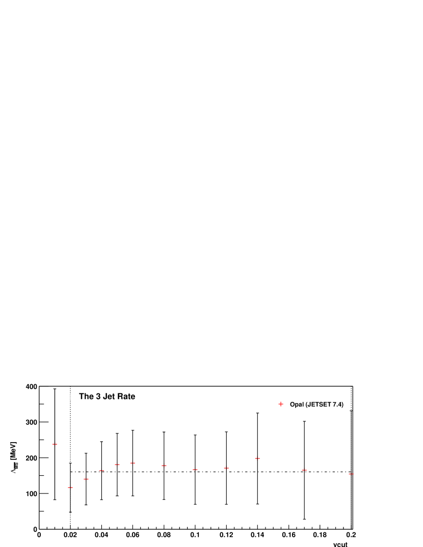
Figure 3: The 3 Jet Rate using OPAL data

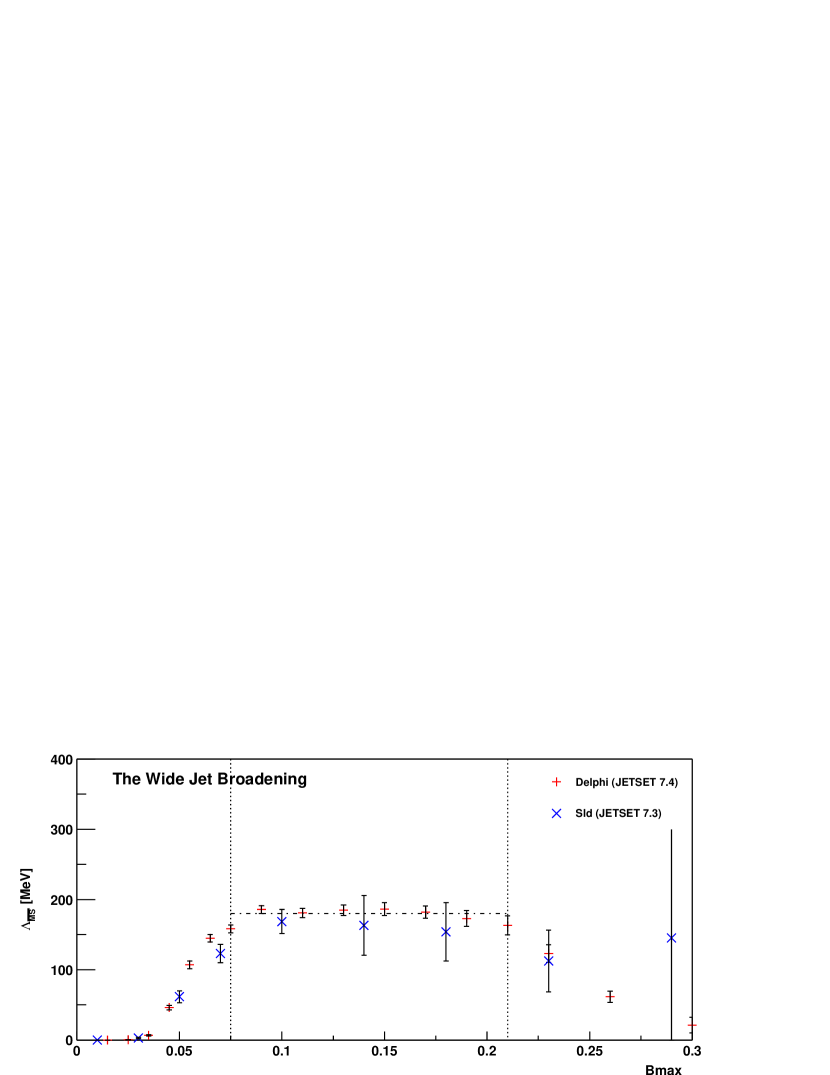
Figure 4: The Wide Jet Broadening using DELPHI and SLD data

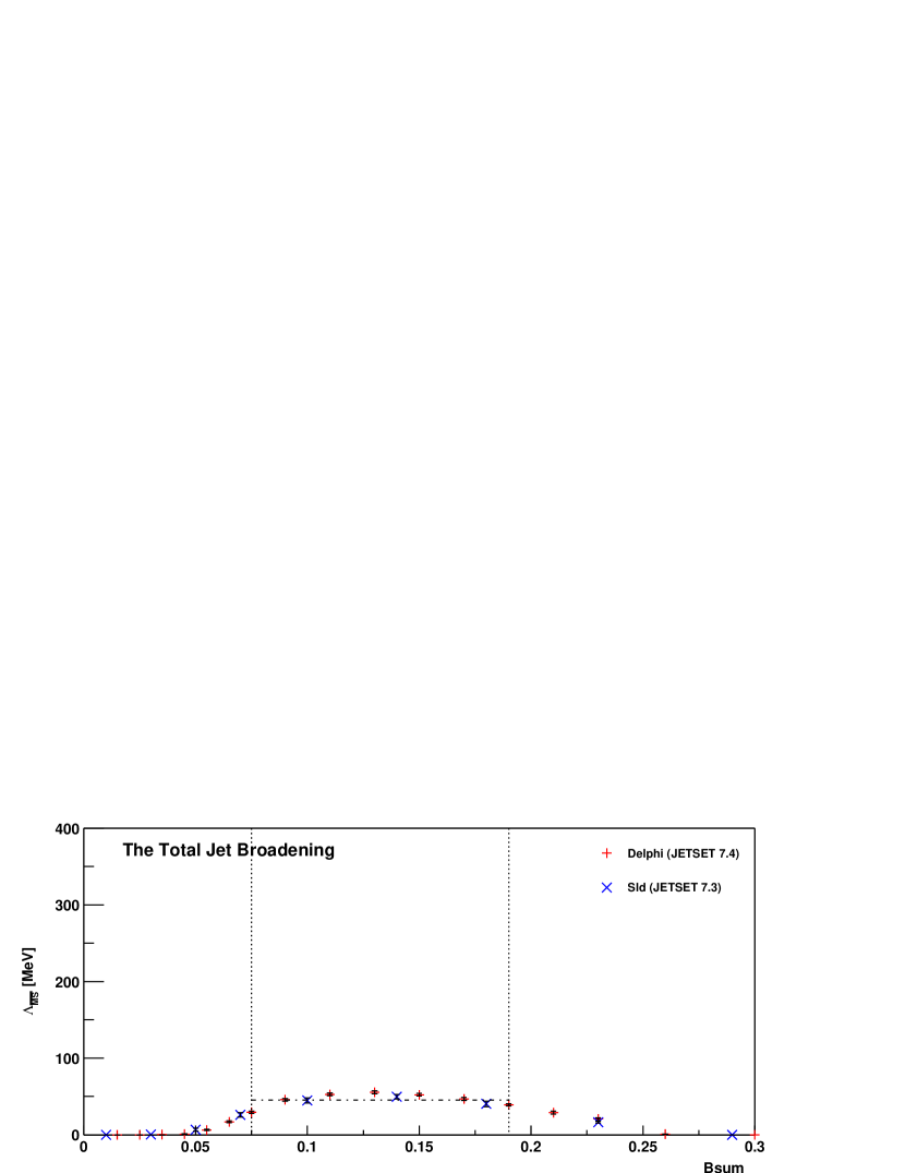
Figure 5: The Total Jet Broadening using DELPHI and SLD data

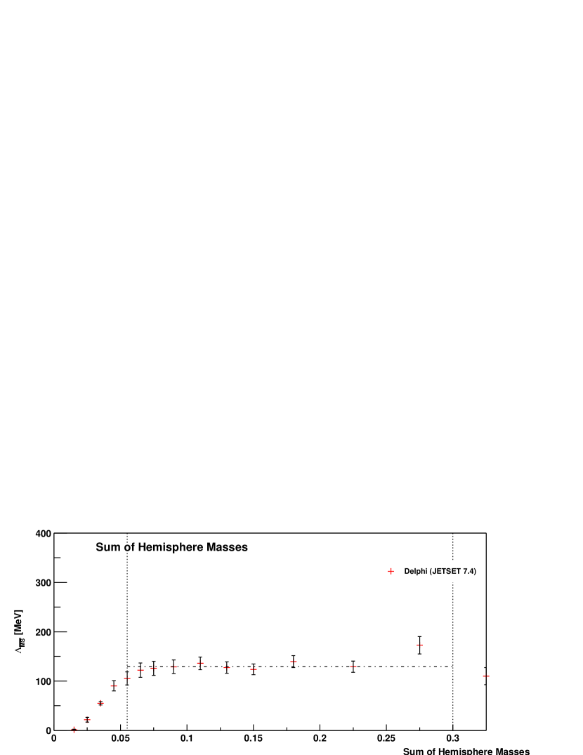
Figure 6: The Sum of Hemisphere Masses using DELPHI data

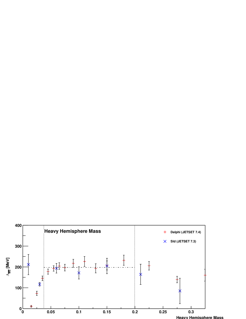
Figure 7: The Heavy Hemisphere Mass using DELPHI and SLD data

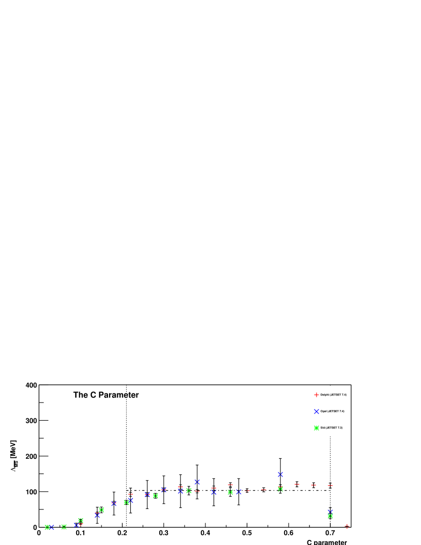
Figure 8: The C Parameter using DELPHI, OPAL and SLD data

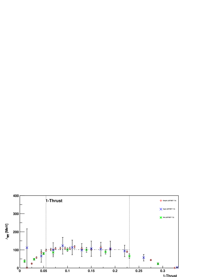
Figure 9: The 1-Thrust Parameter using DELPHI, OPAL and SLD data

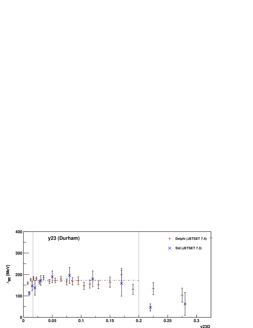
Figure 10: The $2\to 3$ Jet Transition Parameter using DELPHI and SLD data

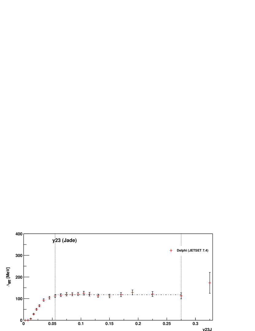
Figure 11: The $2\to 3$ Jet Transition Parameter using DELPHI data

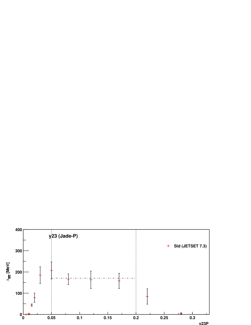
Figure 12: The $2\to 3$ Jet Transition Parameter using SLD data

Figure 13: The $2\to 3$ Jet Transition Parameter using SLD data

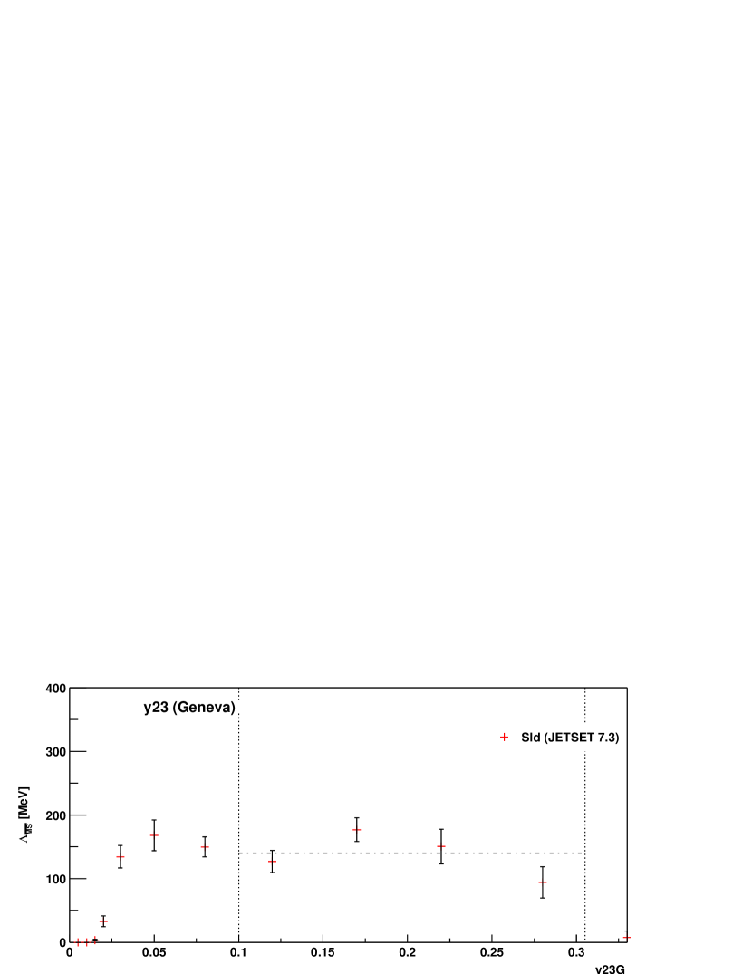
Figure 14: The $2\to 3$ Jet Transition Parameter using SLD data

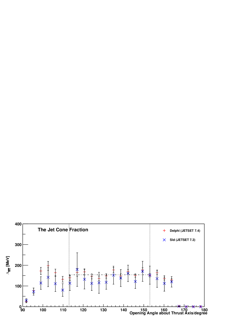
Figure 15: The Jet Cone Energy Fraction using DELPHI and SLD data

We note that some of the variables described in Sec. 3, in particular the difference in hemisphere masses, and the EEC and AEEC, have not been included, since the fitting criteria outlined earlier are not satisfied. For comparison the corresponding fitted values using data not corrected for hadronisation effects is given in Fig. 16. Without hadronisation corrections the fitted central values of ${\Lambda}_{\overline{{\mathrm{MS}}}}$ lie in the range between 50 MeV and 275 MeV. Including hadronisation corrections, reduces this range to between 100 MeV and 200 MeV. This factor of two uncertainty in ${\Lambda}_{\overline{{\mathrm{MS}}}}$ is then to be taken as providing an estimate of the likely size of remaining uncalculated NNLO and higher-order perturbative corrections. If we assume that for some of the observables ${\cal{G}}({\cal{R}}){\approx}1$, then the factor of two uncertainty in $\Lambda_{\overline{{\mathrm{MS}}}}\,$ can be translated into an estimate of the potential size of the two-loop NNLO RS-invariant ${\rho}_{2}$. Using Eq.(17) for ${\cal{G}}({\cal{R}})$ expanded as in Eq.(27), we see that ${\cal{G}}({\cal{R}}){\approx}2$, with the typical value of ${\cal{R}}{\approx}0.05$, corresponds to ${\rho}_{2}{\approx}50$. Without explicit NNLO calculations there is no rational basis for assigning a central value for $\Lambda_{\overline{{\mathrm{MS}}}}\,$ with an error. What one can say, however, is that inclusion of hadronisation corrections does reduce the spread in the extracted $\Lambda_{\overline{{\mathrm{MS}}}}\,$, and that this remaining spread indicates a value of ${\rho}_{2}$ which is not so large. We have no basis for estimating how big we might expect ${\rho}_{2}$ to be for these observables. We can note that for the $\mbox{e}^{+}\mbox{e}^{-}\,\!$ $R$-ratio which has been computed to NNLO, ${\rho}_{2}=-15.1$ for ${N_{f}}=5$ active flavours [15]. We can convert $\Lambda_{\overline{{\mathrm{MS}}}}\,$ to ${\alpha_{s}}({M_{Z}})$ using the two-loop beta-function equation. The corresponding values for hadronisation corrected data is given in Fig. 18.

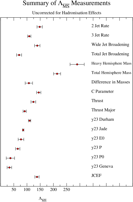
Figure 16: Summary of $\Lambda_{\overline{{\mathrm{MS}}}}$   measurements uncorrected for hadronisation effects.

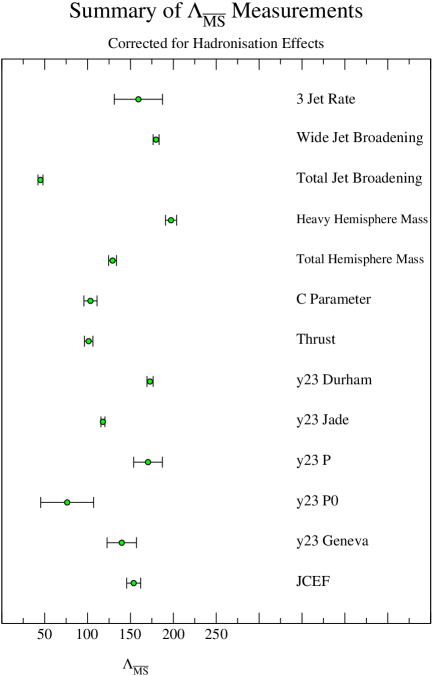
Figure 17: Summary of $\Lambda_{\overline{{\mathrm{MS}}}}$   measurements corrected for hadronisation effects.

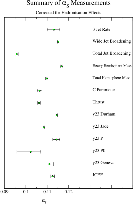
Figure 18: Summary of $\alpha_{s}$ measurements corrected for hadronisation effects.

We finally present the $\Lambda_{\overline{{\mathrm{MS}}}}\,$ values obtained by fitting to the data on four-jet observables. We use the DELPHI data of [45] in all cases. In this case we only analysed data uncorrected for hadronisation effects. The results for five variables are given in Fig. 19. With the exception of the Light Hemisphere Mass and the Narrow Jet Broadening the values are grouped between 150 and 200 MeV, reasonably consistent with those obtained from the three-jet observables. It may be that the Light Hemisphere Mass and Narrow Jet Broadening have rather large hadronisation corrections.

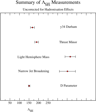
Figure 19: Summary of $\Lambda_{\overline{{\mathrm{MS}}}}$    measurements for four jet observables uncorrected for hadronisation effects.

5 Energy Dependence of the Thrust Distribution

In this section we consider how to include power corrections in our formalism. It is widely accepted that physical observables in general will be subject to “non-perturbative” power-like corrections in the hard interaction scale, $Q$. That is to say, there will be terms contributing to cross-sections that cannot be expanded out in the typical perturbative manner arising from expressions of the form

$$\left(\frac{\Lambda}{Q}\right)^{k}=\exp\left(\frac{-k}{b\,\alpha_{s}}\right).$$ (70)

Perturbative techniques cannot describe these terms accurately but have made attempts at predicting the leading behaviour to the power corrections via renormalon-inspired analysis [52, 53] and dispersive techniques [54]. Taking the generic form of these power corrections, we can alter our perturbative expansion for a dimensionless observable $\mathcal{R}$,

$$\mathcal{R}=a+r_{1}a^{2}+r_{2}a^{3}+\ldots+\frac{\lambda_{0}}{Q}(1+\lambda_{1}a+\lambda_{2}a^{2}+\lambda_{3}a^{3}+\ldots),$$ (71)

where we have assumed a leading power correction with exponent 1 (i.e. $\frac{1}{Q}$). To include these term in the analysis of Sec. 2, we must take the derivative with respect to $Q$. We may then rewrite Eq.(8) incorporating power corrections as

$$B({\mathcal{R}}(Q))=\frac{\mathrm{d}\mathcal{R}}{\mathrm{d}\ln Q} = -b\mathcal{R}^{2}(1+c\mathcal{R}+\rho_{2}\mathcal{R}^{2}+\rho_{3}\mathcal{R}^{3}+\ldots)$$ (72)

$$+ \kappa_{0}\mathcal{R}^{-c/b}e^{-1/b\mathcal{R}}(1+\kappa_{1}\mathcal{R}+\ldots)+\ldots,$$

where the $\kappa_{n}$ can be related to the $\lambda_{n}$. For example, the leading power correction coefficient gives a $-\lambda_{0}/Q$ contribution to the $\beta$-function. Using Eq.(12) to get $Q$ in the leading approximation of $\mathcal{R}$ we find,

$$Q\approx\Lambda_{\mathcal{R}}e^{1/b\mathcal{R}}(c\mathcal{R})^{c/b}.$$ (73)

Substituting this back in we obtain

$$\lambda=-\kappa_{0}e^{r_{1}(\mu=Q)/b}\left(\frac{b}{2}\right)^{c/b}\Lambda_{\overline{{\mathrm{MS}}}}\,\,,$$ (74)

where we have converted $\Lambda_{R}$ to $\Lambda_{\overline{{\mathrm{MS}}}}\,\,$. Having made the connection between $\kappa_{0}$ and $\lambda_{0}$ we may incorporate the power correction term into Eq.(24) via the $\mathcal{G}(\mathcal{R}(Q))$ function given in Eq.(17). Expanding out $\mathcal{G}(\mathcal{R}(Q))$ to the accuracy of NNLO and leading power corrections gives

$$\mathcal{G}(\mathcal{R}(Q))\simeq 1-\frac{\rho_{2}}{b}\mathcal{R}+\frac{\kappa_{0}}{b}\frac{e^{-1/b\mathcal{R}}}{\mathcal{R}^{2}}\mathcal{R}^{-c/b}.$$ (75)

Substituting this back into Eq.(24) we finally obtain

$$\Lambda_{\overline{{\mathrm{MS}}}}\,=Q\,{\cal{F}}({\mathcal{R}}(Q))\,\left(1-\frac{\rho_{2}}{b}\mathcal{R}+\frac{\kappa_{0}}{b}\frac{e^{-1/b\mathcal{R}}}{\mathcal{R}^{2}}\mathcal{R}^{-c/b}\right)\,{e}^{-r/b}\,{\left(\frac{2c}{b}\right)}^{c/b}\;.$$ (76)

We are fortunate enough to have experimental measurements of the thrust distribution at a wide variety of energy scales from PETRA to LEP2. We shall be considering the following data

• PETRA (Detector- Tasso, Facility-DESY) [55]

  • Centre of Mass Energies - 14, 22, 35 GeV

• PEP (Detector- Mark-II, Facility-SLAC) [56]

  • Centre of Mass Energy - 29GeV

• TRISTAN (Detector- Amy, Facility-KEK) [57]

  • Centre of Mass Energy - 52GeV

• SLC (Detector- SLD, Facility-SLAC)

  • Centre of Mass Energy - 91GeV

• LEP (Detectors- Aleph, Delphi, L3, Opal, Facility-CERN)

  • Centre of Mass Energy - 91GeV

Unfortunately as the LEP 2 data suffers from large errors due to poor statistics, we are forced to exclude it from the analysis. We would expect that the ${\Lambda_{\overline{{\mathrm{MS}}}}\,}$ directly extracted from Eq.(25) should approach the actual value as the energy increases, and sub-asymptotic effects become smaller with ${\mathcal{G}}(\mathcal{R})$ approaching more closely its asymptotic value of unity. This trend can indeed be seen from Figs. 20 and 21 (where we have removed the error bars for clarity). In the limit $1-T\to\frac{1}{3}$ we are faced once again with the problem of the kinematic end point dragging the value to zero. In the $1-T\to 0$ limit, large kinematic logarithms dominate from the emission of soft and collinear gluons. Clearly in between we see a “flattening” of the $\Lambda_{\overline{{\mathrm{MS}}}}$   value with $1-T$. This can be interpreted as higher order and power-like corrections having less influence, and hence the NLO approximation becoming more reliable.

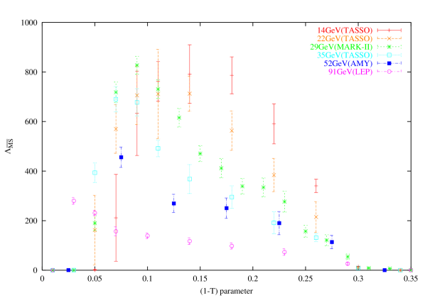
Figure 20: The Energy Dependence of $\Lambda_{\overline{{\mathrm{MS}}}}$  Measurements from the Thrust Distribution

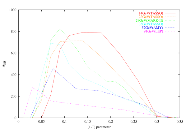
Figure 21: The Energy Dependence of $\Lambda_{\overline{{\mathrm{MS}}}}$  Measurements from the Thrust Distribution

It is possible to consider the formalism from a different perspective whereby we accept that $\Lambda_{\overline{{\mathrm{MS}}}}$   is a constant and that any deviations from its true value are due to higher order effects and power corrections. In this case we may then try to approximate these contributions by the leading terms as given by Eq. (76). In this section we highlight a simple mechanism for investigating these effects. We stress that this by no means provides a highly accurate estimate of these terms, but merely an indication of how important they are. We begin by rewriting Eq. (76) as

$$\kappa_{0}=M(\mathcal{R},r)\rho_{2}+C(\mathcal{R},r),$$ (77)

where $M(\mathcal{R},r)$ and $C(\mathcal{R},r)$ are known terms at NLO, having specified a value for $\Lambda_{\overline{{\mathrm{MS}}}}$  . This is simply the equation of a straight line in $(\kappa_{0},\rho_{2})$ space. Since these two quantities are $Q$-independent, we may plot the lines corresponding to different centre-of-mass energies and expect them to cross over at the solution. This is illustrated in Fig. 22 where we have taken a value of $\Lambda_{\overline{{\mathrm{MS}}}}\,\,=200$MeV. We have made no attempt to incorporate the errors, which for the LEP 2 data will be considerable. In all cases, the central value is taken. This naïve procedure does give a promising result, though. There appear to be two predominant localised cross-over regions where the lines appear to converge. These correspond to ${\rho}_{2}$ and ${\kappa}_{0}$ both small or ${\rho}_{2}{\approx}{-40}$ and ${\kappa}_{0}{\approx}-0.5$. Similar fits for the $<1-T>$ were performed in [58].

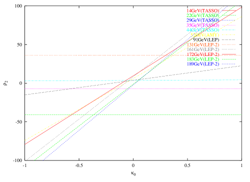
Figure 22: Fitting for the leading power correction ($\kappa_{0}$) and NNLO ($\rho_{2}$) using the thrust distribution at different energies. We use a value of $\Lambda_{\overline{{\mathrm{MS}}}}$  = 200MeV

6 Discussion and Conclusions

In this paper we have shown that one can directly relate QCD observables to the underlying dimensional transmutation parameter of the theory, leading to the relation of Eq.(24). This derivation does not require the specification of a renormalisation scale, or use of the convention-dependent renormalised coupling ${\alpha_{s}}(\mu)$. It is obtained simply by integrating up the obvious dimensional analysis statement of Eq.(3). This integration corresponds to identifying and resumming the complete set of ultra-violet logarithms of $Q$ which reside in the perturbative coefficients. In standard RG-improvement an infinite subset of these is tacitly omitted, and this results in the problematic scale-dependence of fixed-order predictions which plagues standard analyses. The only approximation in the present approach is the incomplete knowledge of the function ${\mathcal{G}}(\mathcal{R})$ which approaches unity for asymptotic $Q$, and deviates from it by two-loop (NNLO) sub-asymptotic effects characterised by the NNLO RS-invariant ${\rho}_{2}$, and by power corrections. Given that these are presently unknown for the QCD $\mbox{e}^{+}\mbox{e}^{-}\,\!$ jet observables we wished to analyse, the best we could do was to use Eq.(25), corresponding to the asymptotic expectation ${\mathcal{G}}({\mathcal{R}}(Q)){\approx}1$. As we discussed in Sec. 4, to avoid regions containing large kinematical logarithms arising in the two-jet limit, and kinematical endpoints, it was necessary to choose the range in the observable over which the fits to constant $\Lambda_{\overline{{\mathrm{MS}}}}\,$ were performed, rather carefully. Notwithstanding the fact that these fitting criteria are inevitably somewhat ad hoc, the procedure crucially avoids the additional scatter in extracted ${\Lambda_{\overline{{\mathrm{MS}}}}\,}$ values resulting from the arbitrary variation of the renormalization scale, which is customarily employed. One finds that the range of directly fitted $\Lambda_{\overline{{\mathrm{MS}}}}\,$ values obtained is significantly reduced using hadronisation corrected data (see Figs. 16 and 17). The remaining scatter in $\Lambda_{\overline{{\mathrm{MS}}}}\,$ values displayed in Fig. 17 is then to be attributed to the presence of uncalculated NNLO and higher-order sub-asymptotic effects in ${\mathcal{G}}({\mathcal{R}})$. The factor of two scatter in $\Lambda_{\overline{{\mathrm{MS}}}}\,$, roughly between $100$ and $200$ MeV, then corresponds on using the exponentiated form for ${\mathcal{G}}({\mathcal{R}})$ in Eq.(27), to an estimate $|{\rho}_{2}|{\approx}50$, indicating significant but not huge uncalculated two-loop effects. A firmer statement about the value of $\Lambda_{\overline{{\mathrm{MS}}}}\,$ is only possible once these effects have been computed. There seems to us to be no point in extracting a purported central value of $\Lambda_{\overline{{\mathrm{MS}}}}\,$ together with an error in the meantime.

In Sec. 5 we performed a complementary exercise in which, assuming a fixed value of ${\Lambda_{\overline{{\mathrm{MS}}}}\,}=200$MeV, the $Q$-dependence of the thrust distribution over the energy range from PETRA to LEP 2 was used to fit for the NNLO RS-invariant ${\rho}_{2}$ and power corrections. As seen from Fig. 21 as $Q$ increases the directly extracted $\Lambda_{\overline{{\mathrm{MS}}}}\,$ is reduced, and its distribution in thrust flattened, as would be expected if the sub-asymptotic effects contained in ${\mathcal{G}}({\mathcal{R}})$ are becoming smaller. The fits for ${\rho}_{2}$ and the ${\kappa}_{0}$, the parameter controlling $1/Q$ power corrections, shown in Fig. 22 reveal two possibilities. One corresponds to both ${\rho}_{2}$ and ${\kappa}_{0}$ small, and the other to ${\kappa}_{0}$ small and ${\rho}_{2}{\approx}-50$, a value consistent with that estimated from the scatter of $\Lambda_{\overline{{\mathrm{MS}}}}\,$ values in Fig. 17.

There are two major directions in which the formalism described here could be improved. The first would be to resum to all-orders large kinematical infra-red logarithms in the function ${\mathcal{G}}({\mathcal{R}})$. This would allow fitting over a much larger range in the observables. Whilst in principle straightforward a number of technical complications present themselves. The second would be to generalize the direct extraction of ${\Lambda_{\overline{{\mathrm{MS}}}}\,}$ to see how Eq.(24) is modified if one has massive quarks. We hope to report developments in both these areas in future papers.

References

- [1] S. Bethke, J. Phys. G26 (2000) R27.
- [2] A.X. El-Khadra, G. Hockney, A.S. Kronfeld and P.B. Mackenzie, Phys. Rev. Lett. 69 (1992) 729.
- [3] C. Davies et al., Phys. Rev. D56 (1997) 2755.
- [4] B. Alles, M. Campostrini, A. Feo and H. Panagopoulos, Phys. Lett. B324 433 ; M. Luscher and P. Weisz, Phys. Lett. B349 (1995) 165; Nucl. Phys. B452 (1995) 234.
- [5] R.K. Ellis, D.A. Ross and A.E. Terrano, Nucl. Phys. B178 (1981) 421.
- [6] P. Nason and Z. Kunszt, in Z Physics at LEP-1, Eds. G. Altarelli et al, CERN 89-08 (1989).
- [7] S. Catani and M.H. Seymour, Nucl. Phys. B485 (1997) 291; erratum ibid. B510 (1997) 503.
- [8] T. Sjöstrand, Comput. Phys. Commun. 82, (1994) 74.
- [9] G. Marchesini et al., Comput. Phys. Commun. 67, (1992) 465.
- [10] C.J. Maxwell, hep-ph/9908463.
- [11] C.J. Maxwell and A. Mirjalili, Nucl. Phys. B577 (2000) 209.
- [12] G. Grunberg, Phys. Lett. B95 (1980) 70.
- [13] G. Grunberg, Phys. Rev. D29 (1984) 2315.
- [14] P.M. Stevenson, Ann. Phys. 152 (1981) 383.
- [15] D.T. Barclay, C.J. Maxwell and M.T. Reader, Phys. Rev. D49 (1994) 3480.
- [16] V. Gupta, D.V. Shirkov and O.V. Tarasov, Int. J. Mod. Phys. A6 (1991) 3381.
- [17] P.M. Stevenson, Phys. Rev. D23 (1981) 2916.
- [18] A.J. Buras, E.G. Floratos, D.A. Ross and C.T. Sachrajda , Nucl. Phys. B131 (1977) 308; W.A. Bardeen, A.J. Buras, D.W. Duke and T. Muta, Phys. Rev. D18 (1978) 3998.
- [19] W.Celmaster and R.J. Gonsalves, Phys. Rev. D20 (1979) 1420.
- [20] S. Catani, L. Trantadue, G. Turnock and B.R. Webber, Nucl. Phys. B407 (1993) 3.
- [21] B. Magradze, Int.J.Mod.Phys. A15 (2000) 2715 and hep-ph/9808247.
- [22] Einan Gardi, Georges Grunberg and Marek Karliner, JHEP 07 (1998) 007.
- [23] W. Bernreuther and W. Wetzel, Nucl. Phys. B197 (1982) 228.
- [24] K.G. Chetyrkin, B.A. Kniehl and M. Steinhauser, Phys. Rev. Lett. 79 (1997) 2184.
- [25] S. Moretti, L. Lönnblad, and T. Sjöstrand, JHEP 08, (1998) 001.
- [26] JADE, S. Bethke et al., Phys. Lett. B213, (1988) 235.
- [27] N. Brown and W. Stirling, Z. Phys. C53, (1992) 629.
- [28] S. Catani, Y. L. Dokshitzer, M. Olsson, G. Turnock, and B. R. Webber, Phys. Lett. B269, (1991) 432.
- [29] S. Bethke, Z. Kunszt, D. E. Soper, and W. J. Stirling, Nucl. Phys. B370, (1992) 310; erratum ibid. Nucl. Phys. B523 (1998) 681.
- [30] S. Brandt, C. Peyrou, R. Sosnowski, and A. Wroblewski, Phys. Lett. 12, (1964) 57.
- [31] E. Farhi, Phys. Rev. Lett. 39, (1977) 1587.
- [32] D. P. Barber et al., Phys. Rev. Lett. 43, (1979) 830.
- [33] L. Clavelli, Phys. Lett. B85, (1979) 111.
- [34] Z. Kunszt, P. Nason, G. Marchesini, and B. R. Webber, Proceedings of the 1989 LEP Physics Workshop, Geneva, Swizterland, Feb 20, 1989.
- [35] S. Catani, G. Turnock, and B. R. Webber, Phys. Lett. B295, (1992) 269.
- [36] G. Parisi, Phys. Lett. B74, (1978) 65.
- [37] J. F. Donoghue, F. E. Low, and S.-Y. Pi, Phys. Rev. D20, (1979) 2759.
- [38] C. L. Basham, L. S. Brown, S. D. Ellis, and S. T. Love, Phys. Rev. Lett. 41, (1978) 1585.
- [39] C. L. Basham, L. S. Brown, S. D. Ellis, and S. T. Love, Phys. Rev. D19, (1979) 2018.
- [40] C. L. Basham, L. S. Brown, S. D. Ellis, and S. T. Love, Phys. Rev. D17, (1978) 2298.
- [41] Y. Ohnishi and H. Masuda, SLAC-PUB-6560.
- [42] SLD, K. Abe et al., Phys. Rev. D51, (1995) 692.
- [43] ALEPH, R. Barate et al., Phys. Rept. 294, (1998) 1.
- [44] DELPHI, P. Abreu et al., Eur. Phys. J. C14, (2000) 557.
- [45] DELPHI, P. Abreu et al., Z. Phys. C73, (1996) 11.
- [46] L3, B. Adeva et al., Z. Phys. C55, (1992) 39.
- [47] OPAL, P. D. Acton et al., Z. Phys. C55, (1992) 1.
- [48] W. T. Giele and E. W. N. Glover, Phys. Rev. D46, (1992) 1980.
- [49] J. M. Campbell, M. A. Cullen, and E. W. N. Glover, Eur. Phys. J. C9, (1999) 245.
- [50] D. E. Groom et al., Eur. Phys. J. C15, (2000) 1.
- [51] M. Schmelling, Phys. Scripta 51, (1995) 676.
- [52] A. H. Mueller, QCD: 20 Years Later, Aachen.
- [53] V. I. Zakharov, Nucl. Phys. B385, (1992) 452.
- [54] Y. L. Dokshitzer, G. Marchesini, and B. R. Webber, Nucl. Phys. B469, (1996) 93.
- [55] TASSO, W. Braunschweig et al., Z. Phys. C47, (1990) 187.
- [56] MARK-II, A. Petersen et al., Phys. Rev. D37, (1988) 1.
- [57] AMY, Y. K. Li et al., Phys. Rev. D41, (1990) 2675.
- [58] J. M. Campbell, E.W.N. Glover and C. J. Maxwell, Phys. Rev. Lett. 81 (1998) 1568.