THE CENTER SYMMETRY AND ITS SPONTANEOUS BREAKDOWN AT HIGH TEMPERATURES

The Euclidean action of non-Abelian gauge theories with adjoint dynamical charges (gluons or gluinos) at non-zero temperature $T$ is invariant against topologically non-trivial gauge transformations in the ${\sf Z\!\!\!Z}(N)_{c}$ center of the $SU(N)$ gauge group. The Polyakov loop measures the free energy of fundamental static charges (infinitely heavy test quarks) and is an order parameter for the spontaneous breakdown of the center symmetry. In $SU(N)$ Yang-Mills theory the ${\sf Z\!\!\!Z}(N)_{c}$ symmetry is unbroken in the low-temperature confined phase and spontaneously broken in the high-temperature deconfined phase. In 4-dimensional $SU(2)$ Yang-Mills theory the deconfinement phase transition is of second order and is in the universality class of the 3-dimensional Ising model. In the $SU(3)$ theory, on the other hand, the transition is first order and its bulk physics is not universal. When a chemical potential $\mu$ is used to generate a non-zero baryon density of test quarks, the first order deconfinement transition line extends into the $(\mu,T)$-plane. It terminates at a critical endpoint which also is in the universality class of the 3-dimensional Ising model. At a first order phase transition the confined and deconfined phases coexist and are separated by confined-deconfined interfaces. Similarly, the three distinct high-temperature phases of $SU(3)$ Yang-Mills theory are separated by deconfined-deconfined domain walls. As one approaches the deconfinement phase transition from the high-temperature side, a deconfined-deconfined domain wall splits into a pair of confined-deconfined interfaces and becomes completely wet by the confined phase. Complete wetting is a universal interface phenomenon that arises despite the fact that the bulk physics is non-universal. In supersymmetric $SU(3)$ Yang-Mills theory, a ${\sf Z\!\!\!Z}(3)_{\chi}$ chiral symmetry is spontaneously broken in the confined phase and restored in the deconfined phase. As one approaches the deconfinement phase transition from the low-temperature side, a confined-confined domain wall splits into a pair of confined-deconfined interfaces and thus becomes completely wet by the deconfined phase. This allows a confining string to end on a confined-confined domain wall as first suggested by Witten based on M-theory. Deconfined gluons and static test quarks are sensitive to spatial boundary conditions. For example, on a periodic torus the Gauss law forbids the existence of a single static quark. On the other hand, on a C-periodic torus (which is periodic up to charge conjugation) a single static quark can exist. As a paradoxical consequence of the presence of deconfined-deconfined domain walls, in very long C-periodic cylinders quarks are “confined” even in the deconfined phase.

1 Introduction and Summary

Understanding the non-perturbative dynamics of quarks and gluons is a highly non-trivial task. Since at low temperatures these particles are confined into hadrons, the quark and gluon fields that appear in the QCD Lagrangian do not provide direct insight into the non-perturbative physics of confinement. In the real world with light quarks confinement is accompanied by spontaneous chiral symmetry breaking and the presence of light pseudo-Goldstone pions. The pion fields that appear in the effective chiral Lagrangian do provide direct physical insight into the low-energy physics of QCD, but they do not shed light on the dynamical mechanism that is responsible for chiral symmetry breaking or confinement itself.

In order to gain some insight into the physics of confinement, it is very interesting to study QCD in extreme conditions of high temperature and large baryon chemical potential. Due to asymptotic freedom, confinement is then lost and we can hope to learn more about confinement by understanding how it turns into deconfinement. For the theory with light quarks this question is still very difficult to address from first principles, although a lot of interesting results have been obtained using lattice field theory as well as phenomenological models.

Here we decide to study a hypothetical world without dynamical quarks. Then the only dynamical color charge carriers are the gluons. Quarks appear only as infinitely heavy test charges that allow us to probe the gluon dynamics. In the resulting Yang-Mills theory confined and deconfined phases are easier to understand than in full QCD because they are characterized by distinct symmetry properties. As first pointed out by ’t Hooft $\!{}^{{\bf?}}$, the symmetry that distinguishes confinement from deconfinement is the ${\sf Z\!\!\!Z}(N)_{c}$ center symmetry of the $SU(N)$ gauge group.

The selection of topics covered in this article is strongly biased by the authors’ personal interests. Still, we hope that it will give a useful overview of the many interesting phenomena related to the center symmetry and its spontaneous breakdown. There is an extensive literature on the subject and we will not be able to discuss all important contributions. We like to apologize to those whose work will not be mentioned here.

1.1 Static Quarks and Dynamical Gluons

Gluons transform in the adjoint representation of $SU(N)$ and are ${\sf Z\!\!\!Z}(N)_{c}$ neutral. A single test quark transforms in the fundamental representation and carries a unit of ${\sf Z\!\!\!Z}(N)_{c}$ charge, while $N$ test quarks (forming a “test baryon”) are together ${\sf Z\!\!\!Z}(N)_{c}$ neutral. In Yang-Mills theory a confined phase is simply characterized by the fact that a non-zero ${\sf Z\!\!\!Z}(N)_{c}$ charge (for example, a single test quark) costs an infinite amount of free energy. In a deconfined phase, on the other hand, the free energy of a single static quark is finite. In full QCD this simple confinement criterion fails because in the presence of dynamical quarks the free energy of a single static test quark is always finite. This is because the color flux string emanating from the static quark can end in a dynamical anti-quark. The static-quark-dynamical-anti-quark meson has a finite free energy. In Yang-Mills theory, on the other hand, there are no dynamical quarks or anti-quarks and the string emanating from a test quark is absolutely unbreakable. Since it carries the ${\sf Z\!\!\!Z}(N)_{c}$ flux of the test quark, the string cannot end in a dynamical gluon which is ${\sf Z\!\!\!Z}(N)_{c}$ neutral. Instead it must go to infinity. Since the confining string has a non-zero tension (free energy per unit length) the static quark with the infinite flux string emanating from it costs an infinite amount of free energy.

Polyakov $\!{}^{{\bf?}}$ and Susskind $\!{}^{{\bf?}}$ were first to point out that the operator that describes a static quark is a Wilson loop closed around the periodic Euclidean time direction — the so-called Polyakov loop $\Phi$. The free energy $F$ of the test quark is determined by the thermal expectation value of the Polyakov loop as $\langle\Phi\rangle=\exp(-\beta F)$. Hence, in a confined phase in which $F=\infty$ one has $\langle\Phi\rangle=0$. This can be understood as follows. At low temperatures $T$ the extent $\beta=1/T$ of the Euclidean time direction is large. Then the Polyakov loop extends through many space-time regions that are essentially uncorrelated in color space. As a consequence, the Polyakov loop behaves essentially as a random variable and its thermal expectation value averages to zero. In the high-temperature deconfined phase, on the other hand, $F$ is finite and hence $\langle\Phi\rangle\neq 0$. In that case the Euclidean time direction is short and the Polyakov loop extends only through a small space-time region that is highly correlated in color space. Then the Polyakov loop orders and picks up a non-zero expectation value.

Under a twisted gauge transformation that is periodic up to an element $z$ of the center ${\sf Z\!\!\!Z}(N)_{c}$, the Polyakov loop changes by a factor $z$, while the action remains invariant. Consequently, the Polyakov loop is an order parameter for center symmetry breaking. A non-zero value of $\langle\Phi\rangle$ implies that the center symmetry is spontaneously broken. This is the case in the high-temperature deconfined phase. In the confined phase, on the other hand, the center symmetry is unbroken. This result is counter-intuitive, because one might expect spontaneous symmetry breaking to occur only at low temperatures. However, it should also not be too surprising because, for example, even the Ising model displays spontaneous symmetry breaking at high temperature when it is formulated in terms of dual variables. It should be noted that the center symmetry is absent in full QCD with dynamical quarks because their presence leads to explicit ${\sf Z\!\!\!Z}(3)_{c}$ breaking.

1.2 Phase Transitions and Interface Dynamics

As the order parameter that distinguishes confinement from deconfinement, the Polyakov loop plays a central role in understanding the physics of the high-temperature phase transition. In fact, just as the pion field of the effective chiral Lagrangian provides direct insight into the low-energy physics of QCD, an effective action for the Polyakov loop provides direct insight into the high-temperature physics close to the confinement-deconfinement phase transition. In the case of $SU(2)$ Yang-Mills theory, the Polyakov loop is represented by a real-valued scalar field in three dimensions with a $Z(2)_{c}$ symmetry. Hence, the effective theory for the Polyakov loop is a 3-d $\Phi^{4}$ theory. This theory is in the universality class of the 3-d Ising model. It was first noted by McLerran and Svetitsky $\!{}^{{\bf?}}$ and by Svetitsky and Yaffe $\!{}^{{\bf?}}$ that the second order phase transition in the 3-d Ising model has the same universal features as the deconfinement phase transition in the $SU(2)$ Yang-Mills theory. The first numerical lattice simulations indicating a second order $SU(2)$ deconfinement phase transition were performed in $\!{}^{{\bf?}}$. A detailed analysis of the critical exponents $\!{}^{{\bf?}}$ shows that they are indeed the same as in the 3-d Ising model. The lattice calculations of the value of the critical temperature have been extrapolated reliably to the continuum limit $\!{}^{{\bf?}}$.

In $SU(3)$ Yang-Mills theory the Polyakov loop is described by a complex-valued field $\Phi$ in three dimensions. The effective theory is again a 3-d $\Phi^{4}$ theory but now with a ${\sf Z\!\!\!Z}(3)_{c}$ symmetry. A lattice model with the same symmetries is the 3-d 3-state Potts model $\!{}^{{\bf?}}$ which is known to have a first order phase transition $\!{}^{{\bf?}}$. In $SU(3)$ Yang-Mills theory the deconfinement phase transition is therefore also expected to be first order $\!{}^{{\bf?}}$ so that the bulk physics is not universal. Lattice gauge theory has indeed provided detailed numerical evidence for a first order transition in $SU(3)$ Yang-Mills theory $\!{}^{{\bf?}}$. At a first order phase transition both phases coexist with each other and are separated by interfaces. For example, at the deconfinement phase transition the low-temperature confined phase and the high-temperature deconfined phase are separated by confined-deconfined interfaces. The simplest mechanism for the dynamics of a first order phase transition is bubble nucleation. For example, in boiling water bubbles of the gas phase form and grow in the liquid phase. Similarly, when one heats up a system of glueballs (confined gluons) beyond the temperature of the deconfinement phase transition, one expects the formation of bubbles of gluon plasma (deconfined gluons) which grow and ultimately fill the entire volume with deconfined phase. Due to the ${\sf Z\!\!\!Z}(3)_{c}$ symmetry, there are in fact three distinct deconfined phases. Hence, bubbles of different deconfined phases may nucleate independently in different parts of the volume. When these bubbles expand and collide they cannot coalesce and form a single bubble because they contain distinct types of deconfined phase. Consequently, when the phase transition is completed, we are left with different deconfined regions separated by deconfined-deconfined domain walls. These domain walls can exist at all temperatures above the phase transition point, while confined-deconfined interfaces are stable only at the phase transition. Deconfined-deconfined domain walls have a non-zero tension (free energy per unit area). Due to asymptotic freedom the domain wall tension can be calculated analytically at high temperatures using semi-classical methods $\!{}^{{\bf?}}$. The confined-deconfined interface tension, on the other hand, is accessible only to lattice simulations $\!{}^{{\bf?}}$ because the phase transition itself occurs at a temperature at which analytic methods based on asymptotic freedom are not applicable. It should be noted that in full QCD deconfined domains are unstable or at most meta-stable, because dynamical quarks break the center symmetry explicitly. The fate of a meta-stable deconfined domain in the early universe has been discussed $\!{}^{{\bf?}}$. Via a tunneling process it turns into the stable deconfined phase at temperatures around 10 TeV, i.e. much before it reaches the deconfinement phase transition at temperatures around 100 MeV.

When one cools the gluon plasma down below the phase transition temperature, one expects bubbles of the confined phase to nucleate in the bulk deconfined phase. These bubbles grow and ultimately fill the entire volume with confined (glueball) phase. Interestingly, in the presence of deconfined-deconfined domain walls there is a competing mechanism for generating the confined phase. Rather than nucleating in the deconfined bulk (which costs a large amount of confined-deconfined interface tension), it is energetically favorable for the confined phase to appear at a deconfined-deconfined domain wall, thus making use of the free energy provided by the domain wall tension $\!{}^{{\bf?}}$. In fact, the confined phase appears as a thin film that completely covers the domain wall. Hence, the deconfined-deconfined domain wall splits into a pair of confined-deconfined interfaces. Such phenomena are well known in condensed matter physics under the name of complete wetting. For example, in the human eye a film of liquid of tears completely wets the eye and thus separates it from the surrounding air. The alternative to complete wetting is incomplete wetting. Then lens shaped droplets of one phase appear at the domain wall separating two other phases. Interestingly, complete wetting is a universal phenomenon that occurs despite the fact that the phase transition is first order and the bulk physics is non-universal. In fact, complete wetting cannot occur at a second order bulk phase transition because it requires interfaces and thus phase coexistence. Complete wetting is characterized by a set of universal critical exponents which can be extracted from the effective 3-d ${\sf Z\!\!\!Z}(3)_{c}$ symmetric $\Phi^{4}$ theory for the Polyakov loop $\!{}^{{\bf?}}$.

The ${\sf Z\!\!\!Z}(3)_{c}$ center symmetry also plays an important role in the high-temperature physics of supersymmetric Yang-Mills theory. The supersymmetry partners of the gluons are adjoint Weyl fermions — the gluinos. Like gluons, gluinos are ${\sf Z\!\!\!Z}(3)_{c}$ neutral and their confinement or deconfinement can again be characterized by the value of the Polyakov loop. In particular, the ${\sf Z\!\!\!Z}(3)_{c}$ flux of an external fundamental test quark cannot end at a dynamical adjoint gluino and must hence go to infinity. In the confined phase this still costs an infinite amount of free energy. Besides the ${\sf Z\!\!\!Z}(3)_{c}$ symmetry, supersymmetric Yang-Mills theory has a ${\sf Z\!\!\!Z}(3)_{\chi}$ chiral symmetry. This symmetry is a remnant of the $U(1)_{R}$ symmetry that is explicitly broken down to ${\sf Z\!\!\!Z}(3)_{\chi}$ by an anomaly. In the low-temperature confined phase the ${\sf Z\!\!\!Z}(3)_{\chi}$ symmetry is spontaneously broken by the formation of a gluino condensate, while the ${\sf Z\!\!\!Z}(3)_{c}$ symmetry remains unbroken. At high temperatures one expects chiral symmetry to be restored and the ${\sf Z\!\!\!Z}(3)_{c}$ symmetry to be spontaneously broken due to deconfinement.

Due to the spontaneous breakdown of the ${\sf Z\!\!\!Z}(3)_{\chi}$ chiral symmetry there are three distinct confined phases in supersymmetric $SU(3)$ Yang-Mills theory that are distinguished by the value of the gluino condensate. Below the deconfinement phase transition these phases coexist and are separated by confined-confined domain walls. When such a domain wall is heated up to the phase transition temperature, one of the three high-temperature deconfined phases forms a complete wetting layer and the confined-confined domain wall splits into a pair of confined-deconfined interfaces $\!{}^{{\bf?}}$. The fact that the wetting layer consists of deconfined phase has interesting consequences. It allows a color flux string emanating from a static test quark to end on the wall because inside the deconfined wetting layer the flux spreads out and no longer costs infinite energy when transported to infinity. The phenomenon of strings ending on walls in supersymmetric Yang-Mills theory was first predicted by Witten in the context of M-theory $\!{}^{{\bf?}}$. The color flux string then appears as a fundamental string and the confined-confined domain wall manifests itself as a D-brane — a natural place for strings to end. Complete wetting provides a field theoretical explanation of this phenomenon.

1.3 The Center — A Subtle Symmetry

It should be noted that — unlike other symmetries — the center symmetry is not a symmetry of the Hamiltonian which describes the time evolution of the system. Instead, it is a symmetry of the transfer matrix which describes the spatial evolution of the system in thermal equilibrium. This subtle difference is at the origin of a controversy about the physical reality of distinct high-temperature phases and of deconfined-deconfined domain walls. It has been argued that these domain walls are just Euclidean field configurations (like instantons) which play no role in Minkowski space-time $\!{}^{{\bf?}}$. For example, in contrast to other topological excitations like monopoles or cosmic strings, one cannot expect a deconfined-deconfined domain wall to appear as an eigenstate of the theory’s Hamiltonian. This should not be too surprising because the deconfined phases themselves are thermal mixtures of pure states weighted by their Boltzmann factors. Of course, the entire spectrum of the Hamiltonian is completely independent of temperature. The spectrum of the transfer matrix, on the other hand, is very sensitive to the temperature which controls the size of the Euclidean time dimension. Despite the fact that deconfined-deconfined domain walls are not energy eigenstates, their presence in the thermally equilibrated gluon plasma has observable consequences — at least in Gedanken experiments. For example, the free energy of a static test quark in a large box filled with gluon plasma depends crucially on the shape of the box. This effect is due to the presence of distinct high-temperature phases and the deconfined-deconfined domain walls that separate them.

To study the free energy of a single static quark in a finite box one must choose appropriate boundary conditions. Standard periodic boundary conditions are inappropriate because — as a consequence of the ${\sf Z\!\!\!Z}(3)_{c}$ Gauss law — a single quark cannot even exist on a torus $\!{}^{{\bf?}}$. In a periodic volume the color flux emanating from a quark cannot go to infinity and must thus end in an anti-quark. The system as a whole is thus ${\sf Z\!\!\!Z}(3)_{c}$ neutral. In a finite periodic volume the expectation value of the Polyakov loop always vanishes even in the deconfined phase. As a consequence of the ${\sf Z\!\!\!Z}(3)_{c}$ symmetry there is tunneling between the three deconfined phases which averages the Polyakov loop to zero. Irrespective of the dynamics, a single quark in a periodic box always has infinite free energy just for topological reasons. An appropriate alternative are $C$-periodic boundary conditions which are periodic up to charge conjugation $\!{}^{{\bf?},{\bf?}}$. In that case, the $C$-periodic copy of a quark is an anti-quark outside the box that can absorb the flux. The $C$-periodic box itself contains just a single quark (or more precisely a superposition of a quark and an anti-quark) and is thus charged. $C$-periodic boundary conditions lead to an explicit breaking of the center symmetry that disappears only in the infinite volume limit $\!{}^{{\bf?}}$. As a consequence, the Polyakov loop no longer averages to zero and the free energy of a static quark becomes finite. In the confined phase the free energy goes to infinity in the infinite volume limit, while it remains finite in the deconfined phase. $C$-periodic boundary conditions are useful in a Gedanken experiment that demonstrates the physically observable consequences of the presence of deconfined-deconfined domain walls. In the deconfined phase a single quark in a cubic $C$-periodic volume has a finite free energy. In a long cylindrical volume, on the other hand, the free energy increases with the length of the cylinder $\!{}^{{\bf?}}$. Hence, the quark is “confined” even in the deconfined phase, despite the fact that there is no flux string emanating from the quark. “Confinement” in the deconfined phase is a consequence of distinct deconfined phases being aligned along the long direction of the cylinder. This is an indication that spontaneous center symmetry breaking is not just a Euclidean artifact. The sensitivity of the quark’s free energy to the shape of the spatial volume is observable in Minkowski space-time and is characteristic for a spontaneously broken ${\sf Z\!\!\!Z}(3)_{c}$ symmetry. Other interesting subtleties of the center symmetry are related to the way it arises in gauge-fixed formulations of the theory $\!{}^{{\bf?}}$ and to the ’t Hooft loop order parameter $\!{}^{{\bf?}}$.

1.4 Organization of the Rest of the Article

The rest of this article contains a detailed and more mathematical discussion of the topics outlined in the introduction. Section 2 describes the bulk physics of gluons at high temperature. In particular, effective theories for the Polyakov loop are constructed at non-zero temperature and at non-zero chemical potential for static quarks. The nature of confined and deconfined phases is discussed and the transitions between them are characterized. In section 3 we study the properties and the dynamics of interfaces separating coexisting phases of confined and deconfined gluons and gluinos. In particular, the universal phenomenon of complete wetting is explored using effective theories for the Polyakov loop. Section 4 deals with static quarks at finite volume and the paradoxical “confinement” in the deconfined phase. Finally, section 5 contains our conclusions.

2 Gluons at High Temperatures

In this section we introduce $SU(N)$ pure Yang-Mills gauge theory at non-zero temperature. We discuss the problem in the language of continuum field theory but ignore the subtleties that arise in the regularization of ultraviolet divergences. Consequently, the resulting expressions are sometimes rather formal. We are interested in non-perturbative questions that can in general not be fully addressed directly in the continuum. Using the lattice regularization, it is straightforward to replace the formal quantities by completely well defined mathematical expressions. We prefer not to do this here because mathematical rigor might obscure the basic physics that can be well understood in continuum field theory language. Still, we like to emphasize that our understanding of the center symmetry and its spontaneous breakdown is to a large extent due to studies in lattice field theory — the most powerful tool for understanding non-perturbative field theory from first principles.

2.1 Path Integral and Euclidean Action

Let us consider a system of gluons at a non-zero temperature $T=1/\beta$. Its partition function is given by

$$Z=\mbox{Tr}\ [\exp(-\beta H)P].$$ (1)

Here $H$ is the Yang-Mills Hamilton operator and $P$ is a projection operator that enforces the Gauss law. It reduces the trace over all states to those that are gauge invariant and hence physical. We note that $\exp(-\beta H)$ is similar to the time-evolution operator $\exp(-iHt)$, except that $\beta$ plays the role of an imaginary (or Euclidean) time interval $it$. However, in order to motivate path integrals in Euclidean time, there is no need to start out in real Minkowski time and then Wick-rotate. Our starting point is equilibrium thermodynamics which makes no reference to real time evolution and puts us directly into Euclidean space-time. One can write a path integral expression for the partition function,

$$Z=\int DA\ \exp(-S[A]),$$ (2)

where

$$S[A]=\frac{1}{2g^{2}}\int_{0}^{\beta}dx_{4}\int d^{3}x\ \mbox{Tr}F_{\mu\nu}F_{\mu\nu}$$ (3)

is the Euclidean action. Here $g$ is the gauge coupling and

$$F_{\mu\nu}=\partial_{\mu}A_{\nu}-\partial_{\nu}A_{\mu}+[A_{\mu},A_{\nu}]$$ (4)

is the field strength resulting from the anti-Hermitian non-Abelian vector potential

$$A_{\mu}=iA_{\mu}^{a}\lambda^{a}.$$ (5)

The $SU(N)$ gluon field is described by $N^{2}-1$ real-valued functions $A_{\mu}^{a}(x)$ (with $a\in\{1,2,...,N^{2}-1\}$) of the Euclidean space-time points $x=(\vec{x},x_{4})$. The $\lambda^{a}$ are the $N^{2}-1$ Hermitian generators of the $SU(N)$ algebra in the fundamental representation. As a consequence of the trace in eq.(1), the measure $DA$ of the path integral contains fields that obey periodic boundary conditions,

$$A_{\mu}(\vec{x},x_{4}+\beta)=A_{\mu}(\vec{x},x_{4}),$$ (6)

in the Euclidean time direction. In the path integral the projection operator $P$ that enforces the Gauss law manifests itself as the integration over the time-like vector potentials $A_{4}$.

2.2 Gauge Invariance and Center Symmetry

The action of eq.(3) is invariant under gauge transformations

$${}^{g}\!A_{\mu}=g(A_{\mu}+\partial_{\mu})g^{\dagger},$$ (7)

with $g(x)\in SU(N)$, under which the field strength transforms as

$${}^{g}\!F_{\mu\nu}=gF_{\mu\nu}g^{\dagger}.$$ (8)

In order to maintain the boundary condition eq.(6) for the vector potential, we first consider gauge transformations that are strictly periodic in Euclidean time

$$g(\vec{x},x_{4}+\beta)=g(\vec{x},x_{4}).$$ (9)

Every physical quantity must be invariant under these gauge transformations. However, in addition there are topologically non-trivial transformations $\!{}^{{\bf?}}$ that are periodic up to a constant twist matrix $h\in SU(N)$

$$g(\vec{x},x_{4}+\beta)=hg(\vec{x},x_{4}).$$ (10)

When such a transformation is applied to a strictly periodic vector potential $A_{\mu}$ it turns into

$${}^{g}\!A_{\mu}(\vec{x},x_{4}+\beta) = g(\vec{x},x_{4}+\beta)(A_{\mu}(\vec{x},x_{4}+\beta)+\partial_{\mu})g(\vec{x},x_{4}+\beta)^{\dagger}$$ (11)

$$= hg(\vec{x},x_{4})(A_{\mu}(\vec{x},x_{4})+\partial_{\mu})g(\vec{x},x_{4})^{\dagger}h^{\dagger}$$

$$= h\ ^{g}\!A_{\mu}(\vec{x},x_{4})h^{\dagger}.$$

The gauge transformed vector potential ${}^{g}\!A_{\mu}$ obeys the boundary condition eq.(6) only if

$$h\ ^{g}\!A_{\mu}(\vec{x},x_{4})h^{\dagger}=\ ^{g}\!A_{\mu}(\vec{x},x_{4}),$$ (12)

which is the case only if $h$ commutes with ${}^{g}\!A_{\mu}$. This limits us to twist matrices $h$ in the center ${\sf Z\!\!\!Z}(N)_{c}$ of the gauge group $SU(N)$. The elements of the center commute with all group elements and are multiples of the unit matrix

$$h=z{\sf 1\!\!1},\ z=\exp(2\pi in/N),\ n\in\{1,2,...,N\}.$$ (13)

It is important to note that the ${\sf Z\!\!\!Z}(N)$ symmetry gets explicitly broken in the presence of dynamical fields that transform in the fundamental representation of $SU(N)$. For example, quark fields transform as

$${}^{g}\!\Psi=g\Psi,$$ (14)

and are anti-periodic in Euclidean time,

$$\Psi(\vec{x},x_{4}+\beta)=-\Psi(\vec{x},x_{4}).$$ (15)

Hence, under a twisted transformation they transform into

$${}^{g}\!\Psi(\vec{x},x_{4}+\beta)=g(\vec{x},x_{4}+\beta)\Psi(\vec{x},x_{4}+\beta)=-zg(\vec{x},x_{4})\Psi(\vec{x},x_{4})=-z\ ^{g}\!\Psi(\vec{x},x_{4}).$$ (16)

To maintain the boundary condition eq.(15) one must restrict oneself to $z=1$ so that the center symmetry disappears.

The twisted transformations of eq.(10) represent a global ${\sf Z\!\!\!Z}(N)_{c}$ symmetry of the action of eq.(3). Although the action is ${\sf Z\!\!\!Z}(N)_{c}$ invariant, other physical quantities need not necessarily be invariant under the center symmetry transformations. In particular, unlike the local $SU(N)$ gauge symmetry, the global ${\sf Z\!\!\!Z}(N)_{c}$ symmetry can break spontaneously and should not be considered as a subgroup of the local gauge group. It should be pointed out that the center symmetry is a symmetry of the Euclidean action, not of the Hamiltonian. While the Hamiltonian acts at a given instant in time, the ${\sf Z\!\!\!Z}(N)_{c}$ transformations are characterized by non-trivial boundary conditions in Euclidean time and thus affect the entire time evolution. Hence, it is meaningless to ask how states in the physical Hilbert space transform under the center symmetry. Instead, the center symmetry is a symmetry of the spatial transfer matrix — the analog of the Hamiltonian that describes the evolution of the system in a spatial direction. The spatial transfer matrix also acts on a Hilbert space (however, not on the usual one) and the states in that space have definite transformation properties under ${\sf Z\!\!\!Z}(N)_{c}$. In fact, at non-zero temperature the spatial transfer matrix is at least as useful as the Hamiltonian. While the spectrum of the Hamiltonian is by definition independent of temperature, the spectrum of the transfer matrix is sensitive to the temperature and, for example, contains valuable information about phase transitions.

2.3 The Polyakov Loop as an Order Parameter for Deconfinement

As we have seen, dynamical fields that transform in the fundamental representation break the ${\sf Z\!\!\!Z}(N)_{c}$ symmetry explicitly. Here we limit ourselves to cases where such fields are not present. Still, even then one can use static fundamental charges to probe the physics of the adjoint dynamical fields. Static fundamental charges (infinitely heavy test quarks) are described by the Polyakov loop (a Wilson loop closed around the periodic Euclidean time direction) $\!{}^{{\bf?},{\bf?}}$

$$\Phi(\vec{x})=\mbox{Tr}\ {\cal P}\exp(\int_{0}^{\beta}dx_{4}\ A_{4}(\vec{x},x_{4})).$$ (17)

Here ${\cal P}$ denotes path ordering of the exponential. The Polyakov loop is a complex scalar field that depends on the spatial position $\vec{x}$ of the static color source. In the special case of two colors ($N=2$) the Polyakov loop is always real. The Polyakov loop transforms non-trivially under twisted ${\sf Z\!\!\!Z}(N)_{c}$ transformations

$${}^{g}\!\Phi(\vec{x}) = \mbox{Tr}\ {\cal P}\exp(\int_{0}^{\beta}dx_{4}\ ^{g}\!A_{4}(\vec{x},x_{4}))$$ (18)

$$= \mbox{Tr}\ [g(\vec{x},x_{4}+\beta){\cal P}\exp(\int_{0}^{\beta}dx_{4}\ A_{4}(\vec{x},x_{4}))g(\vec{x},x_{4})^{\dagger}]$$

$$= \mbox{Tr}\ [zg(\vec{x},x_{4}){\cal P}\exp(\int_{0}^{\beta}dx_{4}\ A_{4}(\vec{x},x_{4}))g(\vec{x},x_{4})^{\dagger}]=z\Phi(\vec{x}).$$

On the other hand, it is invariant under strictly periodic gauge transformations (with $z=1$) as it should as a gauge invariant physical quantity.

The partition function of a system of gluons in the presence of a static infinitely heavy test quark is given by

$$Z_{Q}=\int DA\ \Phi(\vec{x})\exp(-S[A]).$$ (19)

The thermal expectation value of the Polyakov loop,

$$\langle\Phi\rangle=\frac{1}{Z}\int DA\ \Phi(\vec{x})\exp(-S[A])=\frac{Z_{Q}}{Z}=\exp(-\beta F),$$ (20)

is the ratio of the partition functions of the gluon systems with and without the external color source and hence measures the free energy $F$ of the external static quark. At low temperatures color is confined and the free energy of a single quark is infinite ($F=\infty$). Consequently, in the confined phase $\langle\Phi\rangle=0$. At high temperatures, on the other hand, asymptotic freedom suggests that quarks and gluons become deconfined. Then $F$ is finite and $\langle\Phi\rangle=\Phi_{0}\neq 0$ in the deconfined phase. Since $\Phi$ transforms non-trivially under center symmetry transformations, a non-zero expectation value $\Phi_{0}$ implies that the ${\sf Z\!\!\!Z}(N)_{c}$ symmetry is spontaneously broken in the high-temperature deconfined phase. It is unusual that a symmetry that is intact at low temperatures gets spontaneously broken at high temperatures. However, we should keep in mind that the center symmetry is a symmetry of the spatial transfer matrix — not a symmetry of the Hamiltonian. In fact it is easy to understand why the center symmetry must break spontaneously in the high-temperature limit $\beta\rightarrow 0$. In this limit the integral in eq.(17) extends over shorter and shorter Euclidean time intervals and hence $\Phi_{0}\rightarrow\mbox{Tr}{\sf 1\!\!1}=N$.

2.4 Effective Actions for the Polyakov Loop

To investigate the deconfinement phase transition it is instructive to consider effective theories for the Polyakov loop. In principle, one can imagine to integrate out the gluon fields and derive the effective action for the Polyakov loop directly from the underlying Yang-Mills theory

$$\exp(-S[\Phi])=\int DA\ \delta[\Phi(\vec{x})-\mbox{Tr}\ {\cal P}\exp(\int_{0}^{\beta}dx_{4}\ A_{4}(\vec{x},x_{4}))]\exp(-S[A]).$$ (21)

Here the $\delta$-functional ensures that $\Phi$ obeys eq.(17). The resulting effective action is nonlocal and impossible to compute in practice. Fortunately this is not even necessary. To gain some qualitative insight into the nature of the deconfinement phase transition it is sufficient to construct simple effective theories that have the desired symmetry properties and to study their properties. This approach is particularly fruitful when one wants to study a universal phenomenon that is common to the Yang-Mills theory and to much simpler models. All universal aspects of this phenomenon can then be studied in a simple effective theory for the Polyakov loop. Universal behavior is naturally associated with second order phase transitions. Then a physical correlation length becomes infinitely large and the short-distance details of the dynamics become irrelevant. What matters are only the dimensionality of space and the symmetry properties of the order parameter.

Let us first construct a simple effective theory for the Polyakov loop in $SU(2)$ pure gauge theory. Because the trace of an $SU(2)$ matrix is always real, the Polyakov loop $\Phi(\vec{x})$ is then a real-valued field in three dimensions. It transforms non-trivially under the ${\sf Z\!\!\!Z}(2)_{c}$ center transformations as ${}^{g}\!\Phi=z\Phi$ with $z=\pm 1$. Consequently, it is natural to consider the action

$$S[\Phi]=\int d^{3}x\ [\frac{1}{2}\partial_{i}\Phi\partial_{i}\Phi+V(\Phi)]$$ (22)

with a ${\sf Z\!\!\!Z}(2)_{c}$ invariant potential

$$V(\Phi)=a\Phi^{2}+c\Phi^{4}.$$ (23)

Stability of the problem requires $c>0$. For $a>0$ the potential has a single minimum at $\Phi=0$ that corresponds to the low-temperature confined phase. For $a<0$, on the other hand, there are two degenerate minima at $\Phi=\pm\Phi_{0}=\pm\sqrt{a/2c}$ corresponding to two high-temperature deconfined phases. The phase transition happens at $a=0$ and then $\Phi_{0}\rightarrow 0$ indicating a second order phase transition. Hence, for $SU(2)$ pure gauge theory one indeed expects universal behavior at the deconfinement phase transition $\!{}^{{\bf?},{\bf?}}$. A simple lattice model with the same spatial dimension and the same ${\sf Z\!\!\!Z}(2)$ symmetry is the 3-dimensional Ising model. Indeed, detailed lattice gauge theory studies have shown that the deconfinement phase transition of the $SU(2)$ Yang-Mills theory is second order $\!{}^{{\bf?}}$ and in the universality class of the 3-d Ising model $\!{}^{{\bf?}}$. Since the order parameter vanishes continuously, at a second order phase transition the various phases become indistinguishable at the transition. The lattice calculations also give the ratio of the critical temperature $T_{c}$ and the square root of the zero-temperature string tension $\sigma$ as $T_{c}/\sqrt{\sigma}=0.69(1)$ $\!{}^{{\bf?}}$.

For three colors ($N=3$) the situation is different. First of all, the Polyakov loop $\Phi=\Phi_{1}+i\Phi_{2}$ is now a complex scalar field with real part $\Phi_{1}$ and imaginary part $\Phi_{2}$. Consequently, besides the ${\sf Z\!\!\!Z}(3)$ center symmetry, we now must also consider the charge conjugation symmetry. Charge conjugation replaces the non-Abelian vector potential by its complex conjugate

$${}^{C}\!A_{\mu}=A_{\mu}^{*}.$$ (24)

Accordingly the Polyakov loop also turns into its complex conjugate

$${}^{C}\!\Phi(\vec{x}) = \mbox{Tr}\ {\cal P}\exp(\int_{0}^{\beta}dx_{4}\ ^{C}A_{4}(\vec{x},x_{4}))$$ (25)

$$= \mbox{Tr}\ {\cal P}\exp(\int_{0}^{\beta}dx_{4}\ A_{4}(\vec{x},x_{4})^{*})=\Phi(\vec{x})^{*}.$$

The natural candidate for an effective action now is

$$S[\Phi]=\int d^{3}x\ [\frac{1}{2}\partial_{i}\Phi^{*}\partial_{i}\Phi+V(\Phi)],$$ (26)

with a ${\sf Z\!\!\!Z}(3)_{c}$ and charge conjugation invariant potential, i.e.

$$V(z\Phi)=V(\Phi),\ V(\Phi^{*})=V(\Phi).$$ (27)

The most general quartic potential that obeys these symmetries is given by

$$V(\Phi)=a|\Phi|^{2}+b\Phi_{1}(3\Phi_{2}^{2}-\Phi_{1}^{2})+c|\Phi|^{4}.$$ (28)

Again, in order to have a stable system we need $c>0$. For $a>0$ the system has a minimum at $\Phi_{1}=\Phi_{2}=0$ corresponding to the confined phase. For $0<a<9b^{2}/32c$ there is another minimum at

$$\Phi_{1}=\Phi_{0}=\frac{3b+\sqrt{9b^{2}-32ac}}{8c},\ \Phi_{2}=0,$$ (29)

which has two other ${\sf Z\!\!\!Z}(3)_{c}$ copies. We denote the four minima by

$$\Phi^{(1)}=\Phi_{0},\ \Phi^{(2)}=\frac{1}{2}(-1+i\sqrt{3})\Phi_{0},\ \Phi^{(3)}=\frac{1}{2}(-1-i\sqrt{3})\Phi_{0},\ \Phi^{(4)}=0.$$ (30)

The first three minima correspond to the three high-temperature deconfined phases. For $b^{2}=4ac$ all four minima are degenerate. This corresponds to the phase transition temperature. However, in contrast to the $SU(2)$ case, at the phase transition we now have $\Phi_{0}=\sqrt{a/c}=b/2c\neq 0$ which corresponds to a first order phase transition. At a first order phase transition one does not have universal behavior in the bulk because the bulk correlation length remains finite and the short distance details of the dynamics remain important at the phase transition. A simple lattice model in the same spatial dimension and with the same global symmetries as the $SU(3)$ pure gauge theory is the 3-d 3-state Potts model $\!{}^{{\bf?}}$ which indeed has a first order phase transition $\!{}^{{\bf?}}$. Furthermore, detailed numerical studies in lattice gauge theory have shown that the deconfinement phase transition in $SU(3)$ Yang-Mills theory is also first order $\!{}^{{\bf?}}$. In this case the ratio of the critical temperature and the square root of the string tension is $T_{c}/\sqrt{\sigma}=0.64(1)$.

2.5 Gluons in a Background of Static Quarks

As we have seen, the partition function of a system of gluons in the presence of a single static quark at position $\vec{x}$ is given by eq.(19). Similarly, the gluon partition function in the presence of a single anti-quark is

$$Z_{\overline{Q}}=\int DA\ \Phi(\vec{x})^{*}\exp(-S[A]).$$ (31)

Consequently, the partition function of a system of gluons in the background of $n$ static quarks and $\overline{n}$ static anti-quark takes the form

$$Z_{n,\overline{n}}=\int DA\ \frac{1}{n!}[\int d^{3}x\ \Phi(\vec{x})]^{n}\frac{1}{\overline{n}!}[\int d^{3}y\ \Phi(\vec{y})^{*}]^{\overline{n}}\exp(-S[A]).$$ (32)

Here we have integrated over the positions $\vec{x}$ of quarks and $\vec{y}$ of anti-quarks. The factors $n!$ and $\overline{n}!$ take into account that quarks as well as anti-quarks are indistinguishable particles. We consider quarks of mass $M$ with quark chemical potential $\mu$ that couples to the baryon number $B=(n-\overline{n})/3$ and thus obtain

$$Z(\mu) = \sum_{n,\overline{n}}Z_{n,\overline{n}}\exp(-\beta M(n+\overline{n}))\exp(\beta\mu(n-\overline{n}))$$ (33)

$$= \int DA\sum_{n,\overline{n}}\frac{1}{n!}[\int d^{3}x\ \Phi(\vec{x})]^{n}\exp(-\beta(M-\mu)n)$$

$$\times \frac{1}{\overline{n}!}[\int d^{3}y\ \Phi(\vec{y})^{*}]^{\overline{n}}\exp(-\beta(M+\mu)\overline{n})\exp(-S[A])$$

$$= \int DA\exp[\int d^{3}x\ \Phi(\vec{x})\exp(-\beta(M-\mu))]$$

$$\times \exp[\int d^{3}y\ \Phi(\vec{y})^{*}\exp(-\beta(M+\mu))]\exp(-S[A]).$$

Consequently, the effective action for the gluons now takes the form

$$S_{eff}[A]=S[A]-\int d^{3}x\ [\Phi(\vec{x})\exp(-\beta(M-\mu))+\Phi(\vec{x})^{*}\exp(-\beta(M+\mu))].$$ (34)

As expected in the presence of fundamental charges, the additional terms in the effective action break the center symmetry explicitly. In the presence of the chemical potential, the effective action is in general complex. The $SU(2)$ case is exceptional because then the Polyakov loop and hence the effective action take real values. The action is real even in the $SU(N)$ case for purely imaginary values of the chemical potential. In that case, $\mu=iB_{4}$ enters the action as a constant vector potential $B_{4}$ in the 4-direction that couples to the baryon number. A real chemical potential, on the other hand, enters the action as a purely imaginary vector potential. Taking the limit $M,\mu\rightarrow\infty$ with $M-\mu$ finite we obtain

$$S_{eff}[A]=S[A]-\int d^{3}x\ \Phi(\vec{x})\exp(-\beta(M-\mu)).$$ (35)

The chemical potential favors positive real values of $\Phi$.

In the simple $\Phi^{4}$ model for the $SU(3)$ Polyakov loop the chemical potential enters the effective potential as

$$V(\Phi)=a|\Phi|^{2}+b\Phi_{1}(3\Phi_{2}^{2}-\Phi_{1}^{2})+c|\Phi|^{4}-h\Phi,$$ (36)

where $h$ represents $\exp(-\beta(M-\mu))$. At non-zero $h$ the deconfined phase $d^{(1)}$ with a real valued Polyakov loop is favored while the other two deconfined phases are suppressed. The deconfined phase $d^{(1)}$ coexists with the confined phase along a first order transition line that terminates in a critical endpoint. Since the ${\sf Z\!\!\!Z}(3)_{c}$ symmetry is explicitly broken in the presence of the chemical potential, at non-zero $h$ the Polyakov loop is non-zero even in the confined phase. We denote the values of the Polyakov loop in the confined and the deconfined phase by $\Phi^{(c)}$ and $\Phi^{(d)}$, respectively. Along the first order transition line at which the confined and the deconfined phase coexist, the potential (at $\Phi_{2}=0$) can then be written as

$$V(\Phi)=c(\Phi_{1}-\Phi^{(d)})^{2}(\Phi_{1}-\Phi^{(c)})^{2}+V_{0}.$$ (37)

Comparing eq.(36) and eq.(37) one derives a condition for the location of the first order phase transition line

$$\frac{4ac}{b^{2}}-1=\frac{8c^{2}}{b^{3}}h.$$ (38)

It is non-trivial to analyze the phase diagram with lattice field theory methods because the complex action prevents the use of standard importance sampling techniques $\!{}^{{\bf?}}$. Using a cluster algorithm the complex action problem has been solved for the 3-d 3-state Potts model $\!{}^{{\bf?}}$. The corresponding phase diagram is shown in figure 1.

Figure 1: The phase diagram of the 3-d 3-state Potts model in the $(h,\kappa)$-plane. Qualitatively, $\kappa$ plays the role of the temperature in Yang-Mills theory. The ordinary deconfinement phase transition at $h=0$ is a triple point $T$ from which a line of first order phase transitions emerges. This line terminates in the critical endpoint $E$.

In the Potts model the parameter $\kappa-\kappa_{c}$ plays the role of $1-4ac/b^{2}$. Interestingly, the transition line in the Potts model is consistent with a straight line as predicted by eq.(38). The discontinuity of the Polyakov loop across the transition takes the form

$$\Phi^{(d)}-\Phi^{(c)}=\frac{b}{2c}\sqrt{1-\frac{h}{h_{E}}},\ h_{E}=\frac{b^{3}}{16c^{2}}.$$ (39)

It vanishes at the critical endpoint $h=h_{E}$ in which the first order line terminates at a second order phase transition. A critical exponent $\beta$ (not to be confused with the inverse temperature) is defined by

$$\Phi^{(d)}-\Phi^{(c)}\propto(1-\frac{h}{h_{E}})^{\beta}.$$ (40)

The simple mean field theory result of eq.(39) yields $\beta=1/2$. However, this result is not reliable. Instead, one expects the endpoint to be in the universality class of the 3-d Ising model which has $\beta=0.3260(8)$. A similar endpoint has been studied numerically by Karsch and Stickan in the 3-d 3-state Potts model with a real action $\!{}^{{\bf?}}$. Indeed they find very good agreement with universal 3-d Ising behavior.

3 Interfaces Separating Confined and Deconfined Phases

At a first order phase transition the various phases remain distinguishable because the order parameter is discontinuous at the transition ($\Phi_{0}\neq 0$). Consequently, at a first order phase transition distinct phases coexist with one another. The phases are spatially separated from each other by interfaces with a non-zero free energy per unit area (the interface tension). In $SU(3)$ Yang-Mills theory there are confined-deconfined interfaces that separate the low and high-temperature phases which coexist at the first order deconfinement phase transition. In $SU(2)$ gauge theory, on the other hand, such interfaces do not exist because the confined and the deconfined phase become indistinguishable at the second order phase transition. Both in $SU(2)$ and $SU(3)$ Yang-Mills theory there are deconfined-deconfined domain walls that separate the various deconfined phases at high temperatures. When a deconfined-deconfined domain wall in the $SU(3)$ theory is cooled down to the phase transition, it splits into a pair of confined-deconfined interfaces. Then the confined phase forms a complete wetting layer that grows to a macroscopic size at the phase transition. At the phase transition the size of the wetting layer diverges and again the microscopic details of the dynamics become irrelevant.

3.1 Deconfined-Deconfined Domain Walls and Confined-Deconfined Interfaces

When a discrete symmetry gets spontaneously broken, there exist a number of degenerate phases related to one another by symmetry transformations. These phases can coexist and are separated by domain walls. In the gluon plasma the spontaneous breakdown of the ${\sf Z\!\!\!Z}(3)_{c}$ center symmetry gives rise to three distinct deconfined phases. These phases are separated from one another by deconfined-deconfined domain walls. The domain walls are stable at all temperatures above $T_{c}$. Due to asymptotic freedom, the domain wall tension (free energy per unit area) can be computed semi-classically in the high-temperature limit. The domain wall is a soliton in the effective potential for the Polyakov loop. The 1-loop effective potential for the complex phase of the Polyakov loop was first calculated by Weiss $\!{}^{{\bf?}}$. This calculation shows that there are three degenerate minima corresponding to three distinct deconfined phases. Based on this result, Bhattacharya, Gocksch, Korthals Altes and Pisarski have analytically determined the tension of a deconfined-deconfined domain wall in the high-temperature limit $\!{}^{{\bf?}}$

$$\alpha_{dd}=\frac{8\pi^{2}}{9g}T^{3},$$ (41)

where $g$ is the gauge coupling renormalized at the scale $T$.

Interfaces separating coexisting phases also occur at any first order phase transition. In that case, the coexisting phases are in general not related by symmetry. For example, in $SU(3)$ Yang-Mills theory the high-temperature gluon plasma coexists with the low-temperature glueball phase at $T_{c}$. The corresponding confined-deconfined interfaces are stable only at $T_{c}$. Unlike the deconfined-deconfined domain wall tension, the confined-deconfined interface tension cannot be computed semi-classically since $T_{c}$ is too small for perturbation theory to be applicable. Instead there have been several attempts to extract the interface tension from lattice calculations $\!{}^{{\bf?}}$. It should be noted that these calculations do not contain dynamical quark effects. Due to rather strong lattice spacing artefacts, it is difficult to reliably extrapolate the results to the continuum limit. A rough estimate of the confined-deconfined interface tension gives $\alpha_{cd}\approx 0.020(5)T_{c}^{3}$. This result is interesting from a cosmological point of view. The confined-deconfined interface tension sets a scale for the nucleation rate of bubbles of confined phase from the quark-gluon plasma and hence for the spatial inhomogeneities generated at temperatures around 100 MeV. These inhomogeneities may have an effect on the primordial synthesis of light atomic nuclei which takes place when the universe has cooled down to temperatures in the 1 MeV range. The small value for $\alpha_{cd}$ from above suggests that the inhomogeneities are small and that the standard scenario of primordial nucleosynthesis is correct.

3.2 Complete Wetting of Hot Gluons

Frei and Patkós were first to conjecture that complete wetting occurs in $SU(3)$ pure gauge theory at the high-temperature deconfinement phase transition $\!{}^{{\bf?}}$. The interface tensions $\alpha_{cd}$ and $\alpha_{dd}$ of confined-deconfined interfaces and deconfined-deconfined domain walls, respectively, determine the shape of a droplet of confined phase that wets a deconfined-deconfined domain wall. As shown in figure 2a, such a droplet forms a lens with opening angle $\theta$, where

$$\alpha_{dd}=2\alpha_{cd}\cos{\frac{\theta}{2}}.$$ (42)

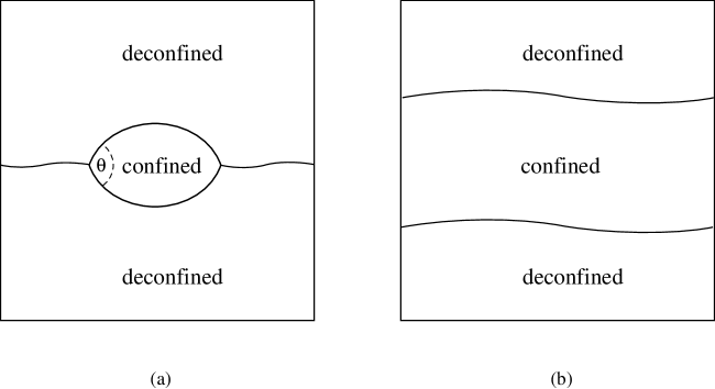
Figure 2: Incomplete versus complete wetting. (a) For $\alpha_{dd}<2\alpha_{cd}$ one has incomplete wetting with $\theta\neq 0$. Then the confined phase forms a lens shaped droplet at the deconfined-deconfined domain wall. (b) Complete wetting corresponds to $\alpha_{dd}=2\alpha_{cd}$. Then $\theta=0$, and the confined phase forms a film that splits the deconfined-deconfined domain wall into two confined-deconfined interfaces.

This equation for $\theta$ follows from the forces at the corner of the lens being in equilibrium. In condensed matter physics the inequality

$$\alpha_{dd}\leq 2\alpha_{cd},$$ (43)

was derived by Widom $\!{}^{{\bf?}}$. It follows from thermodynamic stability because a hypothetical deconfined-deconfined domain wall with $\alpha_{dd}>2\alpha_{cd}$ would simply split into two confined-deconfined interfaces. If $\alpha_{dd}<2\alpha_{cd}$ the confined phase forms droplets at a deconfined-deconfined domain wall. In condensed matter physics this phenomenon is known as incomplete wetting. For $\alpha_{dd}=2\alpha_{cd}$, on the other hand, $\theta=0$ and the lens shaped droplet degenerates to an infinite film, as shown in figure 2b. When such a film is formed, this is called complete wetting.

Complete wetting is a universal phenomenon of interfaces characterized by several critical exponents. For example, the width $r$ of the complete wetting layer diverges as

$$r\propto(T-T_{c})^{-\psi},$$ (44)

where $T-T_{c}$ measures the deviation from the point of phase coexistence and $\psi$ is a critical exponent. The value of $\psi$ depends on the range of the interactions between the two interfaces that enclose the complete wetting layer. In $SU(3)$ Yang-Mills theory the interactions between the interfaces are short-ranged and the interaction energy per unit area is given by $\gamma\exp(-r/r_{0})$. In addition, above $T_{c}$ the confined phase that forms the wetting layer has a slightly larger bulk free energy than the deconfined phases. Close to $T_{c}$, the additional bulk free energy per unit area for a wetting layer of width $r$ is given by $\delta(T-T_{c})r$. Hence, the total free energy per unit area of the two interface system relative to the free energy of two infinitely separated interfaces at $T_{c}$ is given by

$$\alpha_{dd}(T)-2\alpha_{cd}(T_{c})=\gamma\exp(-r/r_{0})+\delta(T-T_{c})r.$$ (45)

Minimizing the free energy with respect to $r$, one finds the equilibrium width

$$r=-r_{0}\log\frac{\delta r_{0}}{\gamma}(T-T_{c}),$$ (46)

such that $\psi=0$. Inserting the equilibrium value of $r$ one finds

$$\alpha_{dd}(T)-2\alpha_{cd}(T_{c})=\delta r_{0}(T-T_{c})[1-\log\frac{\delta r_{0}}{\gamma}(T-T_{c})].$$ (47)

This is consistent with the critical behavior in the ${\sf Z\!\!\!Z}(3)_{c}$ symmetric $\Phi^{4}$ theory $\!{}^{{\bf?}}$. As we will see later, the same critical exponents follow for the high-temperature deconfinement transition in the supersymmetric case.

The universal aspects of the dynamics of confined-deconfined interfaces and deconfined-deconfined domain walls in $SU(3)$ Yang-Mills theory can be investigated using the effective action for the Polyakov loop of eq.(26) $\!{}^{{\bf?}}$. The corresponding potential takes the form $V(\Phi)=a|\Phi|^{2}+b\Phi_{1}(3\Phi_{2}^{2}-\Phi_{1}^{2})+c|\Phi|^{4}$ of eq.(28). The deconfinement phase transition occurs at $b^{2}=4ac$ because then the confined phase minimum at $\Phi^{(4)}=0$ is degenerate with the deconfined phase minimum at $\Phi^{(1)}=\Phi_{0}$ and its ${\sf Z\!\!\!Z}(3)_{c}$ copies at $\Phi^{(2)}$ and $\Phi^{(3)}$. The profile $\Phi(\vec{x})=\Phi(z)$ of a planar interface perpendicular to the $z$-direction follows from the solution of the corresponding classical equations of motion

$$\frac{d^{2}\Phi_{1}}{dz^{2}}=\frac{\partial V}{\partial\Phi_{1}}=2a\Phi_{1}+3b(\Phi_{2}^{2}-\Phi_{1}^{2})+4c\Phi_{1}(\Phi_{1}^{2}+\Phi_{2}^{2}),$$

$$\frac{d^{2}\Phi_{2}}{dz^{2}}=\frac{\partial V}{\partial\Phi_{2}}=2a\Phi_{2}+6b\Phi_{1}\Phi_{2}+4c\Phi_{2}(\Phi_{1}^{2}+\Phi_{2}^{2}).$$ (48)

The solution for a confined-deconfined interface interpolating between the confined phase at negative $z$ and the deconfined phase $\Phi^{(1)}$ at positive $z$ takes the form

$$\Phi_{1}(z)=\frac{1}{2}\Phi_{0}[1+\tanh(\mu z)],\ \Phi_{2}(z)=0.$$ (49)

Here $\mu=b/\sqrt{8c}$ determines the width of the interface. The confined-deconfined interface tension $\alpha_{cd}$ is given by

$$\beta\alpha_{cd}=\int_{-\infty}^{\infty}dz\ [\frac{1}{2}\partial_{i}\Phi^{*}\partial_{i}\Phi+V(\Phi)]=2\int_{-\infty}^{\infty}dz\ V(\Phi)=\frac{\mu\Phi_{0}^{2}}{3}.$$ (50)

The interface profile, its width, as well as its tension are non-universal properties that are quantitatively different in the simple effective $\Phi^{4}$ theory and in $SU(3)$ Yang-Mills theory.

Still, there are universal properties related to the phenomenon of complete wetting. To investigate this, we now consider the profile of a deconfined-deconfined domain wall that interpolates between the deconfined phases $\Phi^{(2)}$ and $\Phi^{(3)}$. The domain wall profile is a solution of eq.(3.2) with the condition that $\Phi$ approaches $\Phi^{(2)}$ at $z=\infty$ and $\Phi^{(3)}$ at $z=-\infty$. A typical solution deep in the deconfined phase is illustrated in fig.3. There is a sharp transition from one deconfined phase to the other. Figure 4 shows the domain wall profile very close to the deconfinement phase transition. In this temperature region the deconfined-deconfined domain wall splits into a pair of confined-deconfined interfaces that enclose a complete wetting layer of confined phase.

Figure 3: Profile of a deconfined-deconfined domain wall in $SU(3)$ Yang-Mills theory deep in the deconfined phase.

Figure 4: Profile of a deconfined-deconfined domain wall in $SU(3)$ Yang-Mills theory close to the phase transition where the wall splits into two confined-deconfined interfaces with a complete wetting layer of confined phase between them.

Very close to the phase transition one can even construct an analytic solution of the completely wet deconfined-deconfined domain wall by combining two solutions for confined-deconfined interfaces

$$\Phi_{1}(z) = -\frac{1}{4}\Phi_{0}[2+\tanh\mu(z-z_{0})-\tanh\mu(z+z_{0})],$$

$$\Phi_{2}(z) = \frac{\sqrt{3}}{4}\Phi_{0}[\tanh\mu(z-z_{0})+\tanh\mu(z+z_{0})].$$ (51)

The interface separation and hence the width of the confined complete wetting layer is given by

$$r=2z_{0}=-\frac{1}{4\mu}\log(\frac{1}{2}-\frac{2ac}{b^{2}}).$$ (52)

Since the phase transition corresponds to $b^{2}=4ac$, the width of the wetting layer diverges logarithmically at $T_{c}$. This is consistent with the critical exponent $\psi=0$ as expected for interfaces with short-range interactions. The interface tension of the deconfined-deconfined domain wall is given by

$$\beta\alpha_{dd}=\mu\Phi_{0}^{2}[\frac{2}{3}-2(1-\frac{4ac}{b^{2}})].$$ (53)

Hence, consistent with the leading $(T-T_{c})$ dependence in eq.(47), one obtains

$$\beta(2\alpha_{cd}-\alpha_{dd})=2\mu\Phi_{0}^{2}(1-\frac{4ac}{b^{2}}).$$ (54)

3.3 Strings Ending on Walls in Supersymmetric Yang-Mills Theory

Witten has argued that color flux strings in supersymmetric Yang-Mills theory can end on domain walls $\!{}^{{\bf?}}$. This effect follows from a calculation in M-theory, where the domain wall is represented by a D-brane on which strings can end. In supersymmetric Yang-Mills theory a ${\sf Z\!\!\!Z}(3)_{\chi}$ chiral symmetry — an unbroken remnant of the anomalous $U(1)_{R}$ symmetry — is spontaneously broken at low temperatures by a non-zero value of the gluino condensate $\chi$. As a consequence, there are three distinct confined phases, characterized by three different values of $\chi$ which are related by ${\sf Z\!\!\!Z}(3)_{\chi}$ transformations. Regions of space filled with different confined phases are separated by confined-confined domain walls. The properties of domain walls in supersymmetric theories have been investigated in great detail by Shifman and collaborators $\!{}^{{\bf?},{\bf?}}$ and also by Carroll, Hellerman and Trodden $\!{}^{{\bf?}}$. Often, topological defects which result from spontaneous symmetry breaking have the phase of unbroken symmetry at their cores. For example, magnetic monopoles or cosmic strings have symmetric vacuum at their centers. Here we construct an effective theory for the Polyakov loop and the gluino condensate in which ${\sf Z\!\!\!Z}(3)_{\chi}$ restoration implies the breaking of the ${\sf Z\!\!\!Z}(3)_{c}$ center symmetry. Then the high-temperature deconfined phase appears at the center of the domain wall forming a complete wetting layer. As a consequence, the Polyakov loop has a non-zero expectation value there and thus a static quark has a finite free energy close to the wall so that its string can end there. In supersymmetric Yang-Mills theory strings can end on confined-confined domain walls because they can transport color flux to infinity at a finite free energy cost. A similar scenario involving a non-Abelian Coulomb phase has been discussed at zero temperature $\!{}^{{\bf?}}$.

In supersymmetric $SU(3)$ Yang-Mills theory the ${\sf Z\!\!\!Z}(3)_{\chi}$ chiral symmetry is spontaneously broken in the confined phase. The corresponding order parameter is the complex valued gluino condensate $\chi=\chi_{1}+i\chi_{2}$. Under chiral transformations $z\in{\sf Z\!\!\!Z}(3)_{\chi}$ the gluino condensate transforms into $\chi^{\prime}=\chi z$ and under charge conjugation it gets replaced by its complex conjugate. At high temperatures one expects chiral symmetry to be restored and — as in the non-supersymmetric theory — the ${\sf Z\!\!\!Z}(3)_{c}$ center symmetry to be spontaneously broken due to deconfinement. Consequently, the effective action describing the interface dynamics now depends on both order parameters $\Phi$ and $\chi$ and

$$S[\Phi,\chi]=\int d^{3}x\ [\frac{1}{2}\partial_{i}\Phi^{*}\partial_{i}\Phi+\frac{1}{2}\partial_{i}\chi^{*}\partial_{i}\chi+V(\Phi,\chi)].$$ (55)

The most general quartic potential consistent with ${\sf Z\!\!\!Z}(3)_{c}$, ${\sf Z\!\!\!Z}(3)_{\chi}$ and charge conjugation symmetry now takes the form

$$V(\Phi,\chi) = a|\Phi|^{2}+b\Phi_{1}(3\Phi_{2}^{2}-\Phi_{1}^{2})+c|\Phi|^{4}$$ (56)

$$+ d|\chi|^{2}+e\chi_{1}(3\chi_{2}^{2}-\chi_{1}^{2})+f|\chi|^{4}+g|\Phi|^{2}|\chi|^{2}.$$

Assuming that deconfinement and chiral symmetry restoration occur at the same temperature and that the phase transition is first order, three chirally broken confined phases coexist with three distinct chirally symmetric deconfined phases. The three deconfined phases have $\Phi^{(1)}=\Phi_{0}$, $\Phi^{(2)}=(-1/2+i\sqrt{3}/2)\Phi_{0}$ and $\Phi^{(3)}=(-1/2-i\sqrt{3}/2)\Phi_{0}$ and $\chi^{(1)}=\chi^{(2)}=\chi^{(3)}=0$, while the three confined phases are characterized by $\Phi^{(4)}=\Phi^{(5)}=\Phi^{(6)}=0$ and $\chi^{(4)}=\chi_{0}\in{\sf I\!\!R}$, $\chi^{(5)}=(-1/2+i\sqrt{3}/2)\chi_{0}$ and $\chi^{(6)}=(-1/2-i\sqrt{3}/2)\chi_{0}$. The phase transition temperature corresponds to a choice of parameters $a,b,...,g$ such that all six phases $\Phi^{(n)}$, $\chi^{(n)}$ represent degenerate absolute minima of $V(\Phi,\chi)$.

We now look for solutions of the classical equations of motion, representing planar domain walls, i.e. $\Phi(\vec{x})=\Phi(z)$, $\chi(\vec{x})=\chi(z)$, where $z$ again is the coordinate perpendicular to the wall. The equations of motion then take the form

$$\frac{d^{2}\Phi_{i}}{dz^{2}}=\frac{\partial V}{\partial\Phi_{i}},\ \frac{d^{2}\chi_{i}}{dz^{2}}=\frac{\partial V}{\partial\chi_{i}}.$$ (57)

Figure 5: Profile of a confined-confined domain wall in supersymmetric $SU(3)$ Yang-Mills theory deep in the confined phase. Note that $\Phi_{1}(0)\neq 0$, i.e. the center of the wall has properties of the deconfined phase.

Figure 6: Profile of a confined-confined domain wall in supersymmetric $SU(3)$ Yang-Mills theory close to the phase transition. In this region the wall splits into two confined-deconfined interfaces with a complete wetting layer of deconfined phase between them.

Figure 5 shows a numerical solution of these equations for a domain wall separating two confined phases of type $c^{(5)}$ and $c^{(6)}$, i.e. with boundary conditions $\Phi(\infty)=\Phi^{(5)}$, $\chi(\infty)=\chi^{(5)}$ and $\Phi(-\infty)=\Phi^{(6)}$, $\chi(-\infty)=\chi^{(6)}$. Figure 5 corresponds to a temperature deep in the confined phase. Still, at the domain wall the Polyakov loop is non-zero, i.e. the center of the domain wall shows characteristic features of the deconfined phase. Figure 6 corresponds to a temperature very close to the phase transition. Then the confined-confined domain wall splits into two confined-deconfined interfaces and the deconfined phase forms a complete wetting layer between them. The solutions of figure 5 have deconfined phase of type $d^{(1)}$ at their centers. Due to the ${\sf Z\!\!\!Z}(3)_{c}$ symmetry, there are related solutions with deconfined phase of types $d^{(2)}$ and $d^{(3)}$.

For the special values $d=a=0$, $e=b$, $f=c$, $g=2c$ one can find an analytic solution for a confined-deconfined interface. Combining two of these solutions to a confined-confined domain wall, one obtains

$$\Phi_{1}(z) = -\frac{1}{2}\Phi_{0}[\tanh\mu(z-z_{0})-\tanh\mu(z+z_{0})],\ \Phi_{2}(z)=0,$$

$$\chi_{1}(z) = -\frac{1}{4}\chi_{0}[2+\tanh\mu(z-z_{0})-\tanh\mu(z+z_{0})],$$

$$\chi_{2}(z) = \frac{\sqrt{3}}{4}\chi_{0}[\tanh\mu(z-z_{0})+\tanh\mu(z+z_{0})],$$ (58)

where $\Phi_{0}=\chi_{0}=3b/4c$ and $\mu=3b/4\sqrt{c}$. The critical temperature corresponds to $e^{4}/f^{3}=b^{4}/c^{3}$. Near criticality, where $\Delta=e^{4}/f^{3}-b^{4}/c^{3}$ is small, the above solution is valid up to order $\Delta^{1/2}$, while now $e=b$ and $f=c$ are satisfied to order $\Delta$. The width of the deconfined complete wetting layer,

$$r=2z_{0}=-\frac{1}{2\mu}\log\Delta+C,$$ (59)

where $C$ is a constant, grows logarithmically as we approach the phase transition temperature. This is the expected critical behavior for interfaces with short-range interactions, which again implies the critical exponent $\psi=0$.

Now we wish to explain why the appearance of the deconfined phase at the center of the domain wall allows a QCD string to end there. We recall that an expectation value $\langle\Phi\rangle\neq 0$ implies that the free energy of a static quark is finite. Indeed, the solution of figure 5 containing deconfined phase of type $d^{(1)}$ has $\Phi_{1}(0)\neq 0$ so that a static quark located at the center of the wall has finite free energy. As one moves away from the wall, the Polyakov loop decreases as

$$\Phi_{1}(z)\propto\exp(-\beta F(z))\propto\exp(-z\sqrt{2a+2g\chi_{0}^{2}}).$$ (60)

Consequently, as the static quark is displaced from the wall, its free energy $F(z)$ increases linearly with the distance $z$ from the center, i.e. the quark is confined to the wall. The string emanating from the static quark ends on the wall and has a tension

$$\sigma=\lim_{z\rightarrow\infty}\frac{F(z)}{z}=\frac{1}{\beta}\sqrt{2a+2g\chi_{0}^{2}}.$$ (61)

Still, there are the other domain wall solutions (related to the one from above by ${\sf Z\!\!\!Z}(3)_{c}$ transformations), which contain deconfined phase of types $d^{(2)}$ and $d^{(3)}$. One could argue that, after path integration over all domain wall configurations, one obtains $\langle\Phi\rangle=0$. However, this is not true. In fact, the wetting layer at the center of a confined-confined domain wall is described by a two-dimensional field theory with a spontaneously broken ${\sf Z\!\!\!Z}(3)_{c}$ symmetry. Consequently, deconfined phase of one definite type spontaneously appears at the domain wall.

4 Paradoxical “Confinement” in the Deconfined Phase

We now want to study some subtle effects related to the spontaneous breakdown of the center symmetry at high temperatures. Whenever a global symmetry gets spontaneously broken, the system becomes very sensitive to the spatial boundary conditions. To expose this sensitivity explicitly, it is often very instructive to work in a finite spatial volume. This is much better than working in an infinite volume with unspecified boundary conditions, which tends to obscure the physics in the infrared. Instead, by consistently working in a finite volume, we learn how the infinite volume limit can be approached in a meaningful way.

4.1 Periodic Versus C-Periodic Spatial Boundary Conditions

Most numerical studies of lattice gauge theories use periodic spatial boundary conditions,

$$A_{\mu}(\vec{x}+L_{i}\vec{e}_{i},x_{4})=A_{\mu}(\vec{x},x_{4}).$$ (62)

Here $L_{i}$ is the size of a 3-dimensional torus in the $i$-direction and $\vec{e}_{i}$ is the unit-vector pointing in that direction. However, periodic boundary conditions are not the most useful ones for studying a single Polyakov loop. As we have seen, a Polyakov loop represents a single static quark that transforms non-trivially under the center of the gauge group. Indeed, the test quark carries a non-zero ${\sf Z\!\!\!Z}(N)_{c}$ charge. For topological reasons, a single charged particle cannot exist in a periodic volume. The flux emanating from the charge cannot escape to infinity and consequently the Gauss law demands that it must end in a compensating anti-charge $\!{}^{{\bf?}}$. As a whole, a periodic system is always neutral.

Here we consider periodic boundary conditions in the $x$ and $y$-directions and $C$-periodic boundary conditions in the $z$-direction $\!{}^{{\bf?},{\bf?}}$. When a $C$-periodic field is shifted by $L_{z}$, it is replaced by its charge conjugate, i.e. for $C$-periodic gluons

$$A_{\mu}(\vec{x}+L_{z}\vec{e}_{z},t)=\ ^{C}\!A_{\mu}(\vec{x},t)=A_{\mu}(\vec{x},t)^{*}.$$ (63)

In a $C$-periodic volume, a single quark can exist, because now its center electric flux can escape to its charge conjugate partner on the other side of the boundary. Note that the system is still translationally invariant. The allowed gauge transformations, as well as the Polyakov loop, also satisfy $C$-periodicity

$$g(\vec{x}+L_{z}\vec{e}_{z},t)=g(\vec{x},t)^{*},\ \Phi(\vec{x}+L_{z}\vec{e}_{z})=\Phi(\vec{x})^{*}.$$ (64)

As a consequence of the boundary conditions, the ${\sf Z\!\!\!Z}(3)_{c}$ center symmetry is now explicitly broken $\!{}^{{\bf?}}$. If one again considers a transformation $g(\vec{x},t+\beta)=zg(\vec{x},t)$, which is periodic, up to a center element $z\in{\sf Z\!\!\!Z}(3)_{c}$, in the Euclidean time direction, one finds

$$g(\vec{x},t)^{*}=g(\vec{x},t+\beta)^{*}z=g(\vec{x}+L_{z}\vec{e}_{z},t+\beta)z=g(\vec{x}+L_{z}\vec{e}_{z},t)z^{2}=g(\vec{x},t)^{*}z^{2}.$$ (65)

Consistency requires $z^{2}=1$ and hence $z=1$ (because $z\in{\sf Z\!\!\!Z}(3)_{c}$). Of course, in the infinite volume limit, the explicit ${\sf Z\!\!\!Z}(3)_{c}$ symmetry breaking due to the spatial boundary conditions disappears. With $C$-periodic boundary conditions, $\langle\Phi\rangle$ is always non-zero in a finite volume. In the confined phase $\langle\Phi\rangle$ goes to zero in the infinite volume limit, while it remains finite in the high-temperature deconfined phase. $C$-periodic boundary conditions are well-suited for studying the free energy of single quarks, while with periodic boundary conditions a single quark cannot even exist.

4.2 Static Quarks in $C$-periodic Cylinders below and above $T_{c}$

First, we consider the system in the confined phase at temperatures $T<T_{c}$ in a cylindrical volume with cross section $A=L_{x}L_{y}$ and length $L_{z}\gg L_{x},L_{y}$. Diagrammatically, the partition function is

$$Z=\begin{picture}(90.0,15.0)\put(0.0,-4.0){\line(1,0){90.0}} \put(0.0,11.0){\line(1,0){90.0}} \put(0.0,-4.0){\line(0,1){15.0}} \put(90.0,-4.0){\line(0,1){15.0}} \put(43.0,0.0){$c$} \end{picture}\ =\exp(-\beta f_{c}AL_{z}),$$ (66)

where $f_{c}$ is the temperature-dependent free energy density in the confined phase. The expectation value of the Polyakov loop (times $Z$), on the other hand, is given by

$$Z\langle\Phi\rangle=\begin{picture}(90.0,15.0)\put(0.0,-4.0){\line(1,0){90.0}} \put(0.0,11.0){\line(1,0){90.0}} \put(0.0,-4.0){\line(0,1){15.0}} \put(90.0,-4.0){\line(0,1){15.0}} \put(43.0,0.0){$c$} \put(0.0,3.5){\line(1,0){38.0}} \put(52.0,3.5){\line(1,0){38.0}} \end{picture}\ =\exp(-\beta f_{c}AL_{z})\Sigma_{0}\exp(-\beta\sigma L_{z}),$$ (67)

where $\sigma$ is the string tension, which is again temperature-dependent. The confining string (denoted by the additional line in the diagram) connects the static quark with its anti-quark partner on the other side of the $C$-periodic boundary. Hence, the free energy of the quark is given by

$$F=-\frac{1}{\beta}\log\Sigma_{0}+\sigma L_{z}.$$ (68)

The free energy diverges as $L_{z}\rightarrow\infty$, indicating that the quark is confined.

Now let us consider the deconfined phase at temperatures $T>T_{c}$, where three distinct deconfined phases coexist. In a cylindrical volume, a typical configuration consists of several bulk phases, aligned along the $z$-direction, separated by deconfined-deconfined domain walls. The domain walls cost free energy $F$ proportional to their area $A$, such that their tension is given by $\alpha_{dd}=F/A$. What matters in the following is the cylindrical shape, not the magnitude of the volume. In fact, the cylinders can be of macroscopic size. The expectation value of the Polyakov loop in a cylindrical volume can be calculated from a dilute gas of domain walls $\!{}^{{\bf?}}$. The domain wall expansion of the partition function can be viewed as

$$Z=\begin{picture}(90.0,15.0)\put(0.0,-4.0){\line(1,0){90.0}} \put(0.0,11.0){\line(1,0){90.0}} \put(0.0,-4.0){\line(0,1){15.0}} \put(90.0,-4.0){\line(0,1){15.0}} \put(40.0,0.0){$d^{(1)}$} \end{picture}\ +\ \begin{picture}(90.0,15.0)\put(0.0,-4.0){\line(1,0){90.0}} \put(0.0,11.0){\line(1,0){90.0}} \put(0.0,-4.0){\line(0,1){15.0}} \put(90.0,-4.0){\line(0,1){15.0}} \put(45.0,-4.0){\line(0,1){15.0}} \put(18.0,0.0){$d^{(2)}$} \put(63.0,0.0){$d^{(3)}$} \end{picture}\ +\ \begin{picture}(90.0,15.0)\put(0.0,-4.0){\line(1,0){90.0}} \put(0.0,11.0){\line(1,0){90.0}} \put(0.0,-4.0){\line(0,1){15.0}} \put(90.0,-4.0){\line(0,1){15.0}} \put(45.0,-4.0){\line(0,1){15.0}} \put(18.0,0.0){$d^{(3)}$} \put(63.0,0.0){$d^{(2)}$} \end{picture}\ +...$$ (69)

The first term has no domain walls and thus the whole cylinder is filled with deconfined phase $d^{(1)}$ only. An entire volume filled with either phase $d^{(2)}$ or $d^{(3)}$ would not satisfy the boundary conditions. The second and third terms have one domain wall separating phases $d^{(2)}$ and $d^{(3)}$. Here, $C$-periodic boundary conditions exclude phase $d^{(1)}$. The sum of the diagrammatic terms is given by

$$Z = \exp(-\beta f_{d}AL_{z})$$ (70)

$$+ 2\int_{0}^{L_{z}}dz\ \exp(-\beta f_{d}Az)\gamma\exp(-\beta\alpha_{dd}A)\exp(-\beta f_{d}A(L_{z}-z))+...$$

$$= \exp(-\beta f_{d}AL_{z})[1+2\gamma\exp(-\beta\alpha_{dd}A)L_{z}+...].$$

The first term is the Boltzmann weight of deconfined phase of volume $AL_{z}$ with a free energy density $f_{d}$. The second term contains two of these bulk Boltzmann factors separated by a domain wall contribution $\gamma\exp(-\beta\alpha_{dd}A)$, where $\gamma$ is a factor resulting from capillary wave fluctuations of the domain wall. In the above expression, we have integrated over all possible locations $z$ of the domain wall. It is straightforward to sum the domain wall expansion to all orders, giving

$$Z=\exp(-\beta f_{d}AL_{z}+2\gamma\exp(-\beta\alpha_{dd}A)L_{z}).$$ (71)

In exactly the same way one obtains

$$\langle\Phi\rangle=\Phi_{0}\exp(-3\gamma\exp(-\beta\alpha_{dd}A)L_{z}).$$ (72)

The free energy of a static quark in a $C$-periodic cylinder is therefore given by

$$F=-\frac{1}{\beta}\log\Phi_{0}+\frac{3\gamma}{\beta}\exp(-\beta\alpha_{dd}A)L_{z}.$$ (73)

This result is counter intuitive. Although we are in the deconfined phase, the quark’s free energy diverges in the limit $L_{z}\rightarrow\infty$, as long as the cross section $A$ of the cylinder remains fixed. This is the behavior one typically associates with confinement. In fact,

$$\sigma^{\prime}=\frac{3\gamma}{\beta}\exp(-\beta\alpha_{dd}A)$$ (74)

plays the role of a “string tension”, even though there is no physical string that connects the quark with its anti-quark partner on the other side of the $C$-periodic boundary. “Confinement” in $C$-periodic cylinders arises because disorder due to many differently oriented deconfined phases destroys the correlations of center electric flux between quark and anti-quark.

Of course, this paradoxical confinement mechanism is due to the cylindrical geometry and the specific boundary conditions. Had we chosen $C$-periodic boundary conditions in all directions, the deconfined phases $d^{(2)}$ and $d^{(3)}$ would be exponentially suppressed, so that the entire volume would be filled with phase $d^{(1)}$ only. In that case, the free energy of a static quark is $F=-(1/\beta)\log\Phi_{0}$, which does not diverge in the infinite volume limit, as expected. Had we worked in a cubic volume, a typical configuration would have no domain walls, the whole volume would be filled with deconfined phase $d^{(1)}$ and again the free energy of a static quark would be $F=-(1/\beta)\log\Phi_{0}$. Finally, note that, in a cylindrical volume, even the static Coulomb potential is linearly rising with a “string tension” $e^{2}/A$. Due to Debye screening, this trivial confinement effect is absent in the gluon plasma.

The observed paradoxical confinement implies that deconfined-deconfined domain walls are more than just Euclidean field configurations. In fact, they can lead to a divergence of the free energy of a static quark and thus they have physically observable consequences even in Minkowski space-time. Of course, the issue is rather academic. First of all, the existence of three distinct deconfined phases relies on the ${\sf Z\!\!\!Z}(3)_{c}$ symmetry, which only exists in a pure gluon system — not in the real world with light dynamical quarks. Second, the effect is due to the cylindrical geometry and our choice of boundary conditions. Even though it is not very realistic, this set-up describes a perfectly well-defined Gedanken experiment, demonstrating the physical reality of deconfined-deconfined domain walls.

5 Conclusions

Thanks to the efforts of numerous people, the role of the center symmetry for the confinement and deconfinement of static quarks is by now very well understood and is more or less a closed subject. In this article we have concentrated on those aspects of the problem that can be easily explained using simple analytic calculations in continuum field theory. However, we again want to emphasize the very important role that lattice field theory, in particular, numerical simulation of $SU(2)$ and $SU(3)$ Yang-Mills theory has played in understanding the dynamical role of the center symmetry. It is fair to say that lattice gauge theory has led to a reliable high-precision numerical solution of Yang-Mills theories. Due to severe numerical problems in dealing with fermionic fields, this can presently not be said about full QCD including dynamical quarks. Still, continuous progress is being made in applying lattice methods and it is to be expected that an accurate numerical solution of QCD will eventually be obtained. In contrast to Yang-Mills theory, the center symmetry plays a minor role in full QCD because it is explicitly broken in the presence of quarks. However, along the way, other theories — for example, supersymmetric Yang-Mills theories — can be solved with lattice field theory methods as well. At that point the center symmetry may become an interesting research topic again. In any case, we hope that we have convinced the reader that — thanks to the center symmetry — a world without quarks would not be quite as boring as one might have naively expected.

References

References

- [1] G. ’t Hooft, Nucl. Phys. B138, 1 (1978); Nucl. Phys. B153, 141 (1979).
- [2] A. M. Polyakov, Phys. Lett. B72, 477 (1978).
- [3] L. Susskind, Phys. Rev. D20, 2610 (1979).
- [4] L. D. McLerran and B. Svetitsky, Phys. Rev. D24, 450 (1981).
- [5] B. Svetitsky and L. G. Yaffe, Nucl. Phys. B210, 423 (1982).
-
[6]
L. D. McLerran and B. Svetitsky, Phys. Lett. B98, 195 (1981);
J. Kuti, J. Polonyi and K. Szlachanyi, Phys. Lett. B98, 199 (1981);
J. Engels, F. Karsch, H. Satz and I. Montvay, Phys. Lett. B101, 89 (1981);
R. V. Gavai, Nucl. Phys. B215, 458 (1983);
R. V. Gavai, F. Karsch and H. Satz, Nucl. Phys. B220, 223 (1983). -
[7]
J. Engels, J. Fingberg and M. Weber, Nucl. Phys. B332, 737 (1990);
J. Engels, J. Fingberg and D. E. Miller, Nucl. Phys. B387, 501 (1992). -
[8]
J. Fingberg, U. M. Heller and F. Karsch, Nucl. Phys. B392, 493 (1993);
T. DeGrand, A. Hasenfratz and D. Zhu, Nucl. Phys. B478, 349 (1996). - [9] F. Y. Wu, Rev. Mod. Phys. 54, 235 (1982).
-
[10]
S. J. Knak Jensen and O. G. Mouritsen, Phys. Rev. Lett. 43, 1736 (1979);
H. W. J. Blöte and R. H. Swendsen, Phys. Rev. Lett. 43, 799 (1979);
H. J. Herrmann, Z. Phys. B35, 171 (1979);
F. Y. Wu, Rev. Mod. Phys. 54, 235 (1982);
M. Fukugita and M. Okawa, Phys. Rev. Lett. 63, 13 (1989);
R. V. Gavai, A. Irback, B. Petersson and F. Karsch, Nucl. Phys. B (Proc. Suppl.)17, 199 (1990);
A. J. Guttmann and I. G. Enting, Nucl. Phys. B (Proc. Suppl.)17, 328 (1990). - [11] L. G. Yaffe and B. Svetitsky, Phys. Rev. D26, 963 (1982).
-
[12]
T. Celik, J. Engels and H. Satz, Phys. Lett. B125, 411 (1983);
J. Kogut, M. Stone, H. W. Wyld, W. R. Gibbs, J. Shigemitsu, S. H. Shenker and D. K. Sinclair, Phys. Rev. Lett. 50, 393 (1983);
S. A. Gottlieb, J. Kuti, D. Toussaint, A. D. Kennedy, S. Meyer, B. J. Pendleton and R. L. Sugar, Phys. Rev. Lett. 55, 1958 (1985);
F. R. Brown, N. H. Christ, Y. F. Deng, M. S. Gao and T. J. Woch, Phys. Rev. Lett. 61, 2058 (1988);
R. V. Gavai, F. Karsch and B. Petersson, Nucl. Phys. B322, 738 (1989);
M. Fukugita, M. Okawa and A. Ukawa, Phys. Rev. Lett. 63, 1768 (1989);
N. A. Alves, B. A. Berg and S. Sanielevici, Phys. Rev. Lett. 64, 3107 (1990). - [13] T. Bhattacharya, A. Gocksch, C. Korthals Altes and R. D. Pisarski, Phys. Rev. Lett. 66, 998 (1991).
-
[14]
S. Huang, J. Potvin, C. Rebbi and S. Sanielevici,
Phys. Rev. D42, 2864 (1990);
K. Kajantie, L. Karkkainen and K. Rummukainen, Nucl. Phys. B333, 100 (1990); Nucl. Phys. B357, 693 (1991);
R. Brower, S. Huang, J. Potvin, C. Rebbi and J. Ross, Phys. Rev. D46, 4736 (1992);
W. Janke, B. A. Berg and M. Katoot, Nucl. Phys. B382, 649 (1992);
B. Grossmann, M. L. Laursen, T. Trappenberg and U.-J. Wiese, Nucl. Phys. B396, 584 (1993); Phys. Lett. B293, 175 (1992);
B. Grossmann and M. L. Laursen, Nucl. Phys. B408, 637 (1993);
Y. Iwasaki, K. Kanaya, L. Karkkainen, K. Rummukainen and T. Yoshie, Phys. Rev. D49, 1994 (3540);
Y. Aoki and K. Kanaya, Phys. Rev. D50, 6921 (1994). - [15] J. Ignatius, K. Kajantie and K. Rummukainen, Phys. Rev. Lett. 68, 737 (1992).
- [16] N. Weiss, Phys. Rev. D24, 475 (1981).
- [17] Z. Frei and A. Patkós, Phys. Lett. B229, 102 (1989).
- [18] T. Trappenberg and U.-J. Wiese, Nucl. Phys. B372, 703 (1992).
- [19] A. Campos, K. Holland and U.-J. Wiese, Phys. Rev. Lett. 81, 2420 (1998); Phys. Lett. B443, 338 (1998).
- [20] E. Witten, Nucl. Phys. B507, 658 (1997).
-
[21]
V. M. Belyaev, I. I. Kogan, G. W. Semenoff and N. Weiss,
Phys. Lett. B277, 331 (1992) ;
A. V. Smilga, Ann. Phys. 234, 1 (1994);
T. H. Hansson, H. B. Nielsen and I. Zahed, Nucl. Phys. B451, 162 (1995). - [22] E. Hilf and L. Polley, Phys. Lett. B131, 412 (1983).
- [23] L. Polley and U.-J. Wiese, Nucl. Phys. B356, 629 (1991).
- [24] A. S. Kronfeld and U.-J. Wiese, Nucl. Phys. B357, 521 (1991).
- [25] U.-J. Wiese, Nucl. Phys. B375, 45 (1992).
-
[26]
K. Holland and U.-J. Wiese, Phys. Lett. B415, 179 (1997);
K. Holland, Phys. Rev. D60, 074022 (1999). - [27] F. Lenz and M. Thies, Ann. Phys. 268, 308 (1998).
- [28] C. Korthals Altes, A. Kovner and M. Stephanov, Phys. Lett. B469, 205 (1999).
-
[29]
T. Blum, J. Hetrick and D. Toussaint, Phys. Rev. Lett. 76, 1019 (1996);
J. Engels, O. Kaczmarek, F. Karsch and E. Laermann, Nucl. Phys. B558, 307 (1999). - [30] M. Alford, S. Chandrasekharan, J. Cox and U.-J. Wiese, in preparation.
- [31] F. Karsch and S. Stickan, hep-lat/0007019.
- [32] B. Widom, J. Chem. Phys. 62, 1332 (1975).
-
[33]
A. Kovner, M. Shifman and A. V. Smilga, Phys. Rev. D56, 7978 (1997);
G. Dvali and M. Shifman, Phys. Lett. B396, 64 (1997);
M. Shifman, M. B. Voloshin, Phys. Rev. D57, 2590 (1998);
A. V. Smilga and A. I. Veselov, Nucl. Phys. B515, 163 (1998). - [34] I. I. Kogan, A. Kovner and M. Shifman, Phys. Rev. D57, 5195 (1998).
-
[35]
S. Carroll and M. Trodden, Phys. Rev. D57, 5189 (1998);
S. Carroll, S. Hellerman and M. Trodden, Phys. Rev. D61, 065001 (2000).