BUTP 2000/11
November 2000

QED Corrections to Neutrino
Electron Scattering

M. Passera

Institut für Theoretische Physik, Universität Bern,
Sidlerstrasse 5, CH-3012 Bern, Switzerland

Abstract

We evaluate the $O(\alpha)$ QED corrections to the recoil electron energy spectrum in the process $\nu_{l}+e\rightarrow\nu_{l}+e\;(+\gamma)$, where $(+\gamma)$ indicates the possible emission of a photon and $l=e$, $\mu$ or $\tau$. The soft and hard bremsstrahlung differential cross sections are computed for an arbitrary value of the photon energy threshold. We also study the $O(\alpha)$ QED corrections to the differential cross section with respect to the total combined energy of the recoil electron and a possible accompanying photon. Their difference from the corrections to the electron spectrum is investigated. We discuss the relevance and applicability of both radiative corrections, emphasizing their role in the analysis of precise solar neutrino electron scattering experiments.

1 Introduction

The QED corrections to the scattering process $\nu_{e}+e\rightarrow\nu_{e}+e$ were studied long ago by Lee and Sirlin using the effective four–fermion V$-$A Lagrangian [1], and shortly afterwards Ram [2] extended their calculations by including hard photon emission. A few years later, ’t Hooft computed the lowest order prediction to this differential cross section in the Standard Model (SM) [3]. Since then, the radiative corrections to this process, which plays a fundamental role in the study of electroweak interactions, have been investigated by many authors, focusing on various aspects of the problem [4, 5, 6, 7, 8, 9, 10, 11, 12, 13, 14].

’t Hooft’s early SM predictions for $\nu$–$e$ scattering were used by Bahcall to examine the total cross section, energy spectrum and angular distribution of recoil electrons resulting from the scattering with solar neutrinos [15]. More recently, Bahcall, Kamionkowski and Sirlin performed a detailed investigation of the radiative corrections to these recoil electron spectra and total cross sections [16]. Their results show the importance of these corrections for the analysis of precise solar $\nu$–$e$ scattering experiments, particularly of those measuring the higher energy neutrinos that originate from $\!\!\!\!\phantom{A}{}^{8}$B decay.

In this paper we study the $O(\alpha)$ QED corrections to neutrino electron scattering in the SM, with contributions involving either neutral currents (as in the $\nu_{\mu,\tau}+e\rightarrow\nu_{\mu,\tau}+e$ process) or a combination of neutral and charged currents (as in the $\nu_{e}+e\rightarrow\nu_{e}+e$ process). In this analysis we make the approximation of neglecting terms of $O(q^{2}/M_{\scriptscriptstyle W}^{2})$, where $q^{2}$ is the squared four-momentum transfer and $M_{\scriptscriptstyle W}$ is the $W$ boson mass. Within this approximation, which is excellent for present experiments ($|q^{2}/M_{\scriptscriptstyle W}^{2}|\!\sim\!1$ when the electron recoil energy $\sim 6\times 10^{3}$ TeV!), the SM radiative corrections to these processes can be naturally divided into two classes. The first, which we will call “QED” corrections, consist of the photonic radiative corrections that would occur if the theory were a local four–fermion Fermi theory rather than a gauge theory mediated by vector bosons; the second, which we will refer to as the “electroweak” (EW) corrections, will be the remainder. The EW corrections have been studied by several authors [5, 6, 7, 8, 10, 16] and are not discussed in the present paper. The split–up of the QED corrections is sensible as they form a finite (both infrared and ultraviolet) and gauge–independent subset of diagrams. We refer the reader to ref. [17] for a detailed study of this separation.

The QED radiative corrections are due to both loop diagrams (virtual corrections) and to the bremsstrahlung radiation (real photons) accompanying the scattering process. Of course, only this combination of virtual and real photon corrections is free from infrared divergences. To order $\alpha$, the bremsstrahlung events correspond to the inelastic process $\nu_{l}+e\rightarrow$ $\nu_{l}+e+\gamma$ ($l=e,\mu$ or $\tau$). Experimentally, bremsstrahlung events in which photons are too soft to be detected are counted as contributions to the elastic scattering $\nu_{l}+e\rightarrow$ $\nu_{l}+e$. The cross section for these events should be therefore added to the theoretical prediction of the elastic cross section, thus removing its infrared divergence.

We will divide the bremsstrahlung events into “soft” (hereafter SB) and “hard” (hereafter HB), according to the energy of the photon being respectively lower or higher than some specified threshold $\epsilon$. We should warn the reader that the words “soft” and “hard” may be slightly deceiving. Indeed, if $\epsilon$ is large (small), the SB (HB) cross section will also include events with relatively high (low) energy photons. While calculations of both soft and hard bremsstrahlung are often performed under the assumption that $\epsilon$ is a very small parameter, much smaller than the mass of the electron or its final momentum, we will also discuss results for the case in which $\epsilon$ is an arbitrary parameter constrained only by the kinematics of the process. Indeed, the HB cross section (contrary to the SB one) is by itself, at least in principle, a physically measurable quantity for any kinematically allowed value of this threshold. All calculations have been carried out without neglecting the electron mass.

The paper is organized as follows. In sect. 2 we discuss the lowest order prediction for the neutrino electron differential cross section, together with its soft bremsstrahlung and one–loop QED corrections. The hard bremsstrahlung recoil electron spectrum is examined in sect. 3. In the same section, this contribution is added to the virtual and soft ones to derive the total QED corrections. In sect. 4 we evaluate the spectrum of the total combined energy of the recoil electron and a possible accompanying photon emitted in the scattering process. We summarize our main results in sect. 5, discussing their applicability and emphasizing their role in the analysis of solar neutrino electron scattering experiments.

2 Virtual and Soft Photon Corrections

The SM prediction for the elastic neutrino electron differential cross section is, in lowest–order and neglecting terms of $O(q^{2}/M_{\scriptscriptstyle W}^{2})$ [3],

$$\left[\frac{d\sigma}{dE}\right]_{0}\;=\;\frac{2mG_{\mu}^{2}}{\pi}\left[g_{\scriptscriptstyle L}^{2}+g_{\scriptscriptstyle R}^{2}\left(1-z\right)^{2}-g_{\scriptscriptstyle L}g_{\scriptscriptstyle R}\left(\frac{mz}{\nu}\right)\right],$$ (1)

where $m$ is the electron mass, $G_{\mu}=1.16637(1)\times 10^{-5}\mbox{ GeV}^{-2}$ is the Fermi coupling constant [18], $g_{\scriptscriptstyle L}=\sin^{2}\!\theta_{{\scriptscriptstyle W}}\pm 1/2$ (upper sign for $\nu_{e}$, lower sign for $\nu_{\mu,\tau}$), $g_{\scriptscriptstyle R}=\sin^{2}\!\theta_{{\scriptscriptstyle W}}$ and $\sin\theta_{{\scriptscriptstyle W}}$ is the sine of the weak mixing angle. In this elastic process $E$, the electron recoil energy, ranges from $m$ to $E_{\rm\scriptstyle max}=$ $[m^{2}+(2\nu+m)^{2}]/[2(2\nu+m)]$, $z=(E-m)/\nu$ and $\nu$ is the incident neutrino energy in the frame of reference in which the electron is initially at rest. We will refer to the $L$, $R$ and $LR$ parts of an expression to indicate its terms proportional to $g_{\scriptscriptstyle L}^{2}$, $g_{\scriptscriptstyle R}^{2}$ and $g_{\scriptscriptstyle L}g_{\scriptscriptstyle R}$, respectively. For example, the $R$ part of $\left[d\sigma/dE\right]_{0}$ (eq. (1)) is $(2mG_{\mu}^{2}/\pi)g_{\scriptscriptstyle R}^{2}(1-z)^{2}$.

According to the definition discussed earlier, the one–loop QED corrections to neutrino electron scattering consist of the photonic vertex corrections (together with the diagrams involving the field renormalization of the electrons) computed with the local four–fermion Fermi Lagrangian. These corrections give rise to the following expression for the differential cross section:

$$\left[\frac{d\sigma}{dE}\right]_{\rm Virtual}\;=\;\frac{2mG_{\mu}^{2}}{\pi}\Biggl{[}\frac{\alpha}{\pi}\,\delta(E,\nu)\Biggr{]},$$ (2)

where

$$\delta(E,\nu) = g_{\scriptscriptstyle L}^{2}\;\left\{V_{1}(E)+V_{2}(E)\left[z-1-\frac{mz}{2\nu}\right]\right\}$$ (3)

$$+ g_{\scriptscriptstyle R}^{2}\;\left\{V_{1}(E)\left(1-z\right)^{2}+V_{2}(E)\left[z-1-\frac{mz}{2\nu}\right]\right\}$$

$$- g_{\scriptscriptstyle L}g_{\scriptscriptstyle R}\,\left\{\left[V_{1}(E)-V_{2}(E)\right]\left(\frac{mz}{\nu}\right)+2V_{2}(E)\left[z-1-z^{2}\right]\right\},$$

$$V_{1}(E) = \left(2\ln\!\frac{m}{\lambda}\right)\left[1-\frac{E}{2l}\ln\!\left(\frac{E+l}{E-l}\right)\right]-2-\frac{E}{l}\left[\,\mbox{Li}_{2}\!\left(\frac{l-E+m}{2l}\right)\right.$$ (4)

$$- \left.\mbox{Li}_{2}\!\left(\frac{l+E-m}{2l}\right)\right]+\frac{1}{4l}\left[3E+m-E\ln\!\left(\frac{2E+2m}{m}\right)\right]\ln\!\left(\frac{E+l}{E-l}\right),$$

$$V_{2}(E) = \frac{m}{4l}\ln\!\left(\frac{E+l}{E-l}\right).$$ (5)

$\lambda$ is a small photon mass introduced to regularize the infrared divergence and $l=\sqrt{E^{2}-m^{2}}$ is the three-momentum of the electron. The dilogarithm $\mbox{Li}_{2}(x)$ is defined by

$$\mbox{Li}_{2}(x)=-\int_{0}^{x}\!dt\,\frac{\ln(1-t)}{t}.$$

The $L$ part of eq. (2) (with $g_{\scriptscriptstyle L}=1$) is identical to the formula for the one–loop photonic corrections to the $\nu_{e}+e\rightarrow\nu_{e}+e$ differential cross section computed long ago in the pioneering work of Lee and Sirlin [1] using the effective four–fermion Fermi V$-$A Lagrangian. The analogous formula for the reaction involving an anti–neutrino $\overline{\nu}_{e}$ (rather than a neutrino $\nu_{e}$) can be found in the same article and coincides with the $R$ part of eq. (2) (with $g_{\scriptscriptstyle R}=1$). This identity is simply due to the fact that the cross section for antineutrinos in the local V$-$A theory is the same as that for neutrinos calculated with a V$+$A coupling. On the contrary, the $LR$ part of eq. (2) has clearly no analogue in the V$\pm$A theory, but can be derived very easily once the $L$ and $R$ parts are known.

The $\nu_{e}+e\rightarrow$ $\nu_{e}+e+\gamma$ differential cross section with emission of a soft photon was computed in ref. [1], once again by using the effective four–fermion Fermi V$-$A Lagrangian. It can be identified with the $L$ part (with $g_{\scriptscriptstyle L}=1$) of the soft photon corrections to the tree level result in eq. (1). The $L$, $R$ and $LR$ parts of these corrections (with $g_{\scriptscriptstyle L}=g_{\scriptscriptstyle R}=1$) are however identical, because the whole soft bremsstrahlung cross section is proportional to its lowest–order elastic prediction. We can therefore write the soft photon emission cross section in the following factorized form:

$$\left[\frac{d\sigma}{dE}\right]_{\rm SB}\;=\;\frac{\alpha}{\pi}\;I_{\gamma}(E,\epsilon)\left[\frac{d\sigma}{dE}\right]_{0},$$ (6)

with

$$I_{\gamma}(E,\epsilon) = \left(2\ln\!\frac{\lambda}{\epsilon}\right)\left[1-\frac{E}{2l}\ln\!\left(\frac{E+l}{E-l}\right)\right]+\frac{E}{2l}\left\{\,L\!\left(\frac{E+l}{E-l}\right)-L\!\left(\frac{E-l}{E+l}\right)\right.$$ (7)

$$+ \left.\ln\!\left(\frac{E+l}{E-l}\right)\left[1-2\ln\!\left(\frac{l}{m}\right)\right]\right\}+1-2\ln\!2$$

and

$$L(x)=\int_{0}^{x}\!dt\,\frac{\ln|1-t|}{t}.$$

(For $x\in\mbox{I}\!\mbox{R}$, $L(x)=-\mbox{Re}[\mbox{Li}_{2}(x)]$.) This result is valid under the assumption that $\epsilon$, the maximum soft photon energy, is much smaller than $m$ or the final momentum of the electron. As we mentioned earlier, in the next section we will discuss numerical results for the case in which $\epsilon$ is an arbitrary parameter.

The reader will notice that the sum $[V_{1}(E)+I_{\gamma}(E,\epsilon)]$ does not depend on $\lambda$, the infrared regulator. Indeed, the infrared divergence of the virtual corrections (eq. (2)) is canceled by that arising from the soft photon emission (eq. (6)).

3 Hard Bremsstrahlung and Total QED Corrections to the Final Electron Spectrum

The SM prediction for the differential neutrino electron cross section

$$\nu_{l}+e\rightarrow\nu_{l}+e\;(+\gamma),$$ (8)

where $(+\gamma)$ indicates the possible emission of a photon, can be cast, up to corrections of $O(\alpha)$, in the following form:

$$\left[\frac{d\sigma}{dE}\right]_{\rm SM} = \frac{2mG_{\mu}^{2}}{\pi}\Biggl{\{}g_{\scriptscriptstyle L}^{2}(E)\left[1+\frac{\alpha}{\pi}f_{\scriptscriptstyle L}(E,\nu)\right]+g_{\scriptscriptstyle R}^{2}(E)\left(1-z\right)^{2}\left[1+\frac{\alpha}{\pi}f_{\scriptscriptstyle R}(E,\nu)\right]$$ (9)

$$-g_{\scriptscriptstyle L}(E)g_{\scriptscriptstyle R}(E)\left(\frac{mz}{\nu}\right)\left[1+\frac{\alpha}{\pi}f_{{\scriptscriptstyle L}{\scriptscriptstyle R}}(E,\nu)\right]\Biggr{\}}.$$

(We remind the reader that terms of $O(q^{2}/M_{\scriptscriptstyle W}^{2})$ are neglected throughout this paper.) The deviations of the functions $g_{\scriptscriptstyle L}(E)$ and $g_{\scriptscriptstyle R}(E)$ from the lowest–order values $g_{\scriptscriptstyle L}$ and $g_{\scriptscriptstyle R}$ reflect the effect of the electroweak corrections, which have been studied by several authors [5, 6, 7, 8, 10, 16]. (See ref. [16] for simple numerical results.)

The functions $f_{\scriptscriptstyle X}(E,\nu)$ ($X=L,R$ or $LR$) describe the QED effects (real and virtual photons). For simplicity of notation their $\nu$ dependence will be dropped in the following. Each of these functions is the sum of virtual (V), soft (SB) and hard (HB) corrections,

$$f_{\scriptscriptstyle X}(E)=f_{\scriptscriptstyle X}^{\scriptscriptstyle V}(E)+f_{\scriptscriptstyle X}^{\scriptscriptstyle SB}(E,\epsilon)+f_{\scriptscriptstyle X}^{\scriptscriptstyle HB}(E,\epsilon).$$ (10)

(We remind the reader that we have defined the bremsstrahlung events as “soft” or “hard” according to the energy of the photon being respectively smaller or higher than a specified threshold $\epsilon$.) The analytic expressions for $f_{\scriptscriptstyle X}^{\scriptscriptstyle V}(E)$ and $f_{\scriptscriptstyle X}^{\scriptscriptstyle SB}(E,\epsilon)$ can be immediately read from eqs. (2) and (6) respectively (the latter being valid only in the small $\epsilon$ limit) and their sums, which are infrared–finite, will be denoted by

$$f_{\scriptscriptstyle X}^{\scriptscriptstyle VS}(E,\epsilon)=f_{\scriptscriptstyle X}^{\scriptscriptstyle V}(E)+f_{\scriptscriptstyle X}^{\scriptscriptstyle SB}(E,\epsilon).$$ (11)

Analytic expressions from which one can obtain $f_{\scriptscriptstyle L}^{\scriptscriptstyle HB}(E,\epsilon)$ and $f_{\scriptscriptstyle R}^{\scriptscriptstyle HB}(E,\epsilon)$ were calculated long ago by Ram [2]. Although these results were obtained in the small $\epsilon$ approximation, the formulae are nonetheless long and complicated and we will only plot the results for specific values of $\nu$ and $\epsilon$. The function $f_{{\scriptscriptstyle L}{\scriptscriptstyle R}}^{\scriptscriptstyle HB}(E,\epsilon)$ has not been previously calculated.

We created BC, a combined Mathematica–FORTRAN code to compute the $f_{\scriptscriptstyle X}^{\scriptscriptstyle HB}(E,\epsilon)$ functions for arbitrary positive values of the parameter $\epsilon$ up to the kinematic limit $\nu$ ($\nu$, the incident neutrino energy in the laboratory system, is also the maximum possible energy of the emitted photon). We first computed the transition probability for the bremsstrahlung process, averaged over the initial electron spins and summed over the polarizations of the final electron and photon. We then removed the energy–momentum conserving $\delta$ function in the three–body phase–space integral and specialized the result to the laboratory frame of reference. For a given initial neutrino energy, the five independent variables describing the final state were chosen to be the four angular variables of the final electron and photon, plus the electron recoil energy. In order to compute the HB functions $f_{\scriptscriptstyle X}^{\scriptscriptstyle HB}(E,\epsilon)$ we finally imposed the condition that the photon energy $\omega$ should be larger than the threshold $\epsilon$ (without assuming $\epsilon$ to be small). This constraint required a detailed analysis of the kinematically allowed ranges of variability of the chosen phase–space variables. The last integrations over the angular variables were then performed numerically using the Monte Carlo method [20] and demanding a $0.1\%$ relative accuracy. (Reminding the reader that $X$ indicates $L$, $R$ or $LR$, we note that this uncertainty in the computation of a function $f_{\scriptscriptstyle X}^{\scriptscriptstyle HB}(E,\epsilon)$ produces an extremely tiny relative error $(\alpha/\pi)f_{\scriptscriptstyle X}^{\scriptscriptstyle HB}(E,\epsilon)\times 0.1\%$ in the corresponding $X$ part of the differential cross section in eq. (9). This high level of accuracy was useful for internal numerical checks and for the comparisons, in the small $\epsilon$ limit, with Ram’s results.) All calculations have been carried out without neglecting the electron mass.

In figs. 1 and 2 the functions $f_{\scriptscriptstyle X}^{\scriptscriptstyle HB}(E,\epsilon)$ are respectively plotted for $\nu=0.862\mbox{ MeV}$ and $\nu=10\mbox{ MeV}$, setting the threshold $\epsilon$ to several different values. These two values of $\nu$ were chosen for their relevance in the study of solar neutrinos: $\nu=0.862\mbox{ MeV}$ is the energy of the monochromatic neutrinos produced by electron capture on $\!\!\!\!\phantom{A}{}^{7}$Be in the solar interior, while $\nu=10\mbox{ MeV}$ belongs to the continuous energy spectrum of the solar neutrinos that originate from $\!\!\!\!\phantom{A}{}^{8}$B decay. In the same figures we compared the results of our code BC (solid lines) with the approximate analytic results of Ram (dotted lines). (There are no dotted lines in the $LR$ plots because the function $f_{{\scriptscriptstyle L}{\scriptscriptstyle R}}^{\scriptscriptstyle HB}(E,\epsilon)$ has not been previously calculated.) As we mentioned earlier, Ram’s formulae were computed in the small $\epsilon$ approximation, keeping the logarithmically divergent terms proportional to $\ln(\epsilon/m)$, but neglecting the remaining $\epsilon$–dependent terms. Our results confirm Ram’s ones in the small $\epsilon$ limit. If $\epsilon$ is not small, the discrepancy between solid and dotted curves increases with increasing values of $\epsilon$. Figures 1 and 2 also show that the dotted curves are not always positive. This is of course an unphysical property because the HB differential cross section, being a transition probability for a physical process, cannot be negative. (We also note that, in full generality, we could set $g_{\scriptscriptstyle L}$ or $g_{\scriptscriptstyle R}$ to zero, in which case the HB differential cross section would consist only of its $R$ or $L$ parts, respectively.) Our functions $f_{\scriptscriptstyle L}^{\scriptscriptstyle HB}(E,\epsilon)$ and $f_{\scriptscriptstyle R}^{\scriptscriptstyle HB}(E,\epsilon)$ are always positive (or zero).

The total $O(\alpha)$ QED corrections $f_{\scriptscriptstyle L}(E)$ and $f_{\scriptscriptstyle R}(E)$, given by the sum of V, SB and HB contributions (see eq. (10)), can be easily obtained by adding the analytic results of eqs. (2) and (6) to Ram’s HB (lengthy) ones. Both SB and HB corrections were computed in the small $\epsilon$ approximation, and the logarithmically divergent terms proportional to $\ln(\epsilon/m)$ exactly drop out upon adding these soft and hard contributions. The remaining $\epsilon$–dependent terms, which were neglected in both SB and HB calculations, must cancel in the sum as well, and are therefore irrelevant in the computation of the total QED corrections of eq. (9). The $LR$ case is slightly different: Ram’s formulae, which were used to derive the small $\epsilon$ approximation for $f_{\scriptscriptstyle L}^{\scriptscriptstyle HB}(E,\epsilon)$ and $f_{\scriptscriptstyle R}^{\scriptscriptstyle HB}(E,\epsilon)$, do not provide us with the corresponding $LR$ correction. In order to compute $f_{{\scriptscriptstyle L}{\scriptscriptstyle R}}(E)$ we have therefore added the V and SB analytic results of eqs. (2) and (6) to our HB numerical results. The “exact” $\epsilon$ dependence of our HB results is not completely canceled by that of the SB, which includes only terms proportional to $\ln(\epsilon/m)$, and the sum $f_{{\scriptscriptstyle L}{\scriptscriptstyle R}}(E)$ contains therefore a residual (not logarithmically divergent) dependence on the photon energy threshold $\epsilon$. This spurious dependence has been minimized by fixing $\epsilon$ to be a very small value $\epsilon_{{\scriptscriptstyle L}{\scriptscriptstyle R}}$ chosen so as to have an estimated induced relative error as small as $O(0.1\%)$.

Equations (2) and (6) determine the analytic expression of $f_{\scriptscriptstyle X}^{\scriptscriptstyle VS}(E,\epsilon)$ (the infrared–finite sum of V and SB corrections) in the small $\epsilon$ approximation. But the complete $\epsilon$ dependence of our numerical $f_{\scriptscriptstyle X}^{\scriptscriptstyle HB}(E,\epsilon)$ computations, combined with the knowledge of the above described $f_{\scriptscriptstyle X}(E)$ functions, allows us to determine also the “exact” $f_{\scriptscriptstyle X}^{\scriptscriptstyle VS}(E,\epsilon)$ functions via the subtraction

$$f_{\scriptscriptstyle X}^{\scriptscriptstyle VS}(E,\epsilon)=f_{\scriptscriptstyle X}(E)-f_{\scriptscriptstyle X}^{\scriptscriptstyle HB}(E,\epsilon).$$ (12)

These will be the “exact” VS corrections employed in the rest of our analysis.

In fig. 3 we plotted the functions $f_{\scriptscriptstyle X}(E)$ (thick solid), $f_{\scriptscriptstyle X}^{\scriptscriptstyle HB}(E,\epsilon)$ (medium solid) and $f_{\scriptscriptstyle X}^{\scriptscriptstyle VS}(E,\epsilon)$ (thin solid) for $\nu=0.862\mbox{ MeV}$. The threshold $\epsilon$ in the VS and HB functions was set to $0.02\mbox{ MeV}$. In figs. 4 and 5 we plotted the same functions with $\nu=10\mbox{ MeV}$ ($\epsilon=1\mbox{ MeV}$) and $\nu=1\mbox{ GeV}$ ($\epsilon=50\mbox{ MeV}$), respectively.

In figs. 3, 4 and 5 we also plotted the simple approximate formulae for $f_{\scriptscriptstyle X}(E)$ introduced in ref. [16] (dotted lines). These compact analytic expressions were obtained by modifying the expressions of ref. [10], which had been evaluated in the extreme relativistic approximation. (The $LR$ term of the differential cross section, being proportional to $(m/\nu)$, vanishes in the extreme relativistic limit and, therefore, cannot be derived from ref. [10]. As a consequence, the $LR$ approximation of ref. [16] is only a (very educated!) guess.) Thanks to their simplicity, the compact formulae of ref. [16] are easy to use and are employed, for example, by the Super–Kamiokande collaboration [21] in their Monte Carlo simulations for the analysis of the solar neutrino energy spectrum.

As it was noted in refs. [2, 16], all $f_{\scriptscriptstyle X}(E)$ functions contain a term which diverges logarithmically at the end of the spectrum. This feature, related to the infrared divergence, is similar to the one encountered in the QED corrections to the $\mu$–decay spectrum [22, 23]. If $E$ gets very close to the endpoint we have $(\alpha/\pi)f_{\scriptscriptstyle X}(E)\approx-1$, clearly indicating a breakdown of the perturbative expansion and the need to consider multiple-photon emission. However, this divergence can be easily removed (in agreement with the KLN theorem [23, 24]) by integrating the differential cross section over small energy intervals corresponding to the experimental energy resolution. We also note that the singularity of $f_{{\scriptscriptstyle L}{\scriptscriptstyle R}}(E)$ for $E=m$ does not pose a problem, as the product $(mz/\nu)f_{{\scriptscriptstyle L}{\scriptscriptstyle R}}(E)$, which appears in the $LR$ part of the differential cross section, is finite in the limit $E\rightarrow m$. This can be seen from the dashed line in the $LR$ plot of fig. 3, which indicates the function $(mz/\nu)f_{{\scriptscriptstyle L}{\scriptscriptstyle R}}(E)$. In the same plot, the dot-dashed line is the product of the $f_{{\scriptscriptstyle L}{\scriptscriptstyle R}}(E)$ approximation of ref. [16] and $(mz/\nu)$.

4 Spectrum of the Combined Energy of Electron and Photon

We will now turn our attention to the analysis of the differential $\nu_{l}+e\rightarrow$ $\nu_{l}+e\;(+\gamma)$ cross section relevant to experiments measuring the total combined energy of the recoil electron and a possible accompanying photon emitted in the scattering process. We will begin by considering bremsstrahlung events with a photon of energy $\omega$ larger than the usual threshold $\epsilon$ (HB).

The HB differential cross section $[d\sigma/d(E+\omega)]_{\rm HB}$ can be immediately derived from the HB corrections to the energy spectrum of the final neutrino. In the elastic reaction $\nu_{l}+e\rightarrow$ $\nu_{l}+e$, the final neutrino energy $\nu^{\prime}$ ranges from $\nu^{\prime}_{\rm\scriptstyle min}=$ $\nu m/(2\nu+m)$ to $\nu^{\prime}_{\rm\scriptstyle max}=\nu$ (the value $\nu^{\prime}=$ $\nu^{\prime}_{\rm\scriptstyle min}$ occurs when the final electron and neutrino are scattered back to back, with the electron moving in the forward direction with $E=E{\rm\scriptstyle max}$; the value $\nu^{\prime}=$ $\nu^{\prime}_{\rm\scriptstyle max}$ occurs in the forward scattering situation). When a photon of energy $\omega>\epsilon$ is emitted, $\nu^{\prime}$ varies between $0$ and $\nu-\epsilon$. If we now define the HB functions

$$h(\nu^{\prime},\epsilon,\nu)\equiv\left[\frac{d\sigma}{d\nu^{\prime}}\right]_{\rm HB}\qquad\mbox{and}\qquad\bar{h}(E+\omega,\epsilon,\nu)\equiv\left[\frac{d\sigma}{d(E+\omega)}\right]_{\rm HB}$$

such that

$$\int_{0}^{\nu-\epsilon}h(\nu^{\prime},\epsilon,\nu)\,d\nu^{\prime}\;=\;\int_{m+\epsilon}^{\nu+m}\bar{h}(E+\omega,\epsilon,\nu)\,d(E+\omega),$$

conservation of energy implies then

$$\bar{h}(E+\omega,\epsilon,\nu)=h(\nu^{\prime},\epsilon,\nu)=h(\nu+m-(E+\omega),\epsilon,\nu),$$

and the HB differential cross section with respect to the sum of the electron and photon energies can be directly obtained from $[d\sigma/d\nu^{\prime}]_{\rm HB}$. The variable $E+\omega$ varies between $m+\epsilon$ and $m+\nu$ (note that $m+\nu=E_{\rm\scriptstyle max}+\nu^{\prime}_{\rm\scriptstyle min}$).

The function $[d\sigma/d\nu^{\prime}]_{\rm HB}$, computed by our code BC, has been evaluated in a manner similar to the HB corrections to the electron recoil energy spectrum (see sect. 3). For a given initial neutrino energy, the five independent variables of the three–body phase–space describing the final state have been chosen to be the four angular variables of the final neutrino and photon, plus the final neutrino energy. In analogy with the case of the electron spectrum, we imposed the condition $\omega>\epsilon$ (once again, the threshold $\epsilon$ is not assumed to be small and can vary up to the kinematic limit $\nu$) and evaluated the corresponding bounds on the chosen kinematic variables. Just as for the $f_{\scriptscriptstyle X}^{\scriptscriptstyle HB}(E,\epsilon)$ functions of sect. 3, the last integrations over the angular variables were performed numerically using the Monte Carlo method and requiring a very high (0.1%) relative accuracy.

A check of the consistency of our results was performed by comparing the values of the total HB cross section $\sigma_{\rm HB}(\nu,\epsilon)$ obtained by integrating the differential HB cross sections of sects. 3 and 4. The equality

$$\sigma_{\rm HB}(\nu,\epsilon)\;\;=\;\;\int_{m}^{E_{{\rm\scriptstyle max}}}\left[\frac{d\sigma}{dE}\right]_{\rm HB}\!\!\!dE\;\;=\;\;\int_{m+\epsilon}^{\nu+m}\left[\frac{d\sigma}{d(E+\omega)}\right]_{\rm HB}\!\!\!d(E+\omega)$$

has been tested for several values of $\nu$ and $\epsilon$, and all relative deviations were found to be smaller than 0.1% (which is also the relative accuracy of the integrands).

We now combine virtual, soft and hard bremsstrahlung contributions in order to evaluate the complete $O(\alpha)$ QED prediction for the differential cross section $d\sigma/d(E+\omega)$ of reaction (8). In sect. 3 we computed the total QED corrections by simply adding these three parts. Their sum does not depend on the threshold $\epsilon$. The combination of VS and HB terms requires here a more careful analysis. We proceeded as follows. Let’s consider an experimental setup for $\nu$–$e$ scattering able to measure the photon energy if it’s higher than a threshold $\epsilon$, but completely blind to low energy photons $(\omega\!<\!\epsilon)$. Let’s also assume that the electron energy $E$ is precisely measurable independently of its value. This detector can therefore measure the usual electron spectrum $d\sigma/dE$ as well as the differential cross section $d\sigma/dE_{\omega}$, where the variable $E_{\omega}$ is defined as follows,

$$E_{\omega}\equiv\left\{\begin{array}[]{ll}E+\omega&\quad\mbox{if}\;\;\omega\geq\epsilon,\\ E&\quad\mbox{if}\;\;\omega<\epsilon.\end{array}\right.$$ (13)

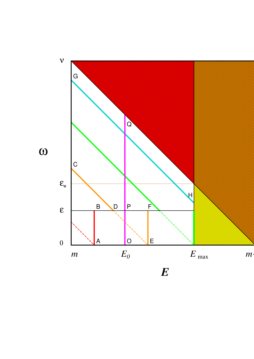
Figure 6: The $E$–$\omega$ plane for $E\in[m,m+\nu]$ and $\omega\in[0,\nu]$. See text for details.

Figure 6 shows the $E$–$\omega$ plane for $E\in[m,m+\nu]$ and $\omega\in[0,\nu]$ ($E$, however, cannot exceed its elastic endpoint $E_{\rm\scriptstyle max}$). For a moment we will assume (as we did in drawing fig. 6) that $\epsilon$ is smaller than $\epsilon_{\star}=\nu^{\prime}_{\rm\scriptstyle min}$, but we will later on free our analysis from this constraint. The vertical segments OP and PQ indicate, respectively, the sets of points contributing to the VS and HB corrections to the electron spectrum (see sect. 3) for a specific value $E=E_{0}$ (in the virtual corrections it’s simply $\omega=0$). The overall QED corrections to the electron spectrum are obtained by adding up the VS and HB terms and clearly do not depend on the value of $\epsilon$. In fig. 6, diagonal lines indicate sets of points with the same value of the combined electron–photon energy. The set of all points in the $E$–$\omega$ plane having the same $E_{\omega}$ value consists of one or two segments, according to the magnitude of $E_{\omega}$ which varies between $m$ and $m+\nu$. If $m\leq E_{\omega}<m+\epsilon$, the photon energy is lower than the threshold $\epsilon$ and the measured combined energy $E_{\omega}$ equals $E$. The QED corrections to the differential cross section $d\sigma/dE_{\omega}$ will coincide, in this case, with the VS corrections to the electron spectrum $d\sigma/dE$ (see e.g. segment AB). If $m+\epsilon\leq E_{\omega}\leq E_{\rm\scriptstyle max}$, the QED prediction for $d\sigma/dE_{\omega}$ will consist of two contributions, namely the HB cross section $[d\sigma/d(E+\omega)]_{\rm HB}$ (see e.g. segment CD) plus the VS corrections to $d\sigma/dE$ (segment EF). Finally, if $E_{\rm\scriptstyle max}<E_{\omega}<m+\nu$, $d\sigma/dE_{\omega}$ will be identical to $[d\sigma/d(E+\omega)]_{\rm HB}$ (see e.g. segment GH). It is important to notice that the complete QED prediction for the differential cross section with respect to $E_{\omega}$ depends on the threshold $\epsilon$, contrary to the complete QED prediction for the electron spectrum computed in sect. 3.

We can summarize our results in a very simple way. The SM prediction for the spectrum of the combined energy of electron and photon in reaction (8) can be cast, up to corrections of $O(\alpha)$, in the form

$$\left[\frac{d\sigma}{dE_{\omega}}\right]_{\rm SM}\!\!\!\! = \!\!\frac{2mG_{\mu}^{2}}{\pi}\Biggl{\{}g_{\scriptscriptstyle L}^{2}(E_{\omega})\!\left[\theta+\frac{\alpha}{\pi}\bar{f}_{\scriptscriptstyle L}(E_{\omega},\epsilon,\nu)\right]+g_{\scriptscriptstyle R}^{2}(E_{\omega})\left(1-z_{\omega}\right)^{2}\!\left[\theta+\frac{\alpha}{\pi}\bar{f}_{\scriptscriptstyle R}(E_{\omega},\epsilon,\nu)\right]$$ (14)

$$-g_{\scriptscriptstyle L}(E_{\omega})g_{\scriptscriptstyle R}(E_{\omega})\left(\frac{mz_{\omega}}{\nu}\right)\!\left[\theta+\frac{\alpha}{\pi}\bar{f}_{{\scriptscriptstyle L}{\scriptscriptstyle R}}(E_{\omega},\epsilon,\nu)\right]\Biggr{\}},$$

where $z_{\omega}=(E_{\omega}-m)/\nu$ and $\theta=\theta(E_{\rm\scriptstyle max}-E_{\omega})$. As we mentioned in sect. 3, the deviations of the functions $g_{\scriptscriptstyle L}(E_{\omega})$ and $g_{\scriptscriptstyle R}(E_{\omega})$ from the lowest–order values $g_{\scriptscriptstyle L}$ and $g_{\scriptscriptstyle R}$ reflect the effect of the electroweak corrections (for virtual corrections it is $\omega=0$ and $E_{\omega}=E$). The functions $\bar{f}_{\scriptscriptstyle X}(E_{\omega},\epsilon,\nu)$ ($X=L,R$ or $LR$), defined in the range $[m,m+\nu]$, describe the QED effects discussed earlier in this section (once again, for simplicity of notation, we will drop their $\nu$ dependence). Following our previous analysis, these functions can be written in the very simple form

$$\bar{f}_{\scriptscriptstyle X}(E_{\omega},\epsilon)=f_{\scriptscriptstyle X}^{\scriptscriptstyle VS}(E_{\omega},\epsilon)+\bar{f}_{\scriptscriptstyle X}^{\scriptscriptstyle HB}(E_{\omega},\epsilon),$$ (15)

where $f_{\scriptscriptstyle X}^{\scriptscriptstyle VS}(E_{\omega},\epsilon)$ are the “exact” VS corrections of sect. 3 (eq. (12)) and the functions $\bar{f}_{\scriptscriptstyle X}^{\scriptscriptstyle HB}(E_{\omega},\epsilon)$ are derived by dividing the $L$, $R$ and $LR$ parts of the above–studied HB cross section $[d\sigma/d(E+\omega)]_{\rm HB}$ by $Cg_{\scriptscriptstyle L}^{2}$, $Cg_{\scriptscriptstyle R}^{2}(1-z_{\omega})^{2}$ and $-Cg_{\scriptscriptstyle L}g_{\scriptscriptstyle R}(mz_{\omega}/\nu)$ respectively, with $C=2mG_{\mu}^{2}\alpha/\pi^{2}$. The $\theta$ functions in eq. (14) reflect the fact that the lowest order prediction for $d\sigma/dE_{\omega}$ has a step at $E_{\omega}=E_{\rm\scriptstyle max}$ and is zero if $E_{\omega}$ lies outside the elastic range $[m,E_{\rm\scriptstyle max}]$. The VS functions $f_{\scriptscriptstyle X}^{\scriptscriptstyle VS}(E_{\omega},\epsilon)$ are proportional to the same $\theta$ function, while the corrections $\bar{f}_{\scriptscriptstyle X}^{\scriptscriptstyle HB}(E_{\omega},\epsilon)$ are set to zero if $E_{\omega}\in\!\!\!\!\!/\;[m+\epsilon,m+\nu]$.

Earlier in this section we assumed $\epsilon<\epsilon_{\star}$ ($\epsilon_{\star}=\nu^{\prime}_{\rm\scriptstyle min}$). Nevertheless, the $\epsilon_{\star}\leq\epsilon\leq\nu$ case can be discussed analogously and our simple prescription (15) is valid in both cases.

In fig. 7 we show, as an example, the function $\bar{f}_{\scriptscriptstyle L}(E_{\omega},\epsilon)$ (thick) and its components $\bar{f}_{\scriptscriptstyle L}^{\scriptscriptstyle HB}(E_{\omega},\epsilon)$ (medium) and $f_{\scriptscriptstyle L}^{\scriptscriptstyle VS}(E_{\omega},\epsilon)$ (thin) for $\nu=0.862\mbox{ MeV}$. The solid (dashed) lines correspond to the choice $\epsilon=0.2\mbox{ MeV}$ ($\epsilon=0.05\mbox{ MeV}$). Once again we would like to emphasize the $\epsilon$ dependence of the complete QED corrections $\bar{f}_{\scriptscriptstyle X}(E_{\omega},\epsilon)$, to be contrasted with the $\epsilon$ independence of the $f_{\scriptscriptstyle X}(E)$ functions of sect. 3.

In figs. 8, 9 and 10 we compare the results of sects. 3 and 4. In fig. 8 we chose $\nu=0.862\mbox{ MeV}$ and plotted the functions $f_{\scriptscriptstyle X}(E)$ (thick) and $\bar{f}_{\scriptscriptstyle X}(E_{\omega},\epsilon)$ for $\epsilon=$ 0.1 MeV (medium) and 0.001 MeV (thin). In figs. 9 and 10 we plotted the same functions with $\nu=10\mbox{ MeV}$ ($\epsilon=$ 1 MeV, 0.1 MeV) and $\nu=1\mbox{ GeV}$ ($\epsilon=$ 100 MeV, 10 MeV), respectively.

We would like to remind the reader that the functions $f_{\scriptscriptstyle X}(E)$ can be obtained from $\bar{f}_{\scriptscriptstyle X}(E_{\omega},\epsilon)$ by simply setting $\epsilon=\nu$. The limiting case $\epsilon=0$ was studied in detail in ref. [12] (in particular, the results of the second article of this reference were obtained, like ours, without employing the ultrarelativistic approximation $E\gg m$).

5 Discussion and Conclusions

When are the results of sects. 2, 3 and 4 applicable? In sects. 2 and 3 we evaluated the $O(\alpha)$ SM prediction for the electron spectrum in the reaction $\nu_{l}+e\rightarrow\nu_{l}+e\;(+\gamma)$ (eq. (9)), where $(+\gamma)$ indicates the possible emission of a photon. In this calculation we assumed that the final–state photon is not detected and, as a consequence, we integrated over all possible values of the photon energy $\omega$. Therefore, eq. (9) is the appropriate theoretical prediction to use in the analysis of $\nu$–$e$ scattering when the detector is completely blind to photons of all energies, but can precisely measure $E$, the energy of the electron. Of course, a detector could provide more information by detecting photons as soon as their energy is above an experimental threshold $\epsilon$. In this case, still assuming a precise determination of $E$, one can employ eq. (9), minus its HB correction, to analyze those events which are counted as nonradiative (elastic), while the HB part can be used, at least in principle, for a separate determination of the inelastic cross section. Indeed, contrary to previous calculations, our predictions are valid for an arbitrary value of the threshold $\epsilon$ (and include the previously unknown $LR$ term).

In sect. 4 we evaluated the spectrum of the total combined energy of the recoil electron and a possible accompanying photon emitted in the scattering process (eq. (14); $E_{\omega}$ was defined in eq. (13)). This type of analysis is useful when the photon energy $\omega$ cannot be separately determined although it fully contributes to the precise total energy measurement if its value is above a specific threshold $\epsilon$. Let’s consider an experimental setup able to measure the photon energy if it’s higher than $\epsilon$, but completely blind to low energy photons $(\omega\!<\!\epsilon)$. Let’s also assume that the electron energy $E$ is precisely measurable independently of its value. This detector can determine both the differential cross section $d\sigma/dE_{\omega}$ (eq. (14)) and the electron spectrum $d\sigma/dE$ (eq. (9)) (as well as its separate HB component). There are experiments, however, which cannot measure $E$, but only $E_{\omega}$, with a specific value of the threshold $\epsilon$. BOREXINO [25] and KamLAND [26], for example, are liquid scintillation detectors in which photons and electrons induce practically the same response. If a photon is emitted in the $\nu$–$e$ scattering process, its energy $\omega$ is counted together with $E$, provided their sum lies within a specific range. The appropriate theoretical prediction for their analysis is given, therefore, by the cross section $d\sigma/dE_{\omega}$ of eq. (14) with a very small value of $\epsilon$ (for the case $\nu=0.862\mbox{ MeV}$ see the thin lines in fig. 8). However, we should point out that although the QED corrections $f_{\scriptscriptstyle X}(E)$ (in eq. (9)) and $\bar{f}_{\scriptscriptstyle X}(E_{\omega},\epsilon)$ with small $\epsilon$ (in eq. (14)) are different, their numerical values are very small when $\nu=0.862\mbox{ MeV}$, the energy of the monochromatic neutrinos produced by electron capture on $\!\!\!\!\phantom{A}{}^{7}$Be in the solar interior. In fact, as shown in fig. 8, both $(\alpha/\pi)f_{\scriptscriptstyle X}(E)$ and $(\alpha/\pi)\bar{f}_{\scriptscriptstyle X}(E_{\omega},\epsilon)$ with small $\epsilon$ are in this case of $O(\raisebox{-3.01385pt}{$\stackrel{{\scriptstyle\textstyle<}}{{\sim}}\,$}1\%)$, and neither of the above collaborations is likely to reach this high level of accuracy in their analyses of the crucial $\!\!\!\!\phantom{A}{}^{7}$Be line.

There are detectors in which it might not be possible to identify the measured energy with either $E$ or $E_{\omega}$. Indeed, the electron and the photon may produce indistinguishable signals and the total observed energy might not be the simple sum of $E$ and $\omega$, but some other function of these two variables. Super–Kamiokande (SK)[21], for example, a water Cherenkov counter measuring the light emitted by electrons recoiling from neutrino scattering, uses the number of hit photomultiplier tubes to determine the electron energy. However, a photon emitted in the scattering process may induce additional hits indistinguishable from those of the electron. Moreover, a photon and an electron of the same energy may produce different numbers of hits and, therefore, it might not be possible to identify the total measured energy with the sum $E+\omega$.

SK measures solar neutrinos with energies varying from 5 to 18 MeV. For $\nu=10\mbox{ MeV}$, fig. 9 shows that the QED corrections to the differential cross sections $d\sigma/dE$ (eq. (9)) and $d\sigma/dE_{\omega}$ (eq. (14)) are of $O(1\%)$. Corrections of this order may be relevant for the analysis of the very precise data obtained by this collaboration. In fact, SK’s Monte Carlo simulations of the expected energy spectrum of recoil electrons from solar neutrino scattering include the QED corrections of ref. [16] (as well as the EW ones). As we investigated in sect. 3, these corrections provide good approximations of the complete $O(\alpha)$ QED corrections $f_{\scriptscriptstyle X}(E)$ to the electron spectrum of eq. (9) (see fig. 4). Our previous discussion, however, seems to suggest that these corrections may not be appropriate for SK’s solar neutrino analysis. On the other hand, the SM prediction for the spectrum of the combined energy of electron and photon of sect. 4 (eq. (14)) may be suitable, but only if we can assume a similar efficiency in the detection of photons and electrons, and if also relatively low energy electrons contribute to the total energy measurement. If these conditions are not met, and the precision of the data requires it, one should probably perform a dedicated analysis of the double differential cross section $d^{2}\sigma/(dE\,d\omega)$ with a response function specifically designed for this detector. A triple differential cross section $d^{3}\sigma/(dE\,d\omega\,d\phi)$, where $\phi$ is the angle between the directions of the electron and the photon, may also be useful (see the third article of ref. [4], and ref. [13]).

We will conclude by noticing that the QED corrections, contrary to the EW ones, depend strongly on the initial neutrino energy and become sizeable at high energies. Their appropriate expression will have to be taken into account in the analysis of future precise high energy $\nu$–$e$ scattering experiments.

Acknowledgments

I would like to thank Prof. J. N. Bahcall and Prof. A. Sirlin for suggesting this problem and for enlightening discussions. I am particularly indebted to Prof. P. Minkowski and Prof. A. Sirlin for reading the manuscript and for very useful comments. I would also wish to express my gratitude to J. Arafune, D. Bardin, C. Greub, A. Held, K. Holland, T. Kinoshita, W. Marciano, M. Nakahata, J. Papavassiliou, M. Samaras, M. Schaden, S. Schoenert, Y. Takeuchi and Y. Totsuka for instructive conversations and exchanges of ideas. This work was supported by Schweizerischer Nationalfonds.

Figure 1: Comparison of the $f_{\scriptscriptstyle X}^{\scriptscriptstyle HB}(E,\epsilon)$ functions (solid lines) with their small $\epsilon$ analytic approximations (dotted lines) for an initial neutrino energy $\nu=$ 0.862 MeV. Thick, normal and thin lines indicate, respectively, $\epsilon=$ 0.001, 0.01 and 0.1 MeV.

Figure 2: Comparison of the $f_{\scriptscriptstyle X}^{\scriptscriptstyle HB}(E,\epsilon)$ functions (solid lines) with their small $\epsilon$ analytic approximations (dotted lines) for an initial neutrino energy $\nu=$ 10 MeV. Thick, normal and thin lines indicate, respectively, $\epsilon=$ 0.5, 1 and 2 MeV.

Figure 3: The functions $f_{\scriptscriptstyle X}(E)$ (thick solid), $f_{\scriptscriptstyle X}^{\scriptscriptstyle HB}(E,\epsilon)$ (medium solid) and $f_{\scriptscriptstyle X}^{\scriptscriptstyle VS}(E,\epsilon)$ (thin solid) for $\nu=$ 0.862 MeV and $\epsilon=$ 0.02 MeV. The dotted lines represent the $f_{\scriptscriptstyle X}(E)$ approximations of ref. [16]. In the $LR$ figure, the dot-dashed line is the product of the $f_{{\scriptscriptstyle L}{\scriptscriptstyle R}}(E)$ approximation of ref. [16] and $(mz/\nu)$, while the dashed line indicates the product $(mz/\nu)f_{{\scriptscriptstyle L}{\scriptscriptstyle R}}(E)$.

Figure 4: Same as Fig. 3, but for $\nu=$ 10 MeV and $\epsilon=$ 1 MeV. The dashed and dot-dashed lines are very close to zero and are not indicated.

Figure 5: Same as Fig. 3, but for $\nu=$ 1 GeV and $\epsilon=$ 50 MeV. The dashed and dot-dashed lines are very close to zero and are not indicated.

Figure 7: The function $\bar{f}_{\scriptscriptstyle L}(E_{\omega},\epsilon)$ (thick) and its components $\bar{f}_{\scriptscriptstyle L}^{\scriptscriptstyle HB}(E_{\omega},\epsilon)$ (medium) and $f_{\scriptscriptstyle L}^{\scriptscriptstyle VS}(E_{\omega},\epsilon)$ (thin) for $\nu=$ 0.862 MeV. Solid and dashed lines indicate, respectively, $\epsilon=$ 0.2 and 0.05 MeV.

Figure 8: The functions $f_{\scriptscriptstyle X}(E)$ (thick) and $\bar{f}_{\scriptscriptstyle X}(E_{\omega},\epsilon)$ for $\epsilon=$ 0.1 MeV (medium) and 0.001 MeV (thin). $\nu=$ 0.862 MeV.

Figure 9: The functions $f_{\scriptscriptstyle X}(E)$ (thick) and $\bar{f}_{\scriptscriptstyle X}(E_{\omega},\epsilon)$ for $\epsilon=$ 1 MeV (medium) and 0.1 MeV (thin). $\nu=$ 10 MeV.

Figure 10: The functions $f_{\scriptscriptstyle X}(E)$ (thick) and $\bar{f}_{\scriptscriptstyle X}(E_{\omega},\epsilon)$ for $\epsilon=$ 100 MeV (medium) and 10 MeV (thin). $\nu=$ 1 GeV.

References

- [1] T. D. Lee and A. Sirlin, Rev. Mod. Phys. 36 (1964) 666.
- [2] M. Ram, Phys. Rev. 155 (1967) 1539.
- [3] G. ’t Hooft, Phys. Lett. B37 (1971) 195.
- [4] E. D. Zhizhin, R. V. Konoplich, Yu. P. Nikitin, and B. U. Rodionov, ZhETF Pis. Red. 19 (1974), No.1, pp. 57–60 [JETP Lett. 19 (1974) 36]; E. D. Zhizhin, R. V. Konoplich, and Y. P. Nikitin, Izv. VUZ, Fiz. (1975), No.12, pp. 82–89 [Sov. Phys. J. 18 (1975), No.12, 1709]; Elementary Particles and Cosmic Rays, Atomizdat, Moscow (1976), pp. 57–71 (in Russian).
- [5] P. Salomonson and Y. Ueda, Phys. Rev. D11 (1975) 2606.
- [6] M. Green and M. Veltman, Nucl. Phys. B169 (1980) 137; Erratum–ibid. B175 (1980) 547.
- [7] W. J. Marciano and A. Sirlin, Phys. Rev. D22 (1980) 2695.
- [8] K. Aoki, Z. Hioki, R. Kawabe, M. Konuma and T. Muta, Prog. Theor. Phys. 65 (1981) 1001.
- [9] K. Aoki and Z. Hioki, Prog. Theor. Phys. 66 (1981) 2234; Z. Hioki, Prog. Theor. Phys. 67 (1982) 1165.
- [10] S. Sarantakos, A. Sirlin and W.J. Marciano, Nucl. Phys. B217 (1983) 84.
- [11] D. Y. Bardin and V. A. Dokuchaeva, Yad. Fiz. 39 (1984) 888 [Sov. J. Nucl. Phys. 39 (1984) 563].
- [12] D. Y. Bardin and V. A. Dokuchaeva, Nucl. Phys. B246 (1984) 221; Yad. Fiz. 43 (1986) 1513 [Sov. J. Nucl. Phys. 43 (1986) 975].
- [13] J. Bernabeu, S. M. Bilenky, F. J. Botella and J. Segura, Nucl. Phys. B426 (1994) 434.
- [14] J. Bernabeu, L. G. Cabral-Rosetti, J. Papavassiliou and J. Vidal, Phys. Rev. D62 (2000) 113012.
- [15] J. N. Bahcall, Rev. Mod. Phys. 59 (1987) 505.
- [16] J. N. Bahcall, M. Kamionkowski and A. Sirlin, Phys. Rev. D51 (1995) 6146.
- [17] A. Sirlin, Rev. Mod. Phys. 50 (1978) 573; Phys. Rev. D22 (1980) 971.
- [18] A. Ferroglia, G. Ossola and A. Sirlin, Nucl. Phys. B560 (1999) 23.
- [19] R. Mertig, M. Bohm and A. Denner, Comput. Phys. Commun. 64 (1991) 345.
- [20] G. P. Lepage, J. Comput. Phys. 27 (1978) 192; CLNS-80/447 (1980).
- [21] Super-Kamiokande Collaboration, Y. Fukuda et al., Phys. Rev. Lett. 81 (1998) 1158; Erratum–ibid. 81 (1998) 4279; Phys. Rev. Lett. 82 (1999) 2430; Y. Suzuki and Y. Totsuka (Eds.), Neutrino 98, Proceedings of the XVIII International Conference on Neutrino Physics and Astrophysics, Takayama, Japan, June 4-9, 1998, Nucl. Phys. Proc. Suppl. 77 (1999); Y. Suzuki, Nucl. Phys. Proc. Suppl. 91 (2001) 29.
- [22] R. E. Behrends, R. J. Finkelstein and A. Sirlin, Phys. Rev. 101 (1956) 866.
- [23] T. Kinoshita and A. Sirlin, Phys. Rev. 113 (1959) 1652.
- [24] T. Kinoshita, J. Math. Phys. 3 (1962) 650; T. D. Lee and M. Nauenberg, Phys. Rev. 133 (1964) B1549.
- [25] G. Ranucci et al. [BOREXINO Collaboration], Nucl. Phys. Proc. Suppl. 91 (2001) 58.
- [26] A. Piepke [KamLAND Collaboration], Nucl. Phys. Proc. Suppl. 91 (2001) 99.