FERMILAB-Conf-00/298-T hep-ph/0011181

$|V_{ub}|$ From Semileptonic Decay and $b\to s\gamma$

Adam K. Leibovich

Department of Physics,Carnegie Mellon University, Pittsburgh, PA 15213
Theory Group, Fermilab, P.O. Box 500, Batavia, IL 60510

Current errors on $|V_{ub}|$ are dominated by model dependence. For inclusive decays, the model dependence comes from the Fermi motion of the $b$ quark. By combining the endpoint photon and lepton spectra from the inclusive decays $B\rightarrow X_{s}\,\gamma$ and $B\rightarrow X_{u}\,\ell\,\overline{\nu}$, it is possible to remove this model dependence. We show how to combine these rates including the resummation of the endpoint logs at next to leading order. The theoretical errors on $|V_{ub}|$ on the order of 10% are possible. We also give a brief discussion on comparing different extractions.

Presented at the

5th International Symposium on Radiative Corrections
(RADCOR–2000)
Carmel CA, USA, 11–15 September, 2000

1 Introduction

The Cabibbo-Kobayashi-Maskawa matrix element $V_{ub}$ is very important for understanding CP violation in the Standard Model. An accurate measurement of $|V_{ub}|$ puts strong constraints on the Unitarity Triangle. Unfortunately, $V_{ub}$ is vary hard to measure. Current measurements have errors that are dominated by model dependence. Some of the best extractions so far have come from exclusive decays, such as $B\to\pi\ell\overline{\nu}$ or $B\to\rho\ell\overline{\nu}$. The problem with exclusive decays is the strong hadronic dynamics can not be calculated, and we have to resort to models, light-cone sum rules, or lattice QCD calculations to obtain the form factors [1]. At the present time, all these methods give around 20% errors. A recent measurement from CLEO [2] using $B\to\rho\ell\overline{\nu}$ gives $|V_{ub}|=[3.25\pm 0.14{\rm(stat.)}^{+0.21}_{-0.29}{\rm(syst.)}\pm 0.55{\rm(model)}]\times 10^{-3}$. In the future, the lattice will give accurate predictions for the form factors, but until then, a measurement of 20% is probably the best we can hope for from exclusive decays.

In some ways, inclusive decays should provide a straightforward means to measure $|V_{ub}|$. All we need to do is measure the total rate $b\to u\ell\overline{\nu}$, which is proportional to $|V_{ub}|^{2}$ and is known to order $\alpha_{s}^{2}$ [3]. If we could measure the total rate, we would not have to worry about quark-hadron duality violations, thus a very accurate measurement would be possible.

Unfortunately, there is a very large background from $b\to c$ decays, which is about 100 times more abundant than $b\to u$ decays. To remove this large background, kinematic cuts must be made. Three basic cuts are discussed in the literature, each having its own advantages: a cut on the electron energy spectrum, a cut on the hadronic invariant mass spectrum, and a cut on the leptonic invariant mass spectrum. For now we will concentrate on the electron energy spectrum, and return to the other cuts later.

Since the $u$ quark is much lighter than the $c$ quark, the electron energy spectrum for $b\to u$ decays extends past the endpoint for $b\to c$ decays, see Fig. 1. Thus it is possible to remove the charm quark background by cutting above the $b\to c$ endpoint.

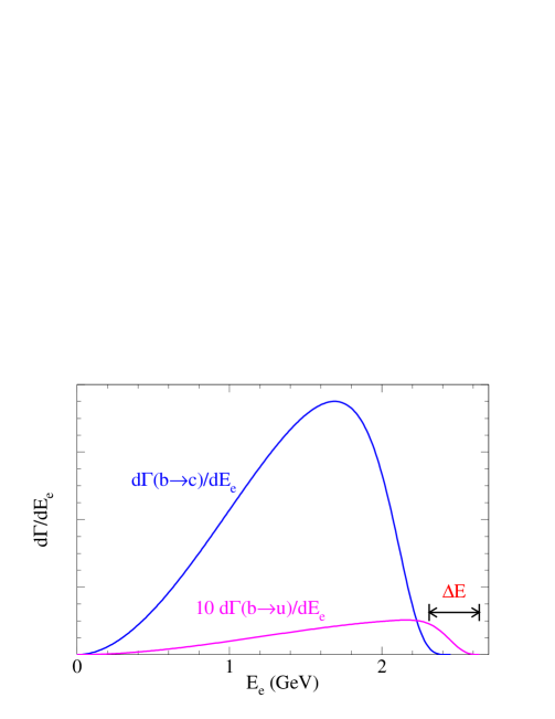
Figure 1: Electron spectrum for semi-leptonic $b$ decay rates to $c$ and $u$ quarks. The rate for $b\to ue\overline{\nu}$ has been multiplied by a factor of 10. The region in $\Delta E$ can only have $b\to u$ decays, and thus is useful for extracting $|V_{ub}|$.

All that is necessary is a theoretical prediction for the integrated rate above the cut. Unfortunately, putting a cut near the endpoint introduces a new small mass scale, $\Delta E\sim 300{\rm\ MeV}$, which introduces large perturbative $[\log(m_{b}/\Delta E)]$ and non-perturbative ($\Lambda/\Delta E)$ corrections. Therefore both the perturbative and non-perturbative series must be resummed for the rate to be trustworthy.

The calculation of the rate begins with the effective Hamiltonian [4]

$$H_{eff} = \frac{-4G_{F}}{\sqrt{2}}V_{ub}(\overline{u}\gamma_{\mu}P_{L}b)(\overline{\ell}\gamma^{\mu}P_{L}\nu_{\ell})$$ (1)

$$= \frac{-4G_{F}}{\sqrt{2}}V_{ub}J_{\mu}J^{\mu}_{\ell},$$

obtained by integrating out the $t$ quark and $W$ bosons. The differential decay distribution can then be written as the product of leptonic and hadronic tensors

$$d\Gamma\propto|V_{ub}|^{2}L^{\alpha\beta}W_{\alpha\beta}.$$ (2)

Using the Optical Theorem, the hadronic tensor $W_{\alpha\beta}$ can be related to the imaginary part of the time ordered product of currents

$$W_{\alpha\beta} = -\frac{1}{\pi}{\rm Im}\,T_{\alpha\beta},$$ (3)

$$T_{\alpha\beta} = -\frac{i}{2M_{B}}\int d^{4}xe^{-iq\cdot x}\langle B|T(J_{\alpha}^{\dagger}(x)J_{\beta}(0))|B\rangle.$$ (4)

The time ordered product can be calculated by expanding in an Operator Product Expansion (OPE). The Wilson coefficients can be calculated (over most of phase space) in perturbation theory [5, 6], while higher dimensional operators in the OPE are suppressed (over most of phase space) by powers of $1/m_{b}$. Thus, the leading term in the OPE gives free $b$ quark decay. The first corrections enter at order $1/m_{b}^{2}$, and are proportional to the Heavy Quark Effective Theory parameters

$$\lambda_{1} = \frac{\langle B|\overline{h}_{v}(iD)^{2}h_{v}|B\rangle}{2M_{B}},$$ (5)

$$\lambda_{2} = \frac{\langle B|\overline{h}_{v}g\sigma_{\mu\nu}G^{\mu\nu}|B\rangle}{12M_{B}}.$$ (6)

The problems begin as the energy of the lepton approaches the endpoint. Defining $x=2E_{\ell}/m_{b}$ to be the rescaled lepton energy, the higher dimensional operators in the OPE are actually suppressed by

$$\frac{\Lambda}{m_{b}(1-x)}\to 1\qquad{\rm as\ }x\to 1.$$ (7)

Higher dimensional operators in the expansion are no longer suppressed. In other words, the expansion is becoming singular as we approach the endpoint.

The breakdown in the OPE can be seen in the expression for the rate at order $1/m_{b}^{2}$ [7],

$$\left.\frac{d\Gamma}{dx}\right|_{O(1/m_{b}^{2})}\propto\frac{5\lambda_{1}+33\lambda_{2}}{3m_{b}^{2}}\theta(1-x)-\frac{\lambda_{1}+33\lambda_{2}}{6m_{b}^{2}}\delta(1-x)-\,\frac{\lambda_{1}}{6m_{b}^{2}}\delta^{\prime}(1-x),$$ (8)

by the appearance of singular functions at the endpoint.

To handle the breakdown of the non-perturbative series, the leading singular terms must be resummed. These corrections resum into a non-perturbative structure function, $f(k_{+})$ [8]. The differential rate is now a convolution of $f(k_{+})$ with the partonic rate [8, 9]

$$\frac{d\Gamma}{dE_{\ell}}=\int dk_{+}\,f(k_{+})\frac{d\Gamma_{p}}{dE_{\ell}}(m_{b}^{*}),$$ (9)

where $m_{b}^{*}=m_{b}+k_{+}$. The structure function is universal, meaning that the same function occurs for $b\to u\ell\overline{\nu}$ and $b\to s\gamma$ decays. Being a non-perturbative function, $f(k_{+})$ is not known; we do know the first few moments of $f(k_{+})$, however. Thus, to handle the endpoint region, some model for $f(k_{+})$ must be introduced. We could in principle extract the structure function from $b\to s\gamma$ decays and then apply it to $b\to u\ell\overline{\nu}$, but this is difficult because of the way $f(k_{+})$ enters the rate (9). Instead, we will skip the step of extracting the structure function and directly use the $b\to s\gamma$ rate in the $b\to u\ell\overline{\nu}$ rate. But first we need to discuss the perturbative corrections.

Near the endpoint, the perturbative correction to the rate looks like [10]

$$\frac{d\Gamma}{dx}\propto 1-\frac{2\alpha_{s}}{3\pi}\left[\log^{2}(1-x)+\frac{31}{6}\log(1-x)+\pi^{2}+\frac{5}{4}\right].$$ (10)

As $x\to 1$, the logs become large and the perturbative series breaks down. To trust the prediction, the logs need to be resummed. There are similarly large logs in the rate for $b\to s\gamma$, so the logs must be resummed there, too [11].

It is possible to resum the series using Infrared Factorization, which is also used for DIS, Drell-Yan, etc. The idea is that in the endpoint region, the light quark is shot out with large energy, but with small invariant mass. This quark produces a jet of particles through collinear radiation. While the constituents of the jet can talk to each other (and the original $b$ quark) through soft gluons, hard gluon exchange is disallowed. The soft radiation cannot tell if the jet was initiated by a $u$ quark or an $s$ quark, thus it will be the same for $b\to u$ and $b\to s$ decays.

Mathematically, there is a separation of momentum regions into [12]

$${\rm Hard}\ (H): k_{+}\sim k_{-}\sim k_{t}=O(m_{b}),$$ (11)

$${\rm Jet}\ (J): k_{+}=O[m_{b}(1-x)],\ k_{-}=O(m_{b}),k_{t}=O(m_{b}\sqrt{1-x}),$$ (12)

$${\rm Soft}\ (S): k_{+}\sim k_{-}\sim k_{t}=O[m_{b}(1-x)].$$ (13)

By introducing a factorization scale $\mu$ to keep these regions separated, we can write the rate in factorized form as

$$\frac{d\Gamma}{dx}\sim\int dzS(z,\mu)J(z,\mu)H(\mu).$$ (14)

The soft function $S(z,\mu)$ is the same for $b\to u$ and $b\to s$, while $J(z,\mu)$ and $H(\mu)$ depend on the process.

The rate completely factorizes after taking moments,

$$M_{N}^{\gamma} = \int_{o}^{M_{B}/m_{b}}dx\,x^{n-1}\,\frac{1}{\Gamma_{o}^{\gamma}}\frac{d\Gamma^{\gamma}}{dx}=S_{N}J_{N}^{\gamma}H_{N}^{\gamma},$$ (15)

$$M_{N}^{sl} = -\int_{o}^{M_{B}/m_{b}}dx\,x^{n-1}\,\frac{1}{\Gamma_{o}^{\gamma}}\frac{d}{dx}\frac{d\Gamma^{\gamma}}{dx}$$ (16)

$$= \int dx_{\nu}S_{N}J_{N}^{sl}(x_{\nu})H_{N}^{sl}(x_{\nu}),$$

where $M_{N}^{\gamma}$ and $M_{N}^{sl}$ are the moments of the $b\to s\gamma$ and $b\to u\ell\overline{\nu}$ rates, respectively.

The soft function contains perturbative and non-perturbative pieces

$$S_{N}=f_{N}\sigma_{N},$$ (17)

where $f_{N}$ are the moments of the structure function introduced earlier. Thus we can write the moments (15) and (16) as

$$M_{N}^{\gamma} = f_{N}\sigma_{N}J_{N}^{\gamma}H_{N}^{\gamma},$$ (18)

$$M_{N}^{sl} = \int dx_{\nu}f_{N}\sigma_{N}J_{N}^{sl}(x_{\nu})H_{N}^{sl}(x_{\nu}).$$ (19)

All the large logarithms are contained in the combination $\sigma_{N}J_{N}$. The only fact we need about the perturbative resummation is that after resumming, including next-to-leading logarithms, there is the relation [13]

$$\sigma_{N}J_{N}^{sl}=\sigma_{N}J_{N}^{\gamma}\exp[g_{sl}(\alpha_{s}\log N)],$$ (20)

where $\exp[g_{sl}(\alpha_{s}\log N)]$ is a known function.

We can now combine the above results. Substituting first (20) into (19), and then (18) into the result, we get

$$M_{N}^{sl} = \int dx_{\nu}f_{N}\sigma_{N}J_{N}^{sl}(x_{\nu})H_{N}^{sl}(x_{\nu})$$ (21)

$$= \int dx_{\nu}f_{N}\sigma_{N}J_{N}^{\gamma}\exp[g_{sl}(\alpha_{s}\log N)]H_{N}^{sl}(x_{\nu})$$

$$= \int dx_{\nu}\frac{M_{N}^{\gamma}}{H^{\gamma}}\exp[g_{sl}(\alpha_{s}\log N)]H_{N}^{sl}(x_{\nu}).$$

Note that the dependence on the unknown structure function $f_{N}$ has been eliminated.

We can go back to $x$-space by taking an inverse Mellin transform. The left-hand side of (21) is just the semi-leptonic rate. The right-hand side is a convolution of the $b\to s\gamma$ rate with a known function. Rearranging, we can write this as [14]

$$\frac{|V_{ub}|^{2}}{|V_{ts}^{*}V_{tb}|^{2}}=\frac{\int\Gamma(b\to u\ell\nu)}{\int\int d\Gamma^{\gamma}/dx^{\gamma}*K(x^{\gamma},\alpha_{s})}.$$ (22)

So in words, what we have done is written $|V_{ub}|^{2}$ as the ratio of the $b\to ue\overline{\nu}$ rate over a convolution of the $b\to s\gamma$ rate with a known function.

What are the uncertainties? First, there are higher order corrections that we neglected, which enter at the order of $\Lambda/m_{b}$, $\alpha_{s}(1-x)$ and $(1-x)^{3}$. For the value of the electron energy cut, $x_{\rm cut}\approx 0.87$, these corrections should all be less that 10%. Of course, we are estimating the size of the higher order corrections, since they have not been calculated. They may be larger or smaller by a factor of 2 or 3. Without calculating the corrections directly, it is not possible to know. We will come back to this qualification shortly.

Second, there are the violations of quark-hadron duality. These violations are hard to quantify, but they should be small if we are not dominated by a just a few resonances; the more final states, the smaller the duality violations. In the region that we are interested in, it does not appear that we are dominated by resonances, so neglecting them should be okay. It would be better if we could have a larger number of the decay products.

This is possible if we cut on different kinematic variables. The other variables discussed in the literature are the hadronic invariant mass [15], and the lepton invariant mass [16]. The hadronic invariant mass spectrum also has dependence on the structure function [15, 17], which introduces model dependence. However, by using a method analogous to the one described above for the electron spectrum, the dependence on the structure function can be eliminated [18, 19]. The errors from higher order corrections are similar to the electron spectrum and should be around 10%. The main advantage of the hadronic invariant mass is that after a cut to remove the charm background, between 40% and 80% of the possible final states will be included. This is much larger than for the electron spectrum, which includes about 10% of the possible final states. Thus the quark-hadron duality violations should be negligible.

The leptonic invariant mass cut has different advantages [16, 20]. Here the structure function is not important, so we do not need to do anything to remove this model dependence. Higher order non-perturbative corrections are on the order of $(\Lambda/m_{c})^{3}$, which leads to an error again of around 10%. This disadvantage for this cut is the fraction of final states included after the cut is around 20%, so the quark-hadron duality errors may be an issue. There is also some question about how good a resolution can be obtained on the lepton invariant mass, which is the only immediate problem for this method.

All three of the above methods should have a theoretical uncertainty (modulo quark-hadron duality violations) of around 10%. Again, these are estimates of higher order corrections. The actual errors may be bigger or smaller. Also, the duality violations could enter in different ways for each measurement. To really trust any extraction of $|V_{ub}|$, we should measure it as many ways as possible, and only after (or if) there is a convergence of the results should we trust the extracted value.

Acknowledgments

I would like to my collaborators I. Low and I. Z. Rothstein, and the organizers of Radcor 2000 for a very enjoyable conference.

References

- [1] For a recent review on methods for extracting along with reasonable assessments of theory errors, see Z. Ligeti, hep-ph/9908432.
- [2] B. H. Behrens et al. [CLEO Collaboration], Phys. Rev. D61, 052001 (2000).
- [3] T. van Ritbergen, Phys. Lett. B454, 353 (1999).
- [4] For a review on calculating the effective weak Hamiltonian, see A. J. Buras, hep-ph/9901409.
- [5] J. Chay, H. Georgi, and B. Grinstein, Phys. Lett. B247 399 (1990); M. Voloshin and M. Shifman, Sov. J. Nucl. Phys. 41 120 (1985).
- [6] I.I. Bigi, M.A. Shifman, N.G. Uraltsev, and A.I. Vainshtein, Int. J. Mod. Phys. A9 2467 (1994).
- [7] A.V. Manohar and M.B. Wise, Phys. Rev. D49 1310 (1994); I.I. Bigi, M. Shifman, N.G. Uraltsev and A.I. Vainshtein, Phys. Rev. Lett. 71 496 (1993); B. Blok, L. Koyrakh, M. Shifman and A.I. Vainshtein, Phys. Rev. D49 (1994), 3356; ERRATUM-ibid. D50 3572 (1994); T. Mannel, Nucl. Phys. B413 396 (1994).
- [8] M. Neubert, Phys. Rev. D49 3392 (1994); T. Mannel and M. Neubert, Phys. Rev. D50 2037 (1994).
- [9] R.D. Dikeman, M. Shifman, and N.G. Uraltsev, Int. J. Mod. Phys. A11 571 (1996).
- [10] M. Jeżabek and J.H. Kühn, Nucl. Phys. B320 961 (1989).
- [11] A. K. Leibovich and I. Z. Rothstein, Phys. Rev. D61, 074006 (2000).
- [12] G. Sterman and G.P. Korchemsky, Phys. Lett. B340 96 (1994).
- [13] R. Akhoury and I.Z. Rothstein, Phys. Rev. D54 2349 (1996).
- [14] A. K. Leibovich, I. Low and I. Z. Rothstein, Phys. Rev. D61, 053006 (2000).
- [15] A. Falk, Z. Ligeti and M.B. Wise, Phys. Lett. 406 225 (1997).
- [16] C. W. Bauer, Z. Ligeti and M. Luke, Phys. Lett. B479, 395 (2000).
- [17] T. Mannel and S. Recksiegel, Phys. Rev. D60 114040 (1999); F. De Fazio and M. Neubert, JHEP 9906, 017 (1999).
- [18] A. K. Leibovich, I. Low and I. Z. Rothstein, Phys. Rev. D62, 014010 (2000).
- [19] A. K. Leibovich, I. Low and I. Z. Rothstein, Phys. Lett. B486, 86 (2000).
- [20] M. Luke, these proceedings.