Charmless decays $B\to PP,PV$, and effects of new strong and electroweak penguins in Topcolor-assisted Technicolor model

Abstract

Based on the low energy effective Hamiltonian with generalized factorization, we calculate the new physics contributions to the branching ratios and CP-violating asymmetries of the two-body charmless hadronic decays $B\to PP,PV$ from the new strong and electroweak penguin diagrams in the Topcolor-assisted Technicolor (TC2) model. The top-pion penguins dominate the new physics corrections, and both new gluonic and electroweak penguins contribute effectively to most decay modes. For tree-dominated decay modes $B\to\pi\pi,\rho\pi,etc,$ the new physics corrections are less than $10\%$. For decays $B\to K^{(*)}\pi$, $K^{(*)}\eta$, $\pi^{0}\eta^{(^{\prime})}$, $\eta^{(^{\prime})}\eta^{(^{\prime})}$, $K\overline{K}^{0}$, $\overline{K}^{*0}K$, $etc$, the new physics enhancements can be rather large ( from $-70\%$ to $\sim 200\%$ ) and are insensitive to the variations of $N_{c}^{eff}$, $k^{2}$, $\eta$ and $m_{\tilde{\pi}}$ within the reasonable ranges. For decays $B^{0}\to\phi\pi$, $\phi\eta^{(^{\prime})}$, $K^{*}\overline{K}^{0}$ and $\rho^{+}K^{0}$, $\delta{\cal B}$ is strongly $N_{c}^{eff}-$dependent: varying from $-90\%$ to $\sim 1680\%$ in the range of $N_{c}^{eff}=2-\infty$. The new physics corrections to the CP-violating asymmetries ${\cal A}_{CP}$ vary greatly for different B decay channels. For five measured CP asymmetries of $B\to K\pi,K\eta^{\prime},\omega\pi$ decays, $\delta{\cal A}_{CP}$ is only about $20\%$ and will be masked by large theoretical uncertainties. The new physics enhancements to interesting $B\to K\eta^{\prime}$ decays are significant in size ($\sim 50\%$), insensitive to the variations of input parameters and hence lead to a plausible interpretation for the unexpectedly large $B\to K\eta^{\prime}$ decay rates. The TC2 model predictions for branching ratios and CP-violating asymmteries of all fifty seven $B\to PP,PV$ decay modes are consistent with the available data within one or two standard deviations.

PACS numbers: 13.25.Hw, 12.15.Ji, 12.38.Bx, 12.60.Nz

1 Introduction

The main goals of B experiments undertaken by CLEO, BarBar, Belle and other collaborations are to explore the physics of CP violation, to test the standard model (SM) at an unexpected level of precision, and to make an exhaustive search for possible effects of physics beyond the SM [1, 2]. Precision measurements of B meson system can provide an insight into very high energy scales via the indirect loop effects of new physics(NP). The B system therefore offers a complementary probe to the search for new physics at the Tevatron, LHC and NLC, and in some cases may yield constraint which surpass those from direct searches or rule out some kinds of NP models[1].

In B experiments, new physics beyond the standard model may manifest itself, for example, in the following ways[1, 3]:

• Decays which are expected to be rare in the standard model are found to have large branching ratios;

• CP-violating asymmetries which are expected to vanish or be very small in the SM are found to be significantly large or with a very different pattern with what predicted in the SM;

• Mixing in B decays is found to differ significantly from SM predictions;

These potential deviations may originate from the virtual effects of new physics through box and/or penguin diagrams in various new physics models [4, 5, 6, 7, 8, 9].

Due to the anticipated importance of two-body charmless hadronic decays $B\to h_{1}h_{2}$ ( where $h_{1}$ and $h_{2}$ are the light pseudo-scalar (P) and/or vector(V) mesons ) in understanding the phenomenon of CP violation, great effort have been made by many authors [10, 11, 12, 13, 14]. It is well known that the low energy effective Hamiltonian is the basic tool to calculate the branching ratios and $A_{CP}$ of B meson decays. The short-distance QCD corrected Lagrangian at NLO level is available now, but we do not know how to calculate hadronic matrix element from first principles. One conventionally resort to the factorization approximation [15]. However, we also know that non-factorizable contribution really exists and can not be neglected numerically for most hadronic B decay channels. To remedy factorization hypothesis, some authors [16, 12, 13] introduced a phenomenological parameter $N_{eff}$ (i.e. the effective number of color) to model the non-factorizable contribution to hadronic matrix element, which is commonly called generalized factorization.

On the other hand, as pointed by Buras and Silverstrini [17], such generalization suffers from the problems of gauge and infrared dependence since the constant matrix $\hat{r}_{V}$ appeared in the expressions of $C_{i}^{eff}$ depends on both the gauge chosen and the external momenta. Very recently, Cheng et al. [18] studied and resolved above controversies on the gauge dependence and infrared singularity of $C_{i}^{eff}$ by using the perturbative QCD factorization theorem. Based on this progress, Chen et al. [14] calculated the charmless hadronic two-body decays of $B_{u}$ and $B_{d}$ mesons within the framework of generalized factorization, in which the effective Wilson coefficients $C_{i}^{eff}$ are gauge invariant, infrared safe, and renormalization-scale and -scheme independent.

On the experimental side, the observation of thirteen $B\to PP,PV$ decays by CLEO, BaBar and Belle collaborations [19, 20, 21, 22, 23, 24, 25] signaled the beginning of the golden age of B physics. For $B\to K\pi,\pi\pi$ decays, the data are well accounted for in the effective Hamiltonian[27, 28] with the generalized factorization approach[15, 12, 14]. For $B\to K\eta^{\prime}$ decays, however, the unexpectedly large decay rate ${\cal B}(B\to K\eta^{\prime})=(80^{+10}_{-9}\pm 7)\times 10^{-6}$ [20] still has no completely satisfactory explanation and has aroused considerable controversy[29].

In this paper, we will present our systematic calculation of branching ratios and CP-violating asymmetries for two-body charmless hadronic decays $B\to PP$, $PV$ (with charged $B_{u}$, neutral $B_{d}$ mesons ) in the framework of Topcolor-assisted technicolor (TC2) model [30] by employing the effective Hamiltonian with the generalized factorization. Since the scale of new strong interactions is expected around $1$ TeV, the tree-level new physics contributions are strongly suppressed and will be neglected. We therefore will focus on the loop effects of new physics on two-body charmless hadronic B meson decays. We will evaluate analytically all new strong and electroweak penguin diagrams induced by exchanges of charged top-pions $\tilde{\pi}^{\pm}$ and technipions $\pi_{1}^{\pm}$ and $\pi_{8}^{\pm}$ in the quark level processes $b\to sV^{*}$ with $V=\gamma,gluon,\;Z$, and then combine the new physics contributions with their SM counterparts, find the effective Wilson coefficients and finally calculate the new physics contributions to the branching ratios and CP-violating asymmetries for all fifty seven decay modes under consideration. We will concentrate on the new physics effects on charmless $B\to PP,PV$ decays and compare the theoretical predictions in TC2 model with the SM predictions as well as the experimental measurements. For the phenomenologically interesting $B\to K\eta^{\prime}$ decays, we found that the new physics enhancements are significant in size, $\sim 50\%$, insensitive to the variations of input parameters and hence lead to a plausible interpretation for the large $B\to K\eta^{\prime}$ decay rates.

This paper is organized as follows. In Sec.2, we describe the basic structures of the TC2 model and examine the allowed parameter space of the TC2 model from currently available data. In Sec.3, we give a brief review about the effective Hamiltonian, and then evaluate analytically the new penguin diagrams and find the effective Wilson coefficients $C_{i}^{eff}$ and effective numbers $a_{i}$ with the inclusion of new physics contributions. In Sec.4 and 5, we calculate and show the numerical results of branching ratios and CP-violating asymmetries for all fifty seven $B\to PP,PV$ decay modes, respectively. We concentrate on modes with well-measured branching ratio and sizable yields. The conclusions and discussions are included in the final section.

2 TC2 model and experimental constraint

Apart from some differences in group structure and/or particle contents, all TC2 models [30, 31] have the following common features: (a) strong Topcolor interactions, broken near 1 TeV, induce a large top condensate and all but a few GeV of the top quark mass, but contribute little to electroweak symmetry breaking; (b) Technicolor [32] interactions are responsible for electroweak symmetry breaking, and Extended Technicolor (ETC) [33] interactions generate the hard masses of all quarks and leptons, except that of the top quarks; (c) there exist top-pions $\tilde{\pi}^{\pm}$ and $\tilde{\pi}^{0}$ with a decay constant $F_{\tilde{\pi}}\approx 50$ GeV. In this paper we will chose the well-motivated and most frequently studied TC2 model proposed by Hill [30] as the typical TC2 model to calculate the contributions to the charmless hadronic B decays in question from the relatively light unit-charged pseudo-scalars. It is straightforward to extend the studies in this paper to other TC2 models.

In the TC2 model[30], after integrating out the heavy coloron and $Z^{\prime}$, the effective four-fermion interactions have the form [34]

$${\cal L}_{eff}=\frac{4\pi}{M_{V}^{2}}\left\{\left(\kappa+\frac{2\kappa_{1}}{27}\right)\overline{\psi}_{L}t_{R}\overline{t}_{R}\psi_{L}+\left(\kappa-\frac{\kappa_{1}}{27}\right)\overline{\psi}_{L}b_{R}\overline{b}_{R}\psi_{L}\right\},$$ (1)

where $\kappa=(g_{3}^{2}/4\pi)\cot^{2}\theta$ and $\kappa_{1}=(g_{1}^{2}/4\pi)\cot^{2}\theta^{\prime}$, and $M_{V}$ is the mass of coloron $V^{\alpha}$ and $Z^{\prime}$. The effective interactions of (1) can be written in terms of two auxiliary scalar doublets $\phi_{1}$ and $\phi_{2}$. Their couplings to quarks are given by [35]

$${\cal L}_{eff}=\lambda_{1}\overline{\psi}_{L}\phi_{1}\overline{t}_{R}+\lambda_{2}\overline{\psi}_{L}\phi_{2}\overline{b}_{R},$$ (2)

where $\lambda_{1}^{2}=4\pi(\kappa+2\kappa_{1}/27)$ and $\lambda_{2}^{2}=4\pi(\kappa-\kappa_{1}/27)$. At energies below the Topcolor scale $\Lambda\sim 1$ TeV the auxiliary fields acquire kinetic terms, becoming physical degrees of freedom. The properly renormalized $\phi_{1}$ and $\phi_{2}$ doublets take the form

$$\phi_{1}=\left(\begin{array}[]{cc}F_{\tilde{\pi}}+\frac{1}{\sqrt{2}}(h_{t}+i\tilde{\pi}^{0})\\ \tilde{\pi}^{-}\end{array}\right),\ \ \phi_{2}=\left(\begin{array}[]{cc}\tilde{H}^{+}\\ \frac{1}{\sqrt{2}}(\tilde{H}^{0}+i\tilde{A}^{0})\end{array}\right),$$ (7)

where $\tilde{\pi}^{\pm}$ and $\tilde{\pi}^{0}$ are the top-pions, $\tilde{H}^{\pm,0}$ and $\tilde{A}^{0}$ are the b-pions, $h_{t}$ is the top-Higgs, and $F_{\tilde{\pi}}\approx 50GeV$ is the top-pion decay constant.

From eq.(2), the couplings of top-pions to t- and b-quark can be written as [30]:

$$\frac{m_{t}^{*}}{F_{\tilde{\pi}}}\left[i\;\bar{t}t\tilde{\pi}^{0}+i\;\overline{t}_{R}b_{L}\tilde{\pi}^{+}+i\;\frac{m_{b}^{*}}{m_{t}^{*}}\overline{t}_{L}b_{R}\tilde{\pi}^{+}+h.c.\right],$$ (8)

where $m_{t}^{*}=(1-\epsilon)m_{t}$ and $m_{b}^{*}\approx 1GeV$ denote the masses of top and bottom quarks generated by topcolor interactions.

For the mass of top-pions, the current $1-\sigma$ lower mass bound from the Tevatron data is $m_{\tilde{\pi}}\geq 150GeV$[31], while the theoretical expectation is $m_{\tilde{\pi}}\approx(150-300GeV)$[30]. For the mass of b-pions, the current theoretical estimation is $m_{\tilde{H}^{0}}\approx m_{\tilde{A}^{0}}\approx(100-350)GeV$ and $m_{\tilde{H}}=m_{\tilde{H}^{0}}^{2}+2m_{t}^{2}$ [36]. For the technipions $\pi_{1}^{\pm}$ and $\pi_{8}^{\pm}$, the theoretical estimations are $m_{\pi_{1}}\geq 50GeV$ and $m_{\pi_{8}}\approx 200GeV$[37, 38]. The effective Yukawa couplings of ordinary technipions $\pi_{1}^{\pm}$ and $\pi_{8}^{\pm}$ to fermion pairs, as well as the gauge couplings of unit-charged scalars to gauge bosons $\gamma,Z^{0}$ and $gluon$ are basically model-independent, can be found in refs.[37, 38, 39].

At low energy, potentially large flavor-changing neutral currents (FCNC) arise when the quark fields are rotated from their weak eigenbasis to their mass eigenbasis, realized by the matrices $U_{L,R}$ for the up-type quarks, and by $D_{L,R}$ for the down-type quarks. When we make the replacements, for example,

$$b_{L}\to D_{L}^{bd}d_{L}+D_{L}^{bs}s_{L}+D_{L}^{bb}b_{L},$$ (9)

$$b_{R}\to D_{R}^{bd}d_{R}+D_{R}^{bs}s_{R}+D_{R}^{bb}b_{R},$$ (10)

the FCNC interactions will be induced. In TC2 model, the corresponding flavor changing effective Yukawa couplings are

$$\frac{m_{t}^{*}}{F_{\tilde{\pi}}}\left[i\;\tilde{\pi}^{+}(D_{L}^{bs}\bar{t}_{R}s_{L}+D_{L}^{bd}\bar{t}_{R}d_{L})+i\;\tilde{H}^{+}(D_{R}^{bs}\bar{t}_{L}s_{R}+D_{R}^{bd}\bar{t}_{L}d_{R})+h.c.\right].$$ (11)

For the mixing matrices in the TC2 model, authors usually use the “square-root ansatz”: to take the square root of the standard model CKM matrix ($V_{CKM}=U_{L}^{+}D_{L}$) as an indication of the size of realistic mixings. It should be denoted that the square root ansatz must be modified because of the strong constraint from the data of $B^{0}-\overline{B^{0}}$ mixing [35, 40, 41]. In TC2 model, the neutral scalars $\tilde{H}^{0}$ and $\tilde{A}^{0}$ can induce a contribution to the $B_{q}^{0}-\overline{B_{q}^{0}}$ ($q=d,s$) mass difference [34, 35]

$$\frac{\Delta M_{B_{q}}}{M_{B_{q}}}=\frac{7}{12}\frac{m_{t}^{2}}{F_{\tilde{\pi}}^{2}m^{2}_{\tilde{H}^{0}}}\delta_{bq}B_{B_{q}}F_{B_{q}}^{2},$$ (12)

where $M_{B_{q}}$ is the mass of $B_{q}$ meson, $F_{B_{q}}$ is the $B_{q}$-meson decay constant, $B_{B_{q}}$ is the renormalization group invariant parameter, and $\delta_{bq}\approx|D_{L}^{bq}D_{R}^{bq}|$. For $B_{d}$ meson, using the data of $\Delta M_{B_{d}}=(3.05\pm 0.12)\times 10^{-10}MeV$[42] and setting $F_{\tilde{\pi}}=50GeV$, $\sqrt{B_{B_{d}}}F_{B_{d}}=200MeV$, one has the bound $\delta_{bd}\leq 0.76\times 10^{-7}$ for $m_{\tilde{H}^{0}}\leq 600GeV$. This is an important and strong bound on the product of mixing elements $D_{L,R}^{bd}$. As pointed in [34], if one naively uses the square-root ansatz for both $D_{L}$ and $D_{R}$, this bound is violated by about 2 orders of magnitudes. The constraint on both $D_{L}$ and $D_{R}$ from the data of $b\to s\gamma$ decay is weaker than that from the $B^{0}-\bar{B}^{0}$ mixings[34]. By taking into account above experimental constraints, we naturally set that $D_{R}^{ij}=0$ for $i\neq j$. Under this assumption, only the charged technipions $\pi_{1}^{\pm},\pi_{8}^{\pm}$ and the charged top-pions $\tilde{\pi}^{\pm}$ contribute to the inclusive charmless decays $b\to s\bar{q}q,\;d\bar{q}q$ with $q\in\{u,d,s\}$ through the strong and electroweak penguin diagrams.

In the numerical calculations, we will use the “square-root ansatz” for $D_{L}^{bd}$ and $D_{L}^{bs}$, i.e, setting $D_{L}^{bd}=V_{td}/2$ and $D_{L}^{bs}=V_{ts}/2$, respectively. We also fix the following parameters of the TC2 model in the numerical calculation :

$$m_{\pi_{1}}=100GeV,\;m_{\pi_{8}}=200GeV,\;F_{\tilde{\pi}}=50GeV,\;F_{\pi}=120GeV,\;\epsilon=0.05,$$ (13)

where $F_{\pi}$ and $F_{\tilde{\pi}}$ are the decay constants for technipions and top-pions, respectively. For $m_{\tilde{\pi}}$, we consider the range of $m_{\tilde{\pi}}=200\pm 100$ GeV to check the mass dependence of branching ratios and CP-violating asymmetries of charmless B decays.

3 Effective Hamiltonian and Wilson coefficients

We here present the well-known effective Hamiltonian for the two-body charmless decays $B\to h_{1}h_{2}$. For more details about the effective Hamiltonian with generalized factorization for B decays one can see for example refs.[12, 14, 27, 28].

3.1 Operators and Wilson coefficients in SM

The standard theoretical frame to calculate the inclusive three-body decays $b\to s\bar{q}q$ is based on the effective Hamiltonian [28, 12],

$${\cal H}_{eff}(\Delta B=1)=\frac{G_{F}}{\sqrt{2}}\left\{\sum_{j=1}^{2}C_{j}\left(V_{ub}V_{us}^{*}Q_{j}^{u}+V_{cb}V_{cs}^{*}Q_{j}^{c}\right)-V_{tb}V_{ts}^{*}\left[\sum_{j=3}^{10}C_{j}Q_{j}+C_{g}Q_{g}\right]\right\}.$$ (14)

Here the operator basis reads:

$$Q_{1} = (\bar{s}q)_{V-A}(\bar{q}b)_{V-A},\ \ Q_{2}=(\bar{s}_{\alpha}q_{\beta})_{V-A}(\bar{q}_{\beta}b_{\alpha})_{V-A},$$ (15)

with $q=u$ and $q=c$, and

$$Q_{3} = (\bar{s}b)_{V-A}\sum_{q^{\prime}}(\bar{q^{\prime}}q^{\prime})_{V-A},\ \ Q_{4}=(\bar{s}_{\alpha}b_{\beta})_{V-A}\sum_{q^{\prime}}(\bar{q^{\prime}}_{\beta}q^{\prime}_{\alpha})_{V-A},$$ (16)

$$Q_{5} = (\bar{s}b)_{V-A}\sum_{q^{\prime}}(\bar{q^{\prime}}q^{\prime})_{V+A},\ \ Q_{6}=(\bar{s}_{\alpha}b_{\beta})_{V-A}\sum_{q^{\prime}}(\bar{q^{\prime}}_{\beta}q^{\prime}_{\alpha})_{V+A},$$ (17)

$$Q_{7} = \frac{3}{2}(\bar{s}b)_{V-A}\sum_{q^{\prime}}e_{q^{\prime}}(\bar{q^{\prime}}q^{\prime})_{V+A},\ \ Q_{8}=\frac{3}{2}(\bar{s}_{\alpha}b_{\beta})_{V-A}\sum_{q^{\prime}}e_{q^{\prime}}(\bar{q^{\prime}}_{\beta}q^{\prime}_{\alpha})_{V+A},$$ (18)

$$Q_{9} = \frac{3}{2}(\bar{s}b)_{V-A}\sum_{q^{\prime}}e_{q^{\prime}}(\bar{q^{\prime}}q^{\prime})_{V-A},\ \ Q_{10}=\frac{3}{2}(\bar{s}_{\alpha}b_{\beta})_{V-A}\sum_{q^{\prime}}e_{q^{\prime}}(\bar{q^{\prime}}_{\beta}q^{\prime}_{\alpha})_{V-A},$$ (19)

$$Q_{g} = \frac{g_{s}}{8\pi^{2}}m_{b}\bar{s}_{\alpha}\sigma^{\mu\nu}(1+\gamma_{5})T^{a}_{\alpha\beta}b_{\beta}G^{a}_{\mu\nu},$$ (20)

where $\alpha$ and $\beta$ are the $SU(3)$ color indices, $T^{a}_{\alpha\beta}$ ( $a=1,...,8$) are the Gell-Mann matrices. The sum over $q^{\prime}$ runs over the quark fields that are active at the scale $\mu=O(m_{b})$, i.e., $q^{\prime}\in\{u,d,s,c,b\}$. The operator $Q_{1}$ and $Q_{2}$ are current-current operators, $Q_{3}-Q_{6}$ are QCD penguin operators induced by gluonic penguin diagrams, and the operators $Q_{7}-Q_{10}$ are generated by electroweak penguins and box diagrams. The overall factor $2/3$ is introduced for convenience, and the charge $e_{q^{\prime}}$ is the charge of the quark $q^{\prime}$ with $q^{\prime}=u,d,s,c,b$. The operator $Q_{g}$ is the chromo-magnetic dipole operator generated from the magnetic gluon penguin. Following ref.[12], we also neglect the effects of the electromagnetic penguin operator $Q_{7\gamma}$, and do not consider the effect of the weak annihilation and exchange diagrams.

Within the SM and at scale $M_{W}$, the Wilson coefficients $C_{1}(M_{W}),\cdots,C_{10}(M_{W})$ and $C_{g}(M_{W})$ have been given for example in [27, 28]. They read in the naive dimensional regularization (NDR) scheme

$$C_{1}(M_{W}) = 1-\frac{11}{6}\;\frac{\alpha_{s}(M_{W})}{4\pi}-\frac{35}{18}\;\frac{\alpha_{em}}{4\pi}\,,$$

$$C_{2}(M_{W}) = \frac{11}{2}\;\frac{\alpha_{s}(M_{W})}{4\pi}\,,$$

$$C_{3}(M_{W}) = -\frac{\alpha_{s}(M_{W})}{24\pi}\left[E_{0}(x_{t})-\frac{2}{3}\right]+\frac{\alpha_{em}}{6\pi}\frac{1}{\sin^{2}\theta_{W}}\left[2B_{0}(x_{t})+C_{0}(x_{t})\right]\,,$$

$$C_{4}(M_{W}) = \frac{\alpha_{s}(M_{W})}{8\pi}\left[E_{0}(x_{t})-\frac{2}{3}\right]\,,$$

$$C_{5}(M_{W}) = -\frac{\alpha_{s}(M_{W})}{24\pi}\left[E_{0}(x_{t})-\frac{2}{3}\right]\,,$$

$$C_{6}(M_{W}) = \frac{\alpha_{s}(M_{W})}{8\pi}\left[E_{0}(x_{t})-\frac{2}{3}\right]\,,$$

$$C_{7}(M_{W}) = \frac{\alpha_{em}}{6\pi}\left[4C_{0}(x_{t})+D_{0}(x_{t})-\frac{4}{9}\right]\,,$$

$$C_{8}(M_{W}) = 0\,,$$

$$C_{9}(M_{W}) = \frac{\alpha_{em}}{6\pi}\left[4C_{0}(x_{t})+D_{0}(x_{t})-\frac{4}{9}+\frac{1}{\sin^{2}\theta_{W}}(10B_{0}(x_{t})-4C_{0}(x_{t}))\right]\,,$$

$$C_{10}(M_{W}) = 0\,,$$ (21)

$$C_{g}(M_{W}) = -\frac{E^{\prime}_{0}(x_{t})}{2}\,,$$ (22)

where $x_{t}=m_{t}^{2}/M_{W}^{2}$, the functions $B_{0}(x)$, $C_{0}(x)$, $D_{0}(x)$, $E_{0}(x)$ and $E^{\prime}_{0}(x)$ are the familiar Inami-Lim functions [43],

$$B_{0}(x) = \frac{1}{4}\left[\frac{x}{1-x}+\frac{x\ln x}{(x-1)^{2}}\right]\,,$$ (23)

$$C_{0}(x) = \frac{x}{8}\left[\frac{x-6}{x-1}+\frac{3x+2}{(x-1)^{2}}\ln x\right]\,,$$ (24)

$$D_{0}(x) = -\frac{4}{9}\ln x+\frac{-19x^{3}+25x^{2}}{36(x-1)^{3}}+\frac{x^{2}(5x^{2}-2x-6)}{18(x-1)^{4}}\ln x\,,$$ (25)

$$E_{0}(x) = \frac{18x-11x^{2}-x^{3}}{12(1-x)^{3}}-\frac{4-16x+9x^{2}}{6(1-x)^{4}}\ln[x],$$ (26)

$$E^{\prime}_{0}(x) = \left[\frac{2x+5x^{2}-x^{3}}{4(1-x)^{3}}+\frac{3x^{2}}{2(1-x)^{4}}\log[x]\right].$$ (27)

Here function $B_{0}(x)$ results from the evaluation of the box diagrams with leaving lepton pair $\nu\bar{\nu}$ or $l^{+}l^{-}$[28], function $C_{0}(x)$ from the $Z^{0}$-penguin, function $D_{0}(x)$ and $E_{0}(x)$ from the photon penguin and the gluon penguin diagram respectively, and finally function $E^{\prime}_{0}(x)$ arise from the magnetic gluon penguin.

By using QCD renormalization group equations[27, 28], it is straightforward to run Wilson coefficients $C_{i}(M_{W})$ from the scale $\mu=0(M_{W})$ down to the lower scale $\mu=O(m_{b})$. Working consistently to the next-to-leading order ( NLO ) precision, the Wilson coefficients $C_{i}$ for $i=1,\ldots,10$ are needed in NLO precision, while it is sufficient to use the leading logarithmic value for $C_{g}$. At NLO level, the Wilson coefficients are usually renormalization scheme(RS) dependent. In the NDR scheme, by using the input parameters as given in Appendix A and setting $\mu=2.5$ GeV, we find:

$$C_{1} = 1.1245,\ \ C_{2}=-0.2662,\;C_{3}=0.0186,\;C_{4}=-0.0458,$$

$$C_{5} = 0.0113,\;C_{6}=-0.0587,\;C_{7}=-5.5\times 10^{-4},\;C_{8}=6.8\times 10^{-4},$$

$$C_{9} = -0.0095,\;C_{10}=0.0026,\;C_{g}^{eff}=-0.1527.$$ (28)

Here, $C_{g}^{eff}=C_{g}+C_{5}$. These NLO Wilson coefficients are renormalization scale and scheme dependent, but such dependence will be cancelled by the corresponding dependence in the matrix elements of the operators in ${\cal H}_{eff}$, as shown explicitly in [28, 44].

3.2 New strong and electroweak penguins in TC2 model

For the charmless hadronic decays of B meson under consideration, the new physics will manifest itself by modifying the corresponding Inami-Lim functions $C_{0}(x),D_{0}(x),E_{0}(x)$ and $E^{\prime}_{0}(x)$ which determine the coefficients $C_{3}(M_{W}),\ldots,C_{10}(M_{W})$ and $C_{g}(M_{W})$, as illustrated in Eqs.(21,22). These modifications, in turn, will change for example the standard model predictions for the branching ratios and CP-violating asymmetries for decays $B\to h_{1}h_{2}$.

The new strong and electroweak penguin diagrams can be obtained from the corresponding penguin diagrams in the SM by replacing the internal $W^{\pm}$ lines with the unit-charged scalar ($\pi_{1}^{\pm},\pi_{8}^{\pm}$ and $\tilde{\pi}^{\pm}$ ) lines, as shown in Fig.1. In the analytical calculations of those penguin diagrams, we will use dimensional regularization to regulate all the ultraviolet divergences in the virtual loop corrections and adopt the $\overline{MS}$ renormalization scheme. It is easy to show that all ultraviolet divergences are canceled for each kind of charged scalars, respectively.

Following the same procedure of refs.[41, 43], we calculate analytically the new $Z^{0}$-penguin diagrams induced by the exchanges of charged scalars $\pi_{1}^{\pm},\pi_{8}^{\pm}$ and $\tilde{\pi}^{\pm}$, we find the new $C_{0}$ function which describe the NP contributions to the Wilson coefficients through the new $Z^{0}$-penguin diagrams,

$$C_{0}^{TC2} = \frac{1}{\sqrt{2}G_{F}M_{W}^{2}}\left[\frac{m_{\tilde{\pi}}^{2}}{4F_{\tilde{\pi}}^{2}}T_{0}(y_{t})+\frac{m_{\pi_{1}}^{2}}{3F_{\pi}^{2}}T_{0}(z_{t})+\frac{8m_{\pi_{8}}^{2}}{3F_{\pi}^{2}}T_{0}(\xi_{t})\right],$$ (29)

with

$$T_{0}(x) = -\frac{x^{2}}{8(1-x)}-\frac{x^{2}}{8(1-x)^{2}}\log[x],$$ (30)

where $y_{t}=m_{t}^{*2}/m_{\tilde{\pi}}^{2}$ with $m_{t}^{*}=(1-\epsilon)m_{t}$, $z_{t}=(\epsilon m_{t})^{2}/m_{\pi_{1}}^{2}$,$\xi_{t}=(\epsilon m_{t})^{2}/m_{\pi_{8}}^{2}$.

By evaluating the new $\gamma$-penguin diagrams induced by the exchanges of three kinds of charged pseudo-scalars ($\tilde{\pi}^{\pm},\pi_{1}^{\pm},\pi_{8}^{\pm}$), we find that,

$$D_{0}^{TC2} = \left\{\frac{1}{4\sqrt{2}G_{F}F_{\tilde{\pi}}^{2}}F_{0}(y_{t})+\frac{1}{3\sqrt{2}G_{F}F_{\pi}^{2}}\left[F_{0}(z_{t})+8F_{0}(\xi_{t})\right]\right\},$$ (31)

with

$$F_{0}(x) = \frac{47-79x+38x^{2}}{108(1-x)^{3}}+\frac{3-6x^{2}+4x^{3}}{18(1-x)^{4}}\log[x].$$ (32)

By evaluating the new $gluon$-penguin diagrams induced by the exchanges of three kinds of charged pseudo-scalars ($\tilde{\pi}^{\pm},\pi_{1}^{\pm},\pi_{8}^{\pm}$) as being done in [8, 9], we find that,

$$E_{0}^{TC2} = \left\{\frac{1}{4\sqrt{2}G_{F}F_{\tilde{\pi}}^{2}}I_{0}(y_{t})+\frac{1}{3\sqrt{2}G_{F}F_{\pi}^{2}}\left[I_{0}(z_{t})+8I_{0}(\xi_{t})+9N_{0}(\xi_{t})\right]\right\},$$ (33)

$${E^{\prime}}_{0}^{TC2} = \left\{\frac{1}{8\sqrt{2}G_{F}F_{\tilde{\pi}}^{2}}K_{0}(y_{t})+\frac{1}{6\sqrt{2}G_{F}F_{\pi}^{2}}\left[K_{0}(z_{t})+8K_{0}(\xi_{t})+9L_{0}(\xi_{t})\right]\right\},$$ (34)

with

$$I_{0}(x) = \frac{7-29x+16x^{2}}{36(1-x)^{3}}-\frac{3x^{2}-2x^{3}}{6(1-x)^{4}}\log[x],$$ (35)

$$K_{0}(x) = -\frac{5-19x+20x^{2}}{6(1-x)^{3}}+\frac{x^{2}-2x^{3}}{(1-x)^{4}}\log[x],$$ (36)

$$L_{0}(x) = -\frac{4-5x-5x^{2}}{6(1-x)^{3}}-\frac{x-2x^{2}}{(1-x)^{4}}\log[x],$$ (37)

$$N_{0}(x) = \frac{11-7x+2x^{2}}{36(1-x)^{3}}+\frac{1}{6(1-x)^{4}}\log[x].$$ (38)

Using the input parameters as given in Appendix A and Eq.(13), and assuming $m_{\tilde{\pi}}=200$GeV, we find numerically that

$$\{C_{0},D_{0},E_{0},{E^{\prime}}_{0}\}^{TC2}|_{\mu=M_{W}}=\{1.27,0.27,0.66,-1.58\}$$ (39)

if only the new contributions from top-pion penguins are included, while

$$\{C_{0},D_{0},E_{0},{E^{\prime}}_{0}\}^{TC2}|_{\mu=M_{W}}=\{0.0002,0.03,0.04,-0.14\}$$ (40)

if only the new contributions from technipion penguins are included. It is evident that it is the charged top-pion $\tilde{\pi}^{\pm}$ that strongly dominate the NP contributions, while the technipions play a minor rule only. We therefore fix the masses of $\pi_{1}^{\pm}$ and $\pi_{8}^{\pm}$ in the following numerical calculations.

Using the input parameters as given in Appendix A and Eq.(13) and assuming $m_{\tilde{\pi}}=200$ GeV, we find that

$$\{C_{0},D_{0},E_{0},E^{\prime}_{0}\}^{SM}|_{\mu=M_{W}} = \{0.81,-0.48,0.27,0.19\},$$ (41)

$$\{C_{0},D_{0},E_{0},E^{\prime}_{0}\}^{TC2}|_{\mu=M_{W}} = \{1.27,0.30,0.71,-1.72\}.$$ (42)

It is easy to see that the new physics parts of the functions under study are comparable in size with their SM counterparts. The SM predictions, consequently, can be changed significantly through interference. For $C_{0}$ and $E_{0}$ functions, they will interfere constructively. For $D_{0}$ and $E^{\prime}_{0}$ functions, on contrary, they will interfere destructively. One also should note that the magnitude of ${E^{\prime}}_{0}^{TC2}$ is much larger than its SM counterpart, and hence ${E^{\prime}}_{0}^{TC2}$ will dominate in the interference. We will combine the two pats of the corresponding functions to define the functions as follows,

$$C_{0}(M_{W}) = C_{0}(M_{W})^{SM}+C_{0}(M_{W})^{TC2},$$

$$D_{0}(M_{W}) = D_{0}(M_{W})^{SM}+D_{0}(M_{W})^{TC2},$$

$$E_{0}(M_{W}) = E_{0}(M_{W})^{SM}+E_{0}(M_{W})^{TC2},$$

$$E^{\prime}_{0}(M_{W}) = {E^{\prime}}_{0}(M_{W})^{SM}+{E^{\prime}}_{0}(M_{W})^{TC2},$$ (43)

where the functions $D_{0}(M_{W})^{SM}$, $E_{0}(M_{W})^{SM}$, $C_{0}(M_{W})^{SM}$ and $E^{\prime}_{0}(M_{W})^{SM}$ have been given in Eqs.(24,25, 26,27), respectively. While the functions $C_{0}(M_{W})^{TC2}$, $D_{0}(M_{W})^{TC2}$, $E_{0}(M_{W})^{TC2}$ and $E^{\prime}_{0}(M_{W})^{TC2}$ have also been defined in Eqs.(29,31,33,34), respectively.

Since the heavy charged pseudo-scalars appeared in TC2 model have been integrated out at the scale $M_{W}$, the QCD running of the Wilson coefficients $C_{i}(M_{W})$ down to the scale $\mu=O(m_{b})$ after including the NP contributions will be the same as in the SM. In the NDR scheme, by using the input parameters as given in Appendix A and Eq.(13), and setting $m_{\tilde{\pi}}=200$ GeV and $\mu=2.5$ GeV, we find that:

$$C_{1} = 1.1245,\;C_{2}=-0.2662,\;C_{3}=0.0195,\;C_{4}=-0.0441,$$

$$C_{5} = 0.0111,\;C_{6}=-0.0535,\;C_{7}=0.0026,\;C_{8}=0.0018,$$

$$C_{9} = -0.0175,\;C_{10}=0.0049,\;C_{g}^{eff}=0.3735,$$ (44)

where $C_{g}^{eff}=C_{g}+C_{5}$. By Comparing the Wilson coefficients in Eq.(44) with those given in Eq.(28), we find that $C_{1,2}$ remain unchanged, $C_{3,4,5,6}$ changed moderately, $C_{7,8,9,10}$ and $C_{g}^{eff}$ changed significantly because of the inclusion of new physics contributions.

3.3 Effective Wilson coefficients

Using the generalized factorization approach for nonleptonic B meson decays, the renormalization scale- and scheme-independent effective Wilson coefficients $C_{i}^{eff}$ ($i=1,\ldots,10$) have been obtained in [16, 13, 12] by adding to $C_{i}(\mu)$ the contributions from vertex-type quark matrix elements, denoted by anomalous dimensinal matrix $\gamma_{V}$ and constant matrix $\hat{r}_{V}$ as given for example in [12]. Very recently, Cheng et al. [18] studied and resolved the so-called gauge and infrared problems [17] of generalized factorization approach. They found that the gauge invariance is maintained under radiative corrections by working in the physical on-mass-shell scheme, while the infrared divergence in radiative corrections should be isolated using the dimensional regularization and the resultant infrared poles are absorbed into the universal meson wave functions [18].

In the NDR scheme and for $SU(3)_{C}$, the effective Wilson coefficients $C_{i}^{eff}$ can be written as [12, 14],

$$C_{1}^{eff} = C_{1}+\frac{\alpha_{s}}{4\pi}\,\left(\hat{r}_{V}^{T}+\gamma_{V}^{T}\log\frac{m_{b}}{\mu}\right)_{1j}\,C_{j}~{},$$

$$C_{2}^{eff} = C_{2}+\frac{\alpha_{s}}{4\pi}\,\left(\hat{r}_{V}^{T}+\gamma_{V}^{T}\log\frac{m_{b}}{\mu}\right)_{2j}\,C_{j}~{},$$

$$C_{3}^{eff} = C_{3}+\frac{\alpha_{s}}{4\pi}\,\left(\hat{r}_{V}^{T}+\gamma_{V}^{T}\log\frac{m_{b}}{\mu}\right)_{3j}\,C_{j}-\frac{1}{6}\frac{\alpha_{s}}{4\pi}\,(C_{t}+C_{p}+C_{g})~{},$$

$$C_{4}^{eff} = C_{4}+\frac{\alpha_{s}}{4\pi}\,\left(\hat{r}_{V}^{T}+\gamma_{V}^{T}\log\frac{m_{b}}{\mu}\right)_{4j}\,C_{j}+\frac{1}{2}\frac{\alpha_{s}}{4\pi}\,(C_{t}+C_{p}+C_{g})~{},$$

$$C_{5}^{eff} = C_{5}+\frac{\alpha_{s}}{4\pi}\,\left(\hat{r}_{V}^{T}+\gamma_{V}^{T}\log\frac{m_{b}}{\mu}\right)_{5j}\,C_{j}-\frac{1}{6}\frac{\alpha_{s}}{4\pi}\,(C_{t}+C_{p}+C_{g})~{},$$

$$C_{6}^{eff} = C_{6}+\frac{\alpha_{s}}{4\pi}\,\left(\hat{r}_{V}^{T}+\gamma_{V}^{T}\log\frac{m_{b}}{\mu}\right)_{6j}\,C_{j}+\frac{1}{2}\frac{\alpha_{s}}{4\pi}\,(C_{t}+C_{p}+C_{g})~{},$$

$$C_{7}^{eff} = C_{7}+\frac{\alpha_{s}}{4\pi}\,\left(\hat{r}_{V}^{T}+\gamma_{V}^{T}\log\frac{m_{b}}{\mu}\right)_{7j}\,C_{j}+\frac{\alpha_{ew}}{8\pi}C_{e}~{},$$

$$C_{8}^{eff} = C_{8}+\frac{\alpha_{s}}{4\pi}\,\left(\hat{r}_{V}^{T}+\gamma_{V}^{T}\log\frac{m_{b}}{\mu}\right)_{8j}\,C_{j}~{},$$

$$C_{9}^{eff} = C_{9}+\frac{\alpha_{s}}{4\pi}\,\left(\hat{r}_{V}^{T}+\gamma_{V}^{T}\log\frac{m_{b}}{\mu}\right)_{9j}\,C_{j}+\frac{\alpha_{ew}}{8\pi}C_{e}~{},$$

$$C_{10}^{eff} = C_{10}+\frac{\alpha_{s}}{4\pi}\,\left(\hat{r}_{V}^{T}+\gamma_{V}^{T}\log\frac{m_{b}}{\mu}\right)_{10j}\,C_{j}~{},$$ (45)

where the matrices $\hat{r}_{V}$ and $\gamma_{V}$ contain the process-independent contributions from the vertex diagrams. Like ref.[14], we here include vertex corrections to $C_{7}-C_{10}$. The anomalous dimension matrix $\gamma_{V}$ has been given explicitly, for example, in Eq.(2.17) of [14]. Note that the correct value of the element $(\hat{r}_{NDR})_{66}$ and $(\hat{r}_{NDR})_{88}$ should be 17 instead of 1 as pointed in [45], $\hat{r}_{V}$ in the NDR scheme takes the form

$$\hat{r}_{V}^{NDR}=\left(\begin{array}[]{ccccc ccccc}3&-9&0&0&0&0&0&0&0&0\\ -9&3&0&0&0&0&0&0&0&0\\ 0&0&3&-9&0&0&0&0&0&0\\ 0&0&-9&3&0&0&0&0&0&0\\ 0&0&0&0&-1&3&0&0&0&0\\ 0&0&0&0&-3&17&0&0&0&0\\ 0&0&0&0&0&0&-1&3&0&0\\ 0&0&0&0&0&0&-3&17&0&0\\ 0&0&0&0&0&0&0&0&3&-9\\ 0&0&0&0&0&0&0&0&-9&3\\ \end{array}\right)\quad.$$ (46)

The function $C_{t}$, $C_{p}$, and $C_{g}$ in Eq.(45) describe the contributions arising from the penguin diagrams of the current-current $Q_{1,2}$ and the QCD operators $Q_{3}$-$Q_{6}$, and the tree-level diagram of the magnetic dipole operator $Q_{g}$, respectively. We here also follow the procedure of ref.[13] to include the contribution of magnetic gluon penguin operator $Q_{g}$. The effective Wilson coefficients in Eq.(45) are now renormalization-scheme and -scale independent and do not suffer from gauge and infrared problems. The functions $C_{t}$, $C_{p}$, and $C_{g}$ are given in the NDR scheme by [12, 14]

$$C_{t} = \left[\frac{2}{3}+{\lambda_{u}\over\lambda_{t}}G(m_{u})+{\lambda_{c}\over\lambda_{t}}G(m_{c})\right]C_{1},$$ (47)

$$C_{p} = \left[\frac{4}{3}-G(m_{q})-G(m_{b})\right]C_{3}+\sum_{i=u,d,s,c,b}\left[\frac{2}{3}-G(m_{i})\right](C_{4}+C_{6}),$$ (48)

$$C_{e} = {8\over 9}\left[\frac{2}{3}+{\lambda_{u}\over\lambda_{t}}G(m_{u})+{\lambda_{c}\over\lambda_{t}}G(m_{c})\right](C_{1}+3C_{2}),$$ (49)

$$C_{g} = -{2m_{b}\over\sqrt{<k^{2}>}}C^{\rm eff}_{g},$$ (50)

with $\lambda_{q^{\prime}}\equiv V_{q^{\prime}b}V_{q^{\prime}q}^{*}$. The function $G(m,k,\mu)$ is of the form[46]

$$G(m,k,\mu) = \frac{10}{9}-\frac{2}{3}\ln[\frac{m^{2}}{\mu^{2}}]+\frac{2\mu^{2}}{3m^{2}}-\frac{2(1+2z)}{3z}g(z)~{},$$ (51)

where $z=k^{2}/(4m^{2})$, and

$$g(z)=\left\{\begin{array}[]{ll}\sqrt{\frac{1-z}{z}}\arctan[\frac{z}{1-z}],&z<1,\\ \sqrt{\frac{1-z}{4z}}\left[\ln[\frac{\sqrt{z}+\sqrt{z-1}}{\sqrt{z}-\sqrt{z-1}}]-i\pi\right],&z>1,\\ \end{array}\right.$$ (54)

where $k^{2}$ is the momentum squared transferred by the gluon, photon or $Z$ to the $q^{\prime}\overline{q^{\prime}}$ pair in inclusive three-body decays $b\to qq^{\prime}\overline{q^{\prime}}$, and $m$ is the mass of internal up-type quark in the penguin diagrams. For $k^{2}>4m^{2}$, an imaginary part of $g(z)$ will appear because of the generation of a strong phase at the $\bar{u}u$ and $\bar{c}c$ threshold [46, 47, 48].

For the two-body exclusive B meson decays any information on $k^{2}$ is lost in the factorization assumption, and it is not clear what ”relevant” $k^{2}$ should be taken in numerical calculation. Based on simple estimates involving two-body kinematics [49] or the investigations in first paper of ref.[10], one usually use the ”physical” range for $k^{2}$ [49, 48, 44, 12, 14],

$$\frac{m_{b}^{2}}{4}\stackrel{{\scriptstyle<}}{{\sim}}k^{2}\stackrel{{\scriptstyle<}}{{\sim}}\frac{m_{b}^{2}}{2}.$$ (55)

Following refs.[12, 14], we use $k^{2}=m_{b}^{2}/2$ in the numerical calculation and will consider the $k^{2}$-dependence of branching ratios and CP-violating asymmetries of charmless B meson decays. In fact, branching ratios considered here are not sensitive to the value of $k^{2}$ within the reasonable range of $k^{2}$, but the CP-violating asymmetries are sensitive to the variation of $k^{2}$.

4 Branching ratios of $B\to PP,PV$ decays

In numerical calculations, we focus on the new physics effects on the branching ratios and CP-violating asymmetries for $B\to PP,PV$ decays. For the standard model part, we will follow the procedure of refs.[12] and compare our SM results with those given in [12, 14]. Two sets of form factors at the zero momentum transfer from the BSW model [15], as well as Lattice QCD and Light-cone QCD sum rules (LQQSR) will be used, respectively. Explicit values of these form factors can be found in [12] and have also been listed in Appendix B.

Following [12], the fifty seven decay channels under study in this paper are also classified into five different classes (for more details about classification, see [12]) as listed in the tables. The first three and last two classes are tree-dominated and penguin-dominated decays, respectively.

• Class-I: including four decay modes, $B^{0}\to\pi^{-}\pi^{+},\rho^{\pm}\pi^{\mp}$ and $B^{0}\to\rho^{-}K^{+}$, the large and $N_{c}^{eff}$ stable coefficient $a_{1}$ play the major role.

• Class-II: including ten decay modes, for example $B^{0}\to\pi^{0}\pi^{0}$, and the relevant coefficient for these decays is $a_{2}$ which shows a strong $N_{c}^{eff}$-dependence.

• Class-III: including nine decay modes involving the interference of class-I and class-II decays, such as the decays $B^{+}\to\pi\eta^{\prime}$.

• Class-IV: including twenty two $B\to PP,PV$ decay modes such as $B\to K\eta^{(^{\prime})}$ decays. The amplitudes of these decays involve one (or more) of the dominant penguin coefficients $a_{4,6,9}$ with constructive interference among them. The Class-IV decays are $N_{c}^{eff}$ stable.

• Class-V: including twelve $B\to PP,PV$ decay modes, such as $B\to\pi^{0}\eta^{(^{\prime})}$ and $B\to\phi K$ decays. Since the amplitudes of these decays involve large and delicate cancellations due to interference between strong $N_{c}^{eff}$-dependent coefficients $a_{3,5,7,10}$ and the dominant penguin coefficients $a_{4,6,9}$, these decays are generally not stable against $N_{c}^{eff}$.

4.1 Decay amplitudes in BSW model

With the factorization ansatz [15, 12, 14], the three-hadron matrix elements or the decay amplitude $<XY|H_{eff}|B>$ can be factorized into a sum of products of two current matrix elements $<X|J_{1}^{\mu}|0>$ and $<Y|J_{2\mu}|B>$ ( or $<Y|J_{1}^{\mu}|0>$ and $<X|J_{2\mu}|B>$). The former matrix elements are simply given by the corresponding decay constants $f_{X}$ and $g_{X}$[50]

$$<0|J_{\mu}|X(0^{-})>=if_{X}k_{\mu},\;<0|J_{\mu}|X(1^{-})>=M_{X}g_{X}\epsilon_{\mu},$$ (56)

where $f_{X}$ ($g_{X}$ ) is the decay constant of pesudoscalar (vector) meson, $\epsilon_{\mu}$ is the polarization vector of the vector meson. For the second matrix element $<Y|J_{2\mu}|B>$, the expression in terms of Lorentz-scalar form factors[15, 50], are of the form

$$<X(0^{-})|J_{\mu}|B> = \left[\left(k_{B}+k_{X}\right)_{\mu}-\frac{M_{B}^{2}-M_{X}^{2}}{k^{2}}k_{\mu}\right]F_{1}^{B\to X}(k^{2})$$ (57)

$$+\frac{M_{B}^{2}-M_{X}^{2}}{k^{2}}k_{\mu}F_{0}^{B\to X}(k^{2}),$$

$$<X(1^{-})|J_{\mu}|B> = \frac{2}{M_{B}+M_{X}}\epsilon_{\mu\nu\rho\sigma}\epsilon^{*\nu}k_{B}^{\rho}k_{X}^{\sigma}V^{B\to X}(k^{2})+i\epsilon^{*}\cdot k\,\frac{2M_{X}}{k^{2}}\,k_{\mu}A_{0}(k^{2})$$ (58)

$$+i\left(M_{B}+M_{X}\right)\left[\epsilon_{\mu}^{*}-\frac{\epsilon^{*}\cdot{k}}{k^{2}}k_{\mu}\right]A_{1}(k^{2})$$

$$-i\frac{\epsilon^{*}\cdot k}{M_{B}+M_{X}}\left[(k_{B}+k_{X})_{\mu}-\frac{M_{B}^{2}-M_{X}^{2}}{k^{2}}k_{\mu}\right]A_{2}(k^{2}),$$

where $k^{\mu}=k_{B}^{\mu}-k_{X}^{\mu}$ and $M_{B}$, $M_{X}$, $M_{Y}$ are the masses of meson B, X and Y, respectively. The explicit expressions of form factors $F_{0,1}(k^{2}),V(k^{2})$ and $A_{0,1,2}(k^{2})$ have been given in Appendix B.

In the generalized factorization ansatz [12, 14], the effective Wilson coefficients $C_{i}^{eff}$ will appear in the decay amplitudes in the combinations,

$$a_{2i-1}\equiv C_{2i-1}^{eff}+\frac{{C}_{2i}^{eff}}{N_{c}^{eff}},\ \ a_{2i}\equiv C_{2i}^{eff}+\frac{{C}_{2i-1}^{eff}}{N_{c}^{eff}},\ \ \ (i=1,\ldots,5)$$ (59)

where the effective number of colors $N_{c}^{eff}$ is treated as a free parameter varying in the range of $2\leq N_{c}^{eff}\leq\infty$, in order to get a primary estimation about the size of non-factorizable contribution to the hadronic matrix elements. It is evident that the reliability of generalized factorization approach has been improved since the effective Wilson coefficients $C_{i}^{eff}$ appeared in Eq.(59) are now gauge invariant and infrared safe. Although $N_{c}^{eff}$ can in principle vary from channel to channel, but in the energetic two-body hadronic B meson decays, it is expected to be process insensitive as supported by the data [14]. As argued in ref.[16], $N_{c}^{eff}(LL)$ induced by the $(V-A)(V-A)$ operators can be rather different from $N_{c}^{eff}(LR)$ generated by $(V-A)(V+A)$ operators. Since we here focus on the calculation of new physics effects on the studied B meson decays induced by the new penguin diagrams in the TC2 model, we will simply assume that $N_{c}^{eff}(LL)\equiv N_{c}^{eff}(LR)=N_{c}^{eff}$ and consider the variation of $N_{c}^{eff}$ in the range of $2\leq N_{c}^{eff}\leq\infty$. For more details about the cases of $N_{c}^{eff}(LL)\neq N_{c}^{eff}(LR)$, one can see for example ref.[14]. We here will also not consider the possible effects of final state interaction (FSI) and the contributions from annihilation channels although they may play a significant rule for some $B\to PV,VV$ decays.

The effective coefficients $a_{i}$ are displayed in the Table 1 and Table 2 for the transitions $b\to d$ ( $\bar{b}\to\bar{d}$ ) and $b\to s$ ($\bar{b}\to\bar{s}$ ), respectively. Theoretical predictions of $a_{i}$ are made by using the input parameters as given in Appendix A and Eq.13, and assuming $k^{2}=m_{b}^{2}/2$ and $m_{\tilde{\pi}}=200GeV$. For coefficients $a_{3},\ldots,a_{10}$, the first and second entries in tables (1,2) refer to the values of $a_{i}$ in the SM and TC2 model respectively.

The new physics effects on the B decays under study will be included by using the modified effective coefficients $a_{i}$ ($i=3,\dots,10$) as given in the second entries of Table 1 and Table 2. In the numerical calculations the input parameters as given in Appendix A, B and Eq.(13) will be used implicitly.

Table 1: Numerical values of $a_{i}$ for the transitions $b\to d$ [$\bar{b}\to\bar{d}$ ]. The first and second entries for $a_{3},\ldots,a_{10}$ refer to the values of $a_{i}$ in the SM and TC2 model respectively. The entries for $a_{3},\ldots,a_{10}$ should be multiplied with $10^{-4}$.

	$N_{c}^{eff}=2$	$N_{c}^{eff}=3$	$N_{c}^{eff}=\infty$
$a_{1}$	$0.995\;[0.995]$	$1.061\;[1.061]$	$1.192\;[1.192]$
$a_{2}$	$0.201\;[0.201]$	$0.026\;[0.026]$	$-0.395\;[-0.395]$
$a_{3}$	$-16-7i\;[-25-23i]$	$77\;[77]$	$261+13i\;[280+47i]$
	$-26-8i\;[-35-24i]$	$90\;[90]$	$322+15i\;[340+49i]$
$a_{4}$	$-423-33i\;[-470-117i]$	$-467-35i\;[-517-125i]$	$-554-39i\;[-610-141i]$
	$-534-38i\;[-580-122i]$	$-588-40i\;[-638-130i]$	$-695-45i\;[-751-146i]$
$a_{5}$	$-192-7i\;[-202-23i]$	$-71\;[-71]$	$171+13i\;[190+47i]$
	$-195-8i\;[-205-24i]$	$-57\;[-57]$	$218+15i\;[237+49i]$
$a_{6}$	$-642-33i\;[-689-117i]$	$-671-35i\;[-721-125i]$	$-728-39i\;[-784-141i]$
	$-718-38i\;[-764-122i]$	$-754-40i\;[-804-130i]$	$-827-45i\;[-884-146i]$
$a_{7}$	$8.1-0.9i\;[7.7-1.7i]$	$6.9-0.9i\;[6.4-1.7i]$	$4.3-0.9i\;[3.9-1.7i]$
	$34-0.9i\;[34-1.7i]$	$31-0.9i\;[30-1.7i]$	$24.3-0.9i\;[23.9-1.7i]$
$a_{8}$	$9.7-0.5i\;[9.5-0.8i]$	$9.0-0.3i\;[8.8-0.6i]$	$7.5\;[7.5]$
	$32-0.5i\;[31-0.8i]$	$28-0.3i\;[27-0.6i]$	$19.4\;[19.4]$
$a_{9}$	$-83.7-0.9i\;[-84.1-1.7i]$	$-90-0.9i\;[-90-1.7i]$	$-102-0.9i\;[-102-1.7i]$
	$-153-0.9i\;[-153-1.7i]$	$-164-0.9i\;[-165-1.7i]$	$-187-0.9i\;[-188-1.7i]$
$a_{10}$	$-14.4-0.5i\;[-14.6-0.8i]$	$-2.6-0.3i\;[-2.5-0.6i]$	$37\;[37]$
	$-25-0.5i\;[-25-0.8i]$	$-6.6-0.3i\;[-6.5-0.6i]$	$69\;[69]$

Table 2: Same as Table 1 but for $b\to s$ [$\bar{b}\to\bar{s}$ ] transitions.

	$N_{c}^{eff}=2$	$N_{c}^{eff}=3$	$N_{c}^{eff}=\infty$
$a_{1}$	$0.995\;[0.995]$	$1.061\;[1.061]$	$1.192\;[1.192]$
$a_{2}$	$0.201\;[0.201]$	$0.026\;[0.026]$	$-0.395\;[-0.395]$
$a_{3}$	$-21-14i\;[-19-14i]$	$77\;[77]$	$272+29i\;[269+29i]$
	$-31-15i\;[-30-15i]$	$90\;[90]$	$332+31i\;[329+31i]$
$a_{4}$	$-449-72i\;[-442-72i]$	$-494-77i\;[-487-77i]$	$-585-86i\;[-576-86i]$
	$-560-77i\;[-553-77i]$	$-615-82i\;[-608-82i]$	$-725-92i\;[-717-92i]$
$a_{5}$	$-198-14i\;[-196-14i]$	$-71\;[-71]$	$181+29i\;[179+29i]$
	$-200-15i\;[-199-15i]$	$-57\;[-57]$	$229+31i\;[226+31i]$
$a_{6}$	$-667-72i\;[-661-72i]$	$-698-77i\;[-691-77i]$	$-758-86i\;[-750-86i]$
	$-744-77i\;[-737-77i]$	$-782-82i\;[-774-82i]$	$-858-92i\;[-850-92i]$
$a_{7}$	$7.9-1.3i\;[7.9-1.3i]$	$6.6-1.3i\;[6.7-1.3i]$	$4.1-1.3i\;[4.2-1.3i]$
	$34-1.3i\;[34-1.3i]$	$31-1.3i\;[31-1.3i]$	$24-1.3i\;[24-1.3i]$
$a_{8}$	$9.6-0.6i\;[9.6-0.6i]$	$8.9-0.4i\;[8.9-0.4i]$	$7.5\;[7.5]$
	$32-0.6i\;[32-0.6i]$	$28-0.4i\;[28-0.4i]$	$19.4\;[19.4]$
$a_{9}$	$-84-1.3i\;[-84-1.3i]$	$-90-1.3i\;[-90-1.3i]$	$-102-1.3i\;[-102-1.3i]$
	$-153-1.3i\;[-153-1.3i]$	$-165-1.3i\;[-164-1.3i]$	$-188-1.3i\;[-187-1.3i]$
$a_{10}$	$-14.5-0.6i\;[-14.5-0.6i]$	$-2.2-0.4i\;[-2.6-0.4i]$	$37\;[37]$
	$-25-0.6i\;[-25-0.6i]$	$-6.6-0.4i\;[-6.6-0.4i]$	$69\;[69]$

From Table 1 and Table 2, one can find several interesting features of coefficients $a_{i}$ because of the inclusion of NP effects: (a) the NP correction to the real part of effective coefficients is around $20\%$ for $a_{3,4,5,6}$, and can be as large as a factor of 4 for coefficients $a_{7,8,9,10}$; (b) the NP correction to the imaginary part of $a_{i}$ is negligibly small; (c) the coefficient $a_{1}$ and $a_{2}$ remain unchanged since we have neglected the very small tree-level NP contributions.

4.2 Branching ratios of $B\to PP$ decays

Using above formulas, it is straightforward to find the decay amplitudes of $B\to PP,PV$. As an example, we present here the decay amplitude $M(B^{-}\to\pi^{-}\pi^{0})=<\pi^{-}\pi^{0}|H_{eff}|B_{u}^{-}>$,

$$M(B^{-}\to\pi^{-}\pi^{0}) = \frac{G_{F}}{2}\left\{V_{ub}V_{ud}^{*}\left(a_{1}M^{\pi^{-}\pi^{0}}_{uud}+a_{2}M^{\pi^{-}\pi^{0}}_{duu}\right)\right.$$ (60)

$$\left.-V_{tb}V_{td}^{*}\left[\left(a_{4}+a_{10}+(a_{6}+a_{8})R_{1}\right)M^{\pi^{-}\pi^{0}}_{duu}\right.\right.$$

$$\left.\left.-\left(a_{4}+\frac{3}{2}(a_{7}-a_{9})-\frac{a_{10}}{2}+(a_{6}-\frac{a_{8}}{2})R_{2}\right)M^{\pi^{-}\pi^{0}}_{uud},\right]\right\}$$

with

$$R_{1} = \frac{2m_{\pi^{-}}^{2}}{(m_{b}-m_{u})(m_{u}+m_{d})},$$ (61)

$$R_{2} = \frac{m_{\pi^{0}}^{2}}{m_{d}(m_{b}-m_{d})},$$ (62)

$$M^{\pi^{-}\pi^{0}}_{uud} = -i(m_{B}^{2}-m_{\pi^{-}}^{2})f_{\pi}F^{B\pi}_{0}(m_{\pi^{0}}^{2}),$$ (63)

$$M^{\pi^{-}\pi^{0}}_{duu} = -i(m_{B}^{2}-m_{\pi^{0}}^{2})f_{\pi}F^{B\pi}_{0}(m_{\pi^{-}}^{2}),$$ (64)

where $f_{\pi}$ is the decay constant of $\pi$ meson. The form factor $F_{0}^{B\pi}(m^{2})$ can be found in Appendix B. Under the approximation of setting $m_{u}=m_{d}$ and $m_{\pi^{0}}=m_{\pi^{-}}$, the decay amplitude $M(B^{-}\to\pi^{-}\pi^{0})$ in Eq.(60) will be reduced to the same form as the one given in Eq.(80) of [12]:

$$M(B^{-}\to\pi^{-}\pi^{0}) = -i\,\frac{G_{F}}{2}f_{\pi}F^{B\pi}_{0}(m_{\pi}^{2})(m_{B}^{2}-m_{\pi}^{2})\left\{V_{ub}V_{ud}^{*}\left(a_{1}+a_{2}\right)\right.$$ (65)

$$\left.-V_{tb}V_{td}^{*}\times\frac{3}{2}\left(-a_{7}+a_{9}+a_{10}+a_{8}R_{2}\right)\right\}$$

In the following numerical calculations, we use the decay amplitudes as given in Appendix A of ref.[12] directly without further discussions about the details.

In the B rest frame, the branching ratios of two-body B meson decays can be written as

$${\cal B}(B\to XY)=\frac{1}{\Gamma_{tot}}\frac{|p|}{8\pi M_{B}^{2}}|M(B\to XY)|^{2}$$ (66)

for $B\to PP$ decays, and

$${\cal B}(B\to XY)=\frac{1}{\Gamma_{tot}}\frac{|p|^{3}}{8\pi M_{V}^{2}}|M(B\to XY)/(\epsilon\cdot p_{B})|^{2}$$ (67)

for $B\to PV$ decays. Here $\Gamma_{tot}(B_{u}^{-})=3.989\times 10^{-13}$ GeV and $\Gamma_{tot}(B_{d}^{0})=4.219\times 10^{-13}$GeV obtained by using $\tau(B_{u}^{-})=1.65ps$ and $\tau(B_{d}^{0})=1.56ps$ [42], $p_{B}$ is the four-momentum of the B meson, $M_{V}$ and $\epsilon$ is the mass and polarization vector of the produced light vector meson respectively, and

$$|p|=\frac{1}{2M_{B}}\sqrt{[M_{B}^{2}-(M_{X}+M_{Y})^{2}][M_{B}^{2}-(M_{X}-M_{Y})^{2}]}$$ (68)

is the magnitude of momentum of particle X and Y in the B rest frame.

In Tables 3-8, we present the numerical results of the branching ratios for the twenty $B\to PP$ decays and thirty seven $B\to PV$ decays in the framework of the SM and TC2 model. The theoretical predictions are made by using the central values of input parameters as given in Eq.(13) and Appendix A and B, and assuming $m_{\tilde{\pi}}=200$GeV and $N_{c}^{eff}=2,3,\infty$ in the generalized factorization approach. The $k^{2}$-dependence of the branching ratios is weak in the range of $k^{2}=m_{b}^{2}/2\pm 2\;GeV^{2}$ and hence the numerical results are given by fixing $k^{2}=m_{b}^{2}/2$. The currently available CLEO data[19, 20, 21] are listed in the last column. The branching ratios collected in the tables are the averages of the branching ratios of $B$ and anti-$B$ decays. The ratio $\delta{\cal B}$ describes the new physics corrections on the SM predictions of corresponding branching ratios and is defined as

$$\delta{\cal B}(B\to XY)=\frac{{\cal B}(B\to XY)^{TC2}-{\cal B}(B\to XY)^{SM}}{{\cal B}(B\to XY)^{SM}}~{}.$$ (69)

By comparing the numerical results with the CLEO data, the following general features of $B\to PP$ decays can be understood:

• The SM predictions for five measured $B^{0}\to\pi^{+}\pi^{-}$ and $B\to K\pi$ decay modes are consistent with the CLEO data. But for the measured $B\to K\eta^{\prime}$ decays, the observed branching ratio are clearly much larger than the SM predictions [11, 12, 14]. All other estimated branching ratios in Table 3 and Table 4 are consistent with the new CLEO upper limits.

• The uncertainties of the SM predictions for the branching ratios of $B\to PP$ decays induced by varying $k^{2}$ is $\sim 10\%$ within the range of $k^{2}=m_{b}^{2}/2\pm 2GeV^{2}$.

• For most class-II, IV and V decay channels, such as $B\to\eta\eta^{(^{\prime})}$, $B\to K\pi$,$B\to K\eta^{\prime}$, $etc,$ the NP enhancements to the decay rates can be rather large: from $~{}20\%$ to $~{}70\%$ $w.r.t$ the SM predictions.

• For most $B\to PP$ decay channels, the magnitude of NP effects is insensitive to the variations of $m_{\tilde{\pi}}$ and $N_{c}^{eff}$.

• The central values of the branching ratios obtained by using the LQQSR form factors will be generally increased by about $15\%$ when compared with the results using the BSW form factors, as can be seen from Table 3 and Table 4. No matter the BSW or the LQQSR form factors was used, the magnitude and whole pattern of the new physics corrections to the decay rates in study remain basically unchanged.

• Both new gluonic and electroweak penguin diagrams contribute effectively to most decay modes.

Table 3: $B\to PP$ branching ratios (in units of $10^{-6}$) using the BSW form factors, with $k^{2}=m_{b}^{2}/2$, $A=0.81$, $\lambda=0.2205$, $\rho=0.12$, $\eta=0.34$, $N_{c}^{eff}=2,\;3,\;\infty$ and assuming $m_{\tilde{\pi}}=200$ GeV, in the SM and TC2 model by employing generalized factorization approach. The last column contains measured branching ratios and upper limits ($90\%C.L.$) [19,20]

		SM			TC2			$\delta{\cal B}\;[\%]$
Channel	Class	$2$	$3$	$\infty$	$2$	$3$	$\infty$	$2$	$3$	$\infty$	Data
$B^{0}\to\pi^{+}\pi^{-}$	I	$9.10$	$10.3$	$13.0$	$9.27$	$10.5$	$13.2$	$1.9$	$1.8$	$1.6$	$4.3^{+1.6}_{-1.5}\pm 0.5$
$B^{0}\to\pi^{0}\pi^{0}$	II	$0.28$	$0.15$	$0.92$	$0.28$	$0.16$	$0.94$	$1.0$	$6.3$	$2.8$	$<9.3$
$B^{+}\to\pi^{+}\pi^{0}$	III	$6.41$	$5.06$	$2.85$	$6.41$	$5.07$	$2.85$	$0.1$	$0.1$	$0.1$	$<12.7$
$B^{0}\to\eta\eta$	II	$0.14$	$0.10$	$0.29$	$0.20$	$0.17$	$0.38$	$40$	$64$	$30$	$<18$
$B^{0}\to\eta\eta^{\prime}$	II	$0.14$	$0.08$	$0.38$	$0.19$	$0.13$	$0.45$	$30$	$67$	$19$	$<27$
$B^{0}\to\eta^{\prime}\eta^{\prime}$	II	$0.05$	$0.01$	$0.13$	$0.04$	$0.02$	$0.14$	$13$	$73$	$7.8$	$<47$
$B^{+}\to\pi^{+}\eta$	III	$3.51$	$2.78$	$1.75$	$3.85$	$3.17$	$2.25$	$10$	$14$	$28$	$<5.7$
$B^{+}\to\pi^{+}\eta^{\prime}$	III	$2.49$	$1.88$	$1.02$	$2.59$	$1.99$	$1.16$	$3.8$	$5.8$	$13$	$<12$
$B^{0}\to\pi^{0}\eta$	V	$0.26$	$0.29$	$0.39$	$0.36$	$0.42$	$0.57$	$42$	$44$	$46$	$<2.9$
$B^{0}\to\pi^{0}\eta^{\prime}$	V	$0.06$	$0.08$	$0.14$	$0.08$	$0.10$	$0.18$	$37$	$35$	$26$	$<5.7$
$B^{+}\to K^{+}\pi^{0}$	IV	$12.0$	$13.5$	$16.7$	$19.6$	$21.8$	$26.5$	$63$	$61$	$59$	$11.6^{+3.0+1.4}_{-2.7-1.3}$
$B^{0}\to K^{+}\pi^{-}$	IV	$17.8$	$19.8$	$24.0$	$24.4$	$26.9$	$32.2$	$37$	$36$	$35$	$17.2^{+2.5}_{-2.4}\pm 1.2$
$B^{+}\to K^{0}\pi^{+}$	IV	$19.9$	$23.2$	$30.6$	$27.7$	$32.7$	$44.0$	$39$	$41$	$44$	$18.2^{+4.6}_{-4.0}\pm 1.6$
$B^{0}\to K^{0}\pi^{0}$	IV	$7.27$	$8.31$	$10.7$	$7.95$	$9.36$	$12.6$	$9.3$	$13$	$18$	$14.6^{+5.9\;+2.4}_{-5.1\;-3.3}$
$B^{+}\to K^{+}\eta$	IV	$3.91$	$4.56$	$6.07$	$4.09$	$5.08$	$7.45$	$4.6$	$11$	$23$	$<6.9$
$B^{+}\to K^{+}\eta^{\prime}$	IV	$22.6$	$28.5$	$42.4$	$33.8$	$41.6$	$59.5$	$50$	$46$	$40$	$80^{+10}_{-9}\pm 7$
$B^{0}\to K^{0}\eta$	IV	$3.22$	$3.63$	$4.58$	$3.33$	$3.90$	$5.23$	$3.6$	$7.5$	$14$	$<9.3$
$B^{0}\to K^{0}\eta^{\prime}$	IV	$21.9$	$28.2$	$43.0$	$32.9$	$41.3$	$61.2$	$50$	$47$	$43$	$89^{+18}_{-16}\pm 9$
$B^{+}\to K^{+}\bar{K}^{0}$	IV	$1.16$	$1.35$	$1.78$	$1.61$	$1.90$	$2.55$	$38$	$40$	$43$	$<5.1$
$B^{0}\to K^{0}\bar{K}^{0}$	IV	$1.10$	$1.28$	$1.68$	$1.52$	$1.80$	$2.41$	$38$	$40$	$43$	$<17$

Table 4: Same as Table 3, but using the LQQSR form factors.

		SM			TC2			$\delta{\cal B}\;[\%]$
Channel	Class	$2$	$3$	$\infty$	$2$	$3$	$\infty$	$2$	$3$	$\infty$	Data
$B^{0}\to\pi^{+}\pi^{-}$	I	$10.8$	$12.3$	$15.5$	$11.0$	$12.5$	$15.8$	$1.9$	$1.8$	$1.6$	$4.3^{+1.6}_{-1.5}\pm 0.5$
$B^{0}\to\pi^{0}\pi^{0}$	II	$0.33$	$0.18$	$1.09$	$0.33$	$0.19$	$1.12$	$1.0$	$6.3$	$2.8$	$<9.3$
$B^{+}\to\pi^{+}\pi^{0}$	III	$7.62$	$6.02$	$3.39$	$7.63$	$6.03$	$3.39$	$0.1$	$0.1$	$0.1$	$<12.7$
$B^{0}\to\eta\eta$	II	$0.17$	$0.13$	$0.36$	$0.24$	$0.21$	$0.47$	$40$	$64$	$30$	$<18$
$B^{0}\to\eta\eta^{\prime}$	II	$0.17$	$0.09$	$0.45$	$0.22$	$0.15$	$0.53$	$30$	$67$	$19$	$<27$
$B^{0}\to\eta^{\prime}\eta^{\prime}$	II	$0.05$	$0.01$	$0.15$	$0.05$	$0.02$	$0.16$	$13$	$73$	$7.8$	$<47$
$B^{+}\to\pi^{+}\eta$	III	$4.25$	$3.37$	$2.13$	$4.66$	$3.83$	$2.73$	$9.6$	$14$	$28$	$<5.7$
$B^{+}\to\pi^{+}\eta^{\prime}$	III	$2.90$	$2.17$	$1.17$	$3.01$	$2.30$	$1.33$	$3.8$	$5.8$	$14$	$<12$
$B^{0}\to\pi^{0}\eta$	V	$0.31$	$0.35$	$0.47$	$0.43$	$0.50$	$0.69$	$42$	$44$	$46$	$<2.9$
$B^{0}\to\pi^{0}\eta^{\prime}$	V	$0.07$	$0.09$	$0.17$	$0.09$	$0.12$	$0.21$	$37$	$36$	$26$	$<5.7$
$B^{+}\to K^{+}\pi^{0}$	IV	$14.3$	$16.0$	$19.8$	$23.2$	$25.8$	$31.4$	$63$	$61$	$58$	$11.6^{+3.0+1.4}_{-2.7-1.3}$
$B^{0}\to K^{+}\pi^{-}$	IV	$21.2$	$23.5$	$28.5$	$29.0$	$32.0$	$38.4$	$37$	$36$	$35$	$17.2^{+2.5}_{-2.4}\pm 1.2$
$B^{+}\to K^{0}\pi^{+}$	IV	$23.7$	$27.7$	$36.4$	$33.0$	$38.9$	$52.3$	$39$	$41$	$43$	$18.2^{+4.6}_{-4.0}\pm 1.6$
$B^{0}\to K^{0}\pi^{0}$	IV	$8.68$	$9.92$	$12.7$	$9.51$	$11.2$	$15.1$	$9.6$	$13$	$18$	$14.6^{+5.9\;+2.4}_{-5.1\;-3.3}$
$B^{+}\to K^{+}\eta$	IV	$4.37$	$5.10$	$6.80$	$4.54$	$5.66$	$8.33$	$3.9$	$11$	$22$	$<6.9$
$B^{+}\to K^{+}\eta^{\prime}$	IV	$26.2$	$33.1$	$49.2$	$39.2$	$48.2$	$69.1$	$50$	$46$	$40$	$80^{+10}_{-9}\pm 7$
$B^{0}\to K^{0}\eta$	IV	$3.57$	$4.02$	$5.07$	$3.67$	$4.30$	$5.76$	$2.8$	$6.8$	$14$	$<9.3$
$B^{0}\to K^{0}\eta^{\prime}$	IV	$25.5$	$32.7$	$49.9$	$38.1$	$48.0$	$71.1$	$50$	$47$	$43$	$89^{+18}_{-16}\pm 9$
$B^{+}\to K^{+}\bar{K}^{0}$	IV	$1.35$	$1.58$	$2.07$	$1.87$	$2.21$	$2.96$	$38$	$40$	$43$	$<5.1$
$B^{0}\to K^{0}\bar{K}^{0}$	IV	$1.28$	$1.49$	$1.96$	$1.77$	$2.09$	$2.80$	$38$	$40$	$43$	$<17$

Table 5: Same as Table 3, but for branching ratios of $B\to PP$ decays with new physics contributions from charged-scalar gluonic penguins only.

		TC2: QCD only			$\delta{\cal B}\;[\%]$
Channel	Class	$2$	$3$	$\infty$	$2$	$3$	$\infty$	Data
$B^{0}\to\pi^{+}\pi^{-}$	I	$9.27$	$10.5$	$13.3$	$1.90$	$1.86$	$1.90$	$4.3^{+1.6}_{-1.5}\pm 0.5$
$B^{0}\to\pi^{0}\pi^{0}$	II	$0.34$	$0.22$	$1.01$	$23.3$	$47.9$	$9.85$	$<9.3$
$B^{+}\to\pi^{+}\pi^{0}$	III	$6.41$	$5.06$	$2.85$	$0.0$	$0.0$	$0.0$	$<12.7$
$B^{0}\to\eta\eta$	II	$0.17$	$0.14$	$0.34$	$23.8$	$37.1$	$16.5$	$<18$
$B^{0}\to\eta\eta^{\prime}$	II	$0.19$	$0.13$	$0.45$	$32.1$	$68.7$	$17.7$	$<27$
$B^{0}\to\eta^{\prime}\eta^{\prime}$	II	$0.05$	$0.02$	$0.15$	$29.3$	$162$	$16.9$	$<47$
$B^{+}\to\pi^{+}\eta$	III	$3.75$	$3.05$	$2.10$	$6.86$	$9.86$	$19.7$	$<5.7$
$B^{+}\to\pi^{+}\eta^{\prime}$	III	$2.65$	$2.05$	$1.25$	$6.11$	$9.38$	$21.8$	$<12$
$B^{0}\to\pi^{0}\eta$	V	$0.36$	$0.41$	$0.54$	$40.2$	$40.5$	$37.8$	$<2.9$
$B^{0}\to\pi^{0}\eta^{\prime}$	V	$0.12$	$0.15$	$0.24$	$107$	$97.2$	$65.2$	$<5.7$
$B^{+}\to K^{+}\pi^{0}$	IV	$16.0$	$18.0$	$22.4$	$33.0$	$33.5$	$34.1$	$11.6^{+3.0+1.4}_{-2.7-1.3}$
$B^{0}\to K^{+}\pi^{-}$	IV	$24.5$	$27.3$	$33.3$	$37.7$	$38.2$	$39.1$	$17.2^{+2.5}_{-2.4}\pm 1.2$
$B^{+}\to K^{0}\pi^{+}$	IV	$27.3$	$31.7$	$41.5$	$37.0$	$36.5$	$35.7$	$18.2^{+4.6}_{-4.0}\pm 1.6$
$B^{0}\to K^{0}\pi^{0}$	IV	$10.4$	$11.8$	$15.1$	$42.5$	$42.4$	$42.0$	$14.6^{+5.9\;+2.4}_{-5.1\;-3.3}$
$B^{+}\to K^{+}\eta$	IV	$5.02$	$5.90$	$7.95$	$28.4$	$29.4$	$30.8$	$<6.9$
$B^{+}\to K^{+}\eta^{\prime}$	IV	$37.4$	$45.2$	$63.2$	$65.6$	$58.8$	$49.0$	$80^{+10}_{-9}\pm 7$
$B^{0}\to K^{0}\eta$	IV	$4.25$	$4.85$	$6.22$	$32.1$	$33.6$	$35.8$	$<9.3$
$B^{0}\to K^{0}\eta^{\prime}$	IV	$36.1$	$44.2$	$63.1$	$64.4$	$57.1$	$46.9$	$89^{+18}_{-16}\pm 9$
$B^{+}\to K^{+}\bar{K}^{0}$	IV	$1.59$	$1.84$	$2.41$	$36.4$	$35.9$	$35.2$	$<5.1$
$B^{0}\to K^{0}\bar{K}^{0}$	IV	$1.50$	$1.74$	$2.27$	$36.4$	$35.9$	$35.2$	$<17$

4.2.1 $B\to\pi\pi,\;K\pi$ decays

There are so far seven measured $B\to PP$ decay modes [20, 21, 24, 25]:

$${\cal B}(B\to\pi^{+}\pi^{-}) = \left\{\begin{array}[]{ll}(4.3^{+1.6}_{-1.5}\pm 0.5)\times 10^{-6}&{\rm[CLEO]},\\ (9.3^{+2.8\;+1.2}_{-2.1\;-1.4})\times 10^{-6}&{\rm[BaBar]},\\ \end{array}\right.$$ (72)

$${\cal B}(B\to K^{+}\pi^{0}) = \left\{\begin{array}[]{ll}(11.6^{+3.0\;+1.4}_{-2.7\;-1.3})\times 10^{-6}&{\rm[CLEO]},\\ (18.8^{+5.5}_{-4.9}\pm 2.3)\times 10^{-6}&{\rm[Belle]},\\ \end{array}\right.$$ (75)

$${\cal B}(B\to K^{+}\pi^{-}) = \left\{\begin{array}[]{ll}(17.2^{+2.5}_{-2.4}\pm 1.2)\times 10^{-6}&{\rm[CLEO]},\\ (12.5^{+3.0\;+1.3}_{-2.6\;-1.7}\pm 2.3)\times 10^{-6}&{\rm[BaBar]},\\ (17.4^{+5.1}_{-4.6}\pm 3.4)\times 10^{-6}&{\rm[Belle]},\\ \end{array}\right.$$ (79)

$${\cal B}(B\to K^{0}\pi^{+}) = (18.2^{+4.6}_{-4.0}\pm 1.6)\times 10^{-6}\ \ {\rm[CLEO]},$$ (80)

$${\cal B}(B\to K^{0}\pi^{0}) = \left\{\begin{array}[]{ll}(14.6^{+5.9\;+2.4}_{-5.1\;-3.3})\times 10^{-6}&{\rm[CLEO]},\\ (21^{+9.3\;+2.5}_{-7.8\;-2.3})\times 10^{-6}&{\rm[Belle]},\\ \end{array}\right.$$ (83)

$${\cal B}(B\to K^{+}\eta^{\prime}) = \left\{\begin{array}[]{ll}(80^{+10}_{-9}\pm 7)\times 10^{-6}&{\rm[CLEO]},\\ (62\pm 18\pm 8)\times 10^{-6}&{\rm[BaBar]},\\ \end{array}\right.$$ (86)

$${\cal B}(B\to K^{0}\eta^{\prime}) = (89^{+18}_{-16}\pm 9)\times 10^{-6}\ \ {\rm[CLEO]},$$ (87)

The measurements of CLEO, BaBar and Belle are in good agreement within errors.

As a Class-I decay channel, the $B^{0}\to\pi^{+}\pi^{-}$ decay are dominated by the $b\to u$ tree diagram. This mode together with $B^{0}\to\pi^{0}\pi^{0}$ and $B^{+}\to\pi^{+}\pi^{0}$ decays play an important role in determination of angle $\alpha$. For all three $B\to\pi\pi$ decay modes, the new penguin enhancement is very small, $\leq 6.3\%$ for $N_{c}^{eff}=2-\infty$, as listed in tables 3 and 4. The theoretical predictions in the SM and TC2 model are consistent with the CLEO data.

For $B^{0}\to\eta^{(^{\prime})}\eta^{(^{\prime})}$ decays, the NP enhancement is varying in the range of $10\%$ to $70\%$. For $B^{+}\to\pi^{+}\eta^{(^{\prime})}$ decays, the NP enhancement is around $10\%$ and depend on $N_{c}^{eff}$ moderately. For $B^{0}\to\pi^{0}\eta^{(^{\prime})}$ decays, the NP enhancement is large, $30\%-60\%$, and insensitive to the variation of $N_{c}^{eff}$.

In the SM, the four Class-IV decays $B\to K\pi$ are dominated by the $b\to sg$ gluonic penguin diagram, with additional contributions from $b\to u$ tree and electroweak penguin diagrams. Measurements of $B\to K\pi$ decays are particularly important to measure the angle $\gamma$. In the TC2 model, the new penguin diagrams will interfere with their SM counterparts and change the SM predictions for the branching ratios and CP-violating asymmetries.

It is well known that the effective Hamiltonian calculations of charmless hadronic B meson decays contain many uncertainties including form factors, light quark masses, CKM matrix elements, QCD scale and external momentum $k^{2}$. As a simple illustration of the theoretical uncertainties, we calculate and show the branching ratios of four $B\to K\pi$ decay modes by using $F_{0}^{B\pi}(0)=0.20$ ( preferred by the CLEO measurement of $B\to\pi^{+}\pi^{-}$ mode [51] ) instead of the ordinary BSW value $F_{0}^{B\pi}(0)=0.33$ ( all other input parameters remain unchanged ) and by varying $\eta$, $k^{2}$ and $m_{\tilde{\pi}}$ in the ranges of $\eta=0.34\pm 0.08$, $k^{2}=m_{b}^{2}/2\pm 2GeV^{2}$, $m_{\tilde{\pi}}=200\pm 100$ GeV, and setting $N_{c}^{eff}=2,3,\infty$:

$${\cal B}(B\to K^{+}\pi^{0}) = \left\{\begin{array}[]{ll}(5.8\pm 0.1^{+1.6\;+1.4}_{-0.4\;-0.7})\times 10^{-6}&{\rm in\ \ SM},\\ (10.1\pm 0.1^{+1.0\;+2.3+2.2}_{-0.6\;-1.0\;-1.2})\times 10^{-6}&{\rm in\ \ TC2},\\ \end{array}\right.$$ (90)

$${\cal B}(B\to K^{+}\pi^{-}) = \left\{\begin{array}[]{ll}(7.3\pm 0.1^{+0.7\;+1.5}_{-0.5\;-0.8})\times 10^{-6}&{\rm in\ \ SM},\\ (9.9\pm 0.1^{+1.2\;+1.9\;0.7\;}_{-0.9\;-0.9\;-0.6})\times 10^{-6}&{\rm in\ \ TC2},\\ \end{array}\right.$$ (93)

$${\cal B}(B\to K^{0}\pi^{+}) = \left\{\begin{array}[]{ll}(8.5\pm 0.0^{+0.8\;+2.7}_{-1.5\;-1.2})\times 10^{-6}&{\rm in\ \ SM},\\ (12.0\pm 0.0^{+1.5\;+4.2\;+1.2}_{-1.0\;-1.8\;-0.8})\times 10^{-6}&{\rm in\ \ TC2},\\ \end{array}\right.$$ (96)

$${\cal B}(B\to K^{0}\pi^{0}) = \left\{\begin{array}[]{ll}(2.5\pm 0.0^{+0.3\;+0.6}_{-0.2\;-0.3})\times 10^{-6}&{\rm in\ \ SM},\\ (2.3\pm 0.0^{+0.4\;+0.8\;+0.1}_{-0.3\;-0.3\;-0.4})\times 10^{-6}&{\rm in\ \ TC2},\\ \end{array}\right.$$ (99)

where the first, second and third error correspond to the uncertainty $\delta\eta=\pm 0.08$, $\delta q^{2}=\pm 2$ and $2\leq N_{c}^{eff}\leq\infty$ respectively, while the fourth error refers to $\delta m_{\tilde{\pi}}=\pm 100$ GeV. By comparing the ratios in tables (3, 4) and in Eqs.(90-99), it is easy to see that the central values of the branching ratios ${\cal B}(B\to K\pi)$ are greatly reduced by using $F_{0}^{B\pi}(0)=0.20$ instead of $0.33$, the new physics enhancements therefore become essential to make the theoretical predictions being consistent with data.

Fig.2 shows the mass and $N_{c}^{eff}$-dependence of the ratios ${\cal B}(B\to K^{+}\pi^{0}$ ) in the SM and TC2 model using the input parameters as given in Appendix A and B and employing the BSW form factors. In Fig.(2a), we set $N_{c}^{eff}=2$ and assume that $m_{\tilde{\pi}}=100-300$GeV. In Fig.(2b), we set $m_{\tilde{\pi}}=200$GeV and assume that $\xi=1/N_{c}^{eff}=0-0.5$. In Fig.(2) the short-dashed line and solid curve show the branching ratio of $B^{0}\to K^{+}\pi^{0}$ decay in the SM and TC2 model, respectively. The band between two dots lines corresponds to the CLEO data with $2\sigma$ errors: ${\cal B}(B\to K^{+}\pi^{0})=(11.6^{+6.6}_{-6.0})\times 10^{-6}$.

Same as Fig.2, Figs.(3,4,5) show the mass and $N_{c}^{eff}$-dependence of the branching ratios of decay $B\to K^{+}\pi^{0},K^{+}\pi^{-},K^{0}\pi^{+}$ and $K^{0}\pi^{0}$, respectively. In these three figures, the short-dashed lines and solid curves show the branching ratios for relevant decay modes in the SM and TC2 model. The band again refers to the corresponding CLEO data with $2\sigma$ errors, respectively: ${\cal B}(B\to K^{+}\pi^{-})=(17.2^{+5.6}_{-5.4})\times 10^{-6}$, ${\cal B}(B\to K^{0}\pi^{+})=(18.2^{+9.8}_{-8.6})\times 10^{-6}$ and ${\cal B}(B\to K^{0}\pi^{0})=(14.6^{+12.8}_{-12.2})\times 10^{-6}$. The large theoretical uncertainties are not shown in all four figures.

Although the new physics enhancements to the branching ratios of $B\to K^{+}\pi$ and $K^{0}\pi^{+}$ decays are relatively large as illustrated in Figs.(2,3,4), the theoretical predictions for $B\to K\pi$ decays in the TC2 model are still consistent with the CLEO measurements within $2\sigma$ errors after taking into account existed large theoretical uncertainties. If one uses $F_{0}^{B\pi}(0)\approx 0.20$ instead of $0.33$, the new physics effects will play an important role to boost the theoretical predictions for branching ratios of $B\to K\pi$ decays.

4.2.2 $B\to K\eta^{(^{\prime})}$ decays and new physics effects

In the SM, the Class-IV decays $B\to K\eta^{(^{\prime})}$ are expected to proceed primarily through $b\to s$ penguin diagrams and $b\to u$ tree diagram. In TC2 model, the new gluonic and electroweak penguins will also contribute through interference with their SM counterparts. The CLEO data of $B\to K\eta^{(^{\prime})}$ decays with recent measurements of $B\to\pi\pi$, $K\pi,etc,$ provide important constraints on the theoretical picture for these charmless B meson decays.

For $B^{+}\to K^{+}\eta$ and $B^{0}\to K^{0}\eta$ decay modes, the new physics enhancement is less than $10\%$ for $N_{c}^{eff}\sim 3$. The theoretical predictions in both the SM and TC2 model are consistent with the new CLEO upper limits: ${\cal B}(B\to K^{+}\eta)<6.9\times 10^{-6}$ and ${\cal B}(B\to K^{0}\eta)<9.3\times 10^{-6}$[20].

For $B\to K\eta^{\prime}$ decay modes, the situation is very interesting now. Unexpectedly large $B\to K\eta^{\prime}$ rates were firstly reported by CLEO in 1997[52], and confirmed very recently[20, 53]. The $K\eta^{\prime}$ signal is large, stable and has small errors ($\sim 14\%$). Those measured ratios as given in Eqs.(86,87) are clearly much larger than the SM predictions (the contribution from the decay $b\to s(c\bar{c})\to s(\eta,\eta^{\prime})$ have been included [13, 12] ) as given in tables (3,4) and illustrated by the short-dashed line in Figs.(6,7) where only the central values of theoretical predictions are shown. Furthermore, Lipkin’s sum rule [54]

$${\cal B}(K^{+}\eta^{\prime})+{\cal B}(K^{+}\eta)={\cal B}(K^{+}\pi^{0})+{\cal B}(K^{0}\pi^{+})$$ (100)

is also strongly violated ($\sim 4\sigma$) [53]: $82.2^{+12.5}_{-11.6}=29.8^{+5.7}_{-5.2}$. At present, it is indeed difficult to explain the observed large rate for $B\to K\eta^{\prime}$ in the framework of SM [20, 53]. This fact strongly suggest the requirement for additional contributions unique to the $\eta^{\prime}$ meson in the framework of the SM, or from new physics beyond the SM [20].

By varying $\eta$, $k^{2}$ and $m_{\tilde{\pi}}$ in the ranges of $\eta=0.34\pm 0.08$, $k^{2}=m_{b}^{2}/2\pm 2GeV^{2}$, $m_{\tilde{\pi}}=200\pm 100$ GeV, and setting $N_{c}^{eff}=2,3,\infty$, we find that

$${\cal B}(B\to K^{+}\eta^{\prime}) = \left\{\begin{array}[]{ll}(26.5\pm 0.1^{+2.7\;+13.9}_{-2.2\;-6.9})\times 10^{-6}&{\rm in\ \ SM},\\ (41.6\pm 0.1^{+6.2\;+17.9\;+3.3}_{-4.3\;-7.8\;-2.7})\times 10^{-6}&{\rm in\ \ TC2},\\ \end{array}\right.$$ (103)

$${\cal B}(B\to K^{0}\eta^{\prime}) = \left\{\begin{array}[]{ll}(28.2\pm 0.1^{+3.1\;+14.8}_{-2.1\;-6.3})\times 10^{-6}&{\rm in\ \ SM},\\ (41.3\pm 0.1^{+6.1\;+19.9\;+3.6}_{-4.1\;-8.4\;-2.7})\times 10^{-6}&{\rm in\ \ TC2},\\ \end{array}\right.$$ (106)

where the first to the fourth error corresponds to the uncertainty $\delta\eta=\pm 0.08$, $\delta q^{2}=\pm 2$ and $2\leq N_{c}^{eff}\leq\infty$ and $\delta m_{\tilde{\pi}}=\pm 100$ GeV, respectively. If we use the LQQSR form factors instead of the BSW form factors, the central values of $BR(B\to K\eta^{(^{\prime})})$ will be increased by about $15\%$. The NP enhancements to $B\to K\eta^{\prime}$ decays are significant numerically, $\sim 50\%$ for $m_{\tilde{\pi}}=200$ GeV.

Taking into account all uncertainties considered here, the theoretical predictions for the magnitude of ${\bf B}(B\to K\eta^{\prime})$ in the SM and TC2 model are

$${\cal B}(B\to K^{+}\eta^{\prime}) = \left\{\begin{array}[]{ll}(20-53)\times 10^{-6}&{\rm in\ \ SM},\\ (30-74)\times 10^{-6}&{\rm in\ \ TC2},\\ \end{array}\right.$$ (109)

$${\cal B}(B\to K^{0}\eta^{\prime}) = \left\{\begin{array}[]{ll}(19-52)\times 10^{-6}&{\rm in\ \ SM},\\ (28-76)\times 10^{-6}&{\rm in\ \ TC2},\\ \end{array}\right.$$ (112)

It is evident that the theoretical predictions for ratios ${\cal B}(B\to K\eta^{\prime})$ become now consistent with the CLEO data due to the NP enhancements. This is a plausible new physics interpretation for the large $B\to K\eta^{\prime}$ decay rates.

Figs.(6,7) show the mass and $N_{c}^{eff}$ dependence of the ratios ${\it B}(B\to K\eta^{\prime})$ in the SM and TC2 model using the input parameters as given in Appendix A and B and employing the BSW form factors. The short-dashed and solid curves in Figs.(6,7) show the central values of theoretical predictions. The band corresponds to the CLEO measurements with $2\sigma$ errors.

4.3 Branching ratios of $B\to PV$ decays

In tables (6-8) we present the branching ratios for the thirty seven $B\to PV$ decay modes involving $b\to d$ and $b\to s$ transitions in the SM and TC2 model by using the BSW and LQQSR form factors and by employing generalized factorization approach. Theoretical predictions are made by using the same input parameters as those for the $B\to PP$ decays in last subsection. The measured branching ratios from CLEO [19, 20, 23] for six $B\to PV$ decay modes, $B\to\rho^{\pm}\pi^{\mp},\rho^{0}\pi^{+}$, $\omega\pi^{+}$, $K^{*+}\eta$, $K^{*0}\eta$, $K^{*+}\pi^{-}$, have been given in last column of Table 6. BaBar and Belle also reported their measurements for ${\cal B}(B^{0}\to\rho^{-}\pi^{+})$ [24] and ${\cal B}(B\to K^{\pm}\phi)$ [25]:

$${\cal B}(B^{0}\to\rho^{\pm}\pi^{\mp}) = \left\{\begin{array}[]{ll}(49\pm 13^{+6}_{-5})\times 10^{-6}&{\rm[BaBar]},\\ (27.6^{+8.4}_{-7.4}\pm 4.2)\times 10^{-6}&{\rm[CLEO]},\\ \end{array}\right.$$ (115)

$${\cal B}(B^{\pm}\to K^{\pm}\phi) = (17.2^{+6.7}_{-5.4}\pm 1.8)\times 10^{-6}\ \ {\rm[Belle]}.$$ (116)

The pattern ${\cal B}(\eta K)<{\cal B}(\eta K^{*})<{\cal B}(\eta^{\prime}K)$ and ${\cal B}(\eta^{\prime}K^{*})<{\cal B}(\eta^{\prime}K)$ is found by CLEO [20].

Table 6: $B\to PV$ branching ratios (in units of $10^{-6}$) using the BSW [ LQQSR ] form factors in the SM. The last column shows the CLEO and Belle measurements and upper limits ($90\%$ C.L.) [19,20,25].

Channel	Class	$N_{c}^{eff}=2$	$N_{c}^{eff}=3$	$N_{c}^{eff}=\infty$	Data
$B^{0}\to\rho^{+}\pi^{-}$ $B^{0}\to\rho^{-}\pi^{+}$	I I	$21.1\;[25.1]$ $5.7\;[6.5]$	$24.0\;[28.5]$ $6.48\;[7.4]$	$30.3\;[36.0]$ $8.19\;[9.4]$	$\}\;27.6^{+8.4}_{-7.4}\pm 4.2$
$B^{0}\to\rho^{0}\pi^{0}$	II	$0.49\;[0.58]$	$0.06\;[0.07]$	$2.05\;[2.41]$	$<5.1$
$B^{+}\to\rho^{0}\pi^{+}$	III	$5.72\;[6.63]$	$3.46\;[3.97]$	$0.71\;[0.78]$	$10.4^{+3.3}_{-3.4}\pm 2.1$
$B^{+}\to\rho^{+}\pi^{0}$	III	$13.5\;[16.0]$	$12.6\;[15.0]$	$10.9\;[13.1]$	$<43$
$B^{0}\to\rho^{0}\eta$	II	$0.01\;[0.02]$	$0.02\;[0.02]$	$0.06\;[0.08]$	$<10$
$B^{0}\to\rho^{0}\eta^{\prime}$	II	$0.02\;[0.01]$	$0.002\;[0.003]$	$0.03\;[0.03]$	$<12$
$B^{+}\to\rho^{+}\eta$	III	$5.44\;[6.57]$	$4.75\;[5.79]$	$3.54\;[4.38]$	$<15$
$B^{+}\to\rho^{+}\eta^{\prime}$	III	$4.35\;[5.02]$	$3.81\;[4.40]$	$2.85\;[3.29]$	$<33$
$B^{0}\to\omega\pi^{0}$	II	$0.29\;[0.35]$	$0.08\;[0.09]$	$0.15\;[0.19]$	$<5.5$
$B^{+}\to\omega\pi^{+}$	III	$6.32\;[7.35]$	$3.75\;[4.31]$	$0.78\;[0.85]$	$11.3^{+3.3}_{-2.9}\pm 1.4$
$B^{0}\to\omega\eta$	II	$0.32\;[0.38]$	$0.03\;[0.04]$	$0.82\;[0.98]$	$<12$
$B^{0}\to\omega\eta^{\prime}$	II	$0.20\;[0.23]$	$0.001\;[0.002]$	$0.68\;[0.79]$	$<60$
$B^{0}\to\phi\pi^{0}$	V	$0.03\;[0.04]$	$0.002\;[0.002]$	$0.23\;[0.27]$	$<5.4$
$B^{+}\to\phi\pi^{+}$	V	$0.06\;[0.08]$	$0.004\;[0.005]$	$0.49\;[0.58]$	$<4$
$B^{0}\to\phi\eta$	V	$0.01\;[0.01]$	$0.001\;[0.001]$	$0.09\;[0.10]$	$<9$
$B^{0}\to\phi\eta^{\prime}$	V	$0.01\;[0.01]$	$0.001\;[0.001]$	$0.07\;[0.08]$	$<31$
$B^{+}\to\bar{K}^{*0}K^{+}$	IV	$0.42\;[0.49]$	$0.53\;[0.61]$	$0.78\;[0.90]$	$<5.3$
$B^{0}\to\bar{K}^{*0}K^{0}$	IV	$0.40\;[0.46]$	$0.50\;[0.58]$	$0.73\;[0.85]$	$-$
$B^{+}\to K^{*+}\bar{K}^{0}$	V	$0.004\;[0.006]$	$0.002\;[0.003]$	$0.001\;[0.001]$	$-$
$B^{0}\to K^{*0}\bar{K}^{0}$	IV	$0.004\;[0.006]$	$0.002\;[0.003]$	$0.001\;[0.001]$	$<12$
$B^{0}\to\rho^{0}K^{0}$	IV	$0.52\;[0.60]$	$0.53\;[0.62]$	$0.72\;[0.83]$	$<27$
$B^{+}\to\rho^{0}K^{+}$	IV	$0.39\;[0.46]$	$0.31\;[0.36]$	$0.31\;[0.36]$	$<17$
$B^{0}\to\rho^{-}K^{+}$	I	$0.54\;[0.62]$	$0.59\;[0.68]$	$0.70\;[0.81]$	$<25$
$B^{+}\to\rho^{+}K^{0}$	IV	$0.11\;[0.12]$	$0.05\;[0.05]$	$0.005\;[0.006]$	$<48$
$B^{+}\to K^{*+}\eta$	IV	$2.43\;[3.12]$	$2.39\;[3.04]$	$2.32\;[2.89]$	$26.4^{+9.6}_{-8.2}\pm 3.3$
$B^{+}\to K^{*+}\eta^{\prime}$	III	$0.66\;[1.14]$	$0.36\;[0.61]$	$0.24\;[0.23]$	$<35$
$B^{0}\to K^{*0}\eta$	IV	$2.32\;[2.98]$	$2.54\;[3.23]$	$3.06\;[3.82]$	$13.8^{+5.5}_{-4.6}\pm 1.6$
$B^{0}\to K^{*0}\eta^{\prime}$	V	$0.33\;[0.69]$	$0.09\;[0.23]$	$0.31\;[0.26]$	$<20$
$B^{0}\to K^{*+}\pi^{-}$	IV	$8.59\;[10.2]$	$9.67\;[11.5]$	$12.0\;[14.3]$	$22^{+8\,+4}_{-6\,-5}$
$B^{0}\to K^{*0}\pi^{0}$	IV	$2.44\;[2.77]$	$3.02\;[3.43]$	$4.42\;[5.01]$	$<3.6$
$B^{+}\to K^{*+}\pi^{0}$	IV	$4.95\;[6.09]$	$5.55\;[6.84]$	$6.91\;[8.52]$	$<31$
$B^{+}\to K^{*0}\pi^{+}$	IV	$7.35\;[8.75]$	$9.23\;[11.0]$	$13.6\;[16.2]$	$<16$
$B^{+}\to\phi K^{+}$	V	$22.1\;[25.7]$	$11.5\;[13.4]$	$0.60\;[0.70]$	$<17.2^{+6.7}_{-5.4}\pm 1.8$
$B^{0}\to\phi K^{0}$	V	$20.9\;[24.3]$	$10.9\;[12.6]$	$0.57\;[0.66]$	$<28$
$B^{0}\to\omega K^{0}$	V	$3.31\;[3.86]$	$0.002\;[0.003]$	$13.3\;[15.4]$	$<21$
$B^{+}\to\omega K^{+}$	V	$3.53\;[4.11]$	$0.25\;[0.28]$	$16.5\;[19.2]$	$<7.9$

Table 7: $B\to PV$ branching ratios (in units of $10^{-6}$) using the BSW [LQQSR] form factors in the TC2 model.

		TC2			$\delta{\cal B}\;[\%]$
Channel	Class	$2$	$3$	$\infty$	$2$	$3$	$\infty$
$B^{0}\to\rho^{+}\pi^{-}$	I	$21.2\;[25.3]$	$24.1\;[28.7]$	$30.4\;[36.2]$	$0.71$	$0.63$	$0.50$
$B^{0}\to\rho^{-}\pi^{+}$	I	$5.70\;[6.54]$	$6.48\;[7.44]$	$8.19\;[9.40]$	$-0.06$	$-0.05$	$-0.03$
$B^{0}\to\rho^{0}\pi^{0}$	II	$0.49\;[0.58]$	$0.06\;[0.07]$	$2.06\;[2.43]$	$0.05$	$5.90$	$0.53$
$B^{+}\to\rho^{0}\pi^{+}$	III	$5.72\;[6.63]$	$3.46\;[3.98]$	$0.73\;[0.81]$	$-0.02$	$0.19$	$3.62$
$B^{+}\to\rho^{+}\pi^{0}$	III	$13.6\;[16.2]$	$12.7\;[15.1]$	$11.0\;[13.2]$	$0.83$	$0.86$	$0.92$
$B^{0}\to\rho^{0}\eta$	II	$0.03\;[0.04]$	$0.03\;[0.04]$	$0.09\;[0.11]$	$96.7$	$116$	$49.1$
$B^{0}\to\rho^{0}\eta^{\prime}$	II	$0.01\;[0.01]$	$0.002\;[0.002]$	$0.03\;[0.03]$	$-21.5$	$-30.5$	$2.39$
$B^{+}\to\rho^{+}\eta$	III	$5.49\;[6.63]$	$4.82\;[5.86]$	$3.62\;[4.48]$	$0.96$	$1.29$	$2.26$
$B^{+}\to\rho^{+}\eta^{\prime}$	III	$4.35\;[5.01]$	$3.81\;[4.39]$	$2.85\;[3.29]$	$-0.19$	$-0.08$	$0.15$
$B^{0}\to\omega\pi^{0}$	II	$0.33\;[0.39]$	$0.08\;[0.10]$	$0.17\;[0.21]$	$12.3$	$3.23$	$13.3$
$B^{+}\to\omega\pi^{+}$	III	$6.58\;[7.65]$	$3.84\;[4.43]$	$0.78\;[0.85]$	$4.05$	$2.63$	$-0.10$
$B^{0}\to\omega\eta$	II	$0.38\;[0.45]$	$0.06\;[0.07]$	$0.82\;[0.98]$	$19.0$	$107$	$-0.43$
$B^{0}\to\omega\eta^{\prime}$	II	$0.21\;[0.24]$	$0.002\;[0.002]$	$0.69\;[0.79]$	$6.00$	$63.8$	$0.94$
$B^{0}\to\phi\pi^{0}$	V	$0.03\;[0.03]$	$0.009\;[0.01]$	$0.37\;[0.44]$	$-9.1$	$351$	$62.8$
$B^{+}\to\phi\pi^{+}$	V	$0.06\;[0.07]$	$0.02\;[0.02]$	$0.79\;[0.94]$	$-9.1$	$351$	$62.8$
$B^{0}\to\phi\eta$	V	$0.01\;[0.01]$	$0.003\;[0.004]$	$0.14\;[0.17]$	$-9.1$	$351$	$62.8$
$B^{0}\to\phi\eta^{\prime}$	V	$0.01\;[0.01]$	$0.003\;[0.003]$	$0.11\;[0.13]$	$-9.1$	$351$	$62.8$
$B^{+}\to\bar{K}^{*0}K^{+}$	IV	$0.64\;[0.74]$	$0.81\;[0.95]$	$1.22\;[1.43]$	$52.1$	$54.4$	$57.7$
$B^{0}\to\bar{K}^{*0}K^{0}$	IV	$0.60\;[0.70]$	$0.77\;[0.89]$	$1.16\;[1.35]$	$52.1$	$54.4$	$57.7$
$B^{+}\to K^{*+}\bar{K}^{0}$	V	$0.00\;[0.002]$	$0.005\;[0.001]$	$0.01\;[0.01]$	$-71.8$	$-72.9$	$886$
$B^{0}\to K^{*0}\bar{K}^{0}$	IV	$0.001\;[0.002]$	$0.005\;[0.001]$	$0.01\;[0.01]$	$-71.8$	$-72.9$	$885$
$B^{0}\to\rho^{0}K^{0}$	IV	$0.85\;[0.99]$	$0.92\;[1.07]$	$1.21\;[1.41]$	$64.5$	$72.0$	$69.3$
$B^{+}\to\rho^{0}K^{+}$	IV	$0.86\;[1.00]$	$0.92\;[1.07]$	$1.24\;[1.44]$	$118$	$198$	$299$
$B^{0}\to\rho^{-}K^{+}$	I	$0.38\;[0.44]$	$0.45\;[0.51]$	$0.60\;[0.69]$	$-29.6$	$-24.5$	$-14.3$
$B^{+}\to\rho^{+}K^{0}$	IV	$0.04\;[0.04]$	$0.005\;[0.006]$	$0.09\;[0.11]$	$-66.0$	$-89.7$	$1686.$
$B^{+}\to K^{*+}\eta$	IV	$4.02\;[5.18]$	$3.81\;[4.85]$	$3.39\;[4.23]$	$65.4$	$59.0$	$46.1$
$B^{+}\to K^{*+}\eta^{\prime}$	III	$0.32\;[0.55]$	$0.24\;[0.31]$	$0.50\;[0.44]$	$-50.8$	$-32.8$	$108$
$B^{0}\to K^{*0}\eta$	IV	$3.74\;[4.82]$	$4.07\;[5.18]$	$4.79\;[5.97]$	$61.4$	$59.8$	$56.6$
$B^{0}\to K^{*0}\eta^{\prime}$	V	$0.10\;[0.24]$	$0.10\;[0.08]$	$0.93\;[0.87]$	$-71.3$	$2.18$	$196$
$B^{0}\to K^{*+}\pi^{-}$	IV	$13.6\;[16.2]$	$14.7\;[17.5]$	$17.1\;[20.4]$	$58.1$	$52.3$	$42.7$
$B^{0}\to K^{*0}\pi^{0}$	IV	$2.74\;[2.97]$	$3.58\;[3.89]$	$5.63\;[6.17]$	$12.5$	$18.5$	$27.4$
$B^{+}\to K^{*+}\pi^{0}$	IV	$9.38\;[11.7]$	$10.2\;[12.8]$	$12.0\;[15.1]$	$89.4$	$84.0$	$74.3$
$B^{+}\to K^{*0}\pi^{+}$	IV	$11.2\;[13.4]$	$14.3\;[17.1]$	$21.6\;[25.7]$	$53.0$	$55.2$	$58.5$
$B^{+}\to\phi K^{+}$	V	$29.4\;[34.3]$	$15.3\;[17.9]$	$0.82\;[0.95]$	$33.3$	$33.5$	$35.2$
$B^{0}\to\phi K^{0}$	V	$27.8\;[32.4]$	$14.5\;[16.9]$	$0.77\;[0.90]$	$33.3$	$33.5$	$35.2$
$B^{0}\to\omega K^{0}$	V	$4.49\;[5.23]$	$0.003\;[0.003]$	$18.0\;[21.0]$	$35.6$	$12.7$	$35.9$
$B^{+}\to\omega K^{+}$	V	$5.18\;[6.04]$	$0.24\;[0.27]$	$22.8\;[26.5]$	$46.9$	$-4.63$	$38.3$

Table 8: $B\to PV$ branching ratios (in units of $10^{-6}$) using the BSW form factors in TC2 model with new contributions induced by charged-Higgs gluonic penguin diagrams only.

		TC2: QCD only			$\delta{\cal B}\;[\%]$
Channel	Class	$2$	$3$	$\infty$	$2$	$3$	$\infty$
$B^{0}\to\rho^{+}\pi^{-}$	I	$21.2$	$24.1$	$30.4$	$0.64$	$0.62$	$0.59$
$B^{0}\to\rho^{-}\pi^{+}$	I	$5.70$	$6.48$	$8.19$	$-0.06$	$-0.05$	$-0.04$
$B^{0}\to\rho^{0}\pi^{0}$	II	$0.54$	$0.11$	$2.12$	$9.68$	$95.0$	$3.12$
$B^{+}\to\rho^{0}\pi^{+}$	III	$5.77$	$3.52$	$0.78$	$0.94$	$1.75$	$10.6$
$B^{+}\to\rho^{+}\pi^{0}$	III	$13.6$	$12.7$	$11.0$	$0.32$	$0.38$	$0.54$
$B^{0}\to\rho^{0}\eta$	II	$0.03$	$0.03$	$0.08$	$105$	$115$	$41.1$
$B^{0}\to\rho^{0}\eta^{\prime}$	II	$0.004$	$0.003$	$0.04$	$-51.1$	$-9.35$	$25.5$
$B^{+}\to\rho^{+}\eta$	III	$5.47$	$4.79$	$3.59$	$0.61$	$0.82$	$1.44$
$B^{+}\to\rho^{+}\eta^{\prime}$	III	$4.34$	$3.81$	$2.86$	$-0.21$	$0.0$	$0.56$
$B^{0}\to\omega\pi^{0}$	II	$0.43$	$0.13$	$0.15$	$46.8$	$70.6$	$-1.97$
$B^{+}\to\omega\pi^{+}$	III	$6.59$	$3.85$	$0.77$	$4.33$	$2.87$	$-0.41$
$B^{0}\to\omega\eta$	II	$0.37$	$0.05$	$0.82$	$16.0$	$73.8$	$-0.08$
$B^{0}\to\omega\eta^{\prime}$	II	$0.23$	$0.006$	$0.68$	$13.6$	$363$	$-0.89$
$B^{0}\to\phi\pi^{0}$	V	$0.04$	$0.002$	$0.30$	$39.6$	$13.5$	$32.2$
$B^{+}\to\phi\pi^{+}$	V	$0.09$	$0.005$	$0.64$	$39.6$	$13.5$	$32.2$
$B^{0}\to\phi\eta$	V	$0.02$	$0.001$	$0.11$	$39.6$	$13.5$	$32.2$
$B^{0}\to\phi\eta^{\prime}$	V	$0.01$	$0.001$	$0.09$	$39.6$	$13.5$	$32.2$
$B^{+}\to\bar{K}^{*0}K^{+}$	IV	$0.65$	$0.79$	$1.13$	$54.9$	$51.0$	$45.2$
$B^{0}\to\bar{K}^{*0}K^{0}$	IV	$0.61$	$0.75$	$1.07$	$54.9$	$51.0$	$45.2$
$B^{+}\to K^{*+}\bar{K}^{0}$	V	$0.001$	$0.001$	$0.005$	$-87.0$	$-68.2$	$519$
$B^{0}\to K^{*0}\bar{K}^{0}$	IV	$0.001$	$0.001$	$0.005$	$-87.0$	$-68.2$	$519$
$B^{0}\to\rho^{0}K^{0}$	IV	$0.34$	$0.35$	$0.52$	$-34.9$	$-34.9$	$-27.6$
$B^{+}\to\rho^{0}K^{+}$	IV	$0.47$	$0.41$	$0.47$	$19.0$	$33.8$	$51.5$
$B^{0}\to\rho^{-}K^{+}$	I	$0.41$	$0.47$	$0.58$	$-23.8$	$-21.5$	$-17.8$
$B^{+}\to\rho^{+}K^{0}$	IV	$0.02$	$0.005$	$0.05$	$-84.4$	$-90.4$	$907$
$B^{+}\to K^{*+}\eta$	IV	$2.96$	$2.95$	$2.96$	$21.6$	$23.5$	$27.3$
$B^{+}\to K^{*+}\eta^{\prime}$	III	$0.27$	$0.34$	$0.86$	$-59.3$	$-5.79$	$260$
$B^{0}\to K^{*0}\eta$	IV	$2.84$	$3.13$	$3.78$	$22.6$	$23.0$	$23.5$
$B^{0}\to K^{*0}\eta^{\prime}$	V	$0.08$	$0.27$	$1.23$	$-75.7$	$188$	$292$
$B^{0}\to K^{*+}\pi^{-}$	IV	$13.1$	$14.7$	$18.1$	$52.5$	$51.7$	$50.2$
$B^{0}\to K^{*0}\pi^{0}$	IV	$4.09$	$4.93$	$6.90$	$67.8$	$63.3$	$56.1$
$B^{+}\to K^{*+}\pi^{0}$	IV	$7.15$	$8.02$	$9.96$	$44.5$	$44.4$	$44.1$
$B^{+}\to K^{*0}\pi^{+}$	IV	$11.5$	$14.0$	$19.9$	$55.8$	$51.7$	$45.8$
$B^{+}\to\phi K^{+}$	V	$33.4$	$17.9$	$1.31$	$51.2$	$55.9$	$118$
$B^{0}\to\phi K^{0}$	V	$31.6$	$16.9$	$1.24$	$51.2$	$55.9$	$118$
$B^{0}\to\omega K^{0}$	V	$5.07$	$0.01$	$17.4$	$53.1$	$489$	$31.0$
$B^{+}\to\omega K^{+}$	V	$5.31$	$0.22$	$21.2$	$50.3$	$-10.2$	$28.7$

For considered thirty seven $B\to PV$ decays, three general features are as follows:

• The theoretical predictions in the SM and TC2 model as given in tables (6-8) are all consistent with the new experimental measurements and upper limits.

• For most decay modes, the differences induced by using whether BSW or LQQSR form factors in calculations are small, $\sim 15\%$.

• The new electroweak penguin play a more important role for $B\to PV$ decays than they do for $B\to PP$ decays.

For five $B\to\rho\pi$ and two $B\to\rho^{+}\eta^{(^{\prime})}$ decay modes, the NP contributions are very small, $<6\%$ for $N_{c}^{eff}=2-\infty$ as shown in Table 7, and can be neglected. For $B\to\rho^{0}\eta$ decay, the NP enhancement can be as large as $\sim 110\%$ for $N_{c}^{eff}=3$.

For $B\to\omega\pi$ decays, the NP contributions are small, $<13\%$ for $N_{c}^{eff}=2-\infty$. For $B\to\omega\eta^{(^{\prime})}$ decays, the NP contributions can be large but show a strong $N_{c}^{eff}$ dependence. The agreement between the theoretical prediction and CLEO measurement for ${\cal B}(B\to\omega\pi^{+})$ remain unchanged in TC2 model.

For four $B\to\phi\pi,\phi\eta^{(^{\prime})}$ and four $B\to K^{*}\overline{K}$ decay modes, the NP contributions can be as large as a factor of 4, but strongly depend on $N_{c}^{eff}$. For two $B\to\phi K$ decays, the NP enhancements are about $30\%$ and insensitive to the variation of $N_{c}^{eff}$. It is clear that the Belle data of $B\to K^{+}\phi$ [25] prefer a small effective number of colors, say $\sim N_{c}^{eff}2$. For four Class-IV $B\to K^{*}\pi$ decays, the NP enhancements can be as large as $90\%$, and are insensitive to the variation of $N_{c}^{eff}$.

For Class-I $B^{0}\to\rho^{-}K^{+}$ decay, the NP correction is about $-20\%$ and insensitive to $N_{c}^{eff}$. For $B^{+}\to\rho^{+}K^{0}$ decay, however, the NP correction can be large in size, a factor of 17 enhancement for $N_{c}^{eff}=\infty$, but very sensitive to the variation of $N_{c}^{eff}$. For the remaining two $B\to\rho^{0}K$ decays, the NP enhancements are large in size and insensitive to the value of $N_{c}^{eff}$.

4.3.1 $B\to K^{*}\eta^{(^{\prime})}$ decays

Very recently, CLEO reported their first observation [20] of $B\to K^{*}\eta$ decays:

$${\cal B}(B^{+}\to K^{*+}\eta) = (26.4^{+9.6}_{-8.2}\pm 3.3)\times 10^{-6},$$ (117)

$${\cal B}(B^{0}\to K^{*0}\eta) = (13.8^{+5.5}_{-4.6}\pm 1.6)\times 10^{-6},$$ (118)

while the theoretical predictions in the SM and TC2 model are

$${\cal B}(B^{+}\to K^{*+}\eta) = \left\{\begin{array}[]{ll}(1.5-3.8)\times 10^{-6}&{\rm in\ \ SM},\\ (1.9-6.1)\times 10^{-6}&{\rm in\ \ TC2},\\ \end{array}\right.,$$ (121)

$${\cal B}(B^{+}\to K^{*0}\eta) = \left\{\begin{array}[]{ll}(1.5-4.5)\times 10^{-6}&{\rm in\ \ SM},\\ (2.3-7.2)\times 10^{-6}&{\rm in\ \ TC2},\\ \end{array}\right.,$$ (124)

where the uncertainties induced by using the BSW or LQQSE form factors, and setting $k^{2}=m_{b}^{2}/2\pm 2GeV^{2}$, $\eta=0.34\pm 0.08$, $N_{c}^{eff}=2-\infty$, and $m_{\tilde{\pi}}=200\pm 100$ GeV, have been taken into account. Although the central values of the theoretical predictions for ${\cal B}(B\to K^{*}\eta)$ decays are much smaller than the central values of the data, the theoretical predictions are still consistent with the data since the experimental errors are still rather large. Further refinement of the data will show whether there is a real difference between the data and theoretical predictions. The new physics enhancements to the decay rates are significant ( $\sim 60\%$ ) in size, insensitive to variation of $N_{c}^{eff}$ and hence helpful to improve the agreement between the theoretical predictions and the data, as illustrated in Figs.(8,9) where the upper dots band shows the CLEO data [19, 20].

Fig.(8) and Fig.(9) show the mass and $N_{c}^{eff}$-dependence of the decay rates ${\cal B}(B^{+}\to K^{*+}\eta)$ and ${\cal B}(B^{+}\to K^{*0}\eta)$, respectively. For Fig.8a and Fig.9a, we set $N_{c}^{eff}=3$. For Fig.8b and Fig.9b, we set $m_{\tilde{\pi}}=200$ GeV. In these two figures, the dot-dashed line refers to the SM prediction, while the short-dashed ( solid )curve corresponds to the theoretical prediction with the inclusion of NP effects from new gluonic ( both gluonic and electroweak ) penguins. It is clear that the electroweak penguin play an important role for these two decay modes.

For other two $B\to K^{*}\eta^{\prime}$ decays, the new physics enhancement can be significant in size, from $-70\%$ to $\sim 200\%$, but strongly depend on the variation of $N_{c}^{eff}$, as shown in Table 7. The theoretical predictions for these two decay modes are still far below the current CLEO upper limits.

5 CP-violating asymmetries in $B\to PP,PV$ decays

As is well-known, there are three possible manifestations of CP violation in B system[1, 28, 55, 56]: the direct CP violation or CP violation in decay, the indirect CP violation or CP violation in mixing due to the interference between mixing amplitudes, and finally the CP violation in interference between decays with and without mixing. For the measurements of CP violation in B system, great progress has been achieved recently[22, 57].

In ref.[26], Ali et al. estimated the CP-violating asymmetries in charmless hadronic decays $B\to PP,PV,VV$, based on the effective Hamiltonian with generalized factorization. In another paper [58], Chen et al. calculated the CP-violating asymmetries in charmless hadronic decays of $B_{s}$ meson. We here will follow the same procedure of [26] to estimate the new physics effects on the CP-violating asymmetries of $B\to PP,PV$ decays in the TC2 model.

In TC2 model, no new weak phase has been introduced through the interactions involving new particles and hence the mechanism of CP violation in TC2 model is the same as in the SM. But the CP-violating asymmetries ${\cal A}_{CP}$ may be changed by the inclusion of new physics contributions through the interference between the ordinary tree/penguin amplitudes in the SM and the new strong and electroweak penguin amplitudes in TC2 model. The real and imaginary part of effective Wilson coefficients $C_{i}^{eff}$ and effective number $a_{i}$ will be modified by new physics effects and hence the pattern of ${\cal A}_{CP}$ for two-body charmless hadronic B decays will be changed accordingly.

5.1 Formalism

For charged B decays the direct CP violation is defined as

$${\cal A}_{CP}=\frac{\Gamma(B^{+}\to f)-\Gamma(B^{-}\to\bar{f})}{\Gamma(B^{+}\to f)+\Gamma(B^{-}\to\bar{f})}$$ (125)

in terms of partial decay widths.

For neutral $B^{0}(\bar{B}^{0})$ decays, the situation becomes complicated because of $B^{0}-\bar{B}^{0}$ mixing, and hence the time dependent CP asymmetry for the decays of states that were tagged as pure $B^{0}$ or $\bar{B}^{0}$ at production is defined as

$${\cal A}_{CP}(t)=\frac{\Gamma(B^{0}(t)\to f)-\Gamma(\bar{B}^{0}(t)\to\bar{f})}{\Gamma(B^{0}(t)\to f)+\Gamma(\bar{B}^{0}(t)\to\bar{f})}.$$ (126)

According to the characteristics of the final states $f$, neutral B decays can be classified into four cases as described in [26]. For case-1, $f$ or $\bar{f}$ is not a common final state of $B^{0}$ and $\bar{B}^{0}$, and the CP-violating asymmetry is independent of time. We use Eq.(125) to calculate the CP-violating asymmetries for CP-class-1 decays: the charged B and case-1 neutral B decays.

For CP-class-2 (class-3) B decays where $\shortstack{{\tiny(\rule[0.86108pt]{5.0pt}{0.28453pt})} \\ [-.7ex] $B^{0}$}\to(f=\bar{f})$ with $f^{CP}=\pm f$ ( $f^{CP}\neq\pm f$ )[26], the time-dependent and time-integrated CP asymmetries are of the form

$${\cal A}_{CP}(t) = a_{\epsilon^{\prime}}\cos(\Delta m\;t)+a_{\epsilon+\epsilon^{\prime}}\sin(\Delta m\;t),$$ (127)

$${\cal A}_{CP} = \frac{1}{1+x^{2}}a_{\epsilon^{\prime}}+\frac{x}{1+x^{2}}a_{\epsilon+\epsilon^{\prime}},$$ (128)

where $\Delta m=m_{H}-m_{L}$ is the mass difference between mass eigenstates $|B^{0}_{H}>$ and $|B^{0}_{L}>$, $x=\Delta m/\Gamma\approx 0.73$ for the case of $B_{d}^{0}-\bar{B}_{d}^{0}$ mixing [42], and

$$a_{\epsilon^{\prime}} = \frac{1-|\lambda_{CP}|^{2}}{1+|\lambda_{CP}|^{2}},\ \ a_{\epsilon+\epsilon^{\prime}}=\frac{-2Im(\lambda_{CP})}{1+|\lambda_{CP}|^{2}},$$ (129)

$$\lambda_{CP} = \frac{V^{*}_{tb}V_{td}}{V_{tb}V^{*}_{td}}\frac{<f|H_{eff}|\bar{B}^{0}>}{<f|H_{eff}|B^{0}>}.$$ (130)

For the formulae being used to calculate ${\cal A}_{CP}$ for the more complicated CP-class-4 B decays, one can see Eqs.(36-40) of ref.[26]. We also define the ratio

$$\delta{\cal A}_{CP}=\frac{{\cal A}_{CP}^{TC2}-{\cal A}_{CP}^{SM}}{{\cal A}_{CP}^{SM}}$$ (131)

to measure the new physics effects on the SM predictions of ${\cal A}_{CP}$ of B meson decays.

As an example, we present here the explicit calculation for the Class-III-1 decay $B^{\pm}\to\pi^{\pm}\pi^{0}$. The decay amplitude $M(B^{-}\to\pi^{-}\pi^{0})$ has been given in Eq.(65) where all $a_{i}$ should be taken for transitions $b\to d$. For the charged conjugate amplitude we have

$$M(B^{+}\to\pi^{+}\pi^{0}) = -i\,\frac{G_{F}}{2}f_{\pi}F^{B\to\pi}_{0}(m_{\pi}^{2})(m_{B}^{2}-m_{\pi}^{2})\left\{V_{ub}^{*}V_{ud}\left(a_{1}+a_{2}\right)\right.$$ (132)

$$\left.-V_{tb}^{*}V_{td}\times\frac{3}{2}\left(-a_{7}+a_{9}+a_{10}+a_{8}R_{2}\right)\right\},$$

where the ratio $R_{2}$ has been given in Eq.(62), and all $a_{i}$ are taken for transitions $\bar{b}\to\bar{d}$. The CP asymmetry for this decay mode is then defined as

$${\cal A}_{CP}(B^{\pm}\to\pi^{\pm}\pi^{0})=\frac{|M(B^{+}\to\pi^{+}\pi^{0})|^{2}-|M(B^{-}\to\pi^{-}\pi^{0})|^{2}}{|M(B^{+}\to\pi^{+}\pi^{0})|^{2}+|M(B^{-}\to\pi^{-}\pi^{0})|^{2}}.$$ (133)

5.2 Numerical results

In tables 9-14, we present numerical results of ${\cal A}_{CP}$ in $B\to PP$ and $B\to PV$ decays in the SM and TC2 model. We show the numerical results for the case of using BSW form factors only since the form factor dependence is weak. In second column of Tables 9-14, the roman number and arabic number denotes the classification of the decays $B\to PP,PV$ using $N_{c}^{eff}$-dependence and the CP-class for each decay mode as defined in [12, 26], respectively. The first and second error of the theoretical predictions correspond to the uncertainties induced by setting $\delta k^{2}=\pm 2GeV^{2}$ and $\delta\eta=\pm 0.08$, respectively.

Table 9: CP-violating asymmetries ${\cal A}_{CP}$ in $B\to PP$ decays (in percent) in the SM using $\rho=0.12$ and $N_{c}^{eff}=2,3,\infty$ for $k^{2}=m_{b}^{2}/2\pm 2GeV^{2}$ and $\eta=0.34\pm 0.8$. The first and second error of the ratios corresponds to $\delta k^{2}=\pm 2GeV^{2}$ and $\delta\eta=\pm 0.08$, respectively.

Channel	Class	$2$	$3$	$\infty$
$\shortstack{{\tiny(\rule[0.86108pt]{5.0pt}{0.28453pt})} \\ [-.7ex] $B^{0}$}\to\pi^{+}\pi^{-}$	I-2	$23.7^{+0.3+16.2}_{-1.3-15.9}$	$23.4^{+0.3+16.5}_{-1.2-15.9}$	$23.0^{+0.3+16.6}_{-1.2-15.9}$
$\shortstack{{\tiny(\rule[0.86108pt]{5.0pt}{0.28453pt})} \\ [-.7ex] $B^{0}$}\to\pi^{0}\pi^{0}$	II-2	$-54.9^{+9.5+1.0}_{-3.9-1.2}$	$15.3^{+6.1+2.6}_{-3.4-3.0}$	$48.0^{+1.0+7.8}_{-2.9-12.7}$
$B^{\pm}\to\pi^{\pm}\pi^{0}$	III-1	$0.1^{+0.01+0.02}_{-0.02-0.01}$	$0.1^{+0.01+0.02}_{-0.02-0.01}$	$0.$
$\shortstack{{\tiny(\rule[0.86108pt]{5.0pt}{0.28453pt})} \\ [-.7ex] $B^{0}$}\to\eta\eta$	II-2	$57.5^{+1.5+2.7}_{-2.5-7.2}$	$13.8^{+4.7+2.3}_{-2.6-2.8}$	$-53.1^{+6.9+0.7}_{-2.9-1.5}$
$\shortstack{{\tiny(\rule[0.86108pt]{5.0pt}{0.28453pt})} \\ [-.7ex] $B^{0}$}\to\eta\eta^{\prime}$	II-2	$60.8^{+2.0-4.2}_{-4.3-0.7}$	$20.0^{+5.9+3.5}_{-3.3-4.0}$	$-52.6^{+6.9+0.4}_{-2.9-1.5}$
$\shortstack{{\tiny(\rule[0.86108pt]{5.0pt}{0.28453pt})} \\ [-.7ex] $B^{0}$}\to\eta^{\prime}\eta^{\prime}$	II-2	$44.8^{+1.4+14.4}_{-5.2-16.3}$	$36.2^{+7.6+6.0}_{-4.8-7.2}$	$-47.3_{-1.9-1.4}^{+6.5+0.7}$
$B^{\pm}\to\pi^{\pm}\eta$	III-1	$12.1^{+2.4+0.3}_{-5.2-0.2}$	$14.3^{+2.7+0.3}_{-5.6-1.2}$	$18.1^{+2.7+2.6}_{-5.0-3.3}$
$B^{\pm}\to\pi^{\pm}\eta^{\prime}$	III-1	$12.6^{+2.9+0.9}_{-6.3-1.2}$	$15.5^{+3.4+0.3}_{-7.2-0.9}$	$22.4^{+4.2+1.4}_{-8.0-2.7}$
$\shortstack{{\tiny(\rule[0.86108pt]{5.0pt}{0.28453pt})} \\ [-.7ex] $B^{0}$}\to\pi^{0}\eta$	V-2	$28.5^{+2.8+5.2}_{-1.5-5.8}$	$14.3^{+5.1+2.4}_{-2.8-2.9}$	$-9.9_{-4.5-1.3}^{+8.2+1.7}$
$\shortstack{{\tiny(\rule[0.86108pt]{5.0pt}{0.28453pt})} \\ [-.7ex] $B^{0}$}\to\pi^{0}\eta^{\prime}$	V-2	$53.5^{+0.3+8.4}_{-0.1-10.3}$	$24.9^{+7.2+4.2}_{-4.2-5.0}$	$-16.8_{-7.7-1.9}^{+13+2.6}$
$B^{\pm}\to K^{\pm}\pi^{0}$	IV-1	$-5.6_{-1.6-1.2}^{+2.9+1.2}$	$-5.0_{-1.3-1.0}^{+2.5+1.2}$	$-3.8_{-1.0-0.9}^{+1.7+0.9}$
$\shortstack{{\tiny(\rule[0.86108pt]{5.0pt}{0.28453pt})} \\ [-.7ex] $B^{0}$}\to K^{\pm}\pi^{\mp}$	IV-1	$-6.1_{-1.7-1.3}^{+3.2+1.4}$	$-6.2_{-1.8-1.3}^{+3.2+1.4}$	$-6.4_{-1.8}^{+3.4}\pm 1.4$
$B^{\pm}\to K_{S}^{0}\pi^{\pm}$	IV-1	$-1.3\pm 0.1\pm 0.3$	$-1.2\pm 0.1\pm 0.3$	$-1.2\pm 0.1\pm 0.3$
$\shortstack{{\tiny(\rule[0.86108pt]{5.0pt}{0.28453pt})} \\ [-.7ex] $B^{0}$}\to K_{S}^{0}\pi^{0}$	IV-2	$34.4^{+0.3+5.0}_{-0.6-6.4}$	$31.2\pm 0.0_{-5.9}^{+4.8}$	$25.6^{+0.9+4.1}_{-0.6-5.0}$
$B^{\pm}\to K^{\pm}\eta$	IV-1	$4.0^{+1.7+0.8}_{-3.3-0.9}$	$2.9^{+1.4+0.7}_{-2.5-0.6}$	$1.0^{+0.8}_{-1.3}\pm 0.2$
$B^{\pm}\to K^{\pm}\eta^{\prime}$	IV-1	$-4.4_{-1.1-1.1}^{+1.9+1.0}$	$-3.6_{-0.8}^{+1.4}\pm 0.8$	$-2.5_{-0.4}^{+0.7}\pm 0.5$
$\shortstack{{\tiny(\rule[0.86108pt]{5.0pt}{0.28453pt})} \\ [-.7ex] $B^{0}$}\to K_{S}^{0}\eta$	IV-2	$34.7^{+0.4+5.0}_{-0.6-6.4}$	$30.9\pm 0.0_{-5.9}^{+4.7}$	$23.7^{+1.2+3.9}_{-0.7-4.6}$
$\shortstack{{\tiny(\rule[0.86108pt]{5.0pt}{0.28453pt})} \\ [-.7ex] $B^{0}$}\to K_{S}^{0}\eta^{\prime}$	IV-2	$29.7^{+0.3+4.7}_{-0.2-5.7}$	$31.2\pm 0.0_{-5.9}^{+4.8}$	$33.2^{+0.2+5.0}_{-0.3-6.2}$
$B^{\pm}\to K^{\pm}\bar{K}_{S}^{0}$	IV-1	$10.5^{+5.1+1.9}_{-2.6-2.2}$	$10.4^{+5.0+1.8}_{-2.5-2.2}$	$10.2^{+5.0+1.8}_{-2.6-2.1}$
$\shortstack{{\tiny(\rule[0.86108pt]{5.0pt}{0.28453pt})} \\ [-.7ex] $B^{0}$}\to K^{0}\bar{K}^{0}$	IV-2	$13.5^{+5.0+2.3}_{-2.6-2.7}$	$13.4^{+4.9+2.2}_{-2.7-2.7}$	$13.1^{+4.9+2.3}_{-2.6-2.6}$

Table 10: Same as in Table 9 but in the TC2 model and assuming $m_{\tilde{\pi}}=200$ GeV.

		TC2			$\delta{\cal A}_{CP}[\%]$
Channel	Class	$2$	$3$	$\infty$	$2$	$3$	$\infty$
$\shortstack{{\tiny(\rule[0.86108pt]{5.0pt}{0.28453pt})} \\ [-.7ex] $B^{0}$}\to\pi^{+}\pi^{-}$	I-2	$27.3$	$26.9$	$26.3$	$15.3$	$14.9$	$14.3$
$\shortstack{{\tiny(\rule[0.86108pt]{5.0pt}{0.28453pt})} \\ [-.7ex] $B^{0}$}\to\pi^{0}\pi^{0}$	II-2	$-55.5$	$14.9$	$49.8$	$1.0$	$-2.9$	$3.7$
$B^{\pm}\to\pi^{\pm}\pi^{0}$	III-1	$0.07$	$0.05$	$0.0$	$0.4$	$0.4$	$-$
$\shortstack{{\tiny(\rule[0.86108pt]{5.0pt}{0.28453pt})} \\ [-.7ex] $B^{0}$}\to\eta\eta$	II-2	$51.9$	$10.7$	$-50.9$	$-9.9$	$-22.4$	$-4.2$
$\shortstack{{\tiny(\rule[0.86108pt]{5.0pt}{0.28453pt})} \\ [-.7ex] $B^{0}$}\to\eta\eta^{\prime}$	II-2	$60.4$	$15.4$	$-53.7$	$-0.7$	$-23.2$	$2.0$
$\shortstack{{\tiny(\rule[0.86108pt]{5.0pt}{0.28453pt})} \\ [-.7ex] $B^{0}$}\to\eta^{\prime}\eta^{\prime}$	II-2	$55.3$	$27.5$	$-50.7$	$23.3$	$-24.0$	$7.2$
$B^{\pm}\to\pi^{\pm}\eta$	III-1	$12.0$	$13.7$	$15.7$	$-0.7$	$-4.0$	$-13.5$
$B^{\pm}\to\pi^{\pm}\eta^{\prime}$	III-1	$13.1$	$15.9$	$21.5$	$4.3$	$2.4$	$-4.1$
$\shortstack{{\tiny(\rule[0.86108pt]{5.0pt}{0.28453pt})} \\ [-.7ex] $B^{0}$}\to\pi^{0}\eta$	V-2	$23.8$	$11.8$	$-7.9$	$-16.3$	$-17.1$	$-19.8$
$\shortstack{{\tiny(\rule[0.86108pt]{5.0pt}{0.28453pt})} \\ [-.7ex] $B^{0}$}\to\pi^{0}\eta^{\prime}$	V-2	$46.2$	$21.3$	$-14.8$	$-13.7$	$-14.2$	$-12.3$
$B^{\pm}\to K^{\pm}\pi^{0}$	IV-1	$-3.8$	$-3.4$	$-2.7$	$-31.8$	$-30.8$	$-28.9$
$\shortstack{{\tiny(\rule[0.86108pt]{5.0pt}{0.28453pt})} \\ [-.7ex] $B^{0}$}\to K^{\pm}\pi^{\mp}$	IV-1	$-4.8$	$-5.0$	$-5.2$	$-20.5$	$-20.0$	$-19.1$
$B^{\pm}\to K_{S}^{0}\pi^{\pm}$	IV-1	$-1.2$	$-1.1$	$-1.0$	$-15.0$	$-15.6$	$-16.4$
$\shortstack{{\tiny(\rule[0.86108pt]{5.0pt}{0.28453pt})} \\ [-.7ex] $B^{0}$}\to K_{S}^{0}\pi^{0}$	IV-2	$34.3$	$31.3$	$26.1$	$-0.2$	$0.2$	$2.1$
$B^{\pm}\to K^{\pm}\eta$	IV-1	$4.11$	$2.7$	$0.9$	$3.5$	$-3.6$	$-16.7$
$B^{\pm}\to K^{\pm}\eta^{\prime}$	IV-1	$-3.34$	$-2.8$	$-2.0$	$-24.6$	$-22.4$	$-18.8$
$\shortstack{{\tiny(\rule[0.86108pt]{5.0pt}{0.28453pt})} \\ [-.7ex] $B^{0}$}\to K^{0}_{S}\eta$	IV-2	$35.2$	$31.3$	$24.7$	$1.2$	$1.5$	$4.1$
$\shortstack{{\tiny(\rule[0.86108pt]{5.0pt}{0.28453pt})} \\ [-.7ex] $B^{0}$}\to K_{S}^{0}\eta^{\prime}$	IV-2	$30.1$	$31.2$	$32.9$	$1.1$	$0.04$	$-1.0$
$B^{\pm}\to K^{\pm}\bar{K}_{S}^{0}$	IV-1	$8.8$	$8.6$	$8.3$	$-16.4$	$-17.0$	$-18.0$
$\shortstack{{\tiny(\rule[0.86108pt]{5.0pt}{0.28453pt})} \\ [-.7ex] $B^{0}$}\to K^{0}\bar{K}^{0}$	IV-2	$11.5$	$11.3$	$10.9$	$-15.2$	$-15.8$	$-16.7$

Table 11: CP-violating asymmetries ${\cal A}_{CP}$ in $B\to PV$ decays (in percent) with $b\to d$ transition in the SM using $\rho=0.12$ and $N_{c}^{eff}=2,3,\infty$ for $k^{2}=m_{b}^{2}/2\pm 2$ and $\eta=0.34\pm 0.8$. The first and second error of the ratios corresponds to $\delta k^{2}=\pm 2$ and $\delta\eta=\pm 0.08$, respectively.

Channel	Class	$2$	$3$	$\infty$
$B^{0}/\bar{B}^{0}\to\rho^{+}\pi^{-}/\rho^{-}\pi^{+}$	I-4	$3.2_{-0.7-18}^{+1.2+22.3}$	$3.2_{-0.7-18}^{+1.2+22.3}$	$3.4_{-0.6-18}^{+1.3+22.3}$
$B^{0}/\bar{B}^{0}\to\rho^{-}\pi^{+}/\rho^{+}\pi^{-}$	I-4	$5.8^{+0.7+10.5}_{-1.8-8.8}$	$5.8^{+0.7+10.4}_{-1.9-8.9}$	$5.8^{+0.7+10.4}_{-1.8-8.9}$
$\shortstack{{\tiny(\rule[0.86108pt]{5.0pt}{0.28453pt})} \\ [-.7ex] $B^{0}$}\to\rho^{0}\pi^{0}$	II-2	$-36.1_{-1.1-4.8}^{+4.4+5.7}$	$21.4^{+8.6+3.5}_{-5.1}$	$23.1^{+0.4+16.9}_{-1.8-16.4}$
$B^{\pm}\to\rho^{0}\pi^{\pm}$	III-1	$-4.1^{+2.9+0.8}_{-1.2-1.0}$	$-5.4^{+3.9+1.0}_{-1.8-1.6}$	$-10.7^{+10.2+2.0}_{-4.6-3.1}$
$B^{\pm}\to\rho^{\pm}\pi^{0}$	III-1	$2.7^{+0.7+0.4}_{-1.5-0.3}$	$3.0^{+0.8+0.5}_{-1.7-0.4}$	$3.6^{+0.9+0.5}_{-2.0-0.4}$
$\shortstack{{\tiny(\rule[0.86108pt]{5.0pt}{0.28453pt})} \\ [-.7ex] $B^{0}$}\to\rho^{0}\eta$	II-2	$-49.4_{-9.8-0.5}^{+10.7+2.3}$	$24.9^{+7.7+4.2}_{-4.5-5.0}$	$63.8^{+2.3+1.8}_{-4.6-4.5}$
$\shortstack{{\tiny(\rule[0.86108pt]{5.0pt}{0.28453pt})} \\ [-.7ex] $B^{0}$}\to\rho^{0}\eta^{\prime}$	II-2	$8.8^{+0.5+2.7}_{+5.0-5.7}$	$-26.9^{+12.5+3.4}_{-39-2.0}$	$34.9^{+1.4+19.8}_{-6.5-17.4}$
$B^{\pm}\to\rho^{\pm}\eta$	III-1	$4.0^{+1.0+0.6}_{-2.3-0.5}$	$4.5^{+1.1+0.7}_{-2.5-0.6}$	$5.9^{+1.4+0.8}_{-3.2-0.7}$
$B^{\pm}\to\rho^{\pm}\eta^{\prime}$	III-1	$3.9^{+1.1+0.9}_{-2.4-0.6}$	$4.5^{+1.2+1.0}_{-1.7-0.6}$	$5.9^{+1.6+1.1}_{-3.5-0.9}$
$\shortstack{{\tiny(\rule[0.86108pt]{5.0pt}{0.28453pt})} \\ [-.7ex] $B^{0}$}\to\omega\pi^{0}$	II-2	$51.1^{+0.7+7.7}_{-0.9-10.7}$	$22.1^{+6.5+3.8}_{-3.7-4.5}$	$33.0^{+0.1+11.6}_{-0.8-14.4}$
$B^{\pm}\to\omega\pi^{\pm}$	III-1	$10.2^{+2.3+0.4}_{-4.9-0.7}$	$8.5^{+2.0+0.7}_{-4.4-0.9}$	$-2.1^{+1.6+0.4}_{-0.6-0.6}$
$\shortstack{{\tiny(\rule[0.86108pt]{5.0pt}{0.28453pt})} \\ [-.7ex] $B^{0}$}\to\omega\eta$	II-2	$52.2^{+1.2+5.3}_{-3.3-11.0}$	$22.4^{+5.4+3.9}_{-3.0-4.6}$	$7.6^{+0.+17.4}_{-0.3-14.6}$
$\shortstack{{\tiny(\rule[0.86108pt]{5.0pt}{0.28453pt})} \\ [-.7ex] $B^{0}$}\to\omega\eta^{\prime}$	II-2	$32.3^{+0.9+17.0}_{-3.6-16.6}$	$39.9_{-13.5-7.7}^{+20.4+5.1}$	$21.3^{+0.1+15.9}_{-0.2-15.5}$
$\shortstack{{\tiny(\rule[0.86108pt]{5.0pt}{0.28453pt})} \\ [-.7ex] $B^{0}$}\to\phi\pi^{0}$	V-2	$16.0^{+5.6+2.7}_{-4.1-3.2}$	$1.4^{+0.6+0.2}_{-0.4-0.3}$	$11.9^{+4.5+2.0}_{-2.5-2.4}$
$B^{\pm}\to\phi\pi^{\pm}$	V-1	$12.7^{+5.6+2.4}_{-3.0-2.6}$	$1.0^{+0.8+0.2}_{-0.3-0.1}$	$9.1^{+4.7+1.6}_{-2.4-1.9}$
$\shortstack{{\tiny(\rule[0.86108pt]{5.0pt}{0.28453pt})} \\ [-.7ex] $B^{0}$}\to\phi\eta$	V-2	$16.0^{+5.6+2.7}_{-3.1-3.2}$	$1.4^{+0.6+0.2}_{-0.3-0.3}$	$11.9^{+4.5+2.0}_{-2.5-2.4}$
$\shortstack{{\tiny(\rule[0.86108pt]{5.0pt}{0.28453pt})} \\ [-.7ex] $B^{0}$}\to\phi\eta^{\prime}$	V-2	$16.0^{+5.6+2.7}_{-3.1-3.2}$	$1.4^{+0.6+0.2}_{-0.3-0.3}$	$11.9^{+4.5+2.0}_{-2.5-2.4}$
$B^{\pm}\to\bar{K}^{*0}K^{\pm}$	IV-1	$13.4^{+5.7+2.4}_{-3.0-2.8}$	$12.6^{+5.6+2.4}_{-2.9-2.6}$	$11.6^{+5.3+2.1}_{-2.8-2.1}$
$B^{0}/\bar{B}^{0}\to\bar{K}^{*0}K_{S}^{0}/K^{*0}K_{S}^{0}$	IV-4	$13.8^{+5.8+2.5}_{-3.1-2.9}$	$13.2^{+5.7+2.4}_{-3.0-2.7}$	$12.3^{+5.5+2.2}_{-2.9-2.5}$
$B^{\pm}\to K^{*\pm}K_{S}^{0}$	V-1	$-7.9^{+5.0+1.2}_{-17-0.8}$	$-4.6^{+6.3+0.5}_{-30.3-0.2}$	$75.8^{+0.6+8.6}_{-12.2-12.3}$
$B^{0}/\bar{B}^{0}\to K^{*0}K_{S}^{0}/\bar{K}^{*0}K_{S}^{0}$	IV-4	$-11.6^{+3.0+2.4}_{-5.8-2.1}$	$-10.1^{+2.6+1.9}_{-5.3-2.1}$	$-7.7^{+2.2+0.7}_{-4.3-1.5}$

Table 12: Same as in Table 11 but with $b\to s$ transition.

Channel	Class	$2$	$3$	$\infty$
$\shortstack{{\tiny(\rule[0.86108pt]{5.0pt}{0.28453pt})} \\ [-.7ex] $B^{0}$}\to\rho^{0}K_{S}^{0}$	IV-1	$15.1^{+0.5+2.7}_{-1.1-3.1}$	$32.1\pm 0.0^{+5.1}_{-6.2}$	$46.0^{+1.4+1.2}_{-0.6-3.6}$
$B^{\pm}\to\rho^{0}K^{\pm}$	IV-1	$-17.9^{+9.5+3.0}_{-4.3-4.0}$	$-18.9^{+10.1+1.9}_{-4.9-1.6}$	$-9.7_{-2.7-1.5}^{+5.1+1.8}$
$\shortstack{{\tiny(\rule[0.86108pt]{5.0pt}{0.28453pt})} \\ [-.7ex] $B^{0}$}\to\rho^{-}K^{+}$	I-1	$-11.7^{+7.2+1.0}_{-2.9-0.7}$	$-12.2^{+7.5+1.1}_{-3.0-0.9}$	$-13.0^{+8.0+1.4}_{-3.2-1.3}$
$B^{\pm}\to\rho^{\pm}K_{S}^{0}$	IV-1	$1.7^{+0.2+0.4}_{-0.1-0.4}$	$2.7^{+0.6+0.7}_{-0.3-0.6}$	$-2.3^{+2.1+0.5}_{-7.9-0.6}$
$B^{\pm}\to K^{*\pm}\eta$	IV-1	$-7.3^{+4.1-1.2}_{-2.1+1.5}$	$-7.3^{+4.1-1.3}_{-2.2+1.5}$	$-7.2_{-2.1-1.4}^{+4.0+1.6}$
$B^{\pm}\to K^{*\pm}\eta^{\prime}$	III-1	$-29.4_{-2.4-1.9}^{+16+3.6}$	$-54.4^{+22.0-0.7}_{-0.8+2.4}$	$-83.0_{-12.5-2.3}^{+47.4+2.4}$
$\shortstack{{\tiny(\rule[0.86108pt]{5.0pt}{0.28453pt})} \\ [-.7ex] $B^{0}$}\to K^{*0}\eta$	IV-1	$-1.8_{-0.3}^{+0.6}\pm 0.4$	$-1.0_{-0.0}^{+0.1}\pm 0.2$	$0.6^{+0.5+0.1}_{-1.0-0.2}$
$\shortstack{{\tiny(\rule[0.86108pt]{5.0pt}{0.28453pt})} \\ [-.7ex] $B^{0}$}\to K^{*0}\eta^{\prime}$	V-1	$-4.3_{-0.3}^{+4.2}\pm 1.0$	$4.4^{+8.1+1.0}_{-1.1-1.0}$	$15.3^{+7.5+3.2}_{-13-3.4}$
$\shortstack{{\tiny(\rule[0.86108pt]{5.0pt}{0.28453pt})} \\ [-.7ex] $B^{0}$}\to K^{*+}\pi^{-}$	IV-1	$-13.8_{-4.4-2.0}^{+8.0+2.6}$	$-13.9_{-4.5-2.0}^{+8.2+2.6}$	$-14.0_{-4.6-1.9}^{+8.2+1.6}$
$\shortstack{{\tiny(\rule[0.86108pt]{5.0pt}{0.28453pt})} \\ [-.7ex] $B^{0}$}\to K^{*0}\pi^{0}$	IV-1	$0.2^{+0.7+0.1}_{-1.2-0.0}$	$-1.7\pm 0.0\pm 0.4$	$-4.3_{-1.0-0.9}^{+1.9+1.0}$
$B^{\pm}\to K^{*\pm}\pi^{0}$	IV-1	$-11.3_{-3.6-1.8}^{+6.5+2.2}$	$-10.4_{-3.2-1.7}^{+6.0+2.1}$	$-8.7_{-2.7-1.7}^{+4.9+1.9}$
$B^{\pm}\to K^{*0}\pi^{\pm}$	IV-1	$-1.5\pm 0.1_{-0.4}^{+0.3}$	$-1.5_{-0.1-0.3}^{+0.1+0.4}$	$-1.4_{-0.0-0.3}^{+0.1+0.4}$
$B^{\pm}\to\phi K^{\pm}$	V-1	$-1.5\pm 0.1_{-0.4}^{+0.3}$	$-1.6\pm 0.1\pm 0.4$	$-2.5\pm 0.1\pm 0.6$
$\shortstack{{\tiny(\rule[0.86108pt]{5.0pt}{0.28453pt})} \\ [-.7ex] $B^{0}$}\to\phi K_{S}^{0}$	V-2	$31.1\pm 0.0^{+4.8}_{-5.9}$	$31.1\pm 0.0^{+5.7}_{-5.9}$	$30.6\pm 0.0^{+4.7}_{-5.8}$
$\shortstack{{\tiny(\rule[0.86108pt]{5.0pt}{0.28453pt})} \\ [-.7ex] $B^{0}$}\to\omega K_{S}^{0}$	V-2	$23.5^{+1.4+3.8}_{-0.9+4.6}$	$31.4^{+1.2+4.1}_{-11.4-5.6}$	$24.2^{+1.1+4.0}_{-0.7-4.8}$
$B^{\pm}\to\omega K^{\pm}$	V-1	$-11.5_{-3.7-2.0}^{+6.6+2.3}$	$-17.8^{+10.3+2.7}_{-4.1-3.6}$	$0.2^{+0.4}_{-0.8}\pm 0.1$

Table 13: CP-violating asymmetries ${\cal A}_{CP}$ in $B\to PV$ decays (in percent) with $b\to d$ transitions in the TC2 model using $\rho=0.12$, $\eta=0.34$, $k^{2}=m_{b}^{2}/2$, $m_{\tilde{\pi}}=200$ GeV and $N_{c}^{eff}=2,3,\infty$.

		TC2			$\delta{\cal A}_{CP}[\%]$
Channel	Class	$2$	$3$	$\infty$	$2$	$3$	$\infty$
$B^{0}\to\rho^{+}\pi^{-}$	I-4	$6.5$	$6.1$	$5.4$	$104$	$88.1$	$62.5$
$B^{0}\to\rho^{-}\pi^{+}$	I-4	$7.5$	$7.3$	$7.0$	$30.9$	$27.2$	$21.1$
$\shortstack{{\tiny(\rule[0.86108pt]{5.0pt}{0.28453pt})} \\ [-.7ex] $B^{0}$}\to\rho^{0}\pi^{0}$	II-2	$-36.7$	$20.8$	$24.7$	$1.7$	$-2.7$	$6.7$
$B^{\pm}\to\rho^{0}\pi^{\pm}$	III-1	$-4.3$	$-5.8$	$-11.0$	$7.3$	$7.0$	$3.1$
$B^{\pm}\to\rho^{\pm}\pi^{0}$	III-1	$2.9$	$3.2$	$3.9$	$6.6$	$6.5$	$6.4$
$\shortstack{{\tiny(\rule[0.86108pt]{5.0pt}{0.28453pt})} \\ [-.7ex] $B^{0}$}\to\rho^{0}\eta$	II-2	$-34.6$	$16.8$	$58.4$	$-29.9$	$-32.5$	$-8.4$
$\shortstack{{\tiny(\rule[0.86108pt]{5.0pt}{0.28453pt})} \\ [-.7ex] $B^{0}$}\to\rho^{0}\eta^{\prime}$	II-2	$-1.5$	$-16.6$	$41.9$	$-117$	$-38.2$	$20.2$
$B^{\pm}\to\rho^{\pm}\eta$	III-1	$4.2$	$4.8$	$6.3$	$6.9$	$6.7$	$6.0$
$B^{\pm}\to\rho^{\pm}\eta^{\prime}$	III-1	$4.2$	$4.8$	$6.3$	$7.7$	$7.5$	$7.1$
$\shortstack{{\tiny(\rule[0.86108pt]{5.0pt}{0.28453pt})} \\ [-.7ex] $B^{0}$}\to\omega\pi^{0}$	II-2	$48.8$	$21.8$	$41.0$	$-4.5$	$-1.3$	$24.3$
$B^{\pm}\to\omega\pi^{\pm}$	III-1	$10.6$	$8.9$	$-2.2$	$3.7$	$5.0$	$8.0$
$\shortstack{{\tiny(\rule[0.86108pt]{5.0pt}{0.28453pt})} \\ [-.7ex] $B^{0}$}\to\omega\eta$	II-2	$56.2$	$15.3$	$3.3$	$7.8$	$-31.5$	$-55.9$
$\shortstack{{\tiny(\rule[0.86108pt]{5.0pt}{0.28453pt})} \\ [-.7ex] $B^{0}$}\to\omega\eta^{\prime}$	II-2	$41.6$	$66.0$	$23.1$	$28.6$	$65.6$	$8.1$
$\shortstack{{\tiny(\rule[0.86108pt]{5.0pt}{0.28453pt})} \\ [-.7ex] $B^{0}$}\to\phi\pi^{0}$	V-2	$16.8$	$0.7$	$9.3$	$5.4$	$-53.2$	$-22.1$
$B^{\pm}\to\phi\pi^{\pm}$	V-1	$13.6$	$0.4$	$6.9$	$7.4$	$-54.1$	$-23.8$
$\shortstack{{\tiny(\rule[0.86108pt]{5.0pt}{0.28453pt})} \\ [-.7ex] $B^{0}$}\to\phi\eta$	V-2	$16.8$	$0.7$	$9.3$	$5.4$	$-53.2$	$-22.1$
$\shortstack{{\tiny(\rule[0.86108pt]{5.0pt}{0.28453pt})} \\ [-.7ex] $B^{0}$}\to\phi\eta^{\prime}$	V-2	$16.8$	$0.7$	$9.3$	$5.4$	$-53.2$	$-22.1$
$B^{\pm}\to\bar{K}^{*0}K^{\pm}$	IV-1	$10.6$	$9.9$	$8.9$	$-21.2$	$-21.8$	$-22.6$
$\shortstack{{\tiny(\rule[0.86108pt]{5.0pt}{0.28453pt})} \\ [-.7ex] $B^{0}$}\to\bar{K}^{*0}K_{S}^{0}/K^{*0}K_{S}^{0}$	IV-4	$11.1$	$10.5$	$9.7$	$-19.6$	$-20.3$	$-21.2$
$B^{\pm}\to K^{*\pm}K_{S}^{0}$	V-1	$-0.4$	$84.4$	$18.3$	$-94.5$	$-1951$	$-75.8$
$\shortstack{{\tiny(\rule[0.86108pt]{5.0pt}{0.28453pt})} \\ [-.7ex] $B^{0}$}\to K^{*0}K_{S}^{0}/\bar{K}^{*0}K_{S}^{0}$	IV-4	$-8.2$	$-6.8$	$-4.6$	$-29.0$	$-33.4$	$-40.4$

Table 14: Same as in Table 13 but with $b\to s$ transitions.

		TC2			$\delta{\cal A}_{CP}[\%]$
Channel	Class	$2$	$3$	$\infty$	$2$	$3$	$\infty$
$\shortstack{{\tiny(\rule[0.86108pt]{5.0pt}{0.28453pt})} \\ [-.7ex] $B^{0}$}\to\rho^{0}K_{S}^{0}$	IV-1	$19.2$	$32.1$	$45.0$	$26.6$	$-0.09$	$-2.1$
$B^{\pm}\to\rho^{0}K^{\pm}$	IV-1	$-8.9$	$-6.9$	$-2.8$	$-50.4$	$-63.3$	$-71.2$
$\shortstack{{\tiny(\rule[0.86108pt]{5.0pt}{0.28453pt})} \\ [-.7ex] $B^{0}$}\to\rho^{-}K^{+}$	I-1	$-18.2$	$-17.6$	$-16.4$	$55.2$	$44.1$	$26.0$
$B^{\pm}\to\rho^{\pm}K_{S}^{0}$	IV-1	$2.8$	$2.6$	$-2.1$	$65.1$	$-0.6$	$-9.5$
$B^{\pm}\to K^{*\pm}\eta$	IV-1	$-4.8$	$-5.1$	$-5.4$	$-33.6$	$-31.1$	$-25.2$
$B^{\pm}\to K^{*\pm}\eta^{\prime}$	III-1	$-66.7$	$-90.3$	$-44.4$	$127$	$65.9$	$-46.5$
$\shortstack{{\tiny(\rule[0.86108pt]{5.0pt}{0.28453pt})} \\ [-.7ex] $B^{0}$}\to K^{*0}\eta$	IV-1	$-1.3$	$-0.8$	$0.3$	$-27.2$	$-20.9$	$-52.1$
$\shortstack{{\tiny(\rule[0.86108pt]{5.0pt}{0.28453pt})} \\ [-.7ex] $B^{0}$}\to K^{*0}\eta^{\prime}$	V-1	$-24.2$	$-4.5$	$4.4$	$469$	$-203$	$-71.2$
$\shortstack{{\tiny(\rule[0.86108pt]{5.0pt}{0.28453pt})} \\ [-.7ex] $B^{0}$}\to K^{*+}\pi^{-}$	IV-1	$-9.5$	$-9.9$	$-10.6$	$-31.0$	$-28.5$	$-24.0$
$\shortstack{{\tiny(\rule[0.86108pt]{5.0pt}{0.28453pt})} \\ [-.7ex] $B^{0}$}\to K^{*0}\pi^{0}$	IV-1	$0.2$	$-1.6$	$-3.7$	$0.5$	$-8.0$	$-14.3$
$B^{\pm}\to K^{*\pm}\pi^{0}$	IV-1	$-6.6$	$-6.2$	$-5.5$	$-41.6$	$-39.8$	$-36.4$
$B^{\pm}\to K^{*0}\pi^{\pm}$	IV-1	$-1.2$	$-1.2$	$-1.1$	$-18.9$	$-19.5$	$-20.3$
$B^{\pm}\to\phi K^{\pm}$	V-1	$-1.3$	$-1.4$	$-2.2$	$-13.2$	$-13.2$	$-13.5$
$\shortstack{{\tiny(\rule[0.86108pt]{5.0pt}{0.28453pt})} \\ [-.7ex] $B^{0}$}\to\phi K_{S}^{0}$	V-2	$31.2$	$31.2$	$30.8$	$0.4$	$0.4$	$0.6$
$\shortstack{{\tiny(\rule[0.86108pt]{5.0pt}{0.28453pt})} \\ [-.7ex] $B^{0}$}\to\omega K_{S}^{0}$	V-2	$24.8$	$31.5$	$25.4$	$5.8$	$0.4$	$5.1$
$B^{\pm}\to\omega K^{\pm}$	V-1	$-8.5$	$-19.9$	$0.06$	$-25.9$	$11.6$	$-66.9$

The SM predictions for the CP-violating asymmetries of fifty seven B meson decay modes investigated here as given in tables 9-14 are well consistent with those given in [26]. For details of the parametric dependence of ${\cal A}_{CP}$ in the SM, one can see [26]. We here focus on the new physics effects on ${\cal A}_{CP}$ of B meson decays.

Very recently, CLEO reported their first measurements of CP-violating asymmetries for five decay modes[22], $B^{\pm}\to K^{\pm}\pi^{0},\;K_{S}^{0}\pi^{\pm},\;\omega\pi^{\pm}$ and $\shortstack{{\tiny(\rule[0.86108pt]{5.0pt}{0.28453pt})} \\ [-.7ex] $B^{0}$}\to K^{\pm}\pi^{\mp}$. They conclude that the measured asymmetries are consistent with zero in all five decay modes studied [22].

Using the same input parameters as in Table 9, we find the theoretical predictions in TC2 model for those five decay modes

$${{\cal A}_{CP}}(B\to K^{\pm}\pi^{0}) = (-3.4^{+1.6}_{-0.9}\pm 0.8^{+0.7\;+0.4}_{-0.4\;-0.3})\times 10^{-2}~{},$$ (134)

$${{\cal A}_{CP}}(B\to K^{\pm}\pi^{\mp}) = (-5.0^{+2.5}_{-1.5}\pm 1.1^{+0.1\;+0.3}_{-0.2\;-0.2})\times 10^{-2}~{},$$ (135)

$${{\cal A}_{CP}}(B\to K_{S}^{0}\pi^{\mp}) = (-1.1\pm 0.1^{+0.2}_{-0.1}\pm 0.1\pm 0.1)\times 10^{-2}~{},$$ (136)

$${{\cal A}_{CP}}(B\to K^{\pm}\eta^{\prime}) = (-2.8^{+1.0}_{-0.6}\pm 0.7^{+0.8}_{-0.5}\pm 0.1)\times 10^{-2}~{},$$ (137)

$${{\cal A}_{CP}}(B\to\omega\pi^{\pm}) = (8.9\pm 0.1^{+0.4\;+1.7}_{-0.7\;-11.1}\pm 0.1)\times 10^{-2}~{},$$ (138)

where the central values correspond to setting $k^{2}=m_{b}^{2}/2$, $\eta=0.34$ and $N_{c}^{eff}=3$, while the first to fourth error is induced by considering the uncertainty $\delta k^{2}=\pm 2GeV^{2}$, $\delta\eta=\pm 0.8$, $2\leq N_{c}^{eff}\leq\infty$ and $\delta m_{\tilde{\pi}}=\pm 100$ GeV, respectively. For first four $B\to PP$ decay modes, the uncertainty induced by varying $N_{c}^{eff}$ is smaller or in comparable size with other three uncertainties. For $B\to\omega\pi^{\pm}$ decay mode, however, the uncertainty induced by varying $N_{c}^{eff}$ dominate over other three uncertainties.

The CLEO measurements, the $90\%CL$ region and the theoretical predictions in the SM and TC2 model are as given in Table 15. The theoretical predictions are taken from tables 9-14 and eqs.(134-138). One also should note that the sign convention as being used here in Eq.(125,126) to define ${\cal A}_{CP}$ is opposite to that used in [22], we therefore changed the sign of the theoretical predictions of ${\cal A}_{CP}$ in Table 15 in order to be consistent with those reported results by CLEO.

Table 15: CLEO measurements for ${\cal A}_{CP}$ in $B\to K\pi,K\eta^{\prime},\omega\pi$ decays [22], and the corresponding theoretical predictions in the SM and TC2 model.

Channel	${\cal A}_{CP}^{exp}$	$90\%\;CL\;Region$	${\cal A}_{CP}^{SM}$	${\cal A}_{CP}^{TC2}$
$B^{\pm}\to K^{\pm}\pi^{0}$	$-0.29\pm 0.23$	$[-0.67,0.09]$	$[-0.001,0.079]$	$[0.009,0.058]$
$\shortstack{{\tiny(\rule[0.86108pt]{5.0pt}{0.28453pt})} \\ [-.7ex] $B^{0}$}\to K^{\pm}\pi^{\mp}$	$-0.04\pm 0.16$	$[-0.30,0.22]$	$[0.015,0.096]$	$[0.010,0.080]$
$B^{\pm}\to K_{S}^{0}\pi^{\pm}$	$+0.18\pm 0.24$	$[-0.22,0.56]$	$[0.007,0.017]$	$[0.006,0.015]$
$B^{\pm}\to K^{\pm}\eta^{\prime}$	$-0.03\pm 0.12$	$[-0.17,0.23]$	$[0.003,0.062]$	$[0.002,0.047]$
$B^{\pm}\to\omega\pi^{\pm}$	$-0.34\pm 0.25$	$[-0.75,0.07]$	$[-0.129,0.007]$	$[-0.102,0.031]$

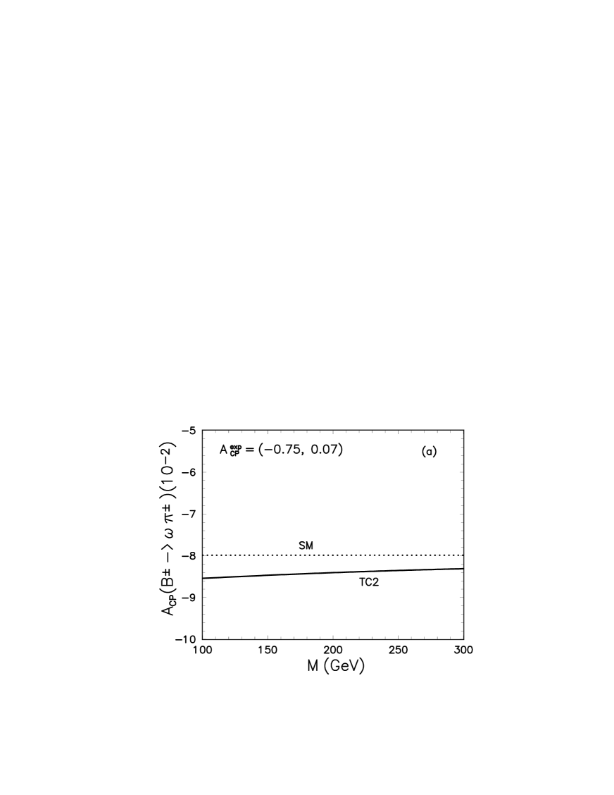
Figure 11: Same as Fig.10 but for decay $(B^{\pm}\to\omega\pi^{\pm})$. The $90\%C.L.$ allowed region from CLEO is ${\cal A}_{CP}=[-0.75,0.07]$.

It is easy to see that the CP-violating asymmetries of all five decay modes studied are small in size in both the SM and TC2 model, and well consistent with the CLEO data. For all five decay modes, the new physics corrections are also small: which will change the SM predictions by about $20\%$. Fig.10 and Fig.11 show the mass and $N_{c}^{eff}$ dependence for $B^{\pm}\to K^{\pm}\eta^{\prime}$ and $B^{\pm}\to\omega\pi^{\pm}$ in the SM (the dots lines or curves) and TC2 model (the solid curves)

From the theoretical predictions and the CLEO measurements as given in tables 9-15, the following general features about the CP-violating asymmetry of charmless hadronic B meson decays under study in this paper can be understood:

• The CP-violating asymmetries depend weakly on whether we use the BSW or LQQSR form factors. The inclusion of NP contributions does not change this feature.

• The $m_{\tilde{\pi}}$ dependence of ${\cal A}_{CP}$ is weak: $\delta{\cal A}_{CP}$ is about $\pm 15\%$ as one varies $m_{\tilde{\pi}}$ in the range $100{\rm GeV}\leq m_{\tilde{\pi}}\leq 300{\rm GeV}$.

• For twenty $B\to PP$ decays, the new physics corrections to ${\cal A}_{CP}$ are generally small or moderate in magnitude. The largest correction is about $-30\%$ for the decay $B^{\pm}\to K^{\pm}\pi^{0}$, and about $\pm 20\%$ for decay modes $\shortstack{{\tiny(\rule[0.86108pt]{5.0pt}{0.28453pt})} \\ [-.7ex] $B^{0}$}\to\pi^{+}\pi^{-},\pi^{0}\eta,K^{+}\pi^{-},K^{0}\bar{K}^{0}$ and $B^{+}\to K^{0}\pi^{+},K^{0}\bar{K}^{0}$. For four class-II $B\to\eta\eta^{(^{\prime})},\eta^{\prime}\eta^{\prime}$ and $\pi^{0}\pi^{0}$ decays, they have large CP violating asymmetries ( around $\pm 50\%$), but unfortunately also have strong $N_{c}^{eff}$-dependence in both the SM and TC2 model.

• For $B\to PV$ decays, however, the NP corrections to ${\cal A}_{CP}$ can be rather large for many decay modes, as illustrated in Table 13. For class-I-4 decay $B^{0}/\bar{B}^{0}\to\rho^{+}\pi^{-}/\rho^{-}\pi^{+}$, the new physics correction is $(60\sim 100)\%$ for $N_{c}^{eff}=2-\infty$. For decay $B^{+}\to K^{*+}\bar{K}^{0}$ the correction can even reaches a factor of 20 for $N_{c}^{eff}=2$ due to strong interference between the contributions from the $W-$penguin and new charged-scalar penguins.

• For most class-I, III and IV decays, the $N_{c}^{eff}$-dependence and $k^{2}$-dependence of $\delta{\cal A}_{CP}$ are weak. For most class-V decays, however, the $N_{c}^{eff}$-dependence of $\delta{\cal A}_{CP}$ is strong.

• For most decay modes considered here, the new physics corrections on ${\cal A}_{CP}$ in the TC2 model are still much smaller than existed theoretical uncertainties, and therefore will be masked by the later. Low experimental statistics and large theoretical uncertainties together prevent us from testing the TC2 model through the studies of CP-violating asymmetries at present.

According to relevant studies [59] for these decay modes, we know that the FSI may provide a new strong phase and therefore enhance ${\cal A}_{CP}$ to a level $20\%-40\%$, new physics with new large phases may also increase the ${\cal A}_{CP}$ to a level $40\%-60\%$. Although there is still no evidence for direct CP violation in B system, the CLEO measurements ruled out large part of the parameter space for ${\cal A}_{CP}$. The key problem is that the measurements are currently statistics limited.

6 Summary and discussions

In this paper, we calculated the new physics contributions to the branching ratios and CP-violating asymmetries of two-body charmless hadronic B meson decays $B\to PP,PV$ in the TC2 model by employing the NLO effective Hamiltonian with generalized factorization. We will present the calculation for the new physics effects on ${\cal B}(B\to VV)$ and ${\cal A}_{CP}(B\to VV)$ in a forthcoming paper[60]

We firstly evaluate analytically all strong and electroweak charged-scalar penguin diagrams in the quark level processes $b\to sV^{*}$ with $V=\gamma,gluon,\;Z$, extract out the corresponding Inami-Lim functions $C_{0}^{TC2},D_{0}^{TC2},E_{0}^{TC2}$ and $C_{g}^{TC2}$ which describe the NP contributions to the Wilson coefficients $C_{i}(M_{W})$ ($i=3-10$) and $C_{g}(M_{W})$, combine these new functions with their SM counterparts, run all Wilson coefficients from the high energy scale $\mu\approx O(M_{W})$ down to the lower energy scale $\mu=O(m_{b})$ by using the QCD renormalization equations, find the effective Wilson coefficients $C_{i}^{eff}$, and finally calculate the branching ratios and CP-violating asymmetries after inclusion of NP contributions in the TC2 model.

In section 4, we calculated the branching ratios for fifty seven $B\to PP,PV$ decays in the SM and TC2 model, presented the numerical results in tables (3-8) and displayed the $m_{\tilde{\pi}}$ and $N_{c}^{eff}$-dependence of several interesting decay modes in Figs.(2-9). From these tables and figures, the following conclusions can be reached:

• The theoretical predictions in the TC2 model for all fifty seven decay modes under study are well consistent with the experimental measurements and upper limits within one or two standard deviations.

• The theoretical uncertainties induced by varying $k^{2}$, $\eta$ and $m_{\tilde{\pi}}$ are moderate within the range of $k^{2}=m_{b}^{2}/2\pm 2GeV^{2}$, $\eta=0.34\pm 0.08$ and $m_{\tilde{\pi}}=200\pm 100$ GeV. The dependence on whether we use the BSW or LQSSR form factors are also weak. The $N_{c}^{eff}-$dependence vary greatly for different decay modes.

• For most $B\to PP$ decay channels, the NP effects $\delta{\cal B}$ are large in size and insensitive to the variations of the effective number of colors $N_{c}^{eff}$. For many $B\to PV$ decays, however, $\delta{\cal B}$ are sensitive to the variations of $N_{c}^{eff}$. It seems that the $B\to K\pi$ and $B\to K\eta^{\prime}$ decay channels are good places to test the TC2 model.

• For most class-II, IV and V decay channels, such as $B\to\eta\eta^{(^{\prime})}$, $B\to K\pi$,$B\to K\eta^{\prime}$, $etc,$ the NP enhancements to the decay rates can be rather large, from $~{}30\%$ to $~{}100\%$ $w.r.t$ the SM predictions. So large enhancements will be measurable when enough B decay events accumulated at B factories in the forthcoming years.

• For most decay modes, both new gluonic and electroweak penguins contribute effectively.

• For $B\to K\eta^{\prime}$ decays, the new physics enhancements are significant, $\sim 50\%$, and insensitive to the variations of $k^{2}$, $\eta$, $m_{\tilde{\pi}}$ and $N_{c}^{eff}$ within considered parameter space. The theoretical predictions for ${\cal B}(B\to K\eta^{\prime})$ become now consistent with the CLEO data due to the inclusion of new physics effects in the TC2 model.

In section 5, we calculated the CP-violating asymmetries ${\cal A}_{CP}$ for $B\to PP,PV$ decays in the SM and TC2 model, presented the numerical results in tables (9-14) and displayed the $m_{\tilde{\pi}}$ and $N_{c}^{eff}$-dependence of ${\cal A}_{CP}$ for decays $B^{\pm}\to K^{\pm}\eta^{\prime},\omega\pi^{\pm}$ in Figs.(10,11). In this paper, the possible effects of FSI on ${\cal A}_{CP}$ are neglected. From those tables and figures, the following conclusions can be drawn:

• Although there is no new weak phase introduced in TC2 model, the CP-violating asymmetries ${\cal A}_{CP}$ can still be changed through the interference between the ordinary tree/penguin amplitudes in the SM and the new strong and electroweak penguin amplitudes in TC2 model.

• The CP-violating asymmetries depend weakly on whether we use the BSW or LQQSR form factors in calculations in both the SM and TC2 model.

• For most $B\to PP$ decays, $\delta{\cal A}_{CP}$ are generally small or moderate in magnitude ( $10\%-30\%$ ), and insensitive to the variation of $m_{\tilde{\pi}}$ and $N_{c}^{eff}$. But the four class-II decay modes $\shortstack{{\tiny(\rule[0.86108pt]{5.0pt}{0.28453pt})} \\ [-.7ex] $B^{0}$}\to\pi^{0}\pi^{0},\eta^{(^{\prime})}\eta^{(^{\prime})}$ have strong $N_{c}^{eff}$-dependence in both the SM and TC2 model.

• For $B\to PV$ decays, however, $\delta{\cal A}_{CP}$ can be rather large for many decay modes. For decay $B^{0}/\bar{B}^{0}\to\rho^{+}\pi^{-}/\rho^{-}\pi^{+}$, the new physics correction is $(60-100)\%$ for $N_{c}^{eff}=2-\infty$. For decay $B^{+}\to K^{*+}\bar{K}^{0}$ the correction can even reaches a factor of 20 for $N_{c}^{eff}=2$. For most class-I, III and IV decays, the $N_{c}^{eff}$-dependence and $k^{2}$-dependence of $\delta{\cal A}_{CP}$ are weak. For most class-V decays, however, the $N_{c}^{eff}$-dependence of $\delta{\cal A}_{CP}$ is strong.

• For the measured five decay modes $B\to K\pi,K\eta^{\prime},\omega\pi$, the new physics effects is only about $-20\%$ w.r.t the SM predictions. The theoretical predictions for these five decay modes in the SM and TC2 model are well consistent with the CLEO measurements.

Appendix A: Input parameters

In this appendix we present relevant input parameters. We use the same set of input parameters for the quark masses, decay constants, Wolfenstein parameters and form factors as [12].

• Input parameters of electroweak and strong coupling constant, gauge boson masses, B meson masses, light meson masses, $\cdots$, are as follows (all masses in unit of GeV )[12, 42]

  $$\alpha_{em} = 1/128,\;\alpha_{s}(M_{Z})=0.118,\;\sin^{2}\theta_{W}=0.23,\;G_{F}=1.16639\times 10^{-5}(GeV)^{-2},$$

  $$M_{Z} = 91.187,\;M_{W}=80.41,\;m_{B_{d}^{0}}=m_{B_{u}^{\pm}}=5.279,\;m_{\pi^{\pm}}=0.140,\;$$

  $$m_{\pi^{0}} = 0.135,\;m_{\eta}=0.547,\;m_{\eta^{\prime}}=0.958,\;m_{\rho}=0.770,\;m_{\omega}=0.782,$$

  $$m_{\phi} = 1.019,\;m_{K^{\pm}}=0.494,\;m_{K^{0}}=0.498,\;m_{K^{*\pm}}=0.892,\;m_{K^{*0}}=0.896,$$

  $$\tau(B_{u}^{\pm}) = 1.64ps,\;\tau(B_{d}^{0})=1.56ps,$$ (139)

• For the elements of CKM matrix, we use Wolfenstein parametrization, and fix the parameters $A,\lambda,\rho$ to their central values, $A=0.81,\;\lambda=0.2205,\;\rho=0.12$ and varying $\eta$ in the range of $\eta=0.34\pm 0.08$.

• We firstly treat the internal quark masses in the loops in connection with the function $G(x_{i},z)$ as constituent masses,

  $$m_{b}=4.88GeV,\;m_{c}=1.5GeV,\;m_{s}=0.5GeV,\;m_{u}=m_{d}=0.2GeV.$$ (140)

  Secondly, we will use the current quark masses for $m_{i}$ ($i=u,d,s,c,b$) which appear through the equation of motion when working out the hadronic matrix elements. For $\mu=2.5GeV$, one finds[12]

  $$m_{b}=4.88GeV,\;m_{c}=1.5GeV,m_{s}=0.122GeV,\;m_{d}=7.6MeV,\;m_{u}=4.2MeV.$$ (141)

  For the mass of heavy top quark we also use $m_{t}=\overline{m_{t}}(m_{t})=168GeV$.

• For the decay constants of light mesons, the following values will be used in the numerical calculations (in the units of MeV):

  $$f_{\pi}=133,\;f_{K}=158,\;f_{K^{*}}=214,\;f_{\rho}=210,\;f_{\omega}=195,\;f_{\phi}=233,\;$$

  $$f^{u}_{\eta}=f^{d}_{\eta}=78,\;f^{u}_{\eta^{\prime}}=f^{d}_{\eta^{\prime}}=68,\;f^{c}_{\eta}=-0.9,\;f^{c}_{\eta^{\prime}}=-0.23,$$

  $$f^{s}_{\eta}=-113,\;f^{c}_{\eta^{\prime}}=141,$$ (142)

  where $f^{u}_{\eta^{(^{\prime})}}$ and $f^{s}_{\eta^{(^{\prime})}}$ have been defined in the two-angle-mixing formalism with $\theta_{0}=-9.1^{\circ}$ and $\theta_{8}=-22.2^{\circ}$[61] For more details about the mixings between $\eta$ and $\eta^{\prime}$, one can see [61, 13].

Appendix B: Form factors

• The form factors at the zero momentum transfer in the Baner, Stech and Wirbel (BSW) [15] model have been collected in Table 2 of ref.[12]. For the convenience of the reader we list them here:

  $$F_{0}^{B\pi}(0)=0.33,\;F_{0}^{BK}(0)=0.38,\;F_{0}^{B\eta}(0)=0.145,\;F_{0}^{B\eta^{\prime}}(0)=0.135,$$

  $$A_{0,1,2}^{B\rho}(0)=A_{0,1,2}^{B\omega}(0)=0.28,\;A_{0}^{BK^{*}}(0)=0.32,\;A_{1,2}^{BK^{*}}(0)=0.33,$$

  $$V^{B\rho}(0)=V^{B\omega}(0)=0.33,\;V^{BK^{*}}(0)=0.37.$$ (143)

• In the LQQSR approach, the form factors at zero momentum transfer being used in our numerical calculations are [12],

  $$F_{0}^{B\pi}(0)=0.36,\;F_{0}^{BK}(0)=0.41,\;F_{0}^{B\eta}(0)=0.16,\;F_{0}^{B\eta^{\prime}}(0)=0.145,$$

  $$\{A_{0},A_{1},A_{2},V\}(B\to\rho)=\{0.30,0.27,0.26,0.35\},$$

  $$\{A_{0},A_{1},A_{2},V\}(B\to K^{*})=\{0.39,0.35,0.34,0.48\},$$

  $$\{A_{0},A_{1},A_{2},V\}(B\to\omega)=\{0.30,0.27,0.26,0.35\}.$$ (144)

• The form factors $F_{0,1}(k^{2}),$ $A_{0,1,2}(k^{2})$ and $V(k^{2})$ were defined in ref.[15] as

  $$F_{0}(k^{2}) = \frac{F_{0}(0)}{1-k^{2}/m^{2}(0^{+})},\ \ F_{1}(k^{2})=\frac{F_{1}(0)}{1-k^{2}/m^{2}(1^{-})},$$

  $$A_{0}(k^{2}) = \frac{A_{0}(0)}{1-k^{2}/m^{2}(0^{-})},\ \ A_{1}(k^{2})=\frac{A_{1}(0)}{1-k^{2}/m^{2}(1^{+})},$$

  $$A_{2}(k^{2}) = \frac{A_{2}(0)}{1-k^{2}/m^{2}(1^{+})},\ \ V(k^{2})=\frac{V(0)}{1-k^{2}/m^{2}(1^{-})}.$$ (145)

• The pole masses being used to evaluate the $k^{2}$-dependence of form factors are,

  $$\{m(0^{-}),m(1^{-}),m(1^{+}),m(0^{+})\} = \{5.2789,5.3248,5.37,5.73\}$$ (146)

  for $\bar{u}b$ and $\bar{d}b$ currents. And

  $$\{m(0^{-}),m(1^{-}),m(1^{+}),m(0^{+})\} = \{5.3693,5.41,5.82,5.89\}$$ (147)

  for $\bar{s}b$ currents.

Figure 1: Typical self-energy and penguin diagrams for the quark level decays $b\to(s,d)V^{*}$ ($V=\gamma,Z^{0},g$), with $W^{\pm}$ (internal wave lines) and charged Pseudo-scalar exchanges (internal dash lines) in the SM and TC2 model. The internal quarks are the upper type quark $u,c$ and $t$.

Figure 2: Plots of branching ratios of $B\to K^{+}\pi^{0}$ decay versus $m_{\tilde{\pi}}$ and $1/N_{c}^{eff}$ in the SM and TC2 model. For (a) and (b), we set $N_{c}^{eff}=2$ and $m_{\tilde{\pi}}=200$GeV, respectively. The short-dashed line and solid curve show the branching ratio in the SM and TC2 model, respectively. The dots band corresponds to the CLEO data with $2\sigma$ errors: ${\cal B}(B\to K^{+}\pi^{0})=(11.6^{+6.6}_{-6.0})\times 10^{-6}$.

Figure 3: Same as Fig.2 but for the case of $B\to K^{+}\pi^{-}$ decay mode. The dots band corresponds to the CLEO data with $2\sigma$ errors: ${\cal B}(B\to K^{+}\pi^{-})=(17.2^{+5.6}_{-5.4})\times 10^{-6}$.

Figure 4: Same as Fig.2 but for the case of $B\to K^{0}\pi^{+}$ decay mode. The dots band corresponds to the CLEO data with $2\sigma$ errors: ${\cal B}(B\to K^{0}\pi^{+})=(18.2^{+9.8}_{-8.6})\times 10^{-6}$.

Figure 5: Same as Fig.2 but for the case of $B\to K^{0}\pi^{0}$ decay mode. The dots band corresponds to the CLEO data with $1\sigma$ error: ${\cal B}(B\to K^{0}\pi^{0})=(14.6^{+6.4}_{-6.1})\times 10^{-6}$.

Figure 6: Plots of branching ratios of decays $B^{+}\to K^{+}\eta^{\prime}$ versus $m_{\tilde{\pi}}$ and $1/N_{c}^{eff}$ in the SM and TC2 model. For (a) and (b), we set $N_{c}^{eff}=3$ and $m_{\tilde{\pi}}=200$GeV, respectively. The short-dashed line ( solid curve ) shows ${\cal B}(B^{+}\to K^{+}\eta^{\prime})$ in the SM ( TC2 model ). The dots band corresponds to the CLEO data with $2\sigma$ errors: ${\cal B}(B^{+}\to K^{+}\eta^{\prime})=(80^{+24}_{-22})\times 10^{-6}$.

Figure 7: Same as Fig.6 but for $B^{0}\to K^{0}\eta^{\prime}$ decay. The dots band corresponds to the CLEO data with $2\sigma$ errors: ${\cal B}(B^{0}\to K^{0}\eta^{\prime})=(89^{+40}_{-36})\times 10^{-6}$.

Figure 8: Plots of ${\cal B}(B^{+}\to K^{*+}\eta)$ versus $m_{\tilde{\pi}}$ and $1/N_{c}^{eff}$ in the SM and TC2 model. For (a) and (b), we set $N_{c}^{eff}=3$ and $m_{\tilde{\pi}}=200$GeV, respectively. The dot-dashed line shows the SM prediction, while the short-dashed and solid curve refer to the ratios with the inclusion of contributions induced by new gluonic penguins and both new gluonic and electroweak penguins, respectively. The upper band corresponds to the CLEO data with $1\sigma$ error: ${\cal B}(B^{+}\to K^{*+}\eta)=(26.4^{+10.2}_{-8.8})\times 10^{-6}$.

Figure 9: Same as Fig.(8), but for decay ${\cal B}(B^{0}\to K^{*0}\eta)$. The upper band corresponds to the CLEO data with $1\sigma$ error: ${\cal B}(B^{0}\to K^{*0}\eta)=(13.8^{+5.7}_{-4.9})\times 10^{-6}$.

Figure 10: Plots of CP-violating asymmetries ${\cal A}_{CP}$ $vs$ $m_{\tilde{\pi}}$ and $1/N_{c}^{eff}$ for decay $(B^{\pm}\to K^{\pm}\eta^{\prime})$. For (a) and (b) we set $N_{c}^{eff}=3$ and $m_{\tilde{\pi}}=200$ GeV, respectively. The $90\%C.L.$ allowed region from CLEO is ${\cal A}_{CP}=[-0.17,0.23]$.

References

- [1] P.F. Harrison and H.R. Quinn, Editors, The BaBar Physics Book, SLAC-R-504, 1998.
- [2] M.T. Cheng et al., Belle collaboration, KEK-Report 94-2; F. Takasaki, hep-ex/9912004; P.Eerola, Nucl.Instrum.Meth. A446, 384(2000).
- [3] R. Fleischer and J. Matias, Phys.Rev.D61, 074004(2000).
- [4] M. Misiak, S.Pokorski and J.Rosiek, inHeavy Flavor II, eds. A.J.Buras and M. Lindner( World Scientific, Singapore, 1998), p.795; S. Baek and P. Ko, Phys.Rev.Lett. 83, 488 (1999); M. Ciuchini, E. Franco, G. Martinelli, A. Masiero and L. Silerstrini, Phys.Rev.Lett. 79, 978 (1997).
- [5] D. Atwood and A. Soni, Phys.Rev.Lett. 81, 3324(1999); D. Atwood and A. Soni, Phys.Rev. D59, 013007 (1999); D. Bowser-Chao, D. Chang and W.Y. Keung, Phys.Rev.Lett. 81, 2028 (1999).
- [6] Y.L. Wu and L. Wolfenstein, Phys.Rev.Lett. 73, 1762 (1994); L. Wolfenstein and Y.L. Wu, Phys.Rev.Lett. 73, 2809 (1994); K. Huitu, D.X. Zhang, C.D. Lü and P. Singer, Phys.Rev.Lett. 81,4313 (1998); Y.F. Zhou, Y.L. Wu, Mod.Phys.Lett. A15, 185 (2000); C.S. Huang, W. Liao and Q.S. Yan, Phys.Rev. 59, 011701 (1999); Y.L. Wu, Y.F. Zhou, Phys.Rev. D61, 096001 (2000).
- [7] T.M. Aliev and E.O. Iltan, Phys.Rev. D58, 095014 (1998); T.M. Aliev, G. Hiller and E.O. Iltan, Nucl.Phys. B515, 321(1998); K. Kiers A. Soni and G.H. Wu, Phys.Rev. D59, 096001 (1999); E.O. Iltan, Phys.Rev. D60, 034023 (1999).
- [8] C.D. Lü and Z.J. Xiao, Phys.Rev. D53, 2529(1996); B. Balaji, Phys.Rev. D53, 1699 (1996); G.R. Lu, C.X. Yue, Y.G. Cao, Z.H. Xiong and Z.J. Xiao, Phys. Rev. D54, 5647 (1996); G.R. Lu, Z.H. Xiong and Y.G. Cao, Nucl.Phys. B487, 43(1997); G.R. Lu, Z.J. Xiao, H.K. Guo and L.X. Lü, J. Phys. G25, L85 (1999).
- [9] Z.J. Xiao, C.S. Li and K.T. Chao, Phys.Lett. B473, 148(2000); Z.J. Xiao, C.S. Li and K.T. Chao, Phys.Rev. D62, 094008(2000).
- [10] H. Simma and D. Wyler, Phys.Lett. B272, 395 (1991); G. Kramer, W.F. Palmer and H. Simma, Nucl.Phys. B428, 77(1994); Z.Phys. C66, 429(1995); R. Fleischer, Phys.Lett. B321, 259(1994); Z.Phys. C62, 81(1994); G. Kramer and W.F. Palmer, Phys.Rev. D52, 6411(1995); N.G. Deshpande and X.G. He, Phys.Lett. B336, 471(1994); G. Kramer, W.F. Palmer and Y.L. Wu, Commun.Theor.Phys. 27, 457(1997); C.-W. Chiang and L. Wolfenstein, Phys. Rev. D61, 074031(2000); T. Muta, A. Sugamoto, M.Z. Yang, Y.D. Yang, Phys.Rev. D62, 094020(2000).
- [11] D. Du and L. Guo, Z.Phys. C75, 9(1997); D. Du and L. Guo, J. Phys. G23, 525(1997).
- [12] A. Ali, G. Kramer and C.D. Lü, Phys.Rev. D58, 094009(1998).
- [13] A. Ali, C. Greub, Phys.Rev D57, 2996 (1998); A. Ali, J. Chay, C. Greub and P. Ko, Phys.Lett. B424, 161(1998).
- [14] Y.H. Chen, H.-Y. Cheng, B. Tseng and K.C. Yang, Phys.Rev. D60, 094014(1999).
-
[15]
M. Bauer and B. Stech, Phys.Lett. B152, 380 (1985);
M. Bauer, B. Stech and M. Wirbel, Z. Phys. C29, 637 (1985); ibid, C34, 103 (1987). - [16] H.-Y. Cheng, Phys.Lett. B335, 428(1994); B395, 345(1997); H.-Y. Cheng and B.Tseng, Phy.Rev. D58, 094005 (1998).
- [17] A.J. Buras, L. Silvestrini, Nucl.Phys. B548, 293(1999).
- [18] H.-Y. Cheng, Hsiang-nan Li and K.C. Yang, Phys.Rev. D60, 094005(1999).
- [19] M. Bishai et al., CLEO Collaboration, CLEO CONF 99-13, hep-ex/9908018; S.J. Richichi et al., CLEO Collaboration, CLEO CONF 99-12, hep-ex/9908019; T.E. Coan et al., CLEO Collaboration, CLEO CONF 99-16, hep-ex/9908029; Y. Kwon et al., CLEO Collaboration, CLEO CONF 99-14, hep-ph/9908039.
- [20] S.J. Richichi et al., CLEO Collaboration, Phys.Rev.Lett. 85, 520(2000);
- [21] D. Cronin-Hennessy et al., CLEO Collaboration, Phys.Rev.Lett. 85, 515(2000); C.P. Jessop et al., CLEO Collaboration, CLEO 99-19, hep-ex/0006008.
- [22] S. Chen et al., CLEO Collaboration, Phys.Rev.Lett. 85, 525(2000); J. O’Neill, CLEO Collaboration, CLEO Talk 00-1; W. Sun, CLEO Collaboration, CLEO Talk 00-8; V. Frolov, CLEO Collaboration, CLEO Talk 00-22.
- [23] For a summary of recent CLEO results, one can see: D. Jaffe, Talk Presented at BNL Particle Physics Seminar, 20 April, 2000, CLEO-Talk 00-10.
- [24] B. Aubert et al.,, BaBar Collaboration, paper submmitted to ICHEP’2000, Osaka, Japan, 27 Jul - 2 Aug, 2000, BaBar-Conf-00/14; J. Olsen, BaBar Cllaboration, talk given at DPF’2000, Columbus Ohino, USA, Aug. 2000, BaBar-talk-00/27.
- [25] A. Abashian et al., Belle Collaboration, talks given at ICHEP’2000, Osaka, Japan, 27 Jul - 2 Aug, 2000, Conf0005, Conf-0006, Conf0007;
- [26] A. Ali, G. Kramer and C.D. Lü, Phys.Rev. D59, 014005(1999).
- [27] G. Buchalla, A.J. Buras and M.E. Lautenbacher, Rev.Mod.Phys. 68, 1125(1996).
- [28] A.J. Buras and R. Fleischer, in Heavy Flavor II, ed. A.J.Buras and M.Lindner (World Scientific, Singapore, 1998), p.65; A.J. Buras, in Probing the Standard Model of Paticle Interactions, ed. F.David and R.Gupta, 1998 Elsevier Science B.V., hep-ph/9806471.
- [29] H.J.Lipkin, hep-ph/0009241.
- [30] C.T. Hill, Phys. Lett. B345, 483(1995);
- [31] For more details about TC2 models and experimental constraints, see K. Lane, presented at the 28th International Conference on High Energy Physics, Warsaw (July 1996), ICHEP 96:367-378.
- [32] S. Weinberg, Phys. Rev. D13, 974(1976); D19, 1277(1979); L.Susskind, ibid, D20, 2619(1979).
- [33] E. Farhi and L.Susskind, Phys.Rev. D20, 3404(1979).
- [34] G. Buchalla, G. Burdman, C.T. Hill and D. Kominis, Phys.Rev.D53, 5185(1996);
- [35] D. Kominis, Phys. Lett. B 358, 312(1995).
- [36] G. Burdman, D. Kominis, Phys. Lett. B403, 101(1997); G. Burdman, Phys. Lett. B409, 443(1997);
- [37] E. Eichten, I. Hinchliffe, K. Lane and C. Quigg, Rev.Mod.Phys. 56, 579 (1984); Phys. Rev. D34, 1547(1986); E. Eichten and K. Lane, Phys.Lett. B327, 129(1994).
- [38] Z.J.Xiao, L.X. Lü, H.K. Guo and G.R. Lu, Eur.Phys. J.C7, 487(1999).
- [39] J. Ellis, M.K. Gaillard, D.V. Nanopoulos and P. Sikivie, Nucl.Phys. B182,505(1981).
- [40] K. Lane, Phys. Rev. D54, 2204(1996).
- [41] Z.J. Xiao, C.S. Li and K.T. Chao, Eur. Phys. J. C10, 51(1999).
- [42] Particle Data Group, C. Caso et al., Eur. Phys. J. C3,1(1998).
- [43] T. Inami and C.S. Lim, Prog.Theor.Phys. 65, 297(1981).
- [44] R. Fleischer, Z.Phys.C58, 483(1993).
- [45] H.-Y. Cheng and K.C. Yang, Phys.Rev. D62, 054029(2000).
- [46] S.A. Abel, W.N. Cottinggham and I.B. Whittingham, Phys.Rev. D58, 073006(1998).
- [47] M. Bander, G. Silverman and A. Soni, Phys.Rev.Lett. 43, 242(1979);
- [48] J.M. Gérard and W.S. Hou, Phys.Rev. D43, 2909(1991).
- [49] N.G. Deshpande and J. Trampetic, Phys.Rev. D41, 2926(1990).
- [50] J. Bijnens and F. Hoogeveen, Phys.Lett. B283, 434(1992).
- [51] H.Y. Cheng, invited talk at 3rd Intern. Conf. on B Physics and CP Violation (BCONF99), Taipei, Taiwan, 3-7 Dec 1999; hep-ph/9912372.
- [52] B.H. Behrens et al., CLEO Collaboration, Phys.Rev.Lett. 80, 3710(1998).
- [53] A. Gritsan, Talk presented at UCSB, UCSD, LBNL, SLAC, CU-Boulder, March-May 2000, CLEO TALK 00-20.
- [54] H.J. Lipkin, Phsy.Lett. B433, 117(1998).
- [55] G.C. Branco, L. Lavoura and J.P. Silva, CP violation, ( Oxford University Press, 1999).
- [56] R.Waldi, Fortschr. Phys. 47, 707 (1999).
- [57] F. Abe et al., CDF Collaboration, Phsy.Rev.Lett. 81, 5513(1998).
- [58] Y.H.Chen, H.Y. Cheng and B. Tseng, Phys.Rev. D59, 074003(1998).
- [59] X.G. He, W.S. Hou and K.C. Yang, Phys. Rev. Lett. 81, 5738(1998); J. Charles, Phys.Rev. D59, 054007(1999); M. Neubert, JHEP, 9902, 014(1999); N.G. Deshpande, X.G. He, W.S. Hou and S. Pakasa, Phys.Rev.Lett. 82, 2240(1999).
- [60] Z.J. Xiao et al., in praperation.
- [61] T. Feldmann and P. Kroll, Eur.Phys.J. C5, 327 (1998).