SLAC-PUB-8703 November 2000

Randall-Sundrum Phenomenology at Linear Colliders

Abstract

The physics of the Randall-Sundrum model relevant for future linear colliders is briefly summarized. The differences between the case where Standard Model(SM) fields are on the wall and where they are in the bulk are emphasized.

Randall and Sundrum(RS)RS have recently proposed a novel approach in dealing with the hierarchy problem wherein an exponential warp factor arises from a 5-d non-factorizable geometry based on a slice of AdS₅ space. Here, two 3-branes sit at the orbifold fixed points $y=0$ (Plank brane) and $y=\pi r_{c}$ (SM or TeV brane) with equal and opposite tensions with the AdS₅ space between them. The model contains no large parameter hierarchies with $\overline{M}_{Pl}$, the 5-d Planck scale, $M_{5}$, and the AdS curvature parameter, $k$, being of qualitatively similar magnitudes. TeV scales can be generated on the brane at $y=\pi r_{c}$ if gravity is localized on the other brane and $kr_{c}\simeq 11-12$; indeed in this case the scale of physical processes on the SM brane is found to be given by $\Lambda_{\pi}=\overline{M}_{Pl}e^{-kr_{c}\pi}$ which is of order a TeV.

Such a model leads to very interesting and predictive phenomenology that can be explored in detail at collidersdhr . In the simplest scenario the SM fields are constrained to lie on the TeV brane while gravitons can propagate in the bulk in which case only two parameters are necessary to describe the model: $c=k/\overline{M}_{Pl}$, which is expected to be near though somewhat less than unity, and $m_{1}=kx_{1}e^{-kr_{c}\pi}$, which is the mass of the first graviton Kaluza-Klein excitation. The masses of the higher excitations are given by $m_{n}=m_{1}x_{n}/x_{1}$, where the $x_{n}$ are roots of the Bessel function $J_{1}(x_{n})=0$, and are thus not equally spaced. While the massless zero mode graviton couples in the usual manner as $(\overline{M}_{Pl})^{-1}$, the tower states instead couple as $\Lambda_{\pi}^{-1}$.

The most distinctive prediction of this scenario is the direct production of weak scale graviton resonances at colliders as is shown in Fig. 1 for the case of a linear collider. Note that for fixed mass the width of each resonance is proportional to $c^{2}$; for resonances beyond the first KK excitation, the width grows as $m^{3}$. This explains why resonances with large KK number tend to get smeared out into a continuum. Present searches for graviton resonances at the Tevatron as well as analyses of their indirect contributions to electroweak observables already place significant constraints on the $c-m_{1}$ plane. When combined with our theoretical prejudices the complete allowed region for the RS model is shown in Fig. 1 in comparison to the reach of the LHC. Even given some fuzziness in our prejudices it is apparent that the LHC should cover the entire RS parameter space either by discovering a graviton resonance or excluding the model.

     

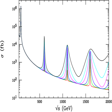
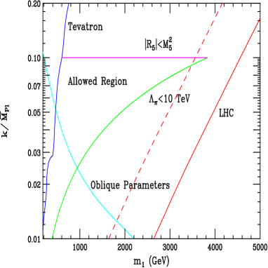
Figure 1: The left panel shows the production of KK graviton resonances in the process $e^{+}e^{-}\rightarrow\mu^{+}\mu^{-}$ assuming $m_{1}=600$ GeV for various values of $c$. The right panel shows the allowed region of the RS parameter space in comparison to the discovery region accessible to the LHC with a luminosity of 10(100)fb^-1 which lies to the left of the slanting dashed(solid) line. The Tevatron has excluded the region to the left of the irregular line on the left whereas an analysis of the oblique parameters excludes the region below the smoothly falling curve. Our theoretical prejudice that $\Lambda_{\pi}$ not be too large excludes the region below the smoothly rising curve while our similar bias that quantum effects do not dominate in the RS setup restricts $c$ to be less than $\simeq 0.1$. These last two bounds should be considered ‘soft’ in that some fuzziness should be allowed in their direct application as model constraints.

If the SM gauge fields alone are allowed to propagate in the bulk then it can be shown that the gauge KK excitations couple much more strongly to the remaining wall fields than do the zero modesdhr by a factor $\simeq\sqrt{2\pi kr_{c}}$. The exchange and mixing of these modes contribute to the electroweak observables and result in a bound $\Lambda_{\pi}>100$ TeV which is perhaps too high to claim a solution to the hierarchy problem. This strong bound can be alleviated by also placing the SM fermions in the bulk as well with the Higgs field remaining on the wall for a number of technical reasonsdhr . For simplicity and to avoid FCNC we assume that all SM fermions have an identical 5-d mass $m_{5d}=k\nu$, with $\nu$ a parameter of order unity. Specifying $\nu$ and $m_{1}$ for the graviton determines all of the KK masses with fermion excitations always more massive than gauge excitations and are approximately linear functions of $|\nu+1/2|$.

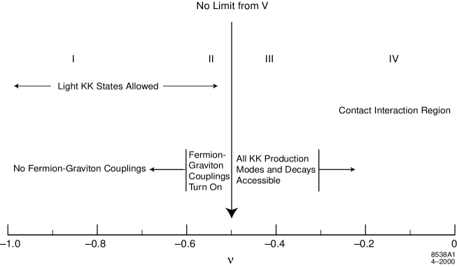
Figure 2: The descriptive phenomenology for each region of $\nu$ as discussed in the text. ‘V’ refers to the radiative corrections analysis.

The phenomenology of this version of the RS model is quite $\nu$ dependent as shown in Fig. 2. In region IV the masses of the KK states are too large for them to be produced at any planned collider and exchanges can only be probed via contact interactions as shown in Fig. 3. This region is generally disfavoured since it leads to large values of $\Lambda_{\pi}>10$ TeV. In regions II and III the KK states are sufficiently light and their couplings are such that both gauge and graviton resonances will be observable at colliders as shown in Fig. 3. In region I, the graviton KK states effectively decouple and the gauge KK coupling strengths become small in comparison to the zero modes. However the gauge KK states will still be observable as very narrow excitations at colliders as shown in Fig. 3.

Clearly future linear colliders can cover all of the possible regions allowed when the SM fields are either on or off the wall thus allowing for detailed studies of the RS model.

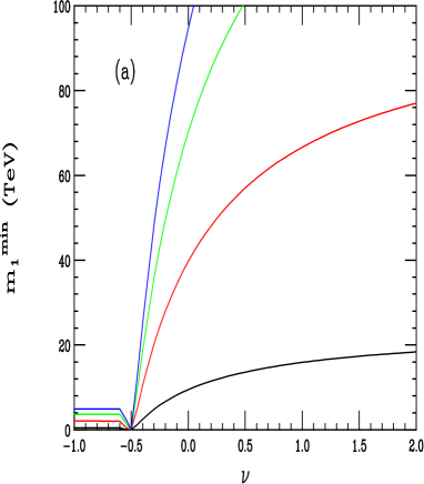
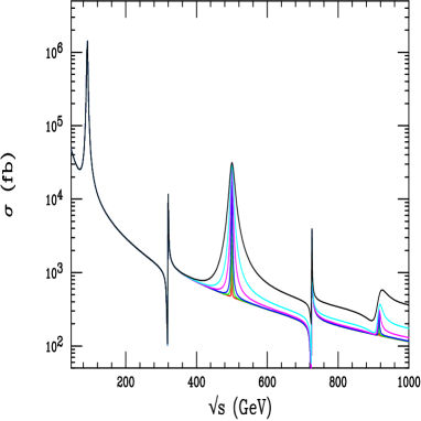
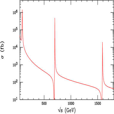
Figure 3: In the top panel is shown the contact interaction limit on the scale of the first KK exchange at lepton colliders. From top to bottom for the NLC with 500 fb^-1 and $\sqrt{s}=$1.5, 1 and 0.5 TeV and LEP II at $\sqrt{s}$=195 GeV with 1 fb^-1. In the lower left panel one sees the simultaneous production of graviton and gauge KK states typical of regions II and III via the process $e^{+}e^{-}\rightarrow\mu^{+}\mu^{-}$. In the lower right panel for region I only the gauge KK states are produced as resonances for this same process.

References

- (1) L. Randall and R. Sundrum, Phys. Rev. Lett. 83, 3370 (1999).
- (2) H. Davoudiasl, J.L. Hewett and T.G. Rizzo, Phys. Rev. Lett. 84, 2080 (2000), Phys. Lett. B473, 43 (2000) and hep-ph/0006041.