HIP-2000-59/TH
TURKU-FL-P36-00

Numerical simulations of fragmentation of the Affleck-Dine condensate

Abstract

We present numerical simulations of fragmentation of the Affleck-Dine condensate in two spatial dimensions. We argue analytically that the final state should consist of both Q-balls and anti-Q-balls in a state of maximum entropy, with most of the balls small and relativistic. Such a behaviour is found in simulations on a 100$\times$100 lattice with cosmologically realistic parameter values. During fragmentation process, we observe filament-like texture in the spatial distribution of charge. The total charge in Q-balls is found to be almost equal to the charge in anti-Q-balls and typically orders of magnitude larger than charge asymmetry. Analytical considerations indicate that, apart from geometrical factors, the results of the simulated two dimensional case should apply also to the fully realistic three dimensional case.

¹kari.enqvist@helsinki.fi; ²asko.jokinen@helsinki.fi; ³tuomas@maxwell.tfy.utu.fi;
⁴vilja@newton.tfy.utu.fi

1 Introduction

The Minimal Supersymmetric Standard Model (MSSM) has several flat directions where the scalar potential is nearly identically zero [2]. During inflation, squark and slepton fields will fluctuate freely along the flat directions, forming Affleck-Dine (AD) -condensates [3]. The state of lowest energy, however, is not the AD-condensate but a non-topological soliton, the Q-ball [4, 5], which carries a non-zero baryonic (B-ball) or leptonic (L-ball) charge. The instability is induced by the spatial perturbations [6, 7] which are naturally present in the condensate because of quantum fluctuations during inflation. The fragmentation process and the properties of the resulting Q-balls depend on SUSY breaking: if gauge mediated, Q-balls will be large and completely stable [6, 8] and form along every flat direction and could be detectable even today [10], whereas if SUSY breaking is gravity mediated, Q-balls will be unstable [7, 11] but long-lived enough to have a host of interesting cosmological consequences [11, 12]. In the gravity mediated case the formation of Q-balls is also a generic feature in all but few flat directions [13].

Fragmentation of the AD-condensate involves highly non-linear dynamics and is therefore quite complicated [14, 15]. The condensate lumps must somehow loose the extra energy when settling down to a Q-ball configuration. This they may do by radiating out quanta of AD-scalars or smaller condensate lumps, but the lumps may also experience frequent collisions. Since for a fixed charge the energy of a Q-ball is also fixed, fragmentation dynamics and the final distribution of Q-balls will obviously depend on the initial energy and charge density of the condensate. In principle, this is a free parameter, although the observed baryon asymmetry can be argued to indicate a natural order of magnitude for the ratio.

In Ref. [14] the relaxation of a single spherical condensate lump was followed numerically, but sphericality is likely to be a far too constraining assumption. Moreover, the condensate fragments are not isolated but interact with each other. The general features of Q-ball collisions have been studied in Refs. [16, 17, 18]; the cross section in the gravity mediated case has been shown to depend on the relative phases of the colliding Q-balls [17]. Q-ball formation has been seen in 3-d lattice studies both in gauge mediated [19] and gravity mediated [20] cases but only for a single energy-to-charge ratio of the condensate in each case. As we will show in this paper, natural choices for the initial energy-to-charge ratio necessarily lead to a copious formation of not only Q-balls but also of anti-Q-balls, which carry a net negative charge. Such a conclusion can be reached already by relatively simple analytical arguments which assume that the condensate lump reaction rates are fast enough to drive them into a state of maximum entropy. From the resulting equilibrium distributions it then follows that the number of Q-balls is almost equal to the number of anti-Q-balls so that the total positive (negative) charge in Q-balls is typically much larger than the actual charge asymmetry. Indeed, as we shall discuss in this paper, detailed numerical simulations show this behaviour.

The paper is organized as follows. In Section 2 we derive the Q-ball and anti-Q-ball number density distributions by assuming that the condensate lumps actually equilibrate; this is shown to be a self-consistent assumption. We also show that as far as the distributions are concerned, there is no qualitative difference between two and three spatial dimensions. In Section 3 we present the results of numerical simulations of the condensate fragmentation in 2+1 dimensions. We follow the time evolution of the condensate field, show it breaking up into Q-balls and anti-Q-balls, and extract the number density distributions from the numerical data. In Section 4 we present our conclusions.

2 Distributions of Q-balls and anti-Q-balls

2.1 AD-condensate fragmentation

In the cosmological context the formation of Q-balls via fragmentation of the AD-condensate has to be characterized by taking into account the expansion of the universe. The random perturbations on the homogeneous AD-condensate field generated during de Sitter -phase of the inflation first grow linearly as long as they remain small compared to the AD-field. When these linear modes are large enough, they become non-linear mode by mode and their dynamics becomes much more complicated. During this non-linear era the actual Q-balls are formed as the system finds the energetically most favourable configuration ending up with a particular system of Q-balls and, in general, radiation.

To be able to quantify the dynamics of the Q-balls one has to specify the potential. It consists of various terms appearing from the effective field theory of the particular case. To lowest order, a generic general potential reads

$$\mbox{$$}V_{H}(\Phi)=V(\Phi)-gH^{2}|\Phi|^{2},\vspace{\undereqskip}$$ (1)

where the second term, depending on the Hubble rate $H=\dot{a}/a$, where $a(t)$ is the scale factor, originates from higher-order operators in the Kähler potential (with typically $g\sim 1$), while $V$ includes all terms of the flat direction.

Of particular interest are flat-direction potentials of the form [7]

$$\mbox{$$}V(\Phi)=m^{2}|\Phi|^{2}(1+K\log({|\Phi|^{2}\over M^{2}}))+{\lambda^{2}\over M^{2}_{Pl}}|\Phi|^{6},\vspace{\undereqskip}$$ (2)

arising in the gravity mediated SUSY breaking scenario with a d=4 flat direction, and [6]

$$\mbox{$$}V(\Phi)=m^{4}\ln\left(1+{|\Phi|^{2}\over m^{2}}\right)+{\lambda\over M^{2}_{Pl}}|\phi|^{6}\vspace{\undereqskip}$$ (3)

in the gauge mediated SUSY breaking scenario. The mass scale $m$ is given by the SUSY breaking scale; typically $m\sim{\cal O}(100){\rm\ GeV}$. We have here omitted all terms which violate the quantum number $Q$. These are surely needed for generating the net charge of the AD-condensate, but the $Q$-violating terms are negligible at the time when the condensate finally begins to fragment. Therefore we may simply assume as an initial condition that at the onset of fragmentation the AD-condensate has some non-zero initial charge $Q$.

The initial state of the AD-condensate is determined by two parameters, the energy and charge density of the condensate. For a fixed charge $Q$ the critical parameter determining the Q-ball distribution is the ratio of energy density $\rho$ to charge density $q$,

$$\mbox{$$}x(\Phi)={\rho(\Phi)\over m\,q(\Phi)}.\vspace{\undereqskip}$$ (4)

One should note that according to our assumptions the charge density is a conserved quantity whereas the energy density is not. However, a simple calculation reveals that in a matter dominated universe the energy pumped into the scalar field by gravitation is very small compared to the initial energy of the condensate, so that in practice also $\rho$ is conserved. Hence, the ratio $x$ is a good parameter to describe the system. It is clear that the larger $x$ is the more energy should be stored as radiation, kinetic energy of Q-balls, anti-Q-balls or some combination of these.

To get an impression of the general features of the Q-ball formation process, it is useful to study instabilities in both gauge and gravity mediated scenarios. By writing the AD-condensate in terms of the modulus and the phase,

$$\mbox{$$}\Phi=\phi\,e^{i\theta},\vspace{\undereqskip}$$ (5)

one can formalize the requirements for the occurrence of the instabilities $\delta\Phi$ in the model. When the Q-balls begin to form, the instability band of fluctuations in the gauge mediated case is essentially given by [19]

$$\mbox{$$}{k\over a(t)}\;\raise 1.29167pt\hbox{$<$\kern-7.5pt\raise-4.73611pt\hbox{$\sim$}}\;{m^{2}\over\phi},\vspace{\undereqskip}$$ (6)

where it is assumed that the field $\phi$ is large. This implies, that the size of the instabilities is bounded below by

$$\mbox{$$}\lambda\sim\frac{1}{k}\;\raise 1.29167pt\hbox{$>$\kern-7.5pt\raise-4.73611pt\hbox{$\sim$}}\;{|\Phi|\over a(t)m^{2}}.\vspace{\undereqskip}$$ (7)

In a cosmological context where the field is large this implies that the Q-balls will be very large. Indeed, this can be seen in the study by Kasuya and Kawasaki [19], where they establish the formation of Q-balls using 3D lattice simulations. In their simulation one can see a single large Q-ball containing virtually all of the initial charge set into the system: this Q-ball most likely forms from the perturbation first entering the lattice, i.e. the first unstable mode which fits inside the lattice. However, the most amplified mode is even larger. These considerations make the gauge mediated scenario ineffective to study on a lattice: the lattice size should be huge in order to contain the relevant modes visible already at the very beginning.

The situation is, however, different in the gravity mediated case. The instability band is characterized by

$$\mbox{$$}{k^{2}\over a^{2}}\;\raise 1.29167pt\hbox{$<$\kern-7.5pt\raise-4.73611pt\hbox{$\sim$}}\;\dot{\theta}^{2}-V^{\prime\prime},\vspace{\undereqskip}$$ (8)

which has to be positive in order to have growing modes at all. Moreover, the maximally growing mode can be identified as $(k_{max}/a)^{2}=\frac{1}{2}(\dot{\theta}^{2}-V^{\prime\prime})$ and its growth is characterized by $|\delta\Phi|\sim e^{\alpha(t)}$, where

$$\mbox{$$}\dot{\alpha}(t)={\dot{\theta}^{2}-V^{\prime\prime}\over 4\dot{\theta}}.\vspace{\undereqskip}$$ (9)

If $\dot{\theta}\simeq m$ the wave number of the maximally growing mode is $k_{max}=\sqrt{\frac{3}{2}|K|}\,a(t)\,m$ and $\dot{\alpha}=\frac{3}{8}\,|K|\,m$. This would mean that the criteria for the end of linear growth, $\left|{\delta\Phi\over\Phi}\right|\sim 1$, implies $\alpha(t)\sim\dot{\alpha}t\sim\ln\left|{\Phi(t=0)\over\delta\Phi(t=0)}\right|$ which, in the light of the simulations, is typically too small, as will become evident later. Therefore it is important to recognize that for the $x>1$ cases $\dot{\theta}(t=0)\ll m$, and hence no instabilities occur because $V^{\prime\prime}$ is typically positive. Due to the dynamics $\dot{\theta}$ begins to grow and unstable modes appear when $\dot{\theta}^{2}-V^{\prime\prime}$ changes its sign to positive. At that time, however, the rate of perturbation growth is very slow because $\dot{\alpha}$ is very small ($\dot{\theta}\sim m$). So the growth of the perturbations is very slow at first, but later the rate of growth increases and becomes much faster when the average $\dot{\theta}^{2}$ is large enough. This lengthens remarkably the time needed to enter the non-linear era of perturbation growth and pushes the actual formation of Q-balls later.

Note that when the growth of linear modes is finally speeded up, the most amplified modes are remarkably smaller than in the gauge mediated scenario. This naturally implies that the size of the largest Q-ball is much larger in the gauge mediated than in the gravity mediated scenario.

In both gauge and gravity mediated cases the unstable perturbations $\delta\Phi$ remain linear as long as they are much smaller than the background AD-condensate field $\Phi$:

$$\mbox{$$}\left|{\delta\Phi\over\Phi}\right|\ll 1.\vspace{\undereqskip}$$ (10)

On the other hand the charge density perturbations $\delta q=q(\Phi+\delta\Phi)-q(\Phi)$ are always smaller or equal than the field perturbations, i.e.

$$\mbox{$$}\left|{\delta q\over q}\right|\leq\left|{\delta\Phi\over\Phi}\right|.\vspace{\undereqskip}$$ (11)

This implies definitely that $\left|{\delta q\over q}\right|\sim 1$ indicates the end of the linear growth era of the perturbations.

2.2 Equilibrium ensembles

After fragmentation, the AD lumps are expected to interact vigorously. Gradually the field fragments will settle to the state of lowest energy by emitting and exchanging smaller fragments. If the interaction is fast enough compared with the expansion rate of the universe, a natural expectation is that the final state should consist of an equilibrium distribution of Q-balls and anti-Q-balls in a state of maximum entropy. We shall now work out the consequences of such an assumption in the case of gravity mediated Q-balls, for which the mass $M_{Q}$ is given approximately by

$$\mbox{$$}M_{Q}\approx m\,Q~{}.\vspace{\undereqskip}$$ (12)

Q-ball (anti-Q-ball) distributions $N_{+}(Q,p)$ ($N_{-}(Q,p)$) are subject to the following constrains:

$$\mbox{$$}E_{tot}=E_{+}+E_{-}~{}, E_{\pm}=\int dQ~{}dp~{}E(Q,p)~{}N_{\pm}(Q,p)~{}$$

$$Q_{tot}=Q_{+}-Q_{-}~{}, Q_{\pm}=\int dQ~{}dp~{}Q~{}N_{\pm}(Q,p)~{},\vspace{\undereqskip}$$ (13)

where $E(Q,p)\approx\sqrt{p^{2}+m^{2}Q^{2}}$ is the energy of a single Q-ball, $E_{+}$ $(E_{-})$ and $Q_{+}$ $(Q_{-})$ are the energy and charge of Q-balls (anti-Q-balls), and $E_{tot}$ and $Q_{tot}$ are respectively the total energy and charge of Q-balls and anti-Q-balls, which are equal to the corresponding values of the AD-condensate in the beginning unless significant amounts of energy and/or charge are transformed into radiation. It then follows from Eq. (2.2) that

$$\mbox{$$}E_{tot}\geq m\,(Q_{+}+Q_{-})\geq m\,Q_{tot}.\vspace{\undereqskip}$$ (14)

This condition is independent of the precise form of the Q-ball distributions. It is easy to see that the energy-to-charge ratio (see Eq. (4)) $x\geq 1$. If $x=1$, the inequalities in Eq. (14) simplify to equalities and this gives directly the Q-ball distributions

$$\mbox{$$}N_{+}(Q,p)=N_{+}(Q)~{}\delta(p)~{},\qquad N_{-}(Q,p)=0~{},\vspace{\undereqskip}$$ (15)

which means that there are no anti-Q-balls and that the Q-balls for at rest with a distribution $N_{+}(Q)$. However, this is not a realistic case. Indeed, if all the baryon asymmetry resides in Q- and anti-Q-balls, then at times earlier than $10^{-6}s$, $Q_{tot}/Q_{+}\sim\Delta B\sim 10^{-8}$. (Since $B-L$ is conserved in the MSSM, this holds also for the purely leptonic flat directions.) From Eq. (14) it then would follow that

$$\mbox{$$}x\simeq 10^{8}~{}.\vspace{\undereqskip}$$ (16)

Even if all of the baryon asymmetry were not carried by Q-balls (or rather, in this case, by B-balls), it is likely that some of it is. As a consequence, a natural expectation is $x\gg 1$.

Hence the number of Q-balls, $N_{+}$, and the number of anti-Q-balls, $N_{-}$, are approximately equal so that the total number of Q-balls is $N_{tot}\approx 2N_{+}$. Then from Eq. (2.2) it follows that

$$\mbox{$$}E_{\pm} \approx E(\bar{Q},\bar{p})~{}\int dQ~{}dp~{}N_{\pm}(Q,p)~{}\approx~{}E(\bar{Q},\bar{p})~{}N_{+}~{},$$

$$Q_{\pm} \approx \bar{Q}~{}\int dQ~{}dp~{}N_{\pm}(Q,p)~{}\approx~{}\bar{Q}~{}N_{+}~{},\vspace{\undereqskip}$$ (17)

where $E(\bar{Q},\bar{p})$ is the average energy of one Q-ball with the average charge $\bar{Q}$ and average momentum $\bar{p}$. Now the energy charge ratio of Q-balls (anti-Q-balls), $x_{+}=E_{+}/mQ_{+}~{}~{}(x_{-}=E_{-}/mQ_{-})$, determines the average momentum of Q-balls

$$\mbox{$$}\bar{p}\approx m~{}\bar{Q}~{}\sqrt{x_{\pm}^{2}-1}\;\raise 1.29167pt\hbox{$>$\kern-7.5pt\raise-4.73611pt\hbox{$\sim$}}\;0.1~{}m~{}\bar{Q}~{},\vspace{\undereqskip}$$ (18)

when $x_{\pm}\;\raise 1.29167pt\hbox{$>$\kern-7.5pt\raise-4.73611pt\hbox{$\sim$}}\;1.01$. The average velocity will then be $<v>=\bar{p}/E(\bar{Q},\bar{p})\;\raise 1.29167pt\hbox{$>$\kern-7.5pt\raise-4.73611pt\hbox{$\sim$}}\;0.1$. If Q-balls were non-relativistic, it would cause a restriction $x_{\pm}-1<0.01$, which is not natural, as will be seen later. Thus the main bulk of Q-balls, except the largest ones, may be expected to be relativistic.

Since most Q-balls are relativistic it is not surprising that the reaction rate turns out to be much larger than the Hubble rate. We find

$$\mbox{$$}\Gamma=\frac{N_{tot}}{V}<\sigma v>\approx{4\pi\rho\bar{p}R^{2}\over E(\bar{Q},\bar{p})^{2}}~{},\vspace{\undereqskip}$$ (19)

where we have approximated the cross section by the geometrical cross section with $R$ the radius of the Q-ball. The cross section actually depends on the relative phase difference between the colliding Q-balls [17] as is largest when the phases are aligned; however, the order of magnitude is that of the geometrical cross section.

When $x\gg 1$, the charge and the momenta of Q-balls and anti-Q-balls are almost the same. The reaction rate Eq. (19) is at its maximum for $\bar{p}=m\bar{Q}$ corresponding to $x_{\pm}\approx\sqrt{2}$, which is about the same as the equilibrium value. The average charge is $\bar{Q}=q_{+}V_{1}$ where $q_{+}$ is the charge density inside a Q-ball and $V_{1}$ it’s volume. Thus we can rewrite (19) as $\Gamma={3V_{1}\rho/2m\bar{Q}R}={3\rho/2mq_{+}R}$. In the dense-packing limit, $\rho\approx 2mq_{+}x_{+}\approx 2\sqrt{2}\,mq_{+}$, and hence

$$\mbox{$$}\Gamma\approx\frac{1}{R}~{}.\vspace{\undereqskip}$$ (20)

We approximate the radius of Q-balls by $R\approx|K|^{-1/2}m^{-1}$ Eq. (2) and compare this to the Hubble rate $H\sim mt_{0}/t$ to find that $\Gamma>H$ when

$$\mbox{$$}t\;\raise 1.29167pt\hbox{$>$\kern-7.5pt\raise-4.73611pt\hbox{$\sim$}}\;\frac{t_{0}}{|K|^{1/2}}\vspace{\undereqskip}$$ (21)

Since typically $|K|\sim 0.01-0.1$ [13], the reaction rate will be larger than the Hubble rate from the very beginning, and a thermal equilibrium can be expected to be reached.

Guided by these considerations, let us now find the equilibrium distributions for Q-balls in the gravity-mediated case in two and three dimensions. The one-particle partition function reads

$$\mbox{$$}Z_{1}=g\int\limits_{V_{D}}\frac{d^{D}{x}~{}d^{D}{p}}{(2\pi)^{D}}\int\limits_{-\infty}^{\infty}dQ~{}e^{-\beta E+\mu Q},\vspace{\undereqskip}$$ (22)

where $\mu$ is the chemical potential related to the charge of Q-balls. In $D$ dimensions we may integrate Eq. (22) to obtain a distribution function with respect to charge

$$\mbox{$$}Z_{1}=\int\limits_{-\infty}^{\infty}dQ~{}Z_{1}(Q)=2gV_{D}\beta\left(\frac{m}{2\pi\beta}\right)^{\frac{D+1}{2}}\int\limits_{-\infty}^{\infty}dQ~{}|Q|^{\frac{D+1}{2}}~{}e^{\mu Q}~{}K_{\frac{D+1}{2}}(\beta m|Q|)~{},\vspace{\undereqskip}$$ (23)

where $K_{n}(z)$ is the modified Bessel function. Then we may integrate Eq. (23) to obtain an expression that can be split into positive and negative charge parts:

$$\mbox{$$}Z_{1} = Z_{1}^{-}+Z_{1}^{+}$$

$$Z_{1}^{\pm} = \frac{2gV_{D}\beta m^{D+1}(D+1)!}{\pi^{\frac{D}{2}}\Gamma(\frac{D}{2}+2)}\left[\frac{F(D+2,\frac{D}{2}+1;\frac{D}{2}+2:-\frac{\beta m\pm\mu}{\beta m\mp\mu})}{(\beta m\mp\mu)^{D+2}}\right]~{},\vspace{\undereqskip}$$ (24)

where $F(a,b;c:x)$ is the hypergeometric function. For $D=2$ and $D=3$ these expressions simplify to

$$\mbox{$$}Z_{1}^{\pm} = \frac{gV_{2}}{2\pi\beta^{2}}\frac{2\beta m\mp\mu}{(\beta m\mp\mu)^{2}},~{}D=2~{};$$ (25)

$$Z_{1}^{\pm} = \frac{gV_{3}}{\pi^{2}\beta^{3}}\left[\pm\frac{\mu(5\beta^{2}m^{2}-2\mu^{2})}{2(\beta^{2}m^{2}-\mu^{2})^{2}}+\frac{3\beta^{4}m^{4}}{(\beta^{2}m^{2}-\mu^{2})^{\frac{5}{2}}}\arctan\sqrt{\frac{\beta m\pm\mu}{\beta m\mp\mu}}\right],~{}D=3.$$

The total partition function is the sum of these two terms:

$$\mbox{$$}Z_{1} = \frac{2gV_{2}\beta m^{3}}{\pi(\beta^{2}m^{2}-\mu^{2})^{2}},\qquad D=2~{};$$ (27)

$$Z_{1} = \frac{3gV_{3}\beta m^{4}}{2\pi(\beta^{2}m^{2}-\mu^{2})^{\frac{5}{2}}},\qquad D=3.\vspace{\undereqskip}$$ (28)

The grand canonical partition function is given, as usual, by

$$\mbox{$$}Z_{G}=\sum_{N=0}^{\infty}{e^{\bar{\mu}N}Z_{1}^{N}\over N!}=e^{zZ_{1}}\vspace{\undereqskip}$$ (29)

($z=e^{\bar{\mu}}$) with the energy, charge and number of Q-balls given respectively as

$$\mbox{$$}E_{tot}=-\frac{\partial\log Z_{G}}{\partial\beta};~{}~{}Q_{tot}=\frac{\partial\log Z_{G}}{\partial\mu};~{}~{}N_{tot}=\frac{\partial\log Z_{G}}{\partial\bar{\mu}}.\vspace{\undereqskip}$$ (30)

Using Eq. (23) in Eq. (30) the total energy of the Q-ball system is obtained

$$\mbox{$$}E_{tot}=mN_{tot}~{}\int\limits_{-\infty}^{\infty}dQ~{}f_{E}(Q)~{},\vspace{\undereqskip}$$ (31)

where

$$\mbox{$$}f_{E}(Q)=\frac{2}{6-D}~{}(2\pi)^{-\frac{D-1}{2}}~{}\left[1-\left(\frac{\mu}{\beta m}\right)^{2}\right]^{\frac{D}{2}+1}~{}(\beta m|Q|)^{\frac{D+3}{2}}~{}e^{\mu Q}~{}K_{\frac{D+3}{2}}(\beta m|Q|)~{}\vspace{\undereqskip}$$ (32)

is the energy distribution function per Q-ball scaled with the mass $m$. The average energies of Q-balls and anti-Q-balls are then found from Eqs. (25, LABEL:part61) to be

$$\mbox{$$}E_{\pm} = \frac{N_{tot}}{2\beta^{4}m^{3}}\frac{(\beta m\pm\mu)^{2}(3\beta^{2}m^{2}\mp 3\beta m\mu+\mu^{2})}{\beta m\mp\mu},~{}~{}D=2~{};$$ (33)

$$E_{\pm} = \frac{2N_{tot}}{\pi\beta}\Big{[}\pm\frac{\mu}{2\beta^{4}m^{4}}\frac{6\beta^{4}m^{4}-5\beta^{2}m^{2}\mu^{2}+2\mu^{4}}{\sqrt{\beta^{2}m^{2}-\mu^{2}}}$$

$$+ \frac{4\beta^{2}m^{2}+\mu^{2}}{\beta^{2}m^{2}-\mu^{2}}\arctan\sqrt{\frac{\beta m\pm\mu}{\beta m\mp\mu}}\Big{]},~{}~{}D=3.$$

The total energy is, again, the sum of positive and negative parts:

$$\mbox{$$}E_{tot}=\frac{N_{tot}}{\beta}\frac{3\beta^{2}m^{2}+\mu^{2}}{\beta^{2}m^{2}-\mu^{2}},~{}~{}D=2~{};$$ (35)

$$E_{tot}=\frac{N_{tot}}{\beta}\frac{4\beta^{2}m^{2}+\mu^{2}}{\beta^{2}m^{2}-\mu^{2}},~{}~{}D=3.\vspace{\undereqskip}$$ (36)

Similar calculations can also be repeated for charge and particle number. We get the total charge

$$\mbox{$$}Q_{tot}=N_{tot}\int\limits_{-\infty}^{\infty}dQ~{}{\rm sign}(Q)~{}f_{Q}(Q)~{},\vspace{\undereqskip}$$ (37)

where

$$\mbox{$$}f_{Q}(Q)=\frac{2~{}(2\pi)^{-\frac{D-1}{2}}}{6-D}~{}\left[1-\left(\frac{\mu}{\beta m}\right)^{2}\right]^{\frac{D}{2}+1}~{}(\beta m|Q|)^{\frac{D+3}{2}}~{}e^{\mu Q}~{}K_{\frac{D+1}{2}}(\beta m|Q|)~{}\vspace{\undereqskip}$$ (38)

is the charge distribution function per Q-ball. The positive and negative parts of the total charge are:

$$Q_{\pm}=\frac{N_{tot}}{4\beta^{3}m^{3}}\frac{(\beta m\pm\mu)^{2}(3\beta m\mp\mu)}{\beta m\mp\mu},~{}~{}D=2~{};$$ (39)

$$Q_{\pm}=\frac{N_{tot}}{3\pi}\left[\frac{8\beta^{4}m^{4}+9\beta^{2}m^{2}\mu^{2}-2\mu^{4}}{\beta^{4}m^{4}\sqrt{\beta^{2}m^{2}-\mu^{2}}}\pm\frac{30\mu}{\beta^{2}m^{2}-\mu^{2}}\arctan\sqrt{\frac{\beta m\pm\mu}{\beta m\mp\mu}}\right],~{}~{}D=3~{}.$$

(40)

The charges are defined to be positive so that the total charge is $Q_{tot}=Q_{+}-Q_{-}$. Thus

$$\mbox{$$}Q_{tot}=N_{tot}\frac{4\mu}{\beta^{2}m^{2}-\mu^{2}},\qquad D=2~{};$$ (41)

$$Q_{tot}=N_{tot}\frac{5\mu}{\beta^{2}m^{2}-\mu^{2}},\qquad D=3~{}.\vspace{\undereqskip}$$ (42)

Moreover, the relative number distribution function of Q-balls fulfilling condition

$$\mbox{$$}\beta m\int\limits_{-\infty}^{\infty}dQ~{}f_{N}(Q)=1\vspace{\undereqskip}$$ (43)

reads now

$$\mbox{$$}f_{N}(Q)=\frac{2(2\pi)^{-\frac{D-1}{2}}}{6-D}~{}\left[1-\left(\frac{\mu}{\beta m}\right)^{2}\right]^{\frac{D}{2}+1}~{}(\beta m|Q|)^{\frac{D+1}{2}}~{}e^{\mu Q}~{}K_{\frac{D+1}{2}}(\beta m|Q|)~{}.\vspace{\undereqskip}$$ (44)

Finally, the number of positive and negative charge Q-balls is then found to be

$$\mbox{$$}N_{\pm} = \frac{N_{tot}}{4\beta^{3}m^{3}}(2\beta m\mp\mu)(\beta m\pm\mu)^{2},\ D=2\;;$$ (45)

$$N_{\pm} = \frac{N_{tot}}{\pi}\left[\pm\frac{\mu(5\beta^{2}m^{2}-2\mu^{2})}{3\beta^{4}m^{4}}\sqrt{\beta^{2}m^{2}-\mu^{2}}+2\arctan\sqrt{\frac{\beta m\pm\mu}{\beta m\mp\mu}}\right],\ D=3\;.$$

We have plotted the charge and number distribution functions for $-10\leq\beta mQ\leq 10$ in $D=2$ and $D=3$ for $\mu=0,~{}0.1\beta m$ in Figs. 2 and 2. The energy distribution function has a behaviour which is qualitative similar to the number distribution function. The total numbers of Q-balls and anti-Q-balls in $D=2$ and $D=3$ are plotted in Fig. 4 for $1\leq x\leq 30$. When $x\geq 30$ there are almost equal numbers of Q-balls and anti-Q-balls.

Figure 1: Charge distributions of Q-balls for $\mu=0$ (solid lines) and $\mu=0.1\beta m$ (dashed lines) in $D=2$ (thin lines) and $D=3$ (thick lines).

Figure 2: Number distributions of Q-balls for $\mu=0$ (solid lines) and $\mu=0.1\beta m$ (dashed lines) in $D=2$ (thin lines) and $D=3$ (thick lines).

Figure 3: Number densities $N_{+}$ ($N_{-}$) of Q-balls (anti-Q-balls), curves above $0.5$ (curves below $0.5$), in $D=2$ (solid lines) and $D=3$ (dashed lines).

Figure 4: Velocity distributions in $D=2$ (solid line) and $D=3$ (dashed line).

When total energy and charge are fixed, the chemical potential $\mu$ can be found to read

$$\mbox{$$}\mu=\beta m\left(2x-\sqrt{4x^{2}-3}\right),\qquad D=2~{};$$ (47)

$$\mu=\frac{\beta m}{2}\left(5x-\sqrt{25x^{2}-16}\right),\qquad D=3~{}.\vspace{\undereqskip}$$ (48)

Using one-particle partition function Eq. (22) we can also calculate the average velocity of Q-balls to be

$$\mbox{$$}<v>=\frac{1}{Z_{1}}g\int\limits_{V_{D}}\frac{d^{D}{x}~{}d^{D}{p}}{(2\pi)^{D}}\int\limits_{-\infty}^{\infty}dQ~{}\frac{p}{E}~{}e^{-\beta E+\mu Q}=\frac{1}{Z_{1}}\int\limits_{-\infty}^{\infty}dQ~{}Z_{1}(Q)~{}<v>_{Q}~{},\vspace{\undereqskip}$$ (49)

from which we get, using Eq. (23), the velocity distribution function, which is plotted in Fig. 4,

$$\mbox{$$}<v>_{Q}~{}=\frac{\Gamma(\frac{D+1}{2})}{\Gamma(\frac{D}{2})}~{}\sqrt{\frac{2}{\beta m|Q|}}~{}\frac{K_{\frac{D}{2}}(\beta m|Q|)}{K_{\frac{D+1}{2}}(\beta m|Q|)}~{}.\vspace{\undereqskip}$$ (50)

The average velocity gives again the hypergeometric function and finally we have

$$\mbox{$$}<v>=\frac{\pi}{4\beta m}\sqrt{\beta^{2}m^{2}-\mu^{2}}~{},\qquad D=2~{};$$ (51)

$$<v>=\frac{8}{3\pi\beta m}\sqrt{\beta^{2}m^{2}-\mu^{2}}~{},\qquad D=3.\vspace{\undereqskip}$$ (52)

Assuming $x\gg 1$, we see that the chemical potential will almost vanish because $\mu\sim{\cal O}(1/x)$. This in turn implies that the amounts of positive and negative charges, Eq. (LABEL:charge1), will be much larger than the total charge, Eq. (41), which is of the order of ${\cal O}(\mu)$. Note that the average velocity is relativistic: $\pi/4$ for $D=2$ and $8/3\pi$ for $D=3$ but the velocity distribution shows that for small Q-balls the velocity is close to one whereas for large Q-balls we get non-relativistic velocities. (Thus the qualitative behaviour in these two cases is the same, as can be seen in Fig. 4.) Moreover, in the large $x$ limit (vanishing $\mu$ limit) the energy to charge ratio of Q-balls and anti-Q-balls, $x_{\pm}=E_{\pm}/mQ_{\pm}$, is easily calculated. Using Eqs. (33, LABEL:energy11) and Eqs. (LABEL:charge1, 40) we obtain $x_{\pm}\approx 2$, regardless of dimension.

Using the equilibrium distributions one can verify that the reaction rate is larger than the Hubble rate so that the assumptions in this Section are self-consistent. The real situation is naturally expected to be much more complex, but as we will see in the next Section, from numerical simulations one extracts distributions which are very close to the thermal ones discussed here.

3 Numerical simulations

3.1 Preliminaries

Because analytical considerations of the previous Section indicate that Q-ball distributions in two and three dimensions behave qualitatively in the same way, it is reasonable to expect that two dimensional simulations will also shed light on the more realistic three dimensional case. The great advantage is of course, that much less CPU time is needed for the simulation. Therefore we have simulated Q-ball formation numerically on a $2+1$ dimensional lattice. The largest lattice size used in simulations was $100\times 100$ (simulations on smaller lattices were run to study lattice size effects). We take as the initial condition a uniform AD-condensate with an arbitrary phase $\omega$,

$$\mbox{$$}\Phi=\phi_{0}\textrm{e}^{i\omega t}+\delta\Phi\vspace{\undereqskip}$$ (53)

with uniformly distributed random noise $\delta\Phi$ added to the amplitude and phase. The amplitude ratio of the noise and the condensate field, $|\delta\Phi|/|\phi_{0}|$, is here ${\cal O}(10^{-13})$. The phase of the AD-condensate varies in the range $\omega=10^{0},\ 10^{-1},...,10^{-5}$ which corresponds to $x\sim 1,...,10^{5}$. The initial amplitude of the AD-field is set to $\phi_{0}=10^{9}{\rm\ GeV}$. This is smaller than the actual condensate amplitude in d=4 flat direction [7] but should be large enough for the simulation to encompass all the qualitative features of condensate fragmentation.

The equation of motion of the AD-condensate is

$$\mbox{$$}\ddot{\Phi}+3H\dot{\Phi}-{1\over a^{2}}\nabla^{2}\Phi+m^{2}\Phi[1+{K\over\ln{10}}+K\log({|\Phi|^{2}\over M^{2}})]-gH^{2}|\Phi|+{3\lambda^{2}\over M_{\rm Pl}^{2}}|\Phi|^{4}\Phi=0,\vspace{\undereqskip}$$ (54)

where $M$ is a large mass scale, $a$ is the scale factor of the universe and $H$ is the Hubble parameter, $H={\dot{a}/a}$.

For the simulations the field was decomposed into real and imaginary parts, $\phi={1\over\sqrt{2}}(\phi_{1}+i\phi_{2})$. We also rescale field and space-time according to

$$\mbox{$$}\varphi={\phi\over m},\ \ h={H\over m},\ \ \tau=mt,\ \ \xi=mx.\vspace{\undereqskip}$$ (55)

The parameter values chosen for the simulations were $m=10^{2}{\rm\ GeV},\ K=-0.1$ and $\lambda={1\over 2}$ (the $gH^{2}$-term can be omitted since $gH^{2}\ll m^{2}$). The universe is assumed to be matter dominated so that $a=a_{0}t^{2\over 3}$ and $H={2\over 3t}$. The spatial lattice unit was $\Delta\xi=0.1$ and the temporal unit $\Delta\tau=0.9\Delta\xi$. The calculations were done in a comoving volume so that the physical size of the lattice increases with time. The initial time is $\tau_{0}=100$ and $a=0.1\times\tau^{2\over 3}$. The simulations were run up to $\sim 2\times 10^{6}$ time steps.

3.2 Outline of numerical results

We have studied six different cases, $\omega=10^{0},10^{-1},...,10^{-5}$ ($x\sim 1,...,10^{5}$) on differently sized lattices. (Note that even though $x$ may cosmologically be as large as $10^{8}$ the main features of the Q-ball formation process are the same for any $x\gg 1$. Increasing the initial energy in the condensate only increases the relaxation time of the condensate and hence CPU time required for the simulation.) In all of the six cases the qualitative description of the evolution of the AD-condensate at the beginning of the simulation is similar. First the charge density of the condensate decreases uniformly in the box due to the expansion of the universe (the charge in the comoving volume is constant throughout the simulation). No large fluctuations are visible yet at this time and the fluctuation spectrum corresponds to the white noise present in the initial conditions. As time progresses a growing mode can be seen to develop. White noise is still present but the growing mode soon starts to dominate. This process continues until lumps of positive charge develop.

The further evolution of the AD-condensate depends on the initial energy-to-charge ratio $x$ of the condensate and hence on the value of $\omega$ in the initial conditions. If $x=1$, i.e. the energy-to-charge ratio is equal to that of a Q-ball, the evolution of the AD-condensate continues in a similar fashion. As the universe continues to expand the lumps of positive charge slowly develop into Q-balls while their spatial distribution effectively freezes in the comoving volume. No negatively charged Q-balls, anti-Q-balls, are formed in this case. After going non-linear, the lumps just evolve into Q-balls and finally freeze due to the expansion of the universe. This is in fact exactly the case studied in [20], where the formation of Q-balls was followed in a three dimensional simulation. No anti-Q-balls were however observed since $x=1$.

On the other hand, if $\omega$ is smaller than one so that $x\gg 1$, as seems more natural, the Q-ball formation process is much more complicated. After the positively charged lumps have formed, expanded linearly and then developed non-linearly, the extra energy stored in them causes the lumps to fragment as they evolve into Q-balls. In this process a large number of negatively charged Q-balls is formed. The total charge in the negative and positive Q-balls is approximately equal so that the initial charge in the condensate is in fact negligible compared to the amount of charge and anti charge created.

As the universe continues expanding, the Q-ball and anti-Q-ball number density distributions freeze as they tend towards the equilibrium distributions discussed in the previous Section.

3.3 Evolution of the AD-condensate

We have plotted the charge density as a 3D-plot and as a contour plot in the comoving volume at different time intervals in the case $\omega=10^{-5}$ in Figures 7-16. One should note that the z-scale of the 3D-plots and the gray scale coloring of the contour plots varies from Figure to Figure.

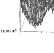
Figure 5: $\tau=90$

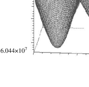
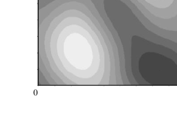
Figure 6: $\tau=450$

Figure 7: $\tau=720$

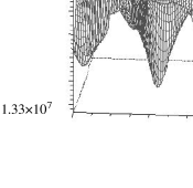
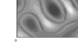
Figure 8: $\tau=1800$

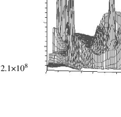
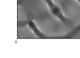
Figure 9: $\tau=2160$

Figure 10: $\tau=2430$

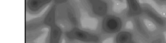
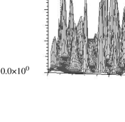
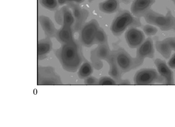
Figure 11: $\tau=2520$

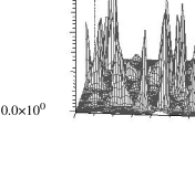
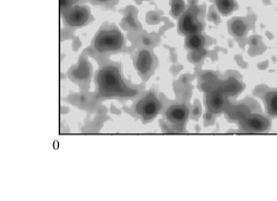
Figure 12: $\tau=2610$

Figure 13: $\tau=3060$

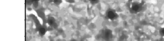
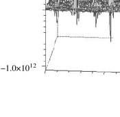
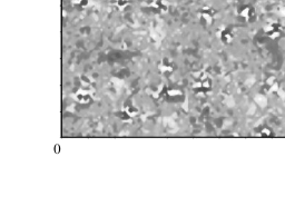
Figure 14: $\tau=3600$

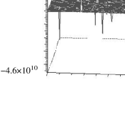
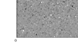
Figure 15: $\tau=5400$

Figure 16: $\tau=180000$

In Fig. 7 the initial small stochastic perturbations can be seen clearly. The fastest growing mode stars to dominate in Fig. 7, while the small perturbations are still visible. In Fig. 7 the growing modes are large enough for the initial perturbations to be no longer visible (they are obviously still present but due to the increasing scale they simply can no longer be seen). The linear growth continues in Fig. 10 until non-linear growth begins as depicted in Fig. 10. Rapid non-linear growth progresses and in Fig. 10 the fluctuations of the field are already $\sim{\cal O}(10^{4})$ while up to Fig. 10 they are only at the level $\sim{\cal O}(10^{-3})$. In Fig. 10 we can see how the lumps of charge are dynamically arranged in string-like features. These filaments are still visible in Fig. 13, where the condensate has further fragmented into lumps while the scale of the fluctuations has grown to $\sim{\cal O}(10^{11})$. The filament texture disappears from sight in the next two figures, Figs 13 and 13, while negative charge starts to develop (some traces of the filaments can still be seen in the distribution of charge lumps).

Up to this point the cases $x=1$ and $x\gg 1$ are qualitatively similar. If $x=1$, no negative charge develops and the lumps slowly relax into Q-balls while the universe expands which finally freezes the distribution. If, however, $x\gg 1$ like in the case shown here, new qualitative features become apparent after this point. Negatively charged lumps start to become visible in Fig. 16, and in Fig. 16 the ratio of positive to negative charge approaches one. The lumps of charge are complicated configurations that slowly relax into Q-balls and anti-Q-balls. Finally, in Fig. 16 we can see separate Q- and anti-Q-balls. The visible ten or so large Q-balls (anti-Q-balls) are only a very small fraction of the total number of Q-balls present in the lattice.

The different time scales of the fragmentation process can also be seen from Figs 7-16. The period of linear growth continues up to $\tau=2160$ after which rapid non-linear growth occurs between $\tau=2160-2520$. Negative lumps begin to form at around $\tau=3600$ while the relaxation process to Q-balls lasts until $\tau\sim 10^{5}$.

The process of Q-ball formation has been illustrated in more detail in Fig. 17. We are again considering a comoving volume and the scale of the figures is varied between different panels. The first panel is taken at $\tau=5400$ and the last panel at $\tau=180000$. Here $\omega=10^{-5}$ as before. In the first panel two large fluctuations that both carry large positive and negative charge densities are visible. Their shapes are still far from spherical and at this stage the future evolution of the fluctuations is far from obvious. In the following panels it can be seen that the initial complex configurations more or less develop into charge-anti charge -pairs that fluctuate and move with time. Eventually only one large ball remains from each of the two pairs. The final fate of the other partners cannot be determined from the Figures because of the presence of a large background. It may be annihilated in the process, or it may move away from the larger ball. It is clear, however, that the large balls are formed from these complex disturbances through a highly complicated relaxation process.

Figure 17: A detail of the Q-ball formation process

3.4 Distributions

The simulations allow us to determine the charge distribution of Q-balls and anti-Q-balls at different $\omega$ and time intervals. In practice we look for the distribution of the local charge maxima and minima since the charge of a ball is approximately proportional to these extremes. This is due to the fact that in the potential studied in this work, the Q-ball radius has only a weak dependence on the charge and the profile can be well approximated with a gaussian Ansatz [11]. The cumulative distributions are plotted in Fig. 18 for the cases $\omega=10^{0},\ \omega=10^{-5}$ with a detail of the $\omega=10^{-5}$-case enlarged.

Figure 18: Cumulative distributions for (a) $\omega=10^{-5}$, (b) $\omega=10^{0}$ and (c) a detail of the $\omega=10^{-5}$-case

As can be seen from the Fig. 18, the two cases are quite different from each other as expected. In the $\omega=10^{0}$ -case ($x\approx 1$) there form practically only positive balls, whereas in the $\omega=10^{-5}$ -case an approximately equal number of positive and negative balls are created. From the previous description of the Q-ball formation process, these differing features are expected. In the detail of the $\omega=10^{-5}$ -case one can also note that there is a small ’bump’ at zero charge density.

We can now compare the distributions obtained from simulations to the equilibrium distributions given in Sect. 2. The cumulative distribution function, $F(Q,\mu,\beta)$, for a thermal distribution in terms of the probability distribution function, $g(Q)=e^{\mu Q-\beta|Q|}(\beta|Q|+1)$, reads as (omitting the fugacity of the distribution)

$$\mbox{$$}F(Q,\mu,\beta)=\int\limits_{-\infty}^{Q}dQ^{\prime}g(Q^{\prime})=\int\limits_{-\infty}^{Q}dQ^{\prime}\epsilon^{\mu Q^{\prime}-\beta|Q^{\prime}|}(\beta|Q^{\prime}|+1).\vspace{\undereqskip}$$ (56)

However, as can be seen from Fig. 18, the distribution is not quite an equilibrium one but deviates slightly from the thermal one because of the presence of the ’bump’ at zero charge density. This feature is, however, a lattice artifact, as we will see.

Let us account for the ’bump’ by introducing a new probability density function

$$\mbox{$$}g(Q)=\left\{\begin{array}[]{ll}e^{\mu Q-\beta|Q|}(\beta|Q|+1),&|Q|\geq Q_{\min}\\ 0,&|Q|<Q_{\min},\end{array}\right.\vspace{\undereqskip}$$ (57)

where $Q_{\min}$ is a parameter to be determined by fitting to the numerical results. With this choice of the probability distribution function, the cumulative distribution function can be calculated to be

$$\mbox{$$}F(Q,\mu,\beta,Q_{\min})=y(\min\{Q,-Q_{\min}\})+y(Q_{\min})-y(\max\{Q,Q_{\min}\}),\vspace{\undereqskip}$$ (58)

where

$$\mbox{$$}y(Q)\equiv{Qe^{\mu Q-|Q|\beta}\over Q\beta-|Q|\mu}(1+|Q|\beta+{Q\beta\over Q\beta-|Q|\mu}).\vspace{\undereqskip}$$ (59)

We can now fit $y(Q)$ to the numerical data. An example is shown in Fig. 19 where $F(Q,\mu,\beta,Q_{\min})$ is fitted to the $\omega=10^{-5}$-cases at $\tau=180000$. $y(Q)$ fits the data generally quite well in all the cases where $x\gg 1$. If $\omega=10^{0}$ one obviously needs to consider a different type of fitting function since in this case no anti-Q-balls are present in the distribution.

Figure 19: A typical fit, $\omega=10^{-5}$

To test whether the inclusion of $Q_{\min}$ to the fitting parameters is justifiable we have also fitted $F(Q,\mu,\beta)$ to the data. In all the cases we found that this gives a much poorer fit. In Fig. 20 we have plotted $({a_{0}/a})^{2}\beta$ at different time intervals for the $\omega=10^{-5}$-case.

Figure 20: $m\beta$ at different time intervals

The $({a_{0}/a})^{2}$-factor is included to account for the expansion of the universe, since in two dimensions the total energy density of Q-balls in equilibrium behaves as $\sim 1/\beta$ for large $\beta$. On the other hand, the total energy is essentially conserved so that $a(t)^{2}/\beta(t)$ remains a constant of equilibrium.

From Fig. 20 it can be seen how $\beta$ quickly drops at around $\tau=3600-5400$. This corresponds to Figures 16 and 16. At this time the negative Q-balls start to form and the large initial charge lumps begin to fragment. The distribution then quickly thermalizes and is well described by the equilibrium distribution. We have run the simulation until $\tau=180000$ but in Fig. 20 we have only plotted a part of the whole simulated time interval. However, $({a_{0}/a})^{2}\beta$ stays constant until the end of the simulation.

The presence of the ’bump’ in the distribution may be attributed to a number of factors. To study whether it is a lattice induced effect we ran a number of simulations where the number of lattice points was different while keeping the physical sized of the fiducial volume constant. After the fitting procedure we found that $Q_{\min}$ decreases with the number of lattice points used. Therefore it is likely that the deviation from the simple thermal spectrum is just due to lattice effects. This conclusion is further supported by the fact that in the gravity mediated case the charge-energy relation is approximately linear, $E\sim Q$, so that there is no preference for the formation of large Q-balls over small Q-balls. In addition, when one considers the fact that the lattice spacing increases with time and that smaller balls have smaller radii it is not too surprising to see a small deviation from a purely thermal distribution at small charge density.

4 Conclusions

We have studied the process of Q-ball formation from the AD-condensate in the early universe by numerical simulations in two spatial dimensions. The analytical considerations presented in Sect. 2 reveal that a typical Q-ball is relativistic. This conclusion holds if at least part of the baryon asymmetry of the universe is contained in baryon number carrying Q-balls. The reaction rate of Q-ball interactions is then much larger than the Hubble rate and hence we may expect that a state of maximum entropy is likely to be reached. Assuming a thermal Q-ball distribution we showed that in a typical cosmological situation the AD-condensate fragments into practically equal numbers of Q-balls and anti-Q-balls so that $N_{+}\approx N_{-}$. The amount of charge contained in these balls is much larger than the net charge, $Q_{+}\approx Q_{-}\gg Q_{{tot}}$. Estimation of the average velocity of a Q-ball confirms that Q-balls are typically relativistic. The analytical calculations were carried out in both two and three dimensions and we found that the shapes of the number density distributions or velocities are only very weakly dependent on dimension. These considerations strongly support the assumption that 2-d simulations can in fact capture the essential features of the real 3-d case.

Our numerical simulations were carried out on a $2+1$ dimensional $100\times 100$-lattice. The initial condition was chosen to be uniform AD-condensate with small perturbations. The initial energy-to-charge ratio $x$ was varied from $1$ to $\sim 10^{5}$. We found that regardless of $x$ the qualitative behavior of the AD-condensate is similar in the beginning of the simulation. The small perturbations start to grow and due a complex dynamical process the AD-condensate fragments into several lumps carrying positive charge. These are not yet Q-balls but some excited states [14].

From this point on the further evolution of the condensate depends on the actual value of $x$. If $x=1$, the lumps slowly relax into Q-balls and no anti-Q-balls are present. This is what we would expect from analytical studies and this is what has been seen in 3-d lattice simulations [19, 20]. If, however, $x\gg 1$, the condensate fragments into a large number of Q- and anti-Q-balls, as we have shown here. We also showed that the distributions of the Q- and anti-Q-balls obtained from the simulations are thermal, which again is in accordance with analytical expectations.

An interesting feature which is apparent in Figs. 13-13 is that the system of AD lumps appears to possess some non-trivial spatial structure. First, the large Q- and anti-Q-balls can be seen to form in pairs which give rise to a positive spatial correlation between them. It should be noted that if small balls are also formed in pairs they are likely to have a homogenized spatial distribution due to their large velocities. Second, there are long range correlations which show up as filament-like structures in Figs. 10-13. The texture visible in the middle phase of the non-linear evolution may well survive in the spatial Q-ball distribution also at later times, although it no longer is visible. Numerical correlation analysis indeed shows that still at the final stage of our simulation (Fig. 13) the mean distance between both Q- and anti-Q-balls deviates by over four standard deviations from the random uniform distribution. The deviation is negative i.e. the mean distance between Q-balls is smaller than expected for a random distribution. These features may affect observables such as the cosmic microwave background or large scale structure and deserve further study.

The fact that the Q-ball distribution in the cosmologically realistic case, $x\gg 1$, tends toward a thermal one implies, like the analytical treatment shows, that a large number of Q-balls move relativistically. The very large Q-balls that are clearly visible in Fig. 16 appear immobile but there is also a large number of smaller fast moving Q-balls which can thermalize the distribution. In a thermodynamical sense one can view the fragmentation of the AD-condensate into Q-balls as a relaxation process where entropy is maximized: from this point of view the appearance of the thermal distribution is natural.

In this work we left the gauge mediated SUSY breaking scenario without the attention it deserves. This is due to a number of facts that make the simulation of the gauge mediated SUSY breaking scenario more cumbersome compared to the gravity mediated case. In the fragmentation process the spectra of growing modes play an important role since the first mode that goes non-linear determines the size of the fastest growing disturbance in the condensate. The SUSY breaking mechanism, i.e. whether it is gauge or gravity mediated, determines the size of the fastest growing mode via the actual form of the scalar potential. As we have seen, the size of the instabilities in the gauge mediated case are larger than in the gravity mediated scenario. Therefore one needs a lattice with a much larger physical size. Obviously, one can always increase lattice spacing but this happens at the cost of losing resolution. Moreover, the large instabilities correspond to large Q-balls forming from the AD-condensate which in the gauge mediated scenario have thin walls. To avoid numerical instabilities due to the thin walls a high resolution is required. Therefore, in order to avoid finite size effects, one would need a much larger number of lattice points than in the gravity mediated case.

In addition to the numerical difficulties the gauge mediated scenario does not benefit form the analytical arguments presented in Sect. 2. This is due to the different energy-charge -relations of the two cases. For large Q-balls in the gauge mediated case the energy is related to the charge by $E\sim Q^{3\over 4}$ instead of the linear relation $E\sim Q$ in the gravity mediated scenario. From (22) one can see that the Q-integral diverges since the $\exp(-\beta E+\mu Q)$-term is dominated by $\mu Q$ in the large Q limit in the gauge mediated scenario. Physically the lack of a proper asymptotic equilibrium state implies that the system tends towards a state where charge is concentrated in large balls (and ultimately in a single Q-ball) as noted also in Ref. [21]. However, one should also take into account that the more charge is stored in large balls the more there exists leftover energy in the system that must be accounted for. The final state of the system would then be strongly dependent on the time at which the distribution freezes due to the expansion of the universe and hence on the initial conditions.

To conclude, our results indicate that in the gravity mediated SUSY breaking case, the AD condensate fragments into an almost equal number of Q-balls and anti-Q-balls. The evaporation times of the Q-balls, the nature of particles they decay into, and possible spatial correlations surviving the fragmentation process and the subsequent decays of Q-balls, are obviously very important factors that determine the signatures left by a possible Q-ball period in the early history of the universe.

References

- [1]
- [2] M. Dine, L. Randall and S. Thomas, Nucl. Phys. B458 (1996) 291.
- [3] I. A. Affleck and M. Dine, Nucl. Phys. B249 (1985) 361.
- [4] S. Coleman, Nucl. Phys. B262 (1985) 263; A. Cohen, S. Coleman, H. Georgi and A. Manohar, Nucl. Phys. B272 (1986) 301.
- [5] A. Kusenko, Phys. Lett. B404 (1997) 285; Phys. Lett. B405 (1997) 108.
- [6] A. Kusenko and M. Shaposhnikov, Phys. Lett. B418 (1998) 46.
- [7] K. Enqvist and J. McDonald, Phys. Lett. B425 (1998) 309.
- [8] G. Dvali, A. Kusenko and M. Shaposhnikov, Phys. Lett. B417 (1998) 99.
- [9] S. Kasuya and M. Kawasaki, Phys Rev. Lett. 85 (2000) 2677.
- [10] A. Kusenko, V. Kuzmin, M. Shaposhnikov and P.G. Tinyakov, Phys Rev. Lett. 80 (1998) 3185; J. Arafune, T. Yoshida, S. Nakamura and K. Ogure, Phys. Rev. D62 (2000) 105013.
- [11] K.Enqvist and J.McDonald, Nucl. Phys. B538 (1999) 321.
- [12] K. Enqvist and J. McDonald, Phys. Lett. B440 (1998) 59; Phys Rev. Lett. 83 (1999) 2510.
- [13] K. Enqvist, A. Jokinen and J. McDonald, Phys. Lett. B483 (2000) 191.
- [14] K. Enqvist and J. McDonald, Nucl. Phys. B570 (2000) 407.
- [15] T. Multamäki and I. Vilja, Nucl. Phys. B574 (2000) 130.
- [16] M. Axenides et al., Phys. Rev. D61 (2000) 085006; R. Battye and P. Sutcliffe, hep-th/0003252.
- [17] T. Multamäki and I. Vilja, Phys. Lett. B482 (2000) 161.
- [18] T. Multamäki and I. Vilja, Phys. Lett. B484 (2000) 283.
- [19] S. Kasuya and M. Kawasaki, Phys. Rev. D 61 (2000) 041301.
- [20] S. Kasuya and M. Kawasaki, Phys. Rev. D 62 (2000) 023512.
- [21] M. Laine and M. Shaposhnikov, Nucl. Phys. B532 (1998) 376.