Report of the QCD Tools Working Group

Abstract

We report on the activities of the “QCD Tools for heavy flavors and new physics searches” working group of the Run II Workshop on QCD and Weak Bosons. The contributions cover the topics of improved parton showering and comparisons of Monte Carlo programs and resummation calculations, recent developments in PYTHIA, the methodology of measuring backgrounds to new physics searches, variable flavor number schemes for heavy quark electro-production, the underlying event in hard scattering processes, and the Monte Carlo MCFM for NLO processes.

1 Overview

The task of the “QCD Tools for heavy flavors and new physics searches working group” was to evaluate the status of the tools – invariably computer programs that simulate physics processes at colliders – that are being used to estimate signal and background rates at the Tevatron, and to isolate areas of concern. The contributions presented here cover several topics related to that endeavor. It is hoped that the next period of data-taking at the Tevatron will reveal indirect or direct evidence of physics beyond the Standard Model. The precise measurement of the $W$ boson mass $M_{W}$ and its correlation with the top quark mass $m_{t}$ is one example of an indirect probe of the Standard Model. The production of a light Higgs boson in association with a $W$ or $Z$ boson is an obvious example of a direct one. While both measurements are related to electroweak symmetry breaking, it requires a quantitative understanding of perturbative and non–perturbative QCD to interpret data.

Because of the importance of the $M_{W}$ measurement, and since gauge boson production in association with jets is a serious background in many new physics searches, much effort was devoted to understanding gauge boson production processes. It is well known that the emission of many soft gluons has a profound effect on the kinematics of gauge boson production. Two calculational methods have been used to compare “theory” with data: (1) analytic resummation of several series of important logarithms, and (2) parton showering based on DGLAP–evolved parton distribution functions. Here, there are reports on our understanding of both, and improvements. Note also that diboson production is often a background too.

In the Standard Model, and its minimal supersymmetric extension, the mechanism that generates mass for the electroweak gauge bosons also generates fermion mass. From an agnostic point of view, the fact that the $W$ and $Z$ bosons and the top quark have roughly similar masses, and these masses are quite disparate from, say, the electron or neutrino masses, is some evidence that heavy flavor is related to electroweak symmetry breaking. Many of the search strategies for Run II rely on tagging $c$ and $b$ quarks or $\tau$ leptons. For this reason, there are several contributions regarding issues of determining backgrounds in Run II.

2 Performing parton showering at Next-to-Leading-Order Accuracy

by S. Mrenna

2.1 Introduction

In the near future, experiments at the Tevatron will search for evidence of physics that supersedes the standard model. Important among the tools that will be used in these searches are showering event generators or showering Monte Carlos (SMC’s). Among the most versatile and popular of these are the Monte Carlos HERWIG[1], ISAJET[2], and PYTHIA[3]. SMC’s are useful because they accurately describe the emission of multiple soft gluons, which is, in effect, an all orders problem in QCD. However, they only predict total cross sections to a leading order accuracy, and, thus, can demonstrate a sizeable dependence on the choice of scale used for the parton distribution functions (PDF’s) or coupling constants (particularly $\alpha_{s}$). Also, in general, they do not translate smoothly into kinematic configurations where only one, hard parton is emitted. In distinction to SMC’s are certain analytic calculations which account for multiple soft gluon emission and higher order corrections to the hard scattering. These resummation calculations, however, integrate out the kinematics of the soft gluons, and, thus, are limited in their predictive power. They can, for example, describe the kinematics of a heavy gauge boson produced in hadron collision, but cannot predict the number or distribution of jets that accompany it. However, searches for new physics, either directly or indirectly through measurements of precision electroweak observables, often demand detailed knowledge of kinematic distributions and jet activity. Furthermore, $W$+jets (and $Z$+jets) processes are often backgrounds to SUSY or technicolor signatures, and we demand a reliable prediction of their properties. Here, we report on recent progress in improving the predictive power of showering Monte Carlos by incorporating the positive features of the analytic resummation calculations into the showering algorithms. In the ensuing discussion, we focus on the specific example of $W$ boson production at a hadron collider, when the $W$ decays leptonically. The results apply equally well to $\gamma^{*},Z$ and Higgs bosons (or any heavy, color–singlet particle) produced in hadron collisions.

2.2 Parton Showers

SMC’s are based on the factorization theorem [4], which, roughly, states that physical observables in QCD are the product of short–distance functions and long–distance functions. The short–distance functions are calculable in perturbation theory. The long–distance functions are fit at a scale, but their evolution to any other scale is also calculable in perturbation theory.

A standard application of the factorization theorem is to describe $W$ boson production at a $p\bar{p}$ collider at a fixed order in $\alpha_{s}$. The production cross section is obtained by convoluting the partonic subprocesses evaluated at the scale $Q$ with the PDF’s evaluated at $Q$. The partons involved in the hard collision must be sufficiently virtual to be resolved inside the proton, and a natural choice for the scale $Q$ is $Q=M_{W}$ [5]. However, the valence quarks in the proton have virtualities at a much lower scale $Q_{0}$ of the order of 1 GeV. The connection between the partons at the low scale $Q_{0}$ and those at the high scale $Q$ is described by the DGLAP evolution equations [6]. The DGLAP equations include the most important kinematic configurations of the splittings $a\to bc$, where $a,b$ and $c$ represent different types of partons in the hadron ($q,g$, etc.). Starting from a measurement of the PDF’s at a low scale $Q_{0}$, a solution of the DGLAP equations yields the PDF’s at the hard scale $Q$. Equivalently, starting with a parton $c$ involved in a hard collision, it is also possible to determine probabilistically which splittings generated $c$. In the process of evolving parton $c$ back to the valence quarks in the proton, a number of spectator partons (e.g. parton $b$ in the branching $a\to bc$) are resolved. These partons constitute a shower of soft and/or collinear jets that accompany the $W$–boson, and influence its kinematics.

The shower described above occurs with unit probability and does not change the total cross section for $W$–boson production calculated at the scale $Q$ [7]. The showering can be attached to the hard–scattering process based on a probability distribution after the hard scattering has been selected. Once kinematic cuts are applied, the transverse momentum and rapidity of the $W$–boson populate regions never accessed by the differential partonic cross section calculated at a fixed order. This is consistent, since the fixed–order calculation was inclusive (i.e., $p\bar{p}\to W+X$) and was never intended to describe the detailed kinematics of the $W$–boson in isolation. The parton shower, in effect, resolves the structure of the inclusive state of partons denoted as $X$. In practice, the fixed order partonic cross section (without showering) can still be used to describe properties of the decay leptons as long as the observable is well defined (e.g., the number of leptons with central rapidity and high transverse momentum, but not the distribution of transverse momentum of the $W$).

Here, we focus on the case of initial state gluon radiation. More details can be found in Ref. [8], for example. Showering of the parton $b$ with momentum fraction $x$ resolved at the scale $Q^{2}=e^{t}$ is driven by a Sudakov form factor $\exp(-S)$, such as[9]

$$\exp\!\!\left(-\!\!\int_{t^{\prime}}^{t}\!\int_{x\over 1-\epsilon}^{x\over x+\epsilon}dt^{\prime\prime}dz{\alpha_{s}(z,t^{\prime\prime})\over 2\pi}\hat{P}_{a\to bc}(z){x^{\prime}f_{a}(x^{\prime},t^{\prime})\over xf_{b}(x,t^{\prime})}\!\right),\\ x^{\prime}=x/z,$$ (1)

which is implemented in PYTHIA, and the formally equivalent expression[10]

$${\Delta(t^{\prime})\over f_{b}(x,t^{\prime})}{f_{a}(x,t)\over\Delta(t)},\\ \Delta(t^{\prime})=\exp\!\!\left(-\!\!\int_{t_{0}}^{t^{\prime}}\!\int_{\epsilon}^{1-\epsilon}dt^{\prime\prime}dz{\alpha_{s}(z,t^{\prime\prime})\over 2\pi}\hat{P}_{a\to bc}(z)\right),$$ (2)

which is implemented in HERWIG. In the above expressions, $t_{0}$ is a cutoff scale for the showering, $\hat{P}$ is a DGLAP splitting function, and $f_{i}$ is a parton distribution function. The Sudakov form factor presented here is a solution of the DGLAP equation, and gives the probability of evolving from the scale ${Q}^{2}=e^{t}$ to ${Q^{\prime}}^{2}=e^{t^{\prime}}$ with no resolvable branching. The Sudakov form factor contains all the information necessary to reconstruct a shower, since it encodes the change in virtuality of a parton until a resolvable showering occurs. A parton shower is then an iterative solution of the equation $r=\exp(-S)$, where $r$ is a random number uniformly distributed in the interval $[0,1]$, until a solution for $Q^{\prime}$ is found which is below a cutoff. For consistency, the cutoff should represent the lowest scale of resolvable emission $Q_{0}$. The evolution proceeds backwards from a large, negative scale $-|Q^{2}|$ to a small, negative cutoff scale $-|Q_{0}^{2}|$.

After choosing the change in virtuality, a particular backwards branching and the splitting variable $z$ are selected from the probability function based on their relative weights (a summation over all possible branchings $a\to bc$ is implied in these expressions). The details of how a full shower is reconstructed in the PYTHIA Monte Carlo, for example, can be found in Ref. [3]. The structure of the shower can be complex: the transverse momentum of the $W$–boson is built up from a whole series of splittings and boosts, and is known only at the end of the shower, after the final boost.

The SMC formulation outlined above is fairly independent of the hard scattering process considered. Only the initial choice of partons and possibly the high scale differs. Therefore, this formalism can be applied universally to many different scattering problems. In effect, soft and collinear gluons are not sensitive to the specifics of the hard scattering, only the color charge of the incoming partons.

2.3 Analytic Resummation

At hadron colliders, the partonic cross sections can receive substantial corrections at higher orders in $\alpha_{s}$. This affects not only the total production rate, but also the kinematics of the $W$ boson. At leading order ($\alpha_{s}^{0}$), the $W$–boson has a $\delta(Q_{T}^{2})$ distribution in $Q_{T}^{2}$. At next–to–leading order, the real emission of a single gluon generates a contribution to $d\sigma/dQ_{T}^{2}$ that behaves as $Q_{T}^{-2}\alpha_{s}(Q_{T}^{2})$ and $Q_{T}^{-2}\alpha_{s}(Q_{T}^{2})\ln(Q^{2}/Q_{T}^{2})$ while the leading order, soft, and virtual corrections are proportional to $-\delta(Q_{T}^{2})$. At higher orders, the most singular terms follow the pattern of $\alpha_{s}(Q_{T}^{2})^{n}\sum_{m=0}^{2n-1}\ln^{m}(Q^{2}/Q_{T}^{2})$ $=\alpha_{s}^{n}L^{m}\equiv V^{n}$. The logarithms arise from the incomplete cancellation of the virtual and real QCD corrections, but this cancellation becomes complete for the integrated spectrum, where the real gluon can become arbitrarily soft and/or collinear to other partons. The pattern of singular terms suggest that perturbation theory should be performed in powers of $V^{n}$ instead of $\alpha_{s}^{n}$. This reorganization of the perturbative series is called resummation.

The first studies of soft gluon emission resummed the leading logarithms [11, 12], leading to a suppression of the cross section at small $Q_{T}$. The suppression underlies the importance of including sub–leading logarithms [13]. The most rigorous approach to the problem of multiple gluon emission is the Collins–Soper–Sterman (CSS) formalism for transverse momentum resummation [14], which resums all of the important logarithms. This is achieved after a Fourier transformation with respect to $Q_{T}$ in the variable $b$, so that the series involving the delta function and terms $V^{n}$ simplifies to the form of an exponential. Hence, the soft gluon emission is resummed or exponentiated in this $b$–space formalism. Despite the successes of the $b$–space formalism, there are drawbacks: the soft gluon dynamics are integrated out, and the Sudakov form factor is a Fourier transform.

The CSS formalism was used by its authors to predict both the total cross section to NLO and the kinematic distributions of the $W$–boson to all orders [15] at hadron colliders. A similar treatment was presented using the AEGM formalism [16], that does not involve a Fourier transform, but is evaluated directly in transverse momentum $Q_{T}$ space. When evaluated at NLO, the two formalisms are equivalent to NNNL order in $\alpha_{s}$, and agree with the fixed order calculation of the total cross section [17]. A more detailed numerical comparison of the two predictions can be found in Ref. [18].

Recently, the AEGM formalism has been re-investigated, and an approximation to the $b$–space formalism has been developed in $Q_{T}$–space which retains its predictive features [19] (see also the recent eprint [20]). This formulation does have a simple, physical interpretation, and can be used to develop an alternate algorithm for parton showering which includes higher–order corrections to the hard scattering. For this reason, we focus on the $Q_{T}$–space formalism. To NNNL accuracy, the $Q_{T}$ space expression agrees exactly with the $b$–space expression, and has the form [19]:

$$\begin{split}{d\sigma(h_{1}h_{2}\to V^{(*)}X)\over dQ^{2}\,dQ^{2}_{T}\,dy}={d\over dQ_{T}^{2}}\widetilde{W}(Q_{T},Q,x_{1},x_{2})\\ +Y(Q_{T},Q,x_{1},x_{2}).\end{split}$$ (3)

In this expression, $Q$, $Q_{T}$ and $y$ describe the kinematics of the boson $V$, the function $Y$ is regular as $Q_{T}\to 0$ and corrects for the soft gluon approximation, and the function $\widetilde{W}$ has the form:

$$\begin{split}{\widetilde{W}}=&e^{-S(Q_{T},Q)}H(Q,y)\times\\ &\Big{(}C\otimes f\Big{)}(x_{1},Q_{T})\Big{(}C\otimes f\Big{)}(x_{2},Q_{T}),\end{split}$$ (4)

where

$$\begin{split}S(Q_{T},Q)=&\\ \int_{Q_{T}^{2}}^{Q^{2}}{d{\bar{\mu}}^{2}\over{\bar{\mu}}^{2}}&\left[\ln{Q^{2}\over{\bar{\mu}}^{2}}A\big{(}\alpha_{s}({\bar{\mu}})\big{)}+B\big{(}\alpha_{s}({\bar{\mu}})\big{)}\right],\end{split}$$ (5)

and

$$\left(C_{jl}\otimes f_{l/h_{1}}\right)(x_{1},\mu)=\\[2.84526pt] \int_{x_{1}}^{1}{d\xi_{1}\over\xi_{1}}\,C_{jl}({x_{1}\over\xi_{1}},Q_{T})f_{l/h_{1}}(\xi_{1},Q_{T}).$$ (6)

$H$ is a function that describes the hard scattering, and $A$, $B$, and $C$ are calculated perturbatively in powers of $\alpha_{s}$:

$$(A,B,C)=\sum_{n=0}^{\infty}\left({\alpha_{s}(\mu)\over\pi}\right)^{n}(A,B,C)^{(n)}$$

(the first non–zero terms in the expansion of $A$ and $B$ are for $n=1$). The functions $C^{(n)}$ are the Wilson coefficients, and are responsible for the change in the total production cross section at higher orders. In fact, $\left(C\otimes f\right)$ is simply a redefinition of the parton distribution function obtained by convoluting the standard ones with an ultraviolet–safe function.

Ignoring $Y$ and other kinematical dependence, Eq. (3) can be rewritten as:

$${d\sigma(h_{1}h_{2}\to WX)\over dQ_{T}^{2}}=\sigma_{1}\left({d\over dQ_{T}^{2}}\left[e^{-S(Q_{T},Q)}~{}R\right]\right),$$ (7)

where

$$R={\left(C\otimes f\right)(x_{1},Q_{T})\left(C\otimes f\right)(x_{2},Q_{T})\over\left(C\otimes f\right)(x_{1},Q)\left(C\otimes f\right)(x_{2},Q)}$$ (8)

and

$$\sigma_{1}=\kappa\int{dx_{1}\over x_{1}}\left(C\otimes f\right)(x_{1},Q)\left(C\otimes f\right)(x_{2},Q).$$

The factor $\sigma_{1}$ is the total cross section to a fixed order, while the rest of the function yields the probability that the $W$–boson has a transverse momentum $Q_{T}$.

At leading order, the expression for the production of an on–shell $W$–boson simplifies considerably to:

$${d\sigma(h_{1}h_{2}\to WX)\over dQ^{2}_{T}}=\\[2.84526pt] \sigma_{0}{d\over dQ^{2}_{T}}\left(e^{-S(Q_{T},Q)}{f(x_{1},Q_{T})f(x_{2},Q_{T})\over f(x_{1},Q)f(x_{2},Q)}\right),$$ (9)

$$\sigma_{0}=\kappa\int{dx_{1}\over x_{1}}f(x_{1},Q)f(x_{2},Q),$$

where $\kappa$ contains physical constants and we ignore the function $Y$ for now. The expression contains two factors, the total cross section at leading order $\sigma_{0}$, and a cumulative probability function in $Q_{T}^{2}$ that describes the transverse momentum of the $W$–boson. The term $e^{-S/2}f(x,Q_{T})/f(x,Q)$ is of the same form as the Sudakov form factor of Eq. (2) and, hence, to that of Eq. (1).

2.4 A modified showering algorithm

The primary result of this analysis is to exploit the expression for the differential cross section, which has the form of a leading order cross section times a backwards evolution, to incorporate NLO corrections to the parton shower. We generalize the function $\Delta(t)/f(x,t)\times f(x,t^{\prime})/\Delta(t^{\prime})$ of the standard backwards showering algorithm to $\sqrt{\widetilde{W}}$ (the square root appears because we are considering the evolution of each parton line individually).

To implement this modification in a numerical program, like PYTHIA, we need to provide the new, modified PDF (mPDF) based on the Wilson coefficients. At leading order, the only Wilson coefficient is $C_{ij}^{(0)}=\delta_{ij}\delta(1-z)$, and we reproduce exactly the standard showering formulation. For $W$–boson production at NLO, the Wilson coefficients $C$ are:

$$C_{jk}^{(1)} = \delta_{jk}\left\{{2\over 3}(1-z)+{1\over 3}(\pi^{2}-8)\delta(1-z)\right\},$$ (10)

$$C_{jg}^{(1)} = {1\over 2}z(1-z).$$ (11)

To NLO, the convolution integrals become:

$$\left(C\otimes f_{i}\right)(x,\mu)=f_{i}(x,\mu)\left(1+{\alpha_{s}(\mu)\over\pi}{1\over 3}(\pi^{2}-8)\right)\\[2.84526pt] +{\alpha_{s}(\mu)\over\pi}\int_{x}^{1}{dz\over z}\left[{2\over 3}(1-z)f_{i}(x/z,\mu)\right.\\[2.84526pt] \left.+{1\over 2}(1-z)f_{g}(x/z,\mu)\right],$$ (12)

and $f_{g}(x,\mu)$ is unchanged. The first term gives the contribution of an unevolved parton to the hard scattering, while the other two contain contributions from quarks and gluons with higher momentum fractions that split $q\to qg$ and $g\to q\bar{q}$, respectively.

We are assuming that the Sudakov form factor used in the analytic expressions and in the SMC are equivalent. In fact, the integration over the quark splitting function in $\Delta(Q)$ yields an expression similar to the analytic Sudakov:

$$\int_{z_{m}}^{1-z_{m}}dzC_{F}\left({1+z^{2}\over 1-z}\right)=\\[2.84526pt] C_{F}\left(\ln\left[{1-z_{m}\over z_{m}}\right]^{2}-3/2(1-2z_{m})\right)\\[2.84526pt] \simeq A^{(1)}\ln(Q^{2}/Q_{T}^{2})+B^{(1)},$$ (13)

where $z_{m}={Q_{T}\over(Q+Q_{T})}$ is an infrared cutoff, terms of order $z_{m}$ and higher are neglected, and the $z$ dependence of the running coupling has been ignored [21]. Note that the coefficients $A^{(1)}$ ($C_{F}$) and $B^{(1)}$ ($-3/2C_{F}$) are universal to $q\bar{q}$ annihilation into a color singlet object, just as the showering Sudakov form factor only knows about the partons and not the details of the hard scattering. For $gg$ fusion, only the coefficient $A^{(1)}$ (3) is universal. In general, at higher orders, the analytic Sudakov is sensitive to the exact hard scattering process.

While the Sudakov form factors are similar, there is no one–to–one correspondence. First, the $Q_{T}$–space Sudakov form factor is expressed directly in terms of the $Q_{T}$ of the heavy boson, while, in the SMC’s, the final $Q_{T}$ is built up from a series of branchings. Secondly, the integral on the left of Eq. (13) is positive (provided that $z_{m}<\frac{1}{2}$), while the analytic expression on the right can become negative. This is disturbing, since it means sub-leading logarithms (proportional to $B$) are dominating leading ones. In the exact SMC Sudakov, the kinematic constraints guarantee that $\Delta(Q)<1$. In this sense, the Sudakov in the SMC is a more exact implementation of the analytic one. Nonetheless, the agreement apparent between the analytic and parton shower expressions is compelling enough to proceed assuming the two Sudakov form factors are equivalent.

2.5 Hard Emission Corrections

The SMC and resummation formalisms are optimized to deal with kinematic configurations that have logarithmic enhancements $L$. For large $Q_{T}\simeq Q$, there are no such enhancements, and a fixed order calculation yields the most accurate predictions. The region of medium $Q_{T}$, however, is not suited to either particular expansion, in $\alpha_{s}^{n}L^{m}$ or $\alpha_{s}^{n}$.

The problem becomes acute for SMC’s. In the standard implementation of SMC’s, the highest $Q_{T}$ is set by the maximum virtuality allowed, $Q=M_{W}$ in our example, so that the region $Q_{T}\geq Q$ is never accessed. However, at $Q_{T}\geq Q$, the fixed order calculation is preferred and yields a non–zero result, so there is a discontinuity between the two predictions. This behavior does not occur in the analytic resummation calculations, because contributions to the cross section that are not logarithmically enhanced as $Q_{T}\to 0$ are added back order–by–order in $\alpha_{s}$. This procedure corrects for the approximations made in deriving the exponentiation of soft gluon emission. The correction is denoted $Y$. If the coefficients $A$ and $B$ are calculated to high–enough accuracy, one sees a relatively smooth transition between Eq. (3) and the NLO prediction at $Q_{T}=Q$. In the $Q_{T}$–space calculation, this matching between the two calculations at $Q_{T}=Q$ is guaranteed at any order. The function $Y$ has the form

$$Y(Q_{T},Q,x_{1},x_{2})=\int_{x_{1}}^{1}{\frac{d\xi_{1}}{\xi_{1}}}\int_{x_{2}}^{1}{\frac{d\xi_{2}}{\xi_{2}}}\sum_{n=1}^{\infty}\left[{\frac{\alpha_{s}(Q)}{\pi}}\right]^{n}\\[2.84526pt] f_{a}(\xi_{1},Q)\,R_{ab}^{(n)}(Q_{T},Q,\frac{x_{1}}{\xi_{1}},\frac{x_{2}}{\xi_{2}})\,f_{b}(\xi_{2},Q).$$ (14)

For $W$ or $Z$ boson production, the $a=q,b=\bar{q}$ component of $R$ at first order in $\alpha_{s}$ is

$$R^{(1)}_{q\bar{q}}=C_{F}{{(\hat{t}-Q^{2})^{2}+(\hat{u}-Q^{2})^{2}}\over{\hat{t}\hat{u}}}\delta(\hat{s}+\hat{t}+\hat{u}-Q^{2})\\[2.84526pt] -{1\over Q_{T}^{2}}\hat{P}_{q\to q}(z_{B})\delta(1-z_{A})-(A\leftrightarrow B).$$ (15)

The invariants $\hat{s},\hat{t}$ and $\hat{u}$ are defined in terms of $z,Q,Q_{T}$:

$$\begin{split}&\hat{t}/Q^{2}=1-1/z_{B}\sqrt{1+Q_{T}^{2}/Q^{2}},\\ &\hat{u}/Q^{2}=1-1/z_{A}\sqrt{1+Q_{T}^{2}/Q^{2}}.\end{split}$$ (16)

The term in $R$ proportional to the delta function is simply the squared matrix element for the hard emission, while the terms proportional to $Q_{T}^{-2}$ are the asymptotic pieces from $\widetilde{W}$.

We would like to include similar corrections into the SMC. However, this is not entirely straightforward. Though it is not obvious from Eq. (14), the ($a=g,b=q$+permutations) components are negative for $Q_{T}<Q$, though the sum $Y$ is positive. Retaining negative weights in an intermediate part of the calculation is not a problem in principle. We can artificially force the negative weights to be positive, and then include the correct sign of the weight when filling histograms, for example. However, this would involve some modification to the PYTHIA code used in this study.

A pragmatic approach is to ignore the negative weights entirely, and multiply the exact $W+$parton cross sections by a factor so that their sum reproduces the $Q_{T}$ distribution and normalization of the analytic $Y$ piece. For the Tevatron in Run I, we find that the multiplicative factor $f_{\rm COR}={1\over 2}(Q_{T}/50)^{2}\times(1+Q_{T}/25)$ reproduces the correct behavior for $Q_{T}<50$ GeV. For $Q_{T}\geq 50$ GeV, the uncorrected $W+$ parton cross sections are employed. Since the matching between the “resummed” and “fixed order” calculations is now occurring at $Q_{T}=50$ GeV instead of $Q_{T}=M_{W}$, we further limit the maximum virtuality of showering to $50$ GeV. This is in accord with the fact that the “resummed” part of the analytic calculation becomes negative around $Q_{T}=50$ GeV. This choice does have some effect on the overall normalization of the parton showering component.

At this point, it is useful to compare the scheme outlined above to other approaches at improving the showering algorithm. One scheme is based on phase–space splitting of a NLO matrix element into a piece with LO kinematics and another with exclusive NLO kinematics [23, 24]. The separation depends on an adjustable parameter that splits the phase space. In the approach of Ref. [23], the separation parameter is tuned so that the contribution with LO kinematics vanishes. The resultant showering of the term with exclusive NLO kinematics can generate emissions which are harder than the first “hard” emission, which is not consistent. More seriously, physical observables are sensitive to the exact choice of the separation parameter (see the discussion in Ref. [22] regarding $Q_{T}^{sep}$). Furthermore, the separation parameter must be retuned for different processes and different colliders. This scheme is guaranteed to give the NLO cross section before cuts, but does not necessarily generate the correct kinematics.

The other scheme is to modify the showering to reproduce the hard emission limit [25, 26]. While this can be accomplished, it does so at the expense of transferring events from low $Q_{T}$ to high $Q_{T}$. There is no attempt to predict the absolute event rate, but only to generate the correct event shapes. In some implementations, the high scale of the showering is increased to the maximum virtuality allowed by the collider energy. This is contrary to the analytic calculations, where the scale $Q=M_{W}$, for example, appears naturally (in the choice of constants $C_{1},C_{2}$ and $C_{3}$ which eliminate potentially large logarithms). This scheme will generate the correct hard limit, but will not generate the correct cross section in the soft limit.

2.6 Numerical results

For our numerical results, we predict the $Q_{T}$ distribution of $W$ and $Z$ bosons produced at the Tevatron in Run I. The modified PDF (mPDF) was calculated using CTEQ4M PDF’s. These distributions are in good agreement with analytic calculations, but the shape and overall normalization cannot be predicted accurately by the standard showering algorithm. Some of the alternative showering algorithms reproduce the shape, but not the overall normalization. Secondly, we discuss jet properties for the same processes, which are not significantly altered from the predictions of the standard showering algorithm. These cannot be predicted by analytic calculations.

Figure 1: $(a)$ The prediction of the $W$ boson transverse momentum distribution in Run I at the Tevatron (solid line) compared to the DØ data. The prediction includes the effects of the modified parton distribution functions, the correction to the hard scattering process, and a primordial $k_{T}$ of 2.0 GeV; (b) The prediction of the $Z$ boson transverse momentum distribution in Run I at the Tevatron (solid line) compared to the CDF data. The prediction includes the effects of the modified parton distribution functions, the correction to the hard scattering process, and a primordial $k_{T}$ of 2.0 GeV.

In Fig. 1(a), the transverse momentum of the $W$ boson (solid line) as predicted by the algorithm outlined above is shown in comparison to DØ data[27] (crosses). The theoretical distribution has been passed through the CMS detector simulation. As in analytic calculations, the position of the peak in the $Q_{T}$ distribution from parton showering depends on non–perturbative physics [29]. In PYTHIA, this is implemented through a Gaussian smearing of the transverse momentum of the incoming partons. To generate this plot, we have changed the default Gaussian width from .44 GeV to 2.0 GeV, which is more in accord with other analyses. This is the value used in all subsequent results. Because of the necessity of reconstructing the missing $E_{T}$ in $W$ boson decays to leptons, the smearing of the $Q_{T}$ distribution is significant, and the agreement between the prediction and data is not a rigorous test of the modified showering algorithm. Fig. 1(b) shows the comparison of the CDF Drell–Yan data [28] near the $Z^{0}$ peak to the modified showering prediction. While there is a problem with the overall normalization, the shape agreement is very good. We note that there is also a problem with the overall normalization of the analytic resummation predictions.

Given all the effort necessary to improve the showering, it is reasonable to ask if the similar results would have been obtained by simply renormalizing the usual predictions to the NLO rate, i.e. using PYTHIA but applying a constant $K$–factor at the end. In $W$ boson production, the relative size of the $Q_{T}$ distributions vary by as much as 10% in the important regions of small and medium $Q_{T}$. Of course, the effect is much larger for the large $Q_{T}$ region where there is almost no rate from the standard parton showering. If one is worried about precision measurements or is applying kinematic cuts that bias the large $Q_{T}$ region, then standard parton showering can yield misleading results. In most cases, however, it appears to be perfectly reasonable to renormalize the parton showering results to the total NLO cross section. We have also checked if our new showering algorithm has an impact on jet properties. For $W$ and $Z$ boson production, there are only minor differences, which is expected since the Wilson coefficients for $W$ and $Z$ boson production are nearly unity. In general, we do not expect any major changes from using the modified PDF’s, since the showering depends on the ratio of the modified PDF’s evaluated at two different scales, which is not as sensitive to the overall normalization of the PDF.

2.7 Conclusions

We have presented a modified, parton showering algorithm that produces the total cross section and the event shapes beyond the leading order. These modifications are based on the $Q_{T}$–space resummation. The parton showering itself is modified by using a new PDF (called mPDF) which encodes some information about the hard scattering process. Simultaneously, the explicit, hard emission is included, but only after subtracting out the contribution already generated by the showering: this correction is called $Y$. The presence of $Y$ yields a smooth transition from the parton showering to single, hard emission. We modified the PYTHIA Monte Carlo to account for these corrections, and presented comparisons with Run I $W$ and $Z$ boson data.

The scheme works well for the cases considered in this study, and the correct cross sections, transverse momentum distributions, and jet properties are generated. We have compared our kinematic distributions to the case when the results of the standard showering are multiplied by a constant $K$–factor to reproduce the NLO cross section. We find variations on the order of 10% for small and medium transverse momentum.

There are several effects which still need study. We have not included the exact distributions for the decay of the leptons [30] for $W$ and $Z$ production, which are resummed differently. It is straightforward to include such effects. In the theoretical discussion and numerical results, we have focussed on initial state radiation, but our results should apply equally well for final state radiation. The situation is certainly simpler, since final state radiation does not require detailed knowledge of the fragmentation functions. Also, the case when color flows from the initial state to the final state requires study. A resummed calculation already exists for the case of deep inelastic scattering [31], and much theoretical progress has been made for heavy quark production [32]. We believe that the modified showering scheme outlined in this study generalizes beyond NLO, just as the analytic calculations can be calculated to any given order. For example, we could include hard $W+2$ jet corrections [33] to $Y$. For consistency, however, higher order terms ($A$ and $B$) may also need to be included in the Sudakov form factor.

The modified PYTHIA subroutines used in this study and an explanation of how to use them are available at the following URL:
moose.ucdavis.edu/mrenna/shower.html.

Acknowledgements I thank C–P Yuan and T. Sjöstrand for many useful discussions and encouragement in completing this work. This work was supported by United States Department of Energy and the Davis Institute for High Energy Physics.

3 Recent Progress in PYTHIA

by T. Sjöstrand

3.1 Introduction

A general-purpose generator in high-energy physics should address a number of physics aspects, such as:

• the matrix elements for a multitude of hard subprocesses of interest,

• the convolution with parton distributions to obtain the hard-scattering kinematics and cross sections,

• resonance decays that (more or less) form part of the hard subprocess (such as $W$, $Z$, $t$ or $h$),

• initial- and final-state QCD and QED showers (or, as an alternative, higher-order matrix elements, including a consistent treatment of virtual-correction terms),

• multiple parton–parton interactions,

• beam remnants,

• hadronization,

• decay chains of unstable particles, and

• general utility and analysis routines (such as jet finding).

However, even if a Monte Carlo includes all the physics we currently know of, there is no guarantee that not some important aspect of the physics is missing. Certain assumptions and phenomenological models inside the program are not well tested and will not necessarily hold when extrapolated to different energy regimes. For example, the strong-interaction dynamics in QCD remains unsolved and thereby unpredictable in an absolute sense.

The PYTHIA 6.1 program was released in March 1997, as a merger of JETSET 7.4, PYTHIA 5.7 [3] and SPYTHIA [34]. It addresses all of the aspects listed above. The current subversion is PYTHIA 6.136, which contains over 50,000 lines of Fortran 77 code. The code, manuals and sample main programs may be found at
http://www.thep.lu.se/$\sim$torbjorn/Pythia.html .

The two other programs of a similar scope are HERWIG[1] and ISAJET[2] . For parton-level processes, many more programs have been written. The availability of several generators provides for useful cross-checks and a healthy competition. Since the physics of a complete hadronic event is very complex and only partially understood from first principles, one should not prematurely converge on one single approach.

3.2 PYTHIA 6.1 Main News

Relative to previous versions, the main news in PYTHIA 6.1 includes

• a renaming of the old JETSET program elements to begin with PY, therefore now standard throughout,

• new SUSY processes and improved SUSY simulation relative to SPYTHIA, and new PDG codes for sparticles,

• new processes for Higgs (including doubly-charged in left–right symmetric models), technicolor, …,

• several improved resonance decays, including an alternative Higgs mass shape,

• some newer parton distributions, such as CTEQ5 [35],

• initial-state showers matched to some matrix elements,

• new options for final-state gluon splitting to a pair of $c/b$ quarks and modified modeling of initial-state flavor excitation,

• an energy-dependent $p_{\perp\mathrm{min}}$ in multiple interactions,

• an improved modeling of the hadronization of small-mass strings, of importance especially for $c/b$, and

• a built-in package for one-dimensional histograms (based on GBOOK).

Some of these topics will be further studied below. Other improvements, of less relevance for $\overline{p}p$ colliders, include

• improved modeling of gluon emission off $c/b$ quarks in $e^{+}e^{-}$,

• color rearrangement options for $W^{+}W^{-}$ events,

• a Bose-Einstein algorithm expanded with new options,

• a new alternative baryon production scheme [36],

• QED radiation off an incoming muon,

• a new machinery to handle real and virtual photon fluxes, cross sections and parton distributions [37], and

• new standard interfaces for the matching to external generators of two, four and six fermions (and of two quarks plus two gluons) in $e^{+}e^{-}$.

The current list of over 200 different subprocesses covers topics such as hard and soft QCD, heavy flavors, DIS and $\gamma\gamma$, electroweak production of $\gamma^{*}/Z^{0}$ and $W^{\pm}$ (singly or in pairs), production of a light or a heavy Standard Model Higgs, or of various Higgs states in supersymmetric (SUSY) or left–right symmetric models, SUSY particle production (sfermions, gauginos, etc.), technicolor, new gauge bosons, compositeness, and leptoquarks.

Needless to say, most users will still find that their particular area of interest is not as well addressed as could be wished. In some areas, progress will require new ideas, while lack of time and manpower is the limiting factor in others.

3.3 Matching To Matrix Elements

The matrix-element (ME) and parton-shower (PS) approaches to higher-order QCD corrections both have their advantages and disadvantages. The former offers a systematic expansion in orders of $\alpha_{s}$, and a powerful machinery to handle multiparton configurations on the Born level, but loop calculations are tough and lead to messy cancellations at small resolution scales. Resummed matrix elements may circumvent the latter problem for specific quantities, but then do not provide exclusive accompanying events. Parton showers are based on an improved leading-log (almost next-to-leading-log) approximation, and so cannot be accurate for well separated partons, but they offer a simple, process-independent machinery that gives a smooth blending of event classes (by Sudakov form factors) and a natural match to hadronization. It is therefore natural to try to combine these descriptions, so that ME results are recovered for widely separated partons while the PS sets the subjet structure.

For final-state showers in $Z^{0}\to q\overline{q}$, corrections to the showering were considered quite a while ago [38], e.g. by letting the shower slightly overpopulate the $q\overline{q}g$ phase space and then using a Monte Carlo veto technique to reduce down to the ME level. This approach easily carries over to showers in other color-singlet resonance decays, although the various relevant ME’s have not all been implemented in PYTHIA so far.

A similar technique is now available for the description of initial-state radiation in the production of a single color-singlet resonance, such as $\gamma^{*}/Z^{0}/W^{\pm}$ [39]. The basic idea is to map the kinematics between the PS and ME descriptions, and to find a correction factor that can be applied to hard emissions in the shower so as to bring agreement with the matrix-element expression. Some simple algebra shows that, with the PYTHIA shower kinematics definitions, the two $q\overline{q}^{\prime}\to gW^{\pm}$ emission rates disagree by a factor

$$R_{q\overline{q}^{\prime}\to gW}(\hat{s},\hat{t})=\frac{(\mathrm{d}\hat{\sigma}/\mathrm{d}\hat{t})_{\mathrm{ME}}}{(\mathrm{d}\hat{\sigma}/\mathrm{d}\hat{t})_{\mathrm{PS}}}=\frac{\hat{t}^{2}+\hat{u}^{2}+2m_{W}^{2}\hat{s}}{\hat{s}^{2}+m_{W}^{4}}~{},$$

which is always between $1/2$ and 1. The shower can therefore be improved in two ways, relative to the old description. Firstly, the maximum virtuality of emissions is raised from $Q^{2}_{\mathrm{max}}\approx m_{W}^{2}$ to $Q^{2}_{\mathrm{max}}=s$, i.e. the shower is allowed to populate the full phase space. Secondly, the emission rate for the final (which normally also is the hardest) $q\to qg$ emission on each side is corrected by the factor $R(\hat{s},\hat{t})$ above, so as to bring agreement with the matrix-element rate in the hard-emission region. In the backwards evolution shower algorithm [9], this is the first branching considered.

The other possible ${\mathcal{O}}(\alpha_{s})$ graph is $qg\to q^{\prime}W^{\pm}$, where the corresponding correction factor is

$$R_{qg\to q^{\prime}W}(\hat{s},\hat{t})=\frac{(\mathrm{d}\hat{\sigma}/\mathrm{d}\hat{t})_{\mathrm{ME}}}{(\mathrm{d}\hat{\sigma}/\mathrm{d}\hat{t})_{\mathrm{PS}}}=\frac{\hat{s}^{2}+\hat{u}^{2}+2m_{W}^{2}\hat{t}}{(\hat{s}-m_{W}^{2})^{2}+m_{W}^{4}}~{},$$

which lies between 1 and 3. A probable reason for the lower shower rate here is that the shower does not explicitly simulate the $s$-channel graph $qg\to q^{*}\to q^{\prime}W$. The $g\to q\overline{q}$ branching therefore has to be preweighted by a factor of 3 in the shower, but otherwise the method works the same as above. Obviously, the shower will mix the two alternative branchings, and the correction factor for a final branching is based on the current type.

The reweighting procedure prompts some other changes in the shower. In particular, $\hat{u}<0$ translates into a constraint on the phase space of allowed branchings.

Our published comparisons with data on the $W$ $p_{\perp}$ spectrum show quite a good agreement with this improved simulation [39]. A worry was that an unexpectedly large primordial $k_{\perp}$, around 4 GeV, was required to match the data in the low-$p_{\perp W}$ region. However, at that time we had not realized that the data were not fully unsmeared. The required primordial $k_{\perp}$ is therefore likely to drop by about a factor of two [40].

It should be noted that also other approaches to the same problem have been studied recently. The HERWIG one requires separate treatments in the hard- and soft-emission regions [41]. Another, more advanced PYTHIA-based one [42], also addresses the next-to-leading order corrections to the total $W$ cross section, while the one outlined above is entirely based on the leading-order total cross section. There is also the possibility of an extension to Higgs production [43].

Summarizing, we now start to believe we can handle initial- and final-state showers, with next-to-leading-order accuracy, in cases where these can be separated by the production of color singlet resonances — even if it should be realized that much work remains to cover the various possible cases. That still does not address the big class of QCD processes where the initial- and final-state radiation does not factorize. Possibly, correction factors to showers could be found also here. Alternatively, it may become necessary to start showers from given parton configurations of varying multiplicity and with virtual-correction weights, as obtained from higher-order ME calculations. So far, PYTHIA only implements a way to start from a given four-parton topology in $e^{+}e^{-}$ annihilation, picking one of the possible preceding shower histories as a way to set constraints for the subsequent shower evolution [44]. This approach obviously needs to be extended in the future, to allow arbitrary parton configurations. Even more delicate will be the consistent treatment of virtual corrections [45], where much work remains.

3.4 Charm And Bottom Hadronization

Significant asymmetries are observed between the production of $D$ and $\overline{D}$ mesons in $\pi^{-}p$ collisions, with hadrons that share some of the $\pi^{-}$ flavor content very much favored at large $x_{F}$ in the $\pi^{-}$ fragmentation region [46]. This behavior was qualitatively predicted by PYTHIA; in fact, the predictions were for somewhat larger effects than seen in the data. The new data has allowed us to go back and take a critical look at the uncertainties that riddle the heavy-flavor description [47]. Many effects are involved, and we limit ourselves here to mentioning only one.

A hadronic event can be subdivided into sets of partons that form separate color singlets. These sets are represented by strings, that e.g. stretch from a quark end via a number of intermediate gluons to an antiquark end. The string has a mass, which can be calculated from the energy-momentum of its partons. Three different mass regions for the strings may be distinguished in the process of hadronization.

• Normal string fragmentation. This is the ideal situation, when each string has a large invariant mass, and the standard iterative fragmentation scheme [48] works well. In practice, this approach can be used for all strings with a mass above a cut-off of a few GeV.

• Cluster decay. If a string is produced with a small invariant mass, then it is possible that only two-body final states are kinematically accessible. The traditional iterative Lund scheme is then not applicable. We call such a low-mass string a cluster, and treat it separately. In recent program versions, the modeling has been improved to give a smooth match onto the standard string scheme in the high-cluster-mass limit.

• Cluster collapse. This is the extreme case of the above situation, where the string mass is so small that the cluster cannot decay into even two hadrons. It is then assumed to collapse directly into a single hadron, which inherits the flavor content of the string endpoints. The original continuum of string/cluster masses is replaced by a discrete set of hadron masses. Energy and momentum then cannot be conserved inside the cluster, but must be exchanged with other objects within the local neighborhood. This description has also been improved.

Because the mass of the charm and bottom partons are not negligible in the fragmentation process, the improved treatment of low-mass systems will have relatively more impact on charm and bottom hadronization. In general, flavor asymmetries are predicted to be smaller for bottom than for charm, and smaller at higher energies (except possibly at very large rapidities). Therefore, we do not expect any spectacular effects at the Tevatron. However, other nontrivial features of fragmentation may persist at higher energies, like a non-negligible systematic shift between the rapidity of a heavy quark parton and that of the hadron produced from it [47]. The possibility of such effects should be considered whenever trying to relate heavy flavor measurements to parton level calculations.

3.5 Multiple Interactions

Because of the composite nature of hadrons, several parton pairs may interact in a typical hadron–hadron collision [49]. Over the years, evidence for this mechanism has accumulated, such as the recent direct observation by CDF [50]. However, the occurrence of two hard interactions in one hadronic collision is just the tip of the iceberg. In the PYTHIA model, most interactions are at lower $p_{\perp}$, where they are not visible as separate jets but only contribute to the underlying event structure. As such, they are at the origin of a number of key features, like the broad multiplicity distributions, the significant forward–backward multiplicity correlations, and the pedestal effect under jets.

Since the perturbative jet cross section is divergent for $p_{\perp}\to 0$, it is necessary to regularize it, e.g. by a cut-off at some $p_{\perp\mathrm{min}}$ scale. That such a regularization should occur is clear from the fact that the incoming hadrons are color singlets — unlike the colored partons assumed in the divergent perturbative calculations — and that therefore the color charges should screen each other in the $p_{\perp}\to 0$ limit. Also other damping mechanisms are possible [51]. Fits to data typically give $p_{\perp\mathrm{min}}\approx 2$ GeV, which then should be interpreted as the inverse of some color screening length in the hadron.

One key question is the energy-dependence of $p_{\perp\mathrm{min}}$; this may be relevant e.g. for comparisons of jet rates at different Tevatron energies, and even more for any extrapolation to LHC energies. The problem actually is more pressing now than at the time of our original study [49], since nowadays parton distributions are known to be rising more steeply at small $x$ than the flat $xf(x)$ behavior normally assumed for small $Q^{2}$ before HERA. This translates into a more dramatic energy dependence of the multiple-interactions rate for a fixed $p_{\perp\mathrm{min}}$.

The larger number of partons also should increase the amount of screening, as confirmed by toy simulations [52]. As a simple first approximation, $p_{\perp\mathrm{min}}$ is assumed to increase in the same way as the total cross section, i.e. with some power $\epsilon\approx 0.08$ [53] that, via reggeon phenomenology, should relate to the behavior of parton distributions at small $x$ and $Q^{2}$. Thus the new default in PYTHIA is

$$p_{\perp\mathrm{min}}=(1.9~{}{\mathrm{GeV}})\left(\frac{s}{1~{}\mathrm{TeV}^{2}}\right)^{0.08}~{}.$$

3.6 Interconnection Effects

The widths of the $W$, $Z$ and $t$ are all of the order of 2 GeV. A Standard Model Higgs with a mass above 200 GeV, as well as many supersymmetric and other “Beyond the Standard Model” particles would also have widths in the multi-GeV range. Not far from threshold, the typical decay times $\tau=1/\Gamma\approx 0.1\,{\mathrm{fm}}\ll\tau_{\mathrm{had}}\approx 1\,\mathrm{fm}$. Thus hadronic decay systems overlap, between a resonance and the underlying event, or between pairs of resonances, so that the final state may not contain independent resonance decays.

So far, studies have mainly been performed in the context of $W$ pair production at LEP2. Pragmatically, one may here distinguish three main eras for such interconnection:

• Perturbative: this is suppressed for gluon energies $\omega>\Gamma$ by propagator/timescale effects; thus only soft gluons may contribute appreciably.

• Non-perturbative in the hadroformation process: normally model-led by a color rearrangement between the partons produced in the two resonance decays and in the subsequent parton showers.

• Non-perturbative in the purely hadronic phase: best exemplified by Bose–Einstein effects.

The above topics are deeply related to the unsolved problems of strong interactions: confinement dynamics, $1/N^{2}_{\mathrm{C}}$ effects, quantum mechanical interferences, etc. Thus they offer an opportunity to study the dynamics of unstable particles, and new ways to probe confinement dynamics in space and time [54, 55], but they also risk to limit or even spoil precision measurements.

It is illustrative to consider the impact of interconnection effects on the $W$ mass measurements at LEP2. Perturbative effects are not likely to give any significant contribution to the systematic error, $\langle\delta m_{W}\rangle\raisebox{-2.27621pt}{\hskip 2.84526pt$\stackrel{{\scriptstyle<}}{{\sim}}$\hskip 2.84526pt}5$ MeV [55]. Color rearrangement is not understood from first principles, but many models have been proposed to model effects [55, 56, 57], and a conservative estimate gives $\langle\delta m_{W}\rangle\raisebox{-2.27621pt}{\hskip 2.84526pt$\stackrel{{\scriptstyle<}}{{\sim}}$\hskip 2.84526pt}40$ MeV. For Bose–Einstein again there is a wide spread in models, and an even wider one in results, with about the same potential systematic error as above [58, 59, 57]. The total QCD interconnection error is thus below $m_{\pi}$ in absolute terms and 0.1% in relative ones, a small number that becomes of interest only because we aim for high accuracy.

A study of $e^{+}e^{-}\to t\overline{t}\to bW^{+}\overline{b}W^{-}\to b\overline{b}\ell^{+}\nu_{\ell}{\ell^{\prime}}^{-}\overline{\nu}^{\prime}_{\ell}$ near threshold gave a realistic interconnection uncertainty of the top mass of around 30 MeV, but also showed that slight mistreatment of the combined color and showering structure could blow up this error by a factor of ten [60]. For hadronic top decays, errors could be much larger.

The above numbers, when applied to hadronic physics, are maybe not big enough to cause an immediate alarm. The addition of a colored underlying event — with a poorly-understood multiple-interaction structure as outlined above — has not at all been considered so far, however, and can only make matters worse in hadronic physics than in $e^{+}e^{-}$. This is clearly a topic for the future, where we should be appropriately humble about our current understanding, at least when it comes to performing precision measurements.

QCD interconnection may also be at the root of a number of other, more spectacular effects, such as rapidity gaps and the whole Pomeron concept [61], and the unexpectedly large rate of quarkonium production [62].

3.7 The Future: On To C$++$

Finally, a word about the future. PYTHIA continues to be developed. On the physics side, there is a need to increase the support given to different physics scenarios, new and old, and many areas of the general QCD machinery for parton showers, underlying events and hadronization require further improvements, as we have seen.

On the technical side, the main challenge is a transition from Fortran to C++, the language of choice for Run II (and LHC). To address this, the PYTHIA 7 project was started in January 1998, with L. Lönnblad bearing the main responsibility. A similar project, but more ambitious and better funded, is now starting up for HERWIG, with two dedicated postdoc-level positions and a three-year time frame.

For PYTHIA, what exists today is a strategy document [63], and code for the event record, the particle object, some particle data and other data base handling, and the event generation handler structure. All of this is completely new relative to the Fortran version, and is intended to allow for a much more general and flexible formulation of the event generation process. The first piece of physics, the string fragmentation scheme, is being implemented by M. Bertini, and is nearing completion. The subprocess generation method is being worked on for the simple case of $e^{+}e^{-}\to Z^{0}\to q\overline{q}$. The hope is to have a “proof of concept” version soon, and some of the current PYTHIA functionality up and running by the end of 2000. It will, however, take much further effort after that to provide a program that is both more and better than the current PYTHIA 6 version. It is therefore unclear whether PYTHIA 7 will be of much use during Run II, except as a valuable exercise for the future.

4 A Comparison of the Predictions from Monte Carlo Programs and Transverse Momentum Resummation

by C. Balázs, J. Huston, I. Puljak, S. Mrenna

4.1 Introduction

Monte Carlo programs including parton showering, such as PYTHIA[3], HERWIG[1] and ISAJET[2], are commonly used by experimentalists, both as a way of comparing experimental data to theoretical predictions, and also as a means of simulating experimental signatures in kinematic regimes for which there is no experimental data (such as that appropriate to the LHC). The final output of the Monte Carlo programs consists of the 4-vectors of a set of stable particles (e.g., $e,\mu,\pi,\gamma$); this output can either be compared to reconstructed experimental quantities or, when coupled with a simulation of a detector response, can be directly compared to raw data taken by the experiment, and/or passed through the same reconstruction procedures as the raw data. In this way, the parton shower programs can be more useful to experimentalists than analytic calculations performed at high orders in perturbation theory. Indeed, almost all of the physics plots in the ATLAS physics TDR [108] involve comparisons to PYTHIA(version 5.7).

Here, we are concerned with the predictions of parton shower Monte Carlo programs and those from certain analytic calculations which resum logarithms associated with the transverse momentum of partons initiating the hard scattering. Most analytic calculations of this kind are either based on or originate from the formalism developed by J. Collins, D. Soper, and G. Sterman (CSS), which we choose as the analytic “benchmark” of this section. Both the parton showering and analytic calculations describe the effects of multiple soft gluon emission from the incoming partons, which can have a profound effect on the kinematics of gauge or Higgs bosons and their decay products produced in hadronic collisions. This may have an impact on the signatures of physics processes at both the trigger and analysis levels, and thus it is important to understand the reliability of such predictions. The best method for testing the reliability is a direct comparison of the predictions to experimental data. If no experimental data is available, then some understanding of the reliability may by gained by simply comparing the predictions of different calculational methods.

4.2 Parton Showering and Resummation

Parton showering is the backwards evolution of an initial hard scattering process, involving only a few partons at a high scale $Q^{2}_{\rm max}$ reflecting large virtuality, into a complicated, multi-parton configuration at a much lower scale $Q^{2}_{\rm min}$ typical of hadronic binding energies. In practice, one does not calculate the probability of arriving at a specific multi-parton configuration all at once. Instead, the full shower is constructed in steps, with evolution down in virtuality $Q^{2}$ with no parton emission, followed by parton emission, and then a further evolution downward with no emission, etc., until the scale $Q^{2}_{\rm min}$ is reached. The essential ingredient for this algorithm is the probability of evolving down in scale with no parton emission or at least no resolvable parton emission. This can be derived from the DGLAP equation for the evolution of parton distribution functions. One finds that the probability of no emission $P$ equals $1-\exp(-S)$, where $S$ is the Sudakov form factor, a function of virtuality and the momentum fraction $x$ carried by a parton.

A key ingredient in the parton showering algorithm is the conservation of energy-momentum at every step in the cascade. The transverse momentum of the final system partly depends on the opening angle between the mother and daughter partons in each emission. Furthermore, after each emission, the entire multi-parton system is boosted to the center-of-mass frame of the two virtual partons, until at the end of the shower one is left with two primordial partons which are on the mass shell and essentially parallel with the incoming hadrons. These boosts also influence the final transverse momentum.

Parton showering resums primarily the leading logarithms – those resummed by the DGLAP equations – which are universal, i.e. process independent, and depend only on the given initial state. In this lies one of the strengths of the parton shower approach, since it can be incorporated into a wide variety of physical processes. An analytic calculation, in comparison, can resum many other types of potentially large logarithms, including process dependent ones. For example, the CSS formalism in principle sums all of the logarithms with $Q^{2}/p_{T}^{2}$ in their arguments, where, for the example of Higgs boson production, $Q$ is the four momentum of the Higgs boson and $p_{T}$ is its transverse momentum. All of the “dangerous logs” are included in the Sudakov exponent, which can be written in impact parameter ($b$) space as:

$${\cal S}(Q,b)=\int_{1/b^{2}}^{Q^{2}}\frac{d\overline{\mu}^{2}}{\overline{\mu}^{2}}\left[A\left(\alpha_{s}(\overline{\mu})\right)\ln\left(\frac{Q^{2}}{\overline{\mu}^{2}}\right){+B}\left(\alpha_{s}(\overline{\mu})\right)\right],$$

with the $A$ and $B$ functions being free of large logarithms and calculable in fixed–order perturbation theory:

$$\begin{split}A\left(\alpha_{s}({\bar{\mu}})\right)&=\sum_{n=1}^{\infty}\left(\frac{\alpha_{s}({\bar{\mu}})}{\pi}\right)^{n}A^{(n)},\\[2.84526pt] B\left(\alpha_{s}({\bar{\mu}})\right)&=\sum_{n=1}^{\infty}\left(\frac{\alpha_{s}({\bar{\mu}})}{\pi}\right)^{n}B^{(n)}.\end{split}$$ (17)

These functions contain an infinite number of coefficients, with the $A^{(n)}$ being universal to a given initial state, while the $B^{(n)}$ are process dependent. In practice, the number of towers of logarithms included in the Sudakov exponent depends on the level to which a fixed order calculation was performed for a given process. For example, if only a next-to-leading order calculation is available, only the coefficients $A^{(1)}$ and $B^{(1)}$ can be included. If a NNLO calculation is available, then $A^{(2)}$ and $B^{(2)}$ can be extracted and incorporated into a resummation calculation, and so on. This is the case, for example, for $Z^{0}$ boson production. So far, only the $A^{(1)}$, $A^{(2)}$ and $B^{(1)}$ coefficients are known for Higgs production, but the calculation of $B^{(2)}$ is in progress [109]. If we try to interpret parton showering in the same language, then we can say that the parton shower Sudakov exponent always contains a term analogous to $A^{(1)}$. It was shown in Reference [110] that a suitable modification of the Altarelli-Parisi splitting function, or equivalently the strong coupling constant $\alpha_{s}$, also effectively approximates the $A^{(2)}$ coefficient.

In contrast with parton showering, analytic resummation calculations integrate over the kinematics of the soft gluon emission, with the result that they are limited in their predictive power. While the parton shower maintains an exact treatment of the branching kinematics, the original CSS formalism imposes no kinematic penalty for the emission of the soft gluons, although an approximate treatment of this can be incorporated into a numerical implementation, like ResBos [111]. Neither parton showering nor analytic resummation reproduces kinematic configurations where one hard parton is emitted at large $p_{T}$. In the parton shower, matrix element corrections can be imposed [39, 41], while, in the analytic resummation calculation, matching is necessary.

With the appropriate input from higher order cross sections, a resummation calculation has the corresponding higher order normalization and scale dependence. The normalization and scale dependence for the Monte Carlo, though, remains that of a leading order calculation – though see Ref. [42] and the related contribution to these proceedings for an idea of how to include these at NLO. The parton showering occurs with unit probability after the hard scattering, so it does not change the total cross section.

Given the above discussion, one quantity which should be well-described by both calculations is the shape of the transverse momentum ($p_{T}$) distribution of the final state electroweak boson in a subprocess such as $q\overline{q}\to WX$, $ZX$ or $gg\to HX$, where most of the $p_{T}$ is provided by initial state parton showering. The parton showering supplies the same sort of transverse kick as the soft gluon radiation in a resummation calculation. Indeed, very similar Sudakov form factors appear in both approaches, with the caveats about the $A^{(n)}$ and $B^{(n)}$ terms mentioned previously.

At a point in its evolution corresponding to a virtuality on the order of a few GeV, the parton shower is stopped and the effects of gluon emission at softer scales must be parameterized and inserted by hand. Typically, a Gaussian probability distribution function is used to assign an extra “primordial” $k_{T}$ to the primordial partons of the shower (the ones which are put on the mass shell at the end of the backwards showering). In PYTHIA, the default is a constant value of $k_{T}$. Similarly, there is a somewhat arbitrary division between perturbative and non-perturbative regions in a resummation calculation. Sometimes the non-perturbative effects are also parametrized by Gaussian distributions in $b$ or $Q_{T}$ space. In general, the value for the non-perturbative $\langle k_{T}\rangle$ needed in a Monte Carlo program will depend on the particular kinematics being investigated. In the case of the resummation calculation the non-perturbative physics is determined from fits to fixed target data and then automatically evolved to the kinematic regime of interest.

A value for the average non-perturbative $k_{T}$ of greater than 1 GeV does not imply that there is an anomalous intrinsic $k_{T}$ associated with the parton size; rather this amount of $\langle k_{T}\rangle$ needs to be supplied to provide what is missing in the truncated parton shower. If the shower is cut off at a higher virtuality, more of the “non-perturbative” $k_{T}$ will be needed.

4.3 $Z^{0}$ Boson Production at the Tevatron

The 4-vector of a $Z^{0}$ boson, and thus its transverse momentum, can be measured with great precision in the $e^{+}e^{-}$ decay mode. Resolution effects are relatively minor and are easily corrected for. Thus, the $Z^{0}$ $p_{T}$ distribution is a great testing ground for both the resummation and Monte Carlo formalisms for soft gluon emission. The corrected $p_{T}$ distribution for $Z^{0}$ bosons in the low $p_{T}$ region for the CDF experiment is shown in Figure 2, compared to both the resummed prediction from ResBos, and to two predictions from PYTHIA (version 6.125). One PYTHIA prediction uses the default (rms) value of intrinsic $k_{T}$ of 0.44 GeV and the second a value of 2.15 GeV per incoming parton. The latter value was found to give the best agreement between PYTHIA and the data. All of the predictions use the CTEQ4M parton distributions [112]. The shift between the two PYTHIA predictions at low $p_{T}$ is clearly evident. As might have been expected, the high $p_{T}$ region (above 10 GeV) is unaffected by the value of the non-perturbative $k_{T}$. Note the $k_{T}$ imparted to the incoming partons at their lowest virtuality, $Q_{0}$, is greatly reduced in its effect on the $Z^{0}$ $p_{T}$ distribution. This dilution arises because the center-of-mass energy of the “primordial” partons is typically much larger than that of the original hard scattering. Therefore, the transverse $\beta$ of the boost applied to the $Z^{0}$ boson to transform it to the frame where the “primordial” partons have transverse momentum $k_{T}$ is small.

As an exercise, one can transform the resummation formula in order to bring it to a form where the non-perturbative function acts as a Gaussian type smearing term. Using the Ladinsky-Yuan parameterization [114] of the non-perturbative function in ResBos leads to an rms value for the effective $k_{T}$ smearing parameter, for $Z^{0}$ production at the Tevatron, of 2.5 GeV. This is similar to that needed for PYTHIA and HERWIG to describe the $Z^{0}$ production data at the Tevatron.

In Figure 2, the normalization of the resummed prediction has been rescaled upwards by 8.4%. The PYTHIA prediction was rescaled by a factor of 1.3-1.4 (remember that this is only a leading order comparison) for the shape comparison.

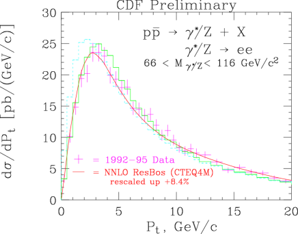
Figure 2: The $Z^{0}$ $p_{T}$ distribution (at low $p_{T}$) from CDF for Run 1 compared to predictions from ResBos and from PYTHIA. The two PYTHIA predictions use the default (rms) value for the non-perturbative $k_{T}$ (0.44 GeV) and the value that gives the best agreement with the shape of the data (2.15 GeV).

As stated previously, the resummed prediction correctly describes the shape of the $Z^{0}$ $p_{T}$ distribution at low $p_{T}$, although there is still a noticeable difference in shape between the Monte Carlo and the resummed prediction. It is interesting to note that if the process dependent coefficients ($B^{(1)}$ and $B^{(2)}$) were not incorporated into the resummation prediction, the result would be an increase in the height of the peak and a decrease in the rate between 10 and 20 GeV, leading to a better agreement with the PYTHIA prediction [115].

The PYTHIA and ResBos predictions both describe the data well over a wider $p_{T}$ range than shown in the figure. Note especially the agreement of PYTHIA with the data at high $p_{T}$, made possible by explicit matrix element corrections (from the subprocesses $q\overline{q}\to Z^{0}g$ and $gq\to Z^{0}q$) to the $Z^{0}$ production process.

4.4 Diphoton Production

Most of the comparisons between resummation calculations/Monte Carlos and data have been performed for Drell-Yan production, i.e. $q\overline{q}$ initial states. It is also interesting to examine diphoton production at the Tevatron, where a large fraction of the contribution at low diphoton mass is due to $gg$ scattering. The prediction for the di-photon $k_{T}$ distribution at the Tevatron, from PYTHIA (version 6.122), is shown in Figure 3, using the experimental cuts applied in the CDF analysis [116].

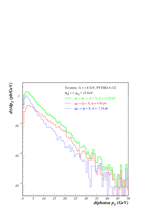
Figure 3: A comparison of the PYTHIA predictions for di-photon production at the Tevatron for the two different subprocesses, $q\overline{q}$ and $gg$. The same cuts are applied to PYTHIA as in the CDF di-photon analysis.

It is interesting to note that about half of the di-photon cross section at the Tevatron is due to the $gg$ subprocess, and that the di-photon $p_{T}$ distribution is noticeably broader for the $gg$ subprocess than the $q\overline{q}$ subprocess. The $gg$ subprocess predictions in ResBos agree well with those from PYTHIA while the $q\overline{q}$ $p_{T}$ distribution is noticeably broader in ResBos. The latter behavior is due to the presence of the $Y$ piece (fixed-order corrections) in ResBos at moderate $p_{T}$, and the matching of the $q\overline{q}$ cross section to the fixed order $q\overline{q}\to{\gamma}{\gamma}g$ at high $p_{T}$. The corresponding matrix element correction is not in PYTHIA. It is interesting to note that the PYTHIA and ResBos predictions for $gg\to{\gamma}{\gamma}$ agree in the moderate $p_{T}$ region, even though the ResBos prediction has the $Y$ piece present and is matched to the matrix element piece $gg\to{\gamma}{\gamma}g$ at high $p_{T}$, while there is no such matrix element correction for PYTHIA. This shows that the $Y$ piece correction is not important for the $gg$ subprocess, which is the same conclusion that was reached in Ref. [117]. This is probably a result of steep decline in the $gg$ parton-parton with increasing partonic center of mass energy, $\sqrt{\hat{s}}$. This falloff tends to suppress the size of the $Y$ piece since the production of the di-photon pair at higher $p_{T}$ requires larger $x_{1}$, $x_{2}$ values. In the default CSS formalism, there is no such kinematic penalty in the resummed piece since the soft gluon radiation comes for “free.” (Larger $x_{1}$ and $x_{2}$ values are not required.)

A comparison of the CDF di-photon data to NLO [118] and resummed (ResBos) QCD predictions has been performed, but the analysis is still in progress, so the results are not presented here. The transverse momentum distribution, in particular, is sensitive to the effects of the soft gluon radiation and better agreement can be observed with the ResBos prediction than with the NLO one. A much more precise comparison with the effects of soft gluon radiation will be possible with the 2 fb^-1 or greater data sample that is expected for both CDF and DØ in Run 2.

4.5 Higgs Boson Production

A comparison of the two versions of PYTHIA and of ResBos is shown in Figure 4 for the case of the production of a Higgs boson with mass 100 GeV at the Tevatron with center-of-mass energy of 2.0 TeV. The same qualitative features are observed at the LHC: the newer version of PYTHIA agrees better with ResBos in describing the low $p_{T}$ shape, and there is a falloff at high $p_{T}$ unless the hard scale for showering is increased. The default (rms) value of the non-perturbative $k_{T}$ (0.44 GeV) was used for the PYTHIA predictions. Note that the peak of the resummed distribution has moved to $p_{T}\approx$ 7 GeV (compared to about 3 GeV for $Z^{0}$ production at the Tevatron). This is due primarily to the larger color factors associated with initial state gluons ($C_{A}=3$) rather than quarks ($C_{F}=4/3$).

The newer version of PYTHIA agrees well with ResBos at low to moderate $p_{T}$, but falls below the resummed prediction at high $p_{T}$. This is easily understood: ResBos switches to the NLO Higgs + jet matrix element at high $p_{T}$ while the default PYTHIA can generate the Higgs $p_{T}$ distribution only by initial state gluon radiation, using as default a maximum scale equal to the Higgs boson mass. High $p_{T}$ Higgs boson production is another example where a $2\to 1$ Monte Carlo calculation with parton showering can not completely reproduce the exact matrix element calculation without the use of matrix element corrections. The high $p_{T}$ region is better reproduced if the maximum virtuality $Q_{max}^{2}$ is set equal to the collider center-of-mass energy, $s$, rather than subprocess $\hat{s}$. This is equivalent to applying the parton shower to all of phase space. However, the consequence is that the low $p_{T}$ region is now depleted of events, since the parton showering does not change the total production cross section. The appropriate scale to use in PYTHIA (or any Monte Carlo) depends on the $p_{T}$ range to be probed. If matrix element information is used to constrain the behavior, the correct high $p_{T}$ cross section can be obtained while still using the lower scale for showering. The incorporation of matrix element corrections to Higgs production (involving the processes $gq\to qH$,$q{\overline{q}}\to gH$, $gg\to gH$) is the next logical project for the Monte Carlo experts, in order to accurately describe the high $p_{T}$ region.

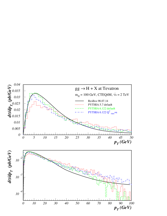
Figure 4: A comparison of predictions for the Higgs $p_{T}$ distribution at the Tevatron from ResBos and from two recent versions of PYTHIA. The ResBos and PYTHIA predictions have been normalized to the same area.

The older version of PYTHIA produces too many Higgs events at moderate $p_{T}$ (in comparison to ResBos) at both the Tevatron and the LHC. Two changes have been implemented in the newer version. The first change is that a cut is placed on the combination of $z$ and $Q^{2}$ values in a branching: $\hat{u}=Q^{2}/z-\hat{s}(1-z)<0$, where $\hat{s}$ refers to the subsystem of the hard scattering plus the shower partons considered to that point. The association with $\hat{u}$ is relevant if the branching is interpreted in terms of a $2\to 2$ hard scattering. This requirement is not fulfilled when the $Q^{2}$ value of the space-like emitting parton is little changed and the $z$ value of the branching is close to unity. This affects mainly the hardest emission (largest $Q^{2}$). The net result of this requirement is a substantial reduction in the total amount of gluon radiation [119]. Such branchings are kinematically allowed, but since matrix element corrections would assume initial state partons to have $Q^{2}=0$, a non-physical $\hat{u}$ results (and thus no possibility to impose matrix element corrections). The correct behavior is beyond the predictive power of leading log Monte Carlos.

In the second change, the parameter for the minimum gluon energy emitted in space-like showers is modified by an extra factor roughly corresponding to the $1/\gamma$ factor for the boost to the hard subprocess frame [119]. The effect of this change is to increase the amount of gluon radiation. Thus, the two effects are in opposite directions but with the first effect being dominant.

This difference in the $p_{T}$ distribution between the two versions of PYTHIA could have an impact on the analysis strategies for Higgs searches at the LHC. For example, for the CMS detector, the higher $p_{T}$ activity associated with Higgs production in version 5.7 would have allowed for a more precise determination of the event vertex from which the Higgs (decaying into two photons) originated. Vertex pointing with the photons is not possible in CMS, and the large number of interactions occurring with high intensity running will mean a substantial probability that at least one of the interactions will produce jets at low to moderate $E_{T}$. [120] In principle, this problem could affect the $p_{T}$ distribution for all PYTHIA processes. In practice, the effect has manifested itself only in $gg$ initial states, due to the enhanced branching probability.

As an exercise, an 80 GeV $W$ and an 80 GeV Higgs were generated at the Tevatron using PYTHIA5.7 [121]. A comparison of the distribution of values of $\hat{u}$ and the virtuality $Q$ for the two processes indicates a greater tendency for the Higgs virtuality to be near the maximum value and for there to be a larger number of Higgs events with positive $\hat{u}$ (than W events).

4.6 Comparison with HERWIG

The variation between versions 5.7 and 6.1 of PYTHIA gives an indication of the uncertainties due to the types of choices that can be made in Monte Carlos. The requirement that $\hat{u}$ be negative for all branchings is a choice rather than an absolute requirement. Perhaps the better agreement of version 6.1 with ResBos is an indication that the adoption of the $\hat{u}$ restrictions was correct. Of course, there may be other changes to PYTHIA which would also lead to better agreement with ResBos for this variable.

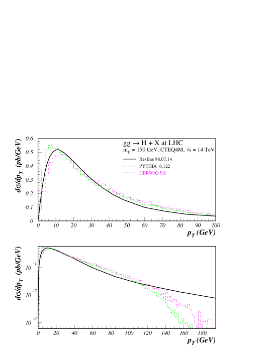
Figure 5: A comparison of predictions for the Higgs $p_{T}$ distribution at the LHC from ResBos, two recent versions of PYTHIA and HERWIG. The ResBos, PYTHIA and HERWIG predictions have been normalized to the same area.

Since there are a variety of choices that can be made in Monte Carlo implementations, it is instructive to compare the predictions for the $p_{T}$ distribution for Higgs boson production from ResBos and PYTHIA with that from HERWIG (version 5.6, also using the CTEQ4M parton distribution functions). The HERWIG prediction is shown in Figure 5 along with the PYTHIA and ResBos predictions, all normalized to the ResBos prediction.  In all cases, the CTEQ4M parton distribution was used. The predictions from HERWIG and PYTHIA 6.1 are very similar, with the HERWIG prediction matching the ResBos shape somewhat better at low $p_{T}$.

4.7 Non-perturbative $k_{T}$

A question still remains as to the appropriate value of non-perturbative $k_{T}$ to input in the Monte Carlos to achieve a better agreement in shape, both at the Tevatron and at the LHC. Figure 6 compares the ResBos and PYTHIA predictions for the Higgs boson $p_{T}$ distribution at the Tevatron. The PYTHIA prediction (now version 6.1 alone) is shown with several values of non-perturbative $k_{T}$. Surprisingly, no difference is observed between the predictions with the different values of $k_{T}$, with the peak in PYTHIA always being somewhat below that of ResBos. This insensitivity can be understood from the plots at the bottom of the two figures which show the sum of the non-perturbative initial state $k_{T}$ ($k_{T1}$+$k_{T2}$) at $Q_{0}$ and at the hard scatter scale $Q$. Most of the $k_{T}$ is radiated away, with this effect being larger (as expected) at the LHC. The large gluon radiation probability from a gluon-gluon initial state (and the greater phase space available at the LHC) lead to a stronger degradation of the non-perturbative $k_{T}$ than was observed with $Z^{0}$ production at the Tevatron.

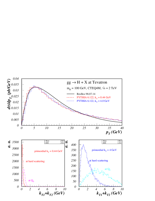
Figure 6: (top) A comparison of the PYTHIA predictions for the $p_{T}$ distribution of a 100 GeV Higgs at the Tevatron using the default (rms) non-perturbative $k_{T}$ (0.44 GeV) and a larger value (4 GeV), at the initial scale $Q_{0}$ and at the hard scatter scale. Also shown is the ResBos prediction (bottom) The vector sum of the intrinsic $k_{T}$ ($k_{T1}$+$k_{T2}$) for the two initial state partons at the initial scale $Q_{0}$ and at the hard scattering scale for the two values of intrinsic $k_{T}$.

4.8 Conclusions

An understanding of the signature for Higgs boson production at either the Tevatron or LHC depends upon the understanding of the details of soft gluon emission from the initial state partons. This soft gluon emission can be modeled either in a Monte Carlo or in a $k_{T}$ resummation program, with various choices possible in both implementations. A comparison of the two approaches is useful to understand the strengths and weaknesses of each. The data from the Tevatron that either exists now, or will exist in Run 2, will be extremely useful to test both approaches.

Acknowledgements

We would like to thank Claude Charlot, Gennaro Corcella, Willis Sakumoto, Torbjorn Sjöstrand and Valeria Tano for useful conversations and for providing some of the plots.

5 MCFM: a parton-level Monte Carlo at NLO Accuracy

by John Campbell and R.K. Ellis

5.1 Introduction

In Run II, experiments at the Tevatron will be sensitive to processes occurring at the femtobarn level. Of particular interest are processes which involve heavy quarks, leptons and missing energy, since so many of the signatures for physics beyond the standard model produce events containing these features. We have therefore written the program MCFM [123, 79] which calculates the rates for a number of standard model processes. These processes are included beyond the leading order in the strong coupling constant where possible; in QCD this is the first order in which the normalization of the cross sections is determined. Because the program produces weighted Monte Carlo events, we can implement experimental cuts allowing realistic estimates of event numbers for an ideal detector configuration. MCFM is expected to give more reliable results than parton shower Monte Carlo programs, especially in phase space regions with well separated jets. On the other hand it gives little information about the phase space regions which are dominated by multiple parton emission. In addition, because the final state contains partons rather than hadrons, a full detector simulation cannot be performed directly using the output of MCFM.

The processes already included in MCFM at NLO are as follows ($H_{1},H_{2}=p$ or $\bar{p}$),

• $H_{1}+H_{2}\rightarrow W^{\pm}$

• $H_{1}+H_{2}\rightarrow Z$

• $H_{1}+H_{2}\rightarrow W^{\pm}+\mbox{1 jet}$

• $H_{1}+H_{2}\rightarrow Z+\mbox{1 jet}$

• $H_{1}+H_{2}\rightarrow W^{\pm}+H$

• $H_{1}+H_{2}\rightarrow Z+H$

• $H_{1}+H_{2}\rightarrow W^{+}W^{-}$

• $H_{1}+H_{2}\rightarrow W^{\pm}Z$

• $H_{1}+H_{2}\rightarrow ZZ$

• $H_{1}+H_{2}\rightarrow W^{+}+g^{*}(\rightarrow b\bar{b}),~{}\mbox{massless}~{}$b-quarks

• $H_{1}+H_{2}\rightarrow Z+g^{*}(\rightarrow b\bar{b}),~{}\mbox{massless}~{}$b-quarks

• $H_{1}+H_{2}\rightarrow H\rightarrow W^{+}W^{-},ZZ~{}\mbox{or}~{}t\bar{t}$

• $H_{1}+H_{2}\rightarrow\tau^{+}+\tau^{-}\;.$

The decays of vector bosons and/or Higgs bosons are included. We have also included the leptonic decays of the $\tau$-lepton. As described below the implementation of NLO corrections requires the calculation of both the amplitude for real radiation and the virtual corrections to the Born level process. We have extensively used the one loop results of Bern, Dixon, Kosower et al. [124], [125] to obtain the virtual corrections to above processes.

A future development path for the program would be to include the following processes at NLO:

• $H_{1}+H_{2}\rightarrow W^{\pm}+\mbox{2 jets}$

• $H_{1}+H_{2}\rightarrow Z+\mbox{2 jets}\;.$

In addition there are an number of processes which we have included only at leading order. This restriction to leading order is both a matter of expediency and because the theoretical framework for including radiative corrections to processes involving massive particles is not yet complete.

• $H_{1}+H_{2}\rightarrow t+\bar{t}$

• $H_{1}+H_{2}\rightarrow t+\bar{t}+\mbox{1 jet}$

• $H_{1}+H_{2}\rightarrow t+\bar{b}$

• $H_{1}+H_{2}\rightarrow t+\bar{b}+\mbox{1 jet}$

• $H_{1}+H_{2}\rightarrow t+\bar{t}+H$

• $H_{1}+H_{2}\rightarrow t+\bar{t}+Z$

$H,Z$ and top quark decays are included.

5.2 General structure

In order to evaluate the strong radiative corrections to a given process, we have to consider Feynman diagrams describing real radiation, as well as the diagrams involving virtual corrections to the tree level graphs. The corrections due to real radiation are dealt with using a subtraction algorithm[126] as formulated by Catani and Seymour [127]. This algorithm is based on the fact that the singular parts of the QCD matrix elements for real emission can be singled out in a process-independent manner. By exploiting this observation, one can construct a set of counter-terms that cancel all non-integrable singularities appearing in real matrix elements. The NLO phase space integration can then be performed numerically in four dimensions.

The counter-terms that were subtracted from the real matrix elements have to be added back and integrated analytically over the phase space of the extra emitted parton in $n$ dimensions, leading to poles in $\epsilon=(n-4)/2$. After combining those poles with the ones coming from the virtual graphs, all divergences cancel, so that one can safely perform the limit $\epsilon\rightarrow 0$ and carry out the remaining phase space integration numerically.

As an example of this procedure we consider the production of an on-shell $W$ boson decaying to a lepton-antilepton pair.

$$q(p_{1})+\bar{q}(p_{2})\rightarrow W^{+}(\nu(p_{3})+e^{+}(p_{4})),\\[2.84526pt] p_{1}+p_{2}=p_{3}+p_{4},\;\;(p_{3}+p_{4})^{2}=M_{W}^{2}.$$ (18)

In this case, the $W$ boson rapidity distribution is calculable analytically in $O(\alpha_{s})$ [128, 129]. Fig. 7 shows the result calculated in the $\overline{MS}$ scheme.

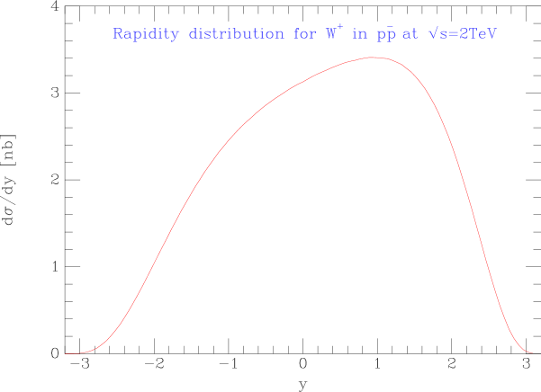
Figure 7: The rapidity distribution for $W^{+}$ production in $p\bar{p}$ collisions at $\sqrt{s}=2\mbox{TeV}$.

The virtual corrections to (18) are of the Drell-Yan type and are well known [128]. They are expressible as an overall factor multiplying the lowest order matrix element squared,

$$\sigma^{\rm V}=\sigma^{\rm LO}\times\frac{\alpha_{s}C_{F}}{2\pi}\left(\frac{4\pi\mu^{2}}{Q^{2}}\right)^{\epsilon}\frac{1}{\Gamma(1-\epsilon)}\\[2.84526pt] \left[-\frac{2}{\epsilon^{2}}-\frac{3}{\epsilon}-6+\pi^{2}\right]$$ (19)

and must be combined with the real radiation contribution. For example, gluon radiation from the $q\bar{q}$ initial state yields the subprocess

$$q(p_{1})+\bar{q}(p_{2})\rightarrow W(\nu(p_{3})+e^{+}(p_{4}))+g(p_{5}),\\[2.84526pt] p_{1}+p_{2}=p_{3}+p_{4}+p_{5}.$$ (20)

To eliminate the singular part of this subprocess, we generate a counter event with the kinematics of the $2\to 2$ process as follows

$$q(x_{a}p_{1})+\bar{q}(p_{2})\rightarrow W(\nu(\tilde{p}_{3})+e^{+}(\tilde{p}_{4})),\\[2.84526pt] x_{a}p_{1}+p_{2}=\tilde{p}_{3}+\tilde{p}_{4}$$ (21)

where a Lorentz transformation has been performed on all $j$ final state momenta

$$\tilde{p}^{\mu}_{j}=\Lambda^{\mu}_{\nu}p_{j}^{\nu},\;\;j=3,4$$ (22)

such that $\tilde{p}_{j}^{\mu}\rightarrow p_{j}$ for $p_{5}$ collinear or soft. Thus the energy of the emitted gluon $p_{5}$ is absorbed by $p_{1}$, and the momentum components are absorbed by the transformation of the final state vectors. The phase space has a convolution structure,

$$d\Phi^{(3)}(p_{5},p_{4},p_{3};p_{2},p_{1})=\\[2.84526pt] \int_{0}^{1}dx\,d\Phi^{(2)}(\tilde{p}_{4},\tilde{p}_{3};p_{2},p_{1})\times[dp_{5}(p_{1},p_{2},x)]$$ (23)

where

$$[dp_{5}(p_{1},p_{2},x)]=\\[2.84526pt] \frac{d^{d}p_{5}}{(2\pi)^{d-1}}\,\delta^{+}(p_{5}^{2})\Theta(x)\Theta(1-x)\delta(x-x_{a})$$ (24)

This phase space may be used to integrate out the dipole term $D^{15,2}$, which is chosen to reproduce the singularities in the real matrix elements as the gluon ($5$) becomes soft or collinear to the quark ($1$),

$$D^{15,2}=\frac{4\pi\alpha_{s}C_{F}\mu^{2\epsilon}}{p_{1}\cdot p_{5}}\left(\frac{2}{1-x_{a}}-1-x_{a}\right)$$ (25)

Performing the integration yields,

$$\int_{0}^{1}dx\,D^{15,2}\,[dp_{5}(p_{1},p_{2},x)]=$$

$$\frac{\alpha_{s}C_{F}}{2\pi}\left(\frac{4\pi\mu^{2}}{2p_{1}\cdot p_{2}}\right)^{\epsilon}\frac{1}{\Gamma(1-\epsilon)}\times$$

$$\left[-\frac{1}{\epsilon}p_{qq}(x)+\delta(1-x)\left(\frac{1}{\epsilon^{2}}+\frac{3}{2\epsilon}-\frac{\pi^{2}}{6}\right)\right.$$

$$\left.+2(1+x^{2})\left[\frac{\log(1-x)}{1-x}\right]_{+}\right]$$ (26)

with the Altarelli-Parisi function $p_{qq}(x)$ given by

$$p_{qq}(x)=\frac{2}{(1-x)_{+}}-1-x+\frac{3}{2}\delta(1-x)$$ (27)

In order to obtain the complete counter-term, one must add the (identical) contribution from the dipole configuration $D^{25,1}$ that accounts for the gluon becoming collinear with the anti-quark. In a more complicated process, we would sum over a larger number of distinct dipole terms involving partons both in the initial and final states. In this simple case, we find the total counter-term contribution to the $q{\bar{q}}$ cross-section to be

$$\sigma^{\rm CT}=\frac{\alpha_{s}C_{F}}{2\pi}\left(\frac{4\pi\mu^{2}}{Q^{2}}\right)^{\epsilon}\frac{1}{\Gamma(1-\epsilon)}\times\Biggl{[}\Biggr{.}$$

$$\Biggl{.}-\frac{2}{\epsilon}p_{qq}(x)+\delta(1-x)\left(\frac{2}{\epsilon^{2}}+\frac{3}{\epsilon}-\frac{\pi^{2}}{3}\right)$$

$$-2p_{qq}(x)\log x+4(1+x^{2})\left[\frac{\log(1-x)}{1-x}\right]_{+}\Biggr{]}$$

where each of these terms leads to a different type of contribution in MCFM. The first term, proportional to $p_{qq}(x)$, is canceled by mass factorization, up to some additional finite (${\cal O}(\epsilon^{0})$) pieces. The terms multiplying the delta-function $\delta(1-x)$ manifestly cancel the poles generated by the virtual graphs, given in equation (19), leaving an additional $\pi^{2}$ contribution. The remaining terms, which don’t have the structure of the virtual contribution, are collected together and added separately in MCFM.

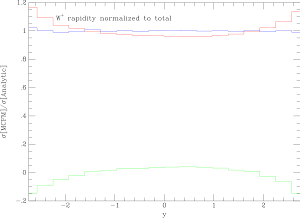
Figure 8: The ratio of the contributions to the rapidity distribution of $W^{+}$ production

In Fig. 8 we have plotted the three contributions to the $W$ rapidity calculated using MCFM. The three contributions are $a$) the contribution of (real-counterterm) [the lower curve], $b$) the contribution of leading order + virtual + integrated counter-term [the upper-most curve] and $c$) the total contribution. All three terms have been normalized to the $O(\alpha_{s})$ rapidity distribution shown in Fig. 7. We see that ($b$), the leading order term, combined with the virtual correction and the results from the counterterm provides the largest contribution to the cross section. The total contribution is a horizontal line at unity, showing the agreement between MCFM and the analytically calculated result. Only at the boundaries of the phase space at large $y$ can the contribution of the real emission minus the counterterm become sizeable.

5.3 Examples of MCFM results

We first detail the input parameters used in our phenomenological estimates. The electroweak theory is specified by four numbers, $M_{W},M_{Z},\alpha(M_{Z})$, and $G_{F}$, the values of which are given in Table 1, together with other necessary constants. Other derived parameters are $e,g_{W}$ and $\sin^{2}\theta_{W}$ which, when defined as below, are effective parameters including the leading effects of top quark loops[130]. We use the the first of the MRS99 parton distributions[131] which has $\alpha_{S}(M_{Z})=0.1175$.

$$e^{2} = 4\pi\alpha(M_{Z})$$

$$g^{2}_{W} = 4\sqrt{2}G_{F}M_{W}^{2}$$

$$\sin^{2}\theta_{W} = \frac{e^{2}}{g^{2}_{W}}$$ (28)

Table 1: Input parameters

$M_{Z},\Gamma_{Z}$	$91.187,2.49~{}\mbox{GeV}$
$M_{W},\Gamma_{W}$	$80.41,2.06~{}\mbox{GeV}$
$m_{t},\Gamma_{t}$	$175,1.4~{}\mbox{GeV}$
$\alpha(M_{Z})$	1/128.89
$G_{F}$	$1.16639\times 10^{-5}$
$\sin^{2}\theta_{W}$	0.228534483
$V_{ud}$	0.97500
$V_{us}$	0.22220
$V_{cd}$	0.22220
$V_{cs}$	0.97500
Higgs mass (GeV)	BR($H\to b\bar{b}$)
$100$	$0.8119$
$110$	$0.7697$
$120$	$0.6778$
$130$	$0.5254$

Table 2: Diboson cross sections (in pb) at the Tevatron and the LHC

$\sqrt{s}$	$\sigma(W^{+}W^{-})$	$\sigma(W^{+}Z)$	$\sigma(W^{-}Z)$	$\sigma(ZZ)$
$2~{}\mbox{TeV}~{}(p\bar{p})$	$12.2$	$2.02$		$1.75$
$14~{}\mbox{TeV}~{}(pp)$	$103.6$	$27.2$	$17.7$	$16.7$

Table 2 shows the production cross sections for di-boson production calculated using MCFM for $p\bar{p}$ collisions at $\sqrt{s}=2$ TeV and for $pp$ collisions at $\sqrt{s}=14$ TeV. The next-to-leading order corrections vary between approximately $30\%$ and $50\%$ of leading order and are almost entirely due to the virtual graphs. The numbers here are slightly different than the results in [79], because of the different choices made both for the input EW parameters and parton distributions as detailed above.

Much effort has been devoted to the study of Higgs production at the Tevatron at $\sqrt{s}=2$ TeV. These studies indicate that, given enough luminosity, a light Higgs boson can be discovered at the Tevatron using the associated production channels $WH$ and $ZH$. In this report we present results of an analysis that incorporates as many of the backgrounds as possible at next-to-leading order for the $WH$ channel. Whilst we use no detector simulation and do not attempt to include non-physics backgrounds, the results presented here can provide a normalization for more detailed studies. This is of importance since more detailed studies are often performed using shower Monte Carlo programs which can give misleading results for well separated jets.

In particular, we will consider the light Higgs case ($M_{H}<130$ GeV) in the channel $p\bar{p}\rightarrow b\bar{b}\nu e^{+}$. In addition to the usual cuts on rapidity and transverse momentum,

$$\begin{array}[]{rcl}|y_{b}|,|y_{\bar{b}}|&<&2\ ,\\ |y_{e}|&<&2.5\ ,\\ |p^{T}_{b}|,|p^{T}_{\bar{b}}|&>&15~{}\mbox{GeV}\ ,\\ |p^{T}_{e}|,|p^{T}_{\nu}|&>&20~{}\mbox{GeV}\ ,\end{array}$$ (29)

we also impose isolation cuts,

$$R_{b\bar{b}},R_{eb},R_{e\bar{b}}>0.7\ ,$$ (30)

as well as a cut on the scattering angle of the $b\bar{b}$ system [132] (the Higgs scattering angle) in the Collins-Soper frame [133],

$$|\cos{\theta_{b\bar{b}}}|<0.8\ .$$ (31)

Note that imposing the cut on $\cos{\theta_{b\bar{b}}}$ requires knowledge of the longitudinal component of a neutrino momentum. Our results for the signal, backgrounds and significance are shown in Table 3, where we use $\epsilon_{b{\bar{b}}}=0.45$ and integrate the cross-sections over a $b{\bar{b}}$ mass range appropriate for the Higgs mass under consideration,

$$|M_{H}-M_{b\bar{b}}|<\sqrt{2}\sigma_{M},\sigma_{M}=.1M_{H}.$$ (32)

Table 3: Signal, backgrounds (in fb) and significance for the $W$-channel at $\sqrt{s}=2~{}\mbox{TeV}$

$M_{H}$ [GeV]	Scale	100	110	120	130
$W^{\pm}H(\rightarrow b\bar{b})$	$m_{H}$	$8.8$	$6.4$	$4.2$	$2.5$
$W^{\pm}g^{*}(\rightarrow b\bar{b})$	$(m_{W}+100~{}\mbox{GeV})/2$	$25.7$	$22.7$	$18.5$	$15.5$
$W^{\pm}Z(\rightarrow b\bar{b})$	$(m_{W}+100~{}\mbox{GeV})/2$	$6.7$	$4.3$	$2.0$	$1.0$
$t(\rightarrow bW^{+})\bar{t}(\rightarrow\bar{b}W^{-}_{\rm lept})$	$100~{}\mbox{GeV}$	$3.3$	$3.7$	$3.9$	$3.9$
$t(\rightarrow bW^{+})\bar{t}(\rightarrow\bar{b}W^{-}_{\rm hadr})$	$100~{}\mbox{GeV}$	$0.3$	$0.4$	$0.5$	$0.6$
$W^{\pm*}(t(\rightarrow bW^{+})\bar{b})$	$100~{}\mbox{GeV}$	$5.1$	$5.8$	$6.0$	$6.0$
$q^{\prime}t(\rightarrow bW^{+})$	$100~{}\mbox{GeV}$	$0.3$	$0.4$	$0.5$	$0.6$
Total $B$	-	$41.4$	$37.3$	$31.4$	$27.6$
$S/B$	-	$0.21$	$0.17$	$0.13$	$0.09$
$S/\sqrt{B}$	-	$1.37$	$1.05$	$0.75$	$0.48$

From this table, one can see that, even with a fairly restrictive set of cuts, the $Wg^{*}$ process in particular provides a challenging background. This is further emphasized in Figure 9, where the cross-sections for $M_{H}=110$ GeV are presented in $5$ GeV bins across the entire $m_{b{\bar{b}}}$ spectrum. The signal, the two largest backgrounds and the sum of all the backgrounds including top quark production are plotted separately, as well as the totals with and without the Higgs signal.

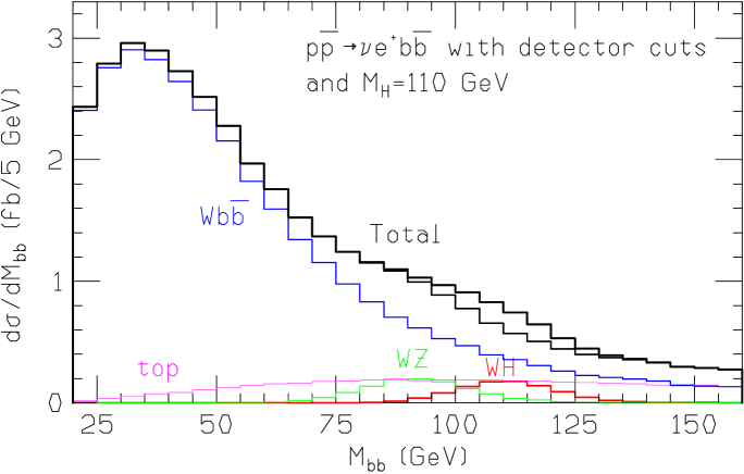
Figure 9: Signal and backgrounds for WH. ‘top’ represents the sum of all the backgrounds including a top quark.

The sharp peak of the Higgs signal becomes only a small shoulder in the total distribution.

5.4 Conclusions

We have introduced the program MCFM, which calculates the rates for a number of standard model processes that are particularly relevant in Run II. These calculations are performed in fixed-order perturbation theory, mainly at next-to-leading order in the strong coupling, and as such differ from other approaches such as parton shower Monte Carlos. As illustrations of the use of MCFM, we have presented total di-boson cross-sections and a primitive study (lacking detector effects and non-physics backgrounds) of $WH$ production as a search for a light Higgs. Such calculations can be used to provide normalizations for more detailed studies in the future.

6 Experimental handles on the backgrounds to new physics searches

by Regina Demina

6.1 Introduction

Significant work has been done in the course of the SUSY/Higgs [64] and Strong Dynamics [65] Workshops to understand the Tevatron discovery potential for new physics. Several promising signatures have been identified and the discovery reach has been estimated. In these studies, it was assumed that the systematic error on the signal and background normalization is similar in size to the statistical error, which is about 10%. Thus, the systematic error of each individual background process must be kept under 5%. Though it is probably a reasonable assumption, this will not happen automatically and dedicated studies are needed to achieve this goal. In this paper, we review the most important backgrounds to new physics and ways to estimate them in signal-depleted control samples.

6.2 New physics signatures

Associated vector boson and heavy flavor jets production is probably the most promising signature for new physics searches at the Tevatron. Standard Model (SM) Higgs boson [66], Supersymmetry [67], technicolor and topcolor [68] and even extra-dimension [69] signatures may appear in these channels.

#	Process	Model	Special features
1	$WH,H\to b\bar{b}$	SM Higgs	Resonance in $M_{b\bar{b}}$
2	$\rho_{T}^{\pm}\to W^{\pm}\pi_{T}^{0},\pi_{T}^{0}\to b\bar{b}$	Technicolor	Resonance in $M_{Wb\bar{b}}$ and $M_{b\bar{b}}$
3	$\rho_{T}^{0}\to W^{\pm}\pi_{T}^{\mp},\pi_{T}^{\pm}\to c\bar{b}$	Technicolor	Resonance in $M_{Wc\bar{b}}$ and $M_{c\bar{b}}$
4	$\widetilde{\chi}^{+}_{1}\widetilde{\chi}^{0}_{2},\widetilde{\chi}^{+}_{1}\to\ell\nu\widetilde{\chi}^{0}_{1},\widetilde{\chi}^{0}_{2}\to b\bar{b}\widetilde{\chi}^{0}_{1}$	SUSY	$M_{T}(\ell\hbox to0.0pt{\hbox to7.95831pt{\hfil/\hfil}\hss}E_{T})$ inconsistent with $W$
5	$t\bar{t},t\to bW,\bar{t}\to\widetilde{\bar{t}}\widetilde{\chi}^{0}_{1},\widetilde{\bar{t}}\to c\widetilde{\chi}^{0}_{1}$	SUSY	$M_{T}(\ell\hbox to0.0pt{\hbox to7.95831pt{\hfil/\hfil}\hss}E_{T})$ inconsistent with $W$

Table 4: Potential new physics signatures in the $W+2$ jet channel. From the experimental point of view, a “$W$” is a high $p_{T}$ lepton accompanied by significant missing energy (e.g., CDF cuts are $p_{T}(e,\mu)>20$ GeV/c, $\hbox to0.0pt{\hbox to7.95831pt{\hfil/\hfil}\hss}E_{T}>20$ GeV). In that sense, $\widetilde{\chi}^{+}_{1}$ looks like a “$W$.”

#	Process	Model	Special features
1	$t\bar{t},t\to bW,\bar{t}\to\widetilde{\bar{t}}\widetilde{\chi}^{0}_{1},\widetilde{\bar{t}}\to\bar{b}\widetilde{\chi}^{-}_{1}$	SUSY	$M_{T}(\ell\hbox to0.0pt{\hbox to7.95831pt{\hfil/\hfil}\hss}E_{T})$ inconsistent with $W$
2	$\tilde{t}\widetilde{\bar{t}},\tilde{t}\to b\widetilde{\chi}^{+}_{1}$	SUSY	$M_{T}(\ell\hbox to0.0pt{\hbox to7.95831pt{\hfil/\hfil}\hss}E_{T})$ inconsistent with $W$
3	$\tilde{t}\widetilde{\bar{t}},\tilde{t}\to b\ell\tilde{\nu}$	SUSY	$M_{T}(\ell\hbox to0.0pt{\hbox to7.95831pt{\hfil/\hfil}\hss}E_{T})$ inconsistent with $W$
4	$\widetilde{g}\widetilde{g},\widetilde{g}\to t\tilde{\bar{t}}$	SUSY	$M_{T}(\ell\hbox to0.0pt{\hbox to7.95831pt{\hfil/\hfil}\hss}E_{T})$ inconsistent with $W$
5	$Z^{\prime}(V_{8},\eta_{t})\to t\bar{t}$	Topcolor	Resonance in $M_{t\bar{t}}$

Table 5: Potential new physics signatures in the $W+3$ or more jet channel.

Tables 4 and 5, show examples of new physics processes that can produce $W+2$ jet and $W+3$ or more jet signatures. From the experimental point of view, a “$W$” is usually a high $p_{T}$ lepton accompanied by a significant missing energy (e.g. CDF Run I cuts are $P_{T}(e,\mu)>20$ GeV/c, $\hbox to0.0pt{\hbox to7.95831pt{\hfil/\hfil}\hss}E_{T}>20$ GeV [70]). In that sense, the supersymmetric partner of $W$ – $\widetilde{\chi}^{+}_{1}$ – looks like a $W$, except its transverse mass will be inconsistent with the $W$ hypothesis, but this will become obvious only when significant statistics is accumulated. Some models predict special features, like resonance behavior in the $b\bar{b}$ invariant mass, while others do not.

#	Process	Model	Special features
1	$ZH,H\to b\bar{b}$	SM Higgs	Resonance in $M_{b\bar{b}}$
2	$\rho_{T}^{+}\to Z\pi_{T}^{+},\pi_{T}^{+}\to c\bar{b}$	Technicolor	Resonance in $M_{Zc\bar{b}}$ and $M_{c\bar{b}}$
3	$\widetilde{\chi}^{+}_{1}\widetilde{\chi}^{0}_{2},\widetilde{\chi}^{+}_{1}\to c\bar{s}\widetilde{\chi}^{0}_{1},\widetilde{\chi}^{0}_{2}\to\ell^{+}\ell^{-}\widetilde{\chi}^{0}_{1}$	SUSY	$M_{\ell\ell}$ inconsistent with $Z$, extra $\hbox to0.0pt{\hbox to7.95831pt{\hfil/\hfil}\hss}E_{T}$
4	$\tilde{b}\widetilde{\bar{b}},\tilde{b}\to b\widetilde{\chi}^{0}_{1},\widetilde{\bar{b}}\to\bar{b}\widetilde{\chi}^{0}_{2},\widetilde{\chi}^{0}_{2}\to\ell\ell\widetilde{\chi}^{0}_{1}$	SUSY	extra $\hbox to0.0pt{\hbox to7.95831pt{\hfil/\hfil}\hss}E_{T}$

Table 6: Potential new physics signatures in the $Z+2$ jet channel. From the experimental point of view, a “$Z$” is two high $p_{T}$ leptons, usually with a $Z$ mass window cut. In that sense, $\widetilde{\chi}^{0}_{2}$ looks like a “$Z$” only in some regions of SUSY parameter space.

#	Process	Model	Special features
1	$\tilde{t}\widetilde{\bar{t}},\tilde{t}\to c\widetilde{\chi}^{0}_{1}$	SUSY	2 charm jets and $\hbox to0.0pt{\hbox to7.95831pt{\hfil/\hfil}\hss}E_{T}$
1	$\tilde{b}\widetilde{\bar{b}},\tilde{b}\to b\widetilde{\chi}^{0}_{1}$	SUSY	2 bottom jets and $\hbox to0.0pt{\hbox to7.95831pt{\hfil/\hfil}\hss}E_{T}$
3	$LQ_{2}LQ_{2},LQ_{2}\to c\nu$	Leptoquarks	2 charm jets and $\hbox to0.0pt{\hbox to7.95831pt{\hfil/\hfil}\hss}E_{T}$
3	$LQ_{3}LQ_{3},LQ_{3}\to b\nu$	Leptoquarks	2 bottom jets and $\hbox to0.0pt{\hbox to7.95831pt{\hfil/\hfil}\hss}E_{T}$

Table 7: Potential new physics signatures in the $\hbox to0.0pt{\hbox to7.95831pt{\hfil/\hfil}\hss}E_{T}+2$ jet channel. This does not include processes complementary to those in Table 6, where a $Z$ decays to a pair of neutrinos $Z\to\nu\bar{\nu}$, thus producing missing energy.

Table 6 presents new physics processes that can produce $Z+2$ jet signatures. Here we assume that the $Z$ decays to a pair of leptons. Usually, a $Z$ mass window cut is applied. In that sense, the supersymmetric partner of the $Z$ – $\widetilde{\chi}^{0}_{2}$ – looks like a $Z$ in only some regions of SUSY parameter space. If the $Z$ decays to a pair of neutrinos, it produces missing energy. In this case, all the processes presented in Table 6 produce a $\hbox to0.0pt{\hbox to7.95831pt{\hfil/\hfil}\hss}E_{T}+2$ jet signature. Table 7 shows additional new physics processes that result in a $\hbox to0.0pt{\hbox to7.95831pt{\hfil/\hfil}\hss}E_{T}$ signature. As we see, these channels are very important for new physics searches, and the Standard Model backgrounds to these signatures must be thoroughly understood before any claims of discovery are made.

6.3 Backgrounds to new physics

The $W(Z)b\bar{b}$ signature was studied in the course of the SUSY/Higgs Workshop for the Higgs discovery potential estimate [66]. The $\hbox to0.0pt{\hbox to7.95831pt{\hfil/\hfil}\hss}E_{T}$+heavy flavor $(c/b)$ signature was studied in the CDF stop/sbottom search [71]. We use these analyses as examples in our discussion.

$W(Z)b\bar{b}$ signature

Selection and sample composition

The $Wb\bar{b}$ ($Z(\to\nu\bar{\nu})b\bar{b}$) selection criteria and the resultant sample composition are summarized in Fig. 10 (Fig. 11). The dominant contribution to both samples is QCD production of a vector boson accompanied by two $b$-jets.

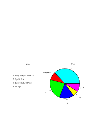
Figure 10: Selection cuts and composition of the $Wb\bar{b}$ sample.

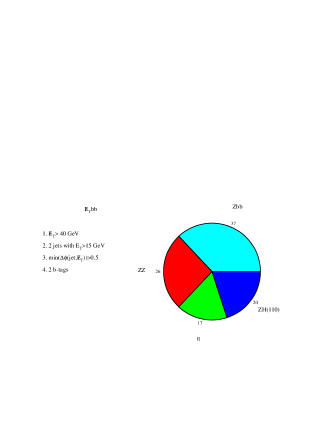
Figure 11: Selection cuts and composition of the $\hbox to0.0pt{\hbox to7.95831pt{\hfil/\hfil}\hss}E_{T}b\bar{b}$ sample.

QCD $W(Z)b\bar{b}$ production. Experimental studies of gluon splitting to heavy flavor.

Diagrams of QCD associated production of $W(Z)$ and heavy flavor jets are presented in Figure 12. The leading contribution is $W(Z)$+gluon production with subsequent gluon splitting to a $b\bar{b}$ or $c\bar{c}$ pair, shown in Figure 12(a).

Figure 12: Diagrams of QCD associated production of $W(Z)$ and heavy flavor jets.

Though a next-to-leading-order calculation of the QCD $Wb\bar{b}$ production exists [72], even the authors themselves recommend that it should be tested experimentally. This is a particularly hard task in the presence of a potential signal contribution. In the case of the Higgs search, an invariant mass of two $b$-jets could be used as an additional handle, since gluon splitting contributes mainly to the low part of the $M_{b\bar{b}}$ spectrum, while the Higgs is a resonance at 110-130 GeV/c². This is not the case for some other potential signal process, e.g. process 5 in Table 4.

The probability for a gluon to split to two heavy flavor jets can be studied experimentally in different samples. The signal contamination becomes negligible, if the presence of a vector boson is not required.

Three heavy flavor production mechanisms can be isolated – direct production, final state gluon splitting and initial state gluon splitting, also called flavor excitation. Diagrams of these processes are presented in Figure 13.

Figure 13: Diagrams of QCD heavy flavor production.

Though direct production is the lowest order process, it is responsible for the production of only $\sim~{}20$% of heavy flavor jets with energy above 20 GeV; about 35% are produced by flavor excitation and 45% by gluon splitting. The relative contribution of different processes changes after $b$-tagging is applied. Tagging is usually more efficient on directly produced jets, which tend to be back-to-back in the azimuthal plane. Heavy flavor quarks produced from gluon splitting are not well separated, and are often assigned to the same jet. Thus the relative contribution of gluon splitting to the double-tagged jet sample is quite low. Flavor excitation involves an initial state gluon splitting to two heavy flavor quarks, one of which undergoes hard scattering. The other quark, being a part of the proton remnant, is often outside the detector acceptance. Thus, the contribution of flavor excitation to the double-tagged sample is significantly depleted. An analysis of the angular correlation between two heavy flavor tagged jets can be used to isolate the gluon-splitting component in heavy flavor production, as depicted in Fig. 14.

Figure 14: Distribution $\Delta\phi$ between two $b$-quarks from Monte Carlo events.

Different methods can be used to tag heavy flavor jets.

1. Impact parameter or secondary vertex tagging (JETPROB or SECVTX in CDF jargon) [70] are the ones most commonly used. These samples have relatively high statistics. Using the same tagging method for the background and the signal sample eliminates the systematic uncertainty. The main disadvantage of these methods is the relatively low purity of these samples – contamination from $c$-jets and mistags is non-negligible. Usually, to get a stable fit, the $b/c$ ratio has to be fixed to the one predicted by Monte Carlo, which is not without its own uncertainty.

2. One of the heavy flavor jets is tagged by the presence of a high $p_{T}>8$ GeV/c lepton – electron or muon – and JETPROB or SECVTX tags another jet [73]. These samples have high statistics as well, but again suffer from charm and mistag contamination. Nonetheless, it is an interesting independent study.

3. Both heavy flavor jets can be tagged by leptons. In this case it is possible to go lower in lepton momentum, usually $p_{T}>3$ GeV/c [74]. Compared to the first two cases, these studies probe a lower energy region, where the direct production mechanism dominates. Thus not much information about gluon splitting probability can be gained.

4. Study #2 can be modified to increase the purity by reconstructing exclusive or semi-exclusive final states in one of the jets:

   1. Reconstructing a decay chain $D^{*}\to D^{0}\pi,D^{0}\to Ke(\mu)\nu$ can isolate the charm contribution [75]. The presence of a high $p_{T}$ lepton guarantees that the contribution from $b\to c$ decay is at the order of 10% or lower. Studying the angular correlation between $D^{*}$ jet and an impact parameter tagged jet isolates the gluon splitting to charm contribution. This probability can then be applied to study #2 to extract the probability of gluon splitting to $b$-quarks.

   2. A similar trick can be used to isolate the $b$-contribution in the lepton sample. Promising decay chains are [76]: $B\to\ell\nu D^{*}$, $D^{*}\to D^{0}\pi$, $D^{0}\to K\pi$ or $K3\pi$; $B\to\ell\nu D^{+}$, $D^{+}\to K\pi\pi$; $B\to\ell\nu D^{0}$, $D^{0}\to K\pi$; and $B\to J/\Psi K$.

#	Sample	N(Run I)	$\sigma(g\to Q\bar{Q})$ Run I	N(Run II)	$\sigma(g\to Q\bar{Q})$ Run II
1	Double tagged jets	700	20%	28000	3.2%
2	Muon+JETPROB tag	2620	16%	104800	2.5%
3	$c\to D^{*}\to D^{0}(\to K\ell\nu)\pi$	18000	15%	720000	2.4%
4	$B\to D^{*}\ell\nu\to D^{0}(\to K\pi/K3\pi)\ell\nu\pi$	1700	n.a.	68000	n.a.
5	$B\to D^{+}(\to K\pi\pi)\ell\nu$	1900	n.a.	76000	n.a.
6	$B\to D^{0}(\to K\pi)\ell\nu$	2700	#4-#7	108000	#4-#7
7	$B\to J/\Psi K^{(*)}$	1300	23%	52000	3.6%

Table 8: Data samples for heavy flavor production study. Numbers in samples #1 and #2 are double tags, while in samples #3-#7 numbers of exclusively reconstructed events are shown, without requiring a tag on the opposite side.

In Table 8, we present the number of events in each of the discussed samples collected in Run I and expected in Run II and associated statistical uncertainty on the gluon splitting probability.

Run I numbers are based on CDF results. In Run II, both CDF and DØ will have similar tracking and vertexing capabilities, thus these numbers are applicable to both detectors. Statistics in Run II is increased by a factor of 40, where 20 is gained from the luminosity increase and 2 from increased acceptance of the silicon microvertex detectors. The tagging efficiency increase is not taken into account. With these dedicated studies, the statistical uncertainty on the probability of gluon splitting to heavy flavor quarks can be significantly reduced in Run II, and will become adequate to the needs of new physics searches.

Top, single top and diboson production

Other backgrounds to new physics searches are top pair [77], single top [78] and diboson [79] production. The theoretical predictions for these backgrounds are more reliable, because they do not involve gluon radiation and splitting, yet they still have to be tested experimentally. This is more or less a straightforward task for top pair and diboson production, where final states can be exclusively identified. It is less so for single top production, where the final state is exactly the same – $Wb\bar{b}$ – as in new physics channels in Table 4. Additional mass constraints, e.g. on the $Wb$ mass can be used to isolate this process, but it is not at all obvious that adequate uncertainty can be reached for this channel.

Missing energy and heavy flavor signatures

Here, we summarize the selection criteria and composition of the missing energy and heavy flavor sample used for top squark searches [71]:

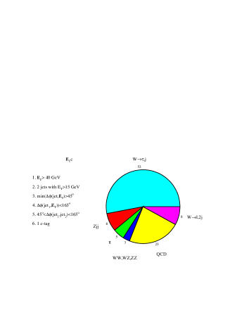
Figure 15: Selection cuts and composition of $\hbox to0.0pt{\hbox to7.95831pt{\hfil/\hfil}\hss}E_{T}c$ sample.

More than 50% of the background is composed of $W(\to\tau\nu)+1$ jet events.

$W+c$ production

The leading order production process for $W(\to\tau\nu)+1$ jet, where this jet is identified as charm, is $sg\to Wc$. The main uncertainty of the production rate for this process comes from the PDF of sea $s$ quarks $f_{s}(x)$, which is measured by NuTeV [80] in the neutrino scattering process $\nu_{\mu}s\to\mu c$.

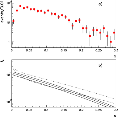
Figure 16: (a) Distribution in $x$ of sea $s$-quarks that contribute to $sg\to Wc$ production at the Tevatron, generated with PYTHIA 6.1+CTEQ4LO. Selection cuts have been applied. (b) Solid lines represent $f_{s}(x)$ and its uncertainty, as measured by NuTeV. It is compared to GRV94LO (dashed line) and CTEQ4LO (dot-dashed line) strange sea distributions.

Figure 16 (a) shows the distribution in $x$ of sea $s$-quarks that contribute to $sg\to Wc$ production at the Tevatron after the selection cuts from Figure 15 have been applied. Figure 16 (b) shows the $f_{s}(x)$ and its uncertainty measured by NuTeV. As we see, the region of NuTeV sensitivity is relevant for Tevatron studies. The overall uncertainty on $f_{s}(x)$ is 13.5%. $f_{s}(x)$ measured by NuTeV is in a good agreement with the results of CCFR [81], which has an uncertainty of 10.5%.

Since these uncertainties are dominated by the experimental statistics, we can hope that the combined result will have an uncertainty near 8.5%. The strange sea parton density function was also measured by the CHARM II [82] and CDHS [83] experiments. Combination of results of all four experiments is certainly desirable, but non–trivial, since somewhat different techniques where used in each analysis.

In Figure 16(b), $f_{s}(x)$ measured by NuTeV is compared to the one provided by the GRV94LO [84] and CTEQ4LO [85] PDF’s, which are shown by dashed and dot-dashed lines, respectively. None of the PDF’s provide an adequate description of the strange sea data. In the Tevatron search experiments, the systematic uncertainty on the background due to PDF’s was typically estimated by switching from one PDF to another. In this case, the systematic uncertainty on the number of $Wc$ events that pass our cuts is 36%. If instead of CTEQ4LO, $f_{s}(x)$ measured by NuTeV were used, the number of expected $Wc$ events would go down by 30%. This is within the estimated uncertainty, but clearly the uncertainty has been overestimated. The correct uncertainty to use is 13.5%, or 8.5%, when the results of NuTeV and CCFR will be combined. This is a significant reduction compared to 36%, yet it is still not down to the desirable level of 5%. We can probably do better by studying $Wc$ production when the $W$ is identified by its decay to a muon or an electron. The expected number of events in the $Wc,W\to\ell\nu(\ell=e,\mu)$ channel is about 2800, after applying the cuts listed in Figure 15, which corresponds to the statistical uncertainty for this background of about 2%. The systematic uncertainty on missing energy and charm identification are common to the two channels, and the difference is in lepton vs. tau identification uncertainty, which can be expected to be below 5% with Run II statistics.

QCD background

The next dominant background in the $\hbox to0.0pt{\hbox to7.95831pt{\hfil/\hfil}\hss}E_{T}c$ channel is QCD multijet production, where missing energy comes from jet energy mis-measurement. This background is the toughest one to estimate, because it involves multiple gluon radiation and splitting. Not only the overall rate, but also the angular correlation between jets may not be predicted reliably. To isolate this component, the usual trick is to apply all the signal selection cuts except tagging, subtract other known backgrounds and call the rest “QCD.” The tagging probability derived from an independent jet sample is then applied to estimate the QCD contribution to the tagged sample [86]. One obvious drawback is that the heavy flavor fraction can change after the cuts are applied. Another is that the signal contribution is not always negligible even before tagging, and to some extent, it may be normalized away.

Other backgrounds in the $\hbox to0.0pt{\hbox to7.95831pt{\hfil/\hfil}\hss}E_{T}c$ channel.

Other backgrounds in the $\hbox to0.0pt{\hbox to7.95831pt{\hfil/\hfil}\hss}E_{T}c$ channel are top pair production, di-bosons, $Z+$ jets and $W+$ jets, where leptons were not identified. The discussion of these processes in Section 6.3 applies to the $\hbox to0.0pt{\hbox to7.95831pt{\hfil/\hfil}\hss}E_{T}c$ channel as well.

7 Variable flavor number schemes for heavy quark electroproduction

by J. Smith

Heavy quark production has been a major topic of investigation at hadron-hadron, electron-proton and electron-positron colliders. Here a review is given of some topics which are of interest primarily for electron-proton colliders. We concentrate on this reaction because a theoretical treatment can be based on the operator product expansion, and also because data are available for deep-inelastic charm production at HERA. How all this relates to Fermilab experiments will be discussed at the end.

In QCD perturbation theory, one needs to introduce a renormalization scale and a mass factorization scale to perform calculations. We choose both equal to $\mu^{2}$, which will be a function of $Q^{2}$ and the square of the mass of the charm quark $m^{2}$. At small $\mu^{2}$, where kinematic effects due to quark masses are important, the best way to describe charm quark production is via heavy quark pair production from light quark $u,d,s$ and gluon initial states. The mass $m$ only appears in the heavy quark coefficient functions (or partonic cross sections) like $H_{i,g}^{\rm S,(2)}(z,Q^{2},m^{2},\mu^{2})$, etc., [87]. Here the superscripts refer to their flavor decomposition and the order in perturbation theory, while the subscripts refer to the projection $i=2,L$ and the partonic initial state. The arguments refer to the partonic Bjorken variable $z=Q^{2}/(s+Q^{2})$ and to the fact that these functions depend upon invariants and scales. The renormalization necessary to calculate these NLO expressions follows the CWZ method [88]. The symbol $H$ refers to those coefficient functions which are derived from Feynman diagrams where the virtual photon couples to a heavy quark line. Analytic expressions for these functions are not known, but numerical fits are available in [89]. Asymptotic expressions in the limit $Q^{2}\gg m^{2}$ are available in [90]. These contain terms like $\ln^{2}(Q^{2}/m^{2})$ and $\ln(Q^{2}/m^{2})\ln(Q^{2}/\mu^{2})$ multiplied by functions of $z$; they are manifestly singular in the limit that $m\rightarrow 0$.

There are other heavy quark coefficient functions such as $L_{i,q}^{\rm NS,(2)}(z,Q^{2},m^{2})$, which arise from tree diagrams where the virtual photon attaches to the an initial state light quark line, so the heavy-quark is pair produced via virtual gluons. Analytic expressions for these functions are known for all $z$, $Q^{2}$ and $m^{2}$, which, in the limit $Q^{2}\gg m^{2}$ contain powers of $\ln(Q^{2}/m^{2})$ multiplied by functions of $z$. The three-flavor light mass $\overline{\rm MS}$ parton densities can be defined in terms of matrix elements of operators and are now available in parton density sets. This is a fixed order perturbation theory (FOPT) description of heavy quark production with three-flavor parton densities. Due to the work in [87], the perturbation series is now known up to second order. In regions of moderate scales and invariants, this NLO description is well defined and can be combined with a fragmentation function to predict exclusive distributions [91] for the outgoing charm meson, the anti-charm meson and the additional parton. This NLO massive charm approach agrees well with the recent $D$-meson inclusive data in [92] and [93]. The charm quark structure functions in this NLO description will be denoted $F^{\rm EXACT}_{i,c}(x,Q^{2},m^{2},n_{f}=3)$.

A different description, which should be more appropriate for large scales where terms in $m^{2}$ are negligible, is to represent charm production by a parton density $f_{c}(x,\mu^{2})$, with a boundary condition that the density vanishes at small values of $\mu^{2}$. Although at first sight these approaches appear to be completely different, they are in fact intimately related. It was shown in [94] that the large terms in $\ln(Q^{2}/m^{2})$ which arise when $Q^{2}\gg m^{2}$, can be resummed to all orders in perturbation theory. In this reference, all the two-loop corrections to the matrix elements of massive quark and massless gluon operators in the operator product expansion were calculated. These contain the same type of logarithms mentioned above multiplied by functions of $z$ (which is the last Feynman integration parameter). After operator renormalization and suitable reorganization of convolutions of the operator matrix elements (OME’s) and the coefficient functions, the expressions for the infrared-safe charm quark structure functions $F_{i,c}(x,Q^{2},m^{2},\Delta)$ take on a simple form. After resummation, they are convolutions of light-mass, four-flavor parton coefficient functions, commonly denoted by expressions like ${\cal C}^{\rm S,(2)}_{i,g}(Q^{2}/\mu^{2})$ (available in [95], [96]), with four-flavor light-parton densities, which also include a charm quark density $f_{c}(x,\mu^{2})$. Since the corrections to the OME’s contain terms in $\ln(Q^{2}/m^{2})$ and $\ln(m^{2}/\mu^{2})$ as well as non-logarithmic terms, it is simplest to work in the $\overline{\rm MS}$ scheme with the scale $\mu^{2}=m^{2}$ for $Q^{2}\leq m^{2}$ and $\mu^{2}=m^{2}+Q^{2}(1-m^{2}/Q^{2})^{2}/2$ for $Q^{2}>m^{2}$ and discontinuous matching conditions on the flavor densities at $\mu^{2}=m^{2}$. Then all the logarithmic terms vanish at $Q^{2}=\mu^{2}=m^{2}$ and the non-logarithmic terms in the OME’s are absorbed into the boundary conditions on the charm density, the new four-flavor gluon density and the new light-flavor u,d,s densities. The latter are convolutions of the previous three-flavor densities with the OME’s given in the Appendix of [94].

The above considerations lead to a precise description through order $\alpha_{s}^{2}$ of how, in the limit $m\rightarrow 0$, to re-express the $F_{i,c}^{\rm EXACT}(x,Q^{2},m^{2})$ written in terms of convolutions of heavy quark coefficient functions with three-flavor light parton densities into a description in terms of four-flavor light-mass parton coefficient functions convoluted with four-flavor parton densities. This procedure leads to the so-called zero-mass variable-flavor-number scheme (ZM-VFNS) for $F_{i,c}(x,Q^{2},\Delta)$ where the $m$ dependent logarithms are absorbed into the new four-flavor densities. To implement this scheme, one has to be careful to use inclusive quantities which are collinearly finite in the limit $m\rightarrow 0$ and $\Delta$ is an appropriate parameter which enables us to do this. In the expression for $F_{i,c}$ there is a cancellation of terms in $\ln^{3}(Q^{2}/m^{2})$ between the two-loop corrections to the light quark vertex function (the Sudakov form factor) and the convolution of the densities with the soft part of the $L_{2,q}$-coefficient function. This is the reason for the split of $L_{i,q}$ into soft and hard parts, via the introduction of a constant $\Delta$. Details and analytic results for $L_{i,c}^{\rm SOFT}$ and $L_{i,c}^{\rm HARD}$ are available in [97]. All this analysis yielded and used the two-loop matching conditions on variable-flavor parton densities across flavor thresholds, which are special scales where one makes transitions from say a three-flavor massless parton scheme to a four-flavor massless parton scheme. The threshold is a choice of $\mu$ which has nothing to do with the actual kinematical heavy flavor pair production threshold at $Q^{2}(x^{-1}-1)=4m^{2}$. In [94],[98] it was shown that the $F^{\rm EXACT}_{i,c}(x,Q^{2},m^{2},n_{f}=3)$ tend numerically to the known asymptotic results in $F^{\rm ASYMP}_{i,c}(x,Q^{2},m^{2},n_{f}=3)$, when $Q^{2}\gg m^{2}$, which also equal the ZM-VFNS results. The last description is good for large (asymptotic) scales and contains a charm density $f_{c}(x,\mu^{2})$ which satisfies a specific boundary condition at $\mu^{2}=m^{2}$. We denote the charm quark structure functions in this description by $F^{\rm PDF}_{i,c}(x,Q^{2},n_{f}=4)$.

For moderate values of $Q^{2}$, a third approach has been introduced to describe the charm components of $F_{i}(x,Q^{2})$. This is called a variable flavor number scheme (VFNS). A first discussion was given in [99], where a VFNS prescription called ACOT was given in lowest order only. A proof of factorization to all orders was recently given in [100] for the total structure functions $F_{i}(x,Q^{2})$, but the NLO expressions for $F_{i,c}(x,Q^{2},m^{2})$ in this scheme were not provided. An NLO version of a VFNS scheme has been introduced in [97] and will be called the CSN scheme. A different approach, also generalized to all orders, was given in [94],[98], which is called the BMSN scheme. Finally another version of a VFNS was presented in [101], which is called the TR scheme. The differences between the various schemes can be attributed to two ingredients entering the construction of a VFNS. The first one is the mass factorization procedure carried out before the large logarithms can be resummed. The second one is the matching condition imposed on the charm quark density, which has to vanish in the threshold region of the production process. All VFNS approaches require two sets of parton densities. One set contains three-flavor number densities whereas the second set contains four-flavor number densities. The sets have to satisfy the $\overline{\rm MS}$ matching relations derived in [94]. Appropriate four-flavor densities have been constructed in [97] starting from the three-flavor LO and NLO sets of parton densities recently published in [102].

trick

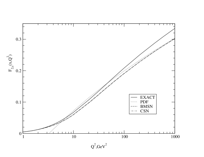
Figure 17: The charm quark structure functions $F_{2,c}^{\rm EXACT}(n_{f}=3)$ (solid line) $F_{2,c}^{\rm CSN}(n_{f}=4)$, (dot-dashed line) $F_{2,c}^{\rm BMSN}(n_{f}=4)$, (dashed line) and $F_{2,c}^{\rm PDF}(n_{f}=4)$, (dotted line) in NNLO for $x=0.005$ plotted as functions of $Q^{2}$.

Since the formulae for the heavy quark structure functions are available in [97], we only mention a few points here. The BMSN scheme avoids the introduction of any new coefficient functions other than those above. Since the asymptotic limits for $Q^{2}\gg m^{2}$ of all the operator matrix elements and coefficient functions are known, we define (here $Q$ refers to the heavy charm quark)

$$F_{i,Q}^{\rm BMSN}(x,Q^{2},m^{2},\Delta,n_{f}=4)=\\[2.84526pt] F_{i,Q}^{\rm EXACT}(x,Q^{2},m^{2},\Delta,n_{f}=3)\\[8.61108pt] -F_{i,Q}^{\rm ASYMP}(x,Q^{2},m^{2},\Delta,n_{f}=3)\\[2.84526pt] +F_{i,Q}^{\rm PDF}(x,Q^{2},m^{2},\Delta,n_{f}=4)\,.$$ (33)

The scheme for $F_{i,Q}^{\rm CSN}$ introduces a new heavy quark OME $A_{QQ}^{\rm NS,(1)}(z,\mu^{2}/m^{2})$ [103] and coefficient functions $H_{i,Q}^{\rm NS,(1)}(z,Q^{2}/m^{2})$ [104] because it requires an incoming heavy quark $Q$, which did not appear in the NLO corrections in [87]. The CSN coefficient functions are defined via the following equations. Up to second order we have

$${\cal C}_{i,q,Q}^{\rm CSN,SOFT,NS,(2)}\Big{(}\Delta,\frac{Q^{2}}{m^{2}},\frac{Q^{2}}{\mu^{2}}\Big{)}=A_{qq,Q}^{\rm NS,(2)}\Big{(}\frac{\mu^{2}}{m^{2}}\Big{)}{\cal C}_{i,q}^{\rm NS,(0)}\\[2.84526pt] -\beta_{0,Q}\ln\left(\frac{\mu^{2}}{m^{2}}\right)\times{\cal C}_{i,q}^{\rm NS,(1)}\Big{(}\frac{Q^{2}}{\mu^{2}}\Big{)}-{\cal C}_{i,q}^{\rm VIRT,NS,(2)}(\frac{Q^{2}}{m^{2}})\\[2.84526pt] -L_{i,q}^{\rm SOFT,NS,(2)}\Big{(}\Delta,\frac{Q^{2}}{m^{2}},\frac{Q^{2}}{\mu^{2}}\Big{)}\,,$$ (34)

with the virtual term the second order Sudakov form factor.

trick

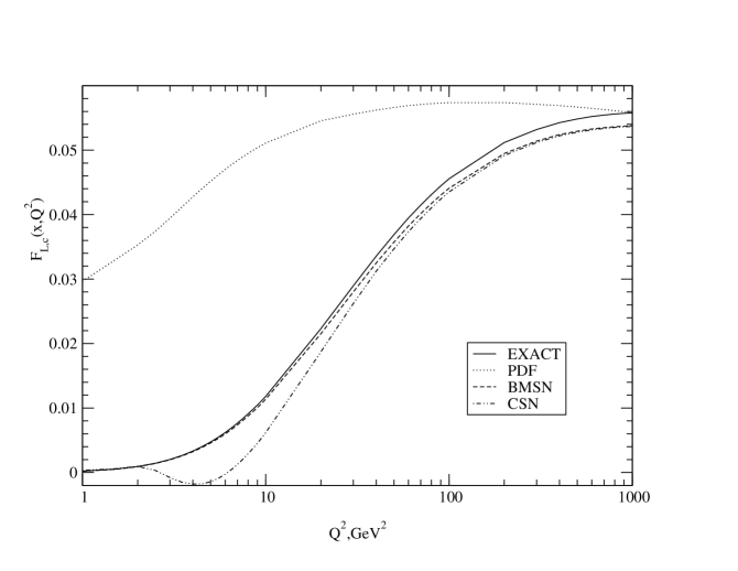
Figure 18: The charm quark structure functions $F_{L,c}^{\rm EXACT}(n_{f}=3)$ (solid line) $F_{L,c}^{\rm CSN}(n_{f}=4)$, (dot-dashed line) $F_{L,c}^{\rm BMSN}(n_{f}=4)$, (dashed line) and $F_{L,c}^{\rm PDF}(n_{f}=4)$, (dotted line) in NNLO for $x=0.005$ plotted as functions of $Q^{2}$.

The other CSN coefficient functions are defined by equations like (we only give one of the longitudinal terms for illustration)

$${\cal C}_{L,g}^{\rm CSN,S,(1)}\Big{(}\frac{Q^{2}}{m^{2}},\frac{Q^{2}}{\mu^{2}}\Big{)}=\\[2.84526pt] H_{L,g}^{\rm S,(1)}\Big{(}\frac{Q^{2}}{m^{2}}\Big{)}-A_{Qg}^{\rm S,(1)}(\frac{\mu^{2}}{m^{2}})\,{\cal C}_{L,Q}^{\rm CSN,NS,(0)}\Big{(}\frac{Q^{2}}{m^{2}}\Big{)}\,,$$ (35)

with ${\cal C}_{L,Q}^{\rm CSN,NS,(0)}={4m^{2}}/{Q^{2}}$. The CSN and BMSN schemes are designed to have the following two properties. First of all, suppressing unimportant labels,

$$F_{i,Q}^{\rm CSN}(n_{f}=4)=F_{i,Q}^{\rm BMSN}(n_{f}=4)\\[2.84526pt] =F_{i,Q}^{\rm EXACT}(n_{f}=3)\quad\mbox{for}\quad Q^{2}\leq m^{2}\,.$$ (36)

Since $f_{Q}(m^{2})^{\rm NNLO}\not=0$ (see [94]) this condition can be only satisfied when we truncate the perturbation series at the same order. The second requirement is that

$$\mathop{\mbox{lim}}\limits_{\vphantom{\frac{A}{A}}Q^{2}\gg m^{2}}F_{i,Q}^{\rm BMSN}(n_{f}=4)=\mathop{\mbox{lim}}\limits_{\vphantom{\frac{A}{A}}Q^{2}\gg m^{2}}F_{i,Q}^{\rm CSN}(n_{f}=4)\\[2.84526pt] =\mathop{\mbox{lim}}\limits_{\vphantom{\frac{A}{A}}Q^{2}\gg m^{2}}F_{i,Q}^{\rm PDF}(n_{f}=4)\,.$$ (37)

The only differences between the two schemes arises from terms in $m^{2}$ so they may not be equal just above $Q^{2}=m^{2}$. This turns out to be the case for the longitudinal structure function, which is more sensitive to mass effects.

Figure 17 shows NNLO results for the $Q^{2}$ dependence of $F_{2,c}^{\rm EXACT}(n_{f}=3)$, $F_{2,c}^{\rm CSN}(n_{f}=4)$, $F_{2,c}^{\rm BMSN}(n_{f}=4)$, and $F_{2,c}^{\rm PDF}(n_{f}=4)$ at $x=0.005$. Note that the results satisfy the requirements in Eqs. (36) and (37). The ZM-VFNS description is poor at small $Q^{2}$. Figure 18 shows the results for $F_{L,c}^{\rm EXACT}(n_{f}=3)$, $F_{L,c}^{\rm CSN}(n_{f}=4)$, $F_{L,c}^{\rm BMSN}(n_{f}=4)$, and $F_{L,c}^{\rm PDF}(n_{f}=4)$ at $x=0.005$. We see that the CSN result is negative and therefore unphysical for $2.5<Q^{2}<6$ $({\rm GeV}/c)^{2}$ which is due to the term in $4m^{2}/Q^{2}$ and the subtraction in Eq. (35).

One way this research work is of relevance to Fermilab experiments is that it produces more precise ZM-VFNS parton densities. Such densities are used extensively to predict cross sections at high energies, for example for single top quarks. Therefore the previous work on four-flavor parton densities has been extended in [105] to incorporate the two-loop discontinuous matching conditions across the bottom flavor threshold at $\mu=m_{b}$ and provided a set of five-flavor densities, which contains a bottom quark density $f_{b}(x,\mu^{2})$. The differences between the five-flavor densities and those in [106] and [35] are also discussed. Results for deep-inelastic electroproduction of bottom quarks will be presented in [107].

8 The Underlying Event in Hard Scattering Processes

by Rick Field and David Stuart

8.1 Introduction

The total proton-antiproton cross section is the sum of the elastic and inelastic cross sections. The inelastic cross section consists of a single-diffractive, double-diffractive, and a “hard core” component, where the “hard core” is everything else. “Hard core” does not necessarily imply “hard scattering.” A “hard scattering” collision, such as that illustrated in Fig. 19(a), is one in which a “hard” (i.e. large transverse momentum) 2-to-2 parton-parton subprocess has occurred. “Soft” hard core collisions correspond to events in which no “hard” interaction has occurred. When there is no large $p_{T}$ subprocess in the collision, one is not probing short distances and it probably does not make any sense to talk about partons. The QCD “hard scattering” cross section grows with increasing collider energy and becomes a larger and larger fraction of the total inelastic cross section. In this analysis, we used the CDF Min-Bias trigger data sample in conjunction with the JET20 trigger data sample to study the growth and development of “charged particle jets” from $p_{T}({\rm jet})=0.5$ to $50{\rm\,GeV}$. We compared several “local” jet observables with the QCD “hard scattering” Monte-Carlo models of HERWIG[1], ISAJET[2], and PYTHIA[3].

         

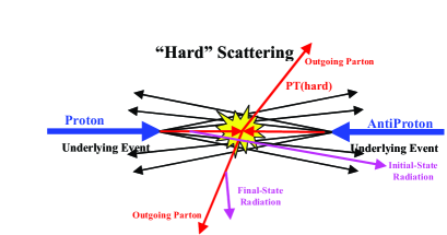
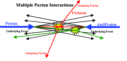
Figure 19: (a) Illustration of a $p\bar{p}$ collision in which a “hard” 2-to-2 parton scattering with transverse momentum, $p_{T}({\rm hard})$, has occurred. The resulting event contains particles that originate from the two outgoing partons (plus final-state radiation) and particles that come from the breakup of the $p$ and $\bar{p}$ (i.e., “beam-beam remnants”). The “underlying event” consists of the beam-beam remnants plus initial-state radiation; (b) Illustration of a $p\bar{p}$ collision in which a multiple parton interaction has occurred. In addition to the “hard” 2-to-2 parton scattering with transverse momentum, $p_{T}({\rm hard})$, there is an additional “semi-hard” parton-parton scattering that contributes particles to the “underlying event.” For PYTHIA, we include the contributions from multiple parton scattering in the beam-beam remnant component.

A “hard scattering” event, like that illustrated in Fig. 19(a) consists of large-$p_{T}$ outgoing hadrons that originate from the large-$p_{T}$ partons (i.e., outgoing hard scattering “jets”) and also hadrons that originate from the break-up of the proton and antiproton (i.e., the “beam-beam remnants”). The “underlying event” is an interesting object that is not very well understood. In addition to beam-beam remnants, it may contain hadrons resulting from initial-state radiation. Also, it is possible that multiple parton scattering occurs in hadron-hadron collisions as illustrated in Fig. 19(b). This is a controversial issue, but the underlying event might also contains hadrons that originate from multiple parton interactions. PYTHIA, for example, uses multiple parton interactions as a way to enhance the activity of the underlying event [3].

In this analysis, we studied a variety of “global” observables to probe the growth and structure of the underlying event. We find that the underlying “hard scattering” event is not the same as a “soft” $p\bar{p}$ collision. For the same available energy, the underlying event in a hard scattering is considerably more active (i.e., higher charged particle density and more $p_{T}$) than a “soft” collision. This is not surprising since a violent hard scattering has occurred! We find that none of the QCD Monte-Carlo models (with their default parameters) describe correctly all the properties of the underlying event.

8.2 Data Selection and Monte-Carlo Models

(1) Data Selection

The CDF detector, described in detail in Ref. [122], measures the trajectories and transverse momenta, $p_{T}$, of charged particles in the pseudorapidity region $|\eta|<1.1$ with the central tracking chamber (CTC), silicon vertex detector (SVX), and vertex time projection chamber (VTX), which are immersed in a $1.4$ T solenoidal magnetic field. In this analysis we consider only charged particles measured in the central tracking chamber (CTC) and use the two trigger sets of data listed in Table 9. The minimum bias (min-bias) data were selected by requiring that at least one particle interacted with the forward beam-beam counter BBC ($3.4<\eta<5.9$) and/or the backward BBC ($-5.9<\eta<-3.4$). The min-bias trigger selects predominately the “hard core” component of the inelastic cross section.

Charged particle tracks are found with high efficiency as long as the density of particles is not high. To remain in a region of high efficiency, we consider only charged particles with $p_{T}>0.5{\rm\,GeV}$ and $|\eta|<1$. The observed tracks include some fake tracks that result from secondary interactions between primary particles, including neutral particles, and the detector material. There are also particles originating from other $p\bar{p}$ collisions. To reduce the contribution from these sources, we consider only tracks which point to the primary interaction vertex within $2$ cm along the beam direction and $1$ cm transverse to the beam direction. Detector simulations indicate that this impact parameter cut is very efficient and that the number of fake tracks is about $3.5\%$ when a $1$ cm impact parameter cut is applied in conjunction with a $2$ cm vertex cut. Without the impact parameter cut the number of fake tracks is approximately $9\%$.

This dependence of the number of fake tracks on the CTC impact parameter cut provides a method of estimating systematic uncertainties due to fakes. Every data point $P$ on every plot in this analysis was determined three times by using a $2$ cm vertex cut in conjunction with three different CTC $d_{0}$ cuts; a $1$ cm CTC $d_{0}$ cut ($P$), a $0.5$ cm CTC $d_{0}$ cut ($P_{1}$), and no CTC $d_{0}$ cut ($P_{2}$). The $1$ cm cut determined the value of the data point, $P$, and the difference between the $0.5$ cm cut value and no cut value of the data point determined the systematic error of the data point as follows: sys-error $=P|P_{2}-P_{1}|/P_{1}$ This systematic error was then added in quadrature with the statistical error. We do not correct the data for the CTC track-finding efficiency. Instead, the theoretical Monte-Carlo model predictions are corrected.

Table 9: Data sets and selection criterion used in this analysis.

CDF Data Set	Trigger	Events	Selection
Min-Bias	Min-Bias Trigger	626,966	zero or one vertex in $|z|<100$ cm
			$|z_{c}-z_{v}|<2$ cm, $|{\rm CTC}\ d_{0}|<1$ cm
			$p_{T}^{\rm track}>0.5{\rm\,GeV}$, $|\eta|<1$
JET20	Calorimeter Tower cluster	78,682	zero or one vertex in $|z|<100$ cm
	with $E_{T}>20{\rm\,GeV}$		$|z_{c}-z_{v}|<2$ cm, $|{\rm CTC}\ d_{0}|<1$ cm
			$p_{T}^{\rm track}>0.5{\rm\,GeV}$, $|\eta|<1$

(2) QCD “Hard Scattering” Monte-Carlo Models

The “hard” scattering QCD Monte-Carlo models used in this analysis are listed in Table 10. The QCD perturbative 2-to-2 parton-parton differential cross section diverges as the $p_{T}$ of the scattering, $p_{T}^{\rm hard}$, goes to zero (see Fig. 19). One must set a minimum $p_{T}^{\rm hard}$ large enough so that the resulting cross section is not larger that the total “hard core” inelastic cross section, and also large enough to ensure that QCD perturbation theory is applicable. In this analysis we take $p_{T}^{\rm hard}>3{\rm\,GeV}$.

Table 10: Theoretical QCD “hard” scattering Monte-Carlo models studied in this analysis. In all cases we take $p_{T}({\rm hard})>3{\rm\,GeV}$.

Monte-Carlo Model	Subprocess	Comments
HERWIG 5.9	QCD 2-to-2 parton scattering	Default values for all parameters
	IPROC = 1500
ISAJET 7.32	QCD 2-to-2 parton scattering	Default values for all parameters
	TWOJET
PYTHIA 6.115	QCD 2-to-2 parton scattering	Default values for all parameters:
	MSEL = 1	PARP(81) = $1.4$
PYTHIA 6.125	QCD 2-to-2 parton scattering	Default values for all parameters:
	MSEL = 1	PARP(81) = $1.9$
PYTHIA No MS	QCD 2-to-2 parton scattering	Default values for all parameters:
	MSEL = 1	MSTP(81) = $0$

Each of the QCD Monte-Carlo models handle the “beam-beam remnants” in a similar fashion. A hard scattering event is basically the superposition of a hard parton-parton interaction on top of a “soft” collision. HERWIG[1] assumes that the underlying event is a soft collision between the two “beam clusters.” ISAJET[2] uses a model similar to the one it uses for soft “min-bias” events (i.e., “cut Pomeron”), but with different parameters, to describe the underlying beam-beam remnants. PYTHIA[3] assumes that each incoming beam hadron leaves behind a “beam remnant,” which do not radiate initial state radiation, and simply sail through unaffected by the hard process. However, unlike HERWIG and ISAJET, PYTHIA also uses multiple parton interactions to enhance the activity of the underlying event as illustrated in Fig. 19.

In this analysis we examine two versions of PYTHIA, PYTHIA 6.115 and PYTHIA 6.125 both with the default values for all the parameters. The default values of the parameters are different in version 6.115 and 6.125. In particular, the effective minimum $p_{T}$ for multiple parton interactions, PARP(81), changed from $1.4{\rm\,GeV}$ in version 6.115 to $1.9{\rm\,GeV}$ in version 6.125. Increasing this cut-off decreases the multiple parton interaction cross section which reduces the amount of multiple parton scattering. For completeness, we also consider PYTHIA with no multiple parton scattering (MSTP(81)=0).

Since ISAJET employs “independent fragmentation” it is possible to trace particles back to their origin and divide them into three categories: particles that arise from the break-up of the beam and target (beam-beam remnants), particles that arise from initial-state radiation, and particles that result from the outgoing hard scattering jets plus final-state radiation. The “hard scattering component” consists of the particles that arise from the outgoing hard scattering jets plus initial and final-state radiation (sum of the last two categories). Particles from the first two categories (beam-beam remnants plus initial-state radiation) are normally what is referred to as the underlying event (see Fig. 19). Of course, these categories are not directly observable experimentally. Nevertheless, it is instructive to examine how particles from various origins affect the experimental observables.

Since HERWIG and PYTHIA do not use independent fragmentation, it is not possible to distinguish particles that arise from initial-state radiation from those that arise from final-state radiation, but we can identify the beam-beam remnants. When, for example, a color string breaks into hadrons it is not possible to say which of the two partons producing the string was the parent. For HERWIG and PYTHIA, we divide particles into two categories: particles that arise from the break-up of the beam and target (beam-beam remnants), and particles that result from the outgoing hard scattering jets plus initial and final-state radiation (hard scattering component). For PYTHIA, we include particles that arise from multiple parton interactions in the beam-beam remnant component.

(3) Method of Comparing Theory with Data

Our philosophy in comparing the theory with data in this analysis is to select a region where the data is very “clean.” The CTC efficiency can vary substantially for very low $p_{T}$ tracks and in dense high $p_{T}$ jets. To avoid this we have considered only the region $p_{T}>0.5{\rm\,GeV}$ and $|\eta|<1$ where the CTC efficiency is high and stable (estimated to be $92\%$ efficient) and we restrict ourselves to jets less than $50{\rm\,GeV}$. The data presented here are uncorrected. Instead the theoretical Monte-Carlo predictions are corrected for the track finding efficiency and have an error (statistical plus systematic) of about $5\%$. The errors on the (uncorrected) data include both statistical and correlated systematic uncertainties.

In comparing the QCD “hard scattering” Monte-Carlo models with the data, we require that the Monte-Carlo events satisfy the CDF min-bias trigger and we apply an $8\%$ correction for the CTC track finding efficiency. The corrections are small. On the average, $8$ out of every $100$ charged particles predicted by the theory are removed from consideration. Requiring the theory to satisfy the min-bias trigger is important when comparing with the Min- Bias data, but does not matter when comparing with the JET20 data since essentially all high $p_{T}$ jet events satisfy the min-bias trigger.

8.3 The Evolution of Charge Particle “Jets” from $0.5$ to $50$ GeV

We define charged particle “jets” and examine the evolution of these “jets” from $p_{T}^{\rm jet}=0.5$ to $50{\rm\,GeV}$. As illustrated in Fig. 20, “jets” are defined as “circular regions” ($R=0.7$) in $\eta$-$\phi$ space and contain charged particles from the underlying event as well as particles which originate from the fragmentation of high $p_{T}$ outgoing partons (see Fig. 19). Also, every charged particle in the event is assigned to a “jet,” with the possibility that some “jets” might consist of just one charged particle. We adapt a very simple jet definition since we will be dealing with “jets” that consist of only a few low $p_{T}$ charged particles. The standard jet algorithm based on calorimeter clustering is not applicable at low $p_{T}$.

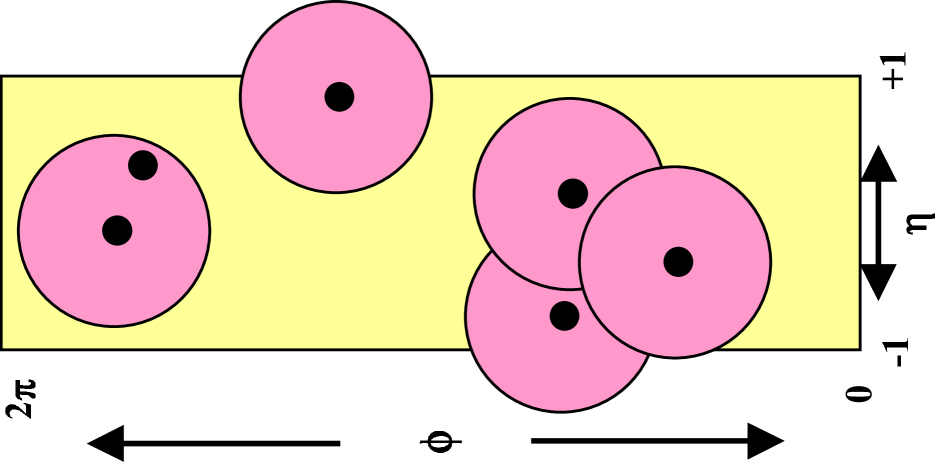
Figure 20: Illustration of an event with six charged particles ($p_{T}>0.5{\rm\,GeV}$ and $|\eta|<1$) and five charged “jets” (circular regions in $\eta$-$\phi$ space with $R=0.7$).

(1) Jet Definition (charged particles)

We define jets as circular regions in $\eta$-$\phi$ space with “distance” $R=\sqrt{(\Delta\eta)^{2}+(\Delta\phi)^{2}}$. Our jet algorithm is as follows:

• Order all charged particles according to their $p_{T}$.

• Start with the highest $p_{T}$ particle and include in the “jet” all particles within $R=0.7$.

• Go to the next highest $p_{T}$ particle (not already included in a “jet”) and add to the “jet” all particles (not already included in a “jet”) within $R=0.7$.

• Continue until all particles are in a “jet.”

We consider all charged particles ($p_{T}>0.5{\rm\,GeV}$ and $|\eta|<1$) and allow the jet radius to extend outside $|\eta|<1$. Fig. 20 illustrates an event with six charged particles and five jets. We define the $p_{T}$ of the jet to be the scalar $p_{T}$ sum of all the particles within the jet (i.e., it is simply the scalar $p_{T}$ sum within the circular region).

We know that the simple charged particle jet definition used here is not theoretically favored since if applied at the parton level it is not infrared safe. Of course, all jet definitions (and in fact all observables) are infrared safe at the hadron level. We have done a detailed study comparing the na ve jet definition used here with a variety of more sophisticated charge particle jet definitions. This analysis will be presented in a future publication. Some of the observables presented here do, of course, depend on one’s definition of a jet and it is important to apply the same definition to both the theory and data.

(2) Charged Jet Multiplicity versus $p_{T}({\rm jet\#1})$

Fig. 21 shows the average number of charged particles ($p_{T}>0.5{\rm\,GeV}$ and $|\eta|<1$) within jet#1 (leading charged jet) as a function of $p_{T}({\rm jet\#1})$. The solid points are Min-Bias data and the open points are the JET20 data. The JET20 data connect smoothly to the Min-Bias data and allow us to study observables over the range $0.5<p_{T}({\rm jet\#1})<50{\rm\,GeV}$. There is a small overlap region where the Min-Bias and JET20 data coincide. The errors on the data include both statistical and correlated systematic uncertainties, however, the data have not been corrected for efficiency. Fig. 21 shows a sharp rise in the leading charged jet multiplicity at low $p_{T}({\rm jet\#1})$ and then a flattening out and a gradual rise at high $p_{T}({\rm jet\#1})$. The data are compared with the QCD “hard scattering” Monte-Carlo predictions of HERWIG 5.9, ISAJET 7.32, and PYTHIA 6.115. The theory curves are corrected for the track finding efficiency and have an error (statistical plus systematic) of around $5\%$.

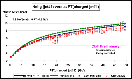
Figure 21: The average number of charged particles ($p_{T}>0.5{\rm\,GeV}$ and $|\eta|<1$) within the leading charged jet ($R=0.7$) as a function of the $p_{T}$ of the leading charged jet. The solid (open) points are Min-Bias (JET20) data. The errors on the (uncorrected) data include both statistical and correlated systematic uncertainties. The QCD “hard scattering” theory curves (HERWIG 5.9, ISAJET 7.32, PYTHIA 6.115) are corrected for the track finding efficiency and have an error (statistical plus systematic) of around $5\%$.

(3) Charged Jet “Size” versus $p_{T}({\rm jet\#1})$

Although the charged particle jets are defined as circular regions in $\eta$-$\phi$ space with $R=0.7$, this is not the “size” of the jet. The “size” of a jet can be defined in two ways: size according to particle number and size according to $p_{T}$. The first corresponds to the radius in $\eta$-$\phi$ space that contains $80\%$ of the charged particles in the jet, and the second corresponds to the radius in $\eta$-$\phi$ space that contains $80\%$ of the jet $p_{T}$. The data on the average “jet size” of the leading charge particle jet are compared with the QCD “hard scattering” Monte-Carlo predictions of HERWIG 5.9, ISAJET 7.32, and PYTHIA 6.115 in Fig. 22. A leading $20{\rm\,GeV}$ charged jet has $80\%$ of its charged particles contained, on the average, within a radius in $\eta$-$\phi$ space of about $0.33$, and $80\%$ of its $p_{T}$ contained, on the average, within a radius of about $0.20$. Fig. 22 clearly illustrates the “hot core” of jets. The radius containing $80\%$ of the $p_{T}$ is smaller than the radius that contains $80\%$ of the particles. Furthermore, the radius containing $80\%$ of the $p_{T}$ decreases as the overall $p_{T}$ of the jet increases due to limited momentum perpendicular to the jet direction.

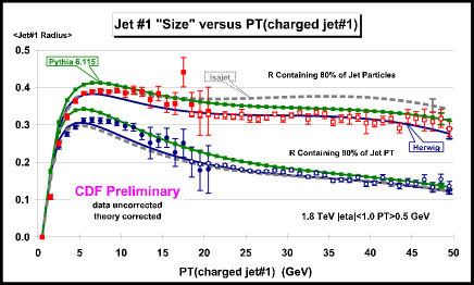
Figure 22: The average radius in $\eta$-$\phi$ space containing $80\%$ of the charged particles (and $80\%$ of the charged $p_{T}$) as a function of the $p_{T}$ of the leading charged jet. The errors on the (uncorrected) data include both statistical and correlated systematic uncertainties. The QCD “hard scattering” theory curves (HERWIG 5.9, ISAJET 7.32, PYTHIA 6.115) are corrected for the track finding efficiency and have an error (statistical plus systematic) of around $5\%$.

8.4 The Overall Event Structure as a Function of $p_{T}({\rm jet\#1})$

In the previous section, we studied “local” leading jets observables. The QCD Monte-Carlo models did not have to describe correctly the entire event in order to fit the observable. They only had to describe correctly the properties of the leading charge particle jet, and all the models fit the data fairly well (although not perfectly). Now we will study “global” observables, where to fit the observable the QCD Monte-Carlo models will have to describe correctly the entire event structure.

(1) Overall Charged Multiplicity versus $p_{T}({\rm jet\#1})$

Figure 23 shows the average number of charged particles in the event with $p_{T}>0.5{\rm\,GeV}$ and $|\eta|<1$ (including jet#1) as a function of $p_{T}({\rm jet\#1})$ (leading charged jet) for the Min-Bias and JET20 data. Again the JET20 data connect smoothly to the Min-Bias data, and there is a small overlap region where the Min-Bias and JET20 data coincide. Figure 23 shows a sharp rise in the overall charged multiplicity at low $p_{T}({\rm jet\#1})$ and then a flattening out and a gradual rise at high $p_{T}({\rm jet\#1})$ similar to Fig. 21. We would like to investigate where these charged particles are located relative to the direction of the leading charged particle jet.

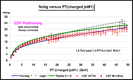
Figure 23: The average total number of charged particles in the event ($p_{T}>0.5{\rm\,GeV}$ and $|\eta|<1$ including jet#1) as a function of the $p_{T}$ of the leading charged jet. The solid (open) points are the Min- Bias (JET20) data. The errors on the (uncorrected) data include both statistical and correlated systematic uncertainties. The QCD “hard scattering” theory curves (HERWIG 5.9, ISAJET 7.32, PYTHIA 6.115) are corrected for the track finding efficiency and have an error (statistical plus systematic) of around $5\%$.

(2) Correlations in $\Delta\phi$ relative to $p_{T}({\rm jet\#1})$

As illustrated in Fig. 24, the angle $\Delta\phi$ is defined to be the relative azimuthal angle between charged particles and the direction of the leading charged particle jet. We label the region $|\phi-\phi_{\rm jet\#1}|<60^{\circ}$ as “toward” jet#1 and the region $|\phi-\phi_{\rm jet\#1}|>120^{\circ}$ is as “away” from jet#1. The “transverse” to jet#1 region is defined by $60^{\circ}<|\phi-\phi_{\rm jet\#1}|<120^{\circ}$. Each region, “toward,” “transverse,” and “away” covers the same range $|\Delta\eta|\times|\Delta\phi|=2\times 120^{\circ}$. The “toward” region includes the particles from jet#1 as well as a few particles from the underlying event. As we will see, the “transverse” region is very sensitive to the underlying event. The “away” region is a mixture of the underlying event and the “away-side” hard scattering jet.

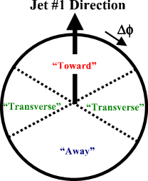
Figure 24: Illustration of correlations in azimuthal angle $\Delta\phi$ relative to the direction of the leading charged jet in the event, jet#1. The angle $\Delta\phi=\phi-\phi_{\rm jet\#1}$ is the relative azimuthal angle between charged particles and the direction of jet#1. The region $|\Delta\phi|<60^{\circ}$ is referred to as ”toward” jet#1 (includes particles in jet#1) and the region $|\Delta\phi|>120^{\circ}$ is called “away” from jet#1. The “transverse” to jet#1 region is defined by $60^{\circ}<|\Delta\phi|<120^{\circ}$. Each region, “toward,” “transverse,” and “away” covers the same range $|\Delta\eta|\times|\Delta\phi|=2\times 120^{\circ}$.

Figure 25 shows the data on the average number of charged particles ($p_{T}>0.5{\rm\,GeV}$ and $|\eta|<1$) as a function of $p_{T}({\rm jet\#1})$ for the three regions. Each point corresponds to the “toward,” “transverse,” or “away” $\langle N_{chg}\rangle$ in a $1{\rm\,GeV}$ bin. The solid points are Min-Bias data and the open points are JET20 data. The data in Fig. 25 define the average event “shape.” For example, for an “average” $p\bar{p}$ collider event at $1.8{\rm\,TeV}$ with $p_{T}({\rm jet\#1})=20{\rm\,GeV}$ there are, on the average, $8.7$ charged particles “toward” jet#1 (including the particles in jet#1), $2.5$ “transverse” to jet#1, and $4.9$ “away” from jet#1.

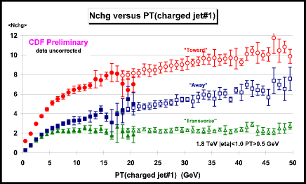
Figure 25: The average number of “toward” ($|\Delta\phi|<60^{\circ}$), “transverse” ($60^{\circ}<|\Delta\phi|<120^{\circ}$), and “away” ($|\Delta\phi|>120^{\circ}$) charged particles ($p_{T}>0.5{\rm\,GeV}$ and $|\eta|<1$ including jet#1) as a function of the $p_{T}$ of the leading charged jet. Each point corresponds to the $\langle N_{chg}\rangle$ in a $1{\rm\,GeV}$ bin. The solid (open) points are the Min-Bias (JET20) data. The errors on the (uncorrected) data include both statistical and correlated systematic uncertainties. The “toward,” “transverse,” and “away” regions are defined in Fig. 24.

Figure 26 shows the data on the average scalar $p_{T}$ sum of charged particles ($p_{T}>0.5{\rm\,GeV}$ and $|\eta|<1$) as a function of $p_{T}({\rm jet\#1})$ for the three regions. Here each point corresponds to the “toward,” “transverse,” or “away” $\langle{p_{T}}_{sum}\rangle$ in a $1{\rm\,GeV}$ bin. In Fig. 27, data on $\langle N_{chg}\rangle$ as a function of $p_{T}({\rm jet\#1})$ for the three regions are compared with the QCD “hard scattering” Monte-Carlo predictions of HERWIG 5.9, ISAJET 7.32, and PYTHIA 6.115. The QCD Monte-Carlo models agree qualitatively (but not precisely) with the data. We will now examine more closely these three regions.

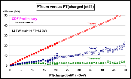
Figure 26: The average scalar $p_{T}$ sum of “toward” ($|\Delta\phi|<60^{\circ}$), “transverse” ($60^{\circ}<|\Delta\phi|<120^{\circ}$), and “away” ($|\Delta\phi|>120^{\circ}$) charged particles ($p_{T}>0.5{\rm\,GeV}$ and $|\eta|<1$ including jet#1) as a function of the $p_{T}$ of the leading charged jet. Each point corresponds to the $\langle PT_{sum}\rangle$ in a $1{\rm\,GeV}$ bin. The solid (open) points are the Min-Bias (JET20) data. The errors on the (uncorrected) data include both statistical and correlated systematic uncertainties. The “toward,” “transverse,” and “away” regions are defined in Fig. 24.

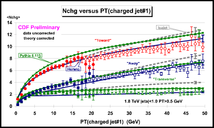
Figure 27: Data from Fig. 25 on the average number of “toward” ($|\Delta\phi|<60^{\circ}$), “transverse” ($60^{\circ}<|\Delta\phi|<120^{\circ}$), and “away” ($|\Delta\phi|>120^{\circ}$) charged particles ($p_{T}>0.5{\rm\,GeV}$ and $|\eta|<1$ including jet#1) as a function of the $p_{T}$ of the leading charged jet compared to QCD “hard scattering” Monte-Carlo predictions of HERWIG 5.9, ISAJET 7.32, and PYTHIA 6.115. The errors on the (uncorrected) data include both statistical and correlated systematic uncertainties. The theory curves are corrected for the track finding efficiency and have an error (statistical plus systematic) of around $5\%$.

(3) The “Toward” and “Away” Region versus $p_{T}({\rm jet\#1})$

Figure 28 shows the data from Fig. 25 on the average number of “toward” region charged particles compared with the QCD “hard scattering” Monte-Carlo predictions of HERWIG 5.9, ISAJET 7.32, and PYTHIA 6.115. This plot is very similar to the average number of charged particles within the leading jet shown in Fig. 21. At $p_{T}({\rm jet\#1})=20{\rm\,GeV}$, the “toward” region contains, on the average, about $8.7$ charged particles with about $6.9$ of these charged particles belonging to jet#1. As expected, the toward region is dominated by the leading jet. This is seen clearly in Fig. 29 where the predictions of ISAJET for the “toward” region are divided into three categories: charged particles that arise from the break-up of the beam and target (beam-beam remnants), charged particles that arise from initial-state radiation, and charged particles that result from the outgoing jets plus final-state radiation. For $p_{T}({\rm jet\#1})$ values below $5{\rm\,GeV}$ the “toward” region charged multiplicity arises mostly from the beam-beam remnants, but as $p_{T}({\rm jet\#1})$ increases the contribution from the outgoing jets plus final-state radiation quickly begins to dominate. The bump in the beam-beam remnant contribution at low $p_{T}({\rm jet\#1})$ is caused by leading jets composed almost entirely from the remnants.

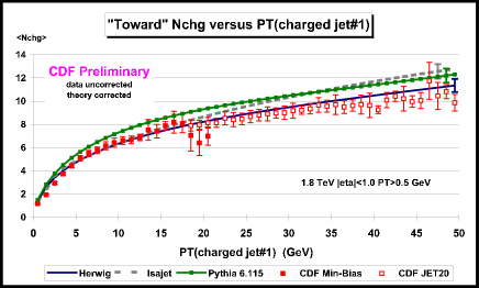
Figure 28: Data from Fig. 25 on the average number of charged particles ($p_{T}>0.5{\rm\,GeV}$ and $|\eta|<1$) as a function of $p_{T}({\rm jet\#1})$ (leading charged jet) for the “toward” region ” defined in Fig. 24 compared with the QCD “hard scattering” Monte-Carlo predictions of HERWIG 5.9, ISAJET 7.32, and PYTHIA 6.115. Each point corresponds to the “toward” $\langle N_{chg}\rangle$ in a $1{\rm\,GeV}$ bin. The errors on the (uncorrected) data include both statistical and correlated systematic uncertainties. The theory curves are corrected for the track finding efficiency and have an error (statistical plus systematic) of around $5\%$.

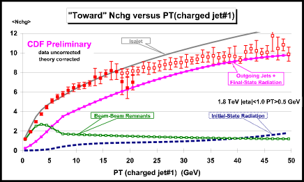
Figure 29: Data from Fig. 25 on the average number of charged particles ($p_{T}>0.5{\rm\,GeV}$ and $|\eta|<1$) as a function of $p_{T}({\rm jet\#1})$ (leading charged jet) for the “toward” region defined in Fig. 24 compared with the QCD ”hard scattering” Monte-Carlo predictions of ISAJET 7.32. The predictions of ISAJETare divided into three categories: charged particles that arise from the break-up of the beam and target (beam-beam remnants), charged particles that arise from initial-state radiation, and charged particles that result from the outgoing jets plus final-state radiation (see Fig. 19). The errors on the (uncorrected) data include both statistical and correlated systematic uncertainties. The theory curves are corrected for the track finding efficiency and have an error (statistical plus systematic) of around $5\%$.

Fig. 30 shows the data from Fig. 25 on the average number of “away” region charged particles compared with the QCD “hard scattering” Monte-Carlo predictions of HERWIG 5.9, ISAJET 7.32, and PYTHIA 6.115. In Fig. 21 the data from Fig. 26 on the average scalar $p_{T}$ sum in the “away” region is compared to the QCD Monte-Carlo predictions. The “away” region is a mixture of the underlying event and the “away-side” outgoing “hard scattering” jet. This can be seen in Fig. 32 where the predictions of ISAJET for the “away” region are divided into three categories: beam-beam remnants, initial-state radiation, and outgoing jets plus final-state radiation. Here the underlying event plays a more important role since the “away-side” outgoing “hard scattering” jet is sometimes outside the regions $|\eta|<1$. For the “toward” region the contribution from the outgoing jets plus final state-radiation dominates for $p_{T}({\rm jet\#1})$ values above about $5{\rm\,GeV}$, whereas for the “away” region this does not occur until around $20{\rm\,GeV}$.

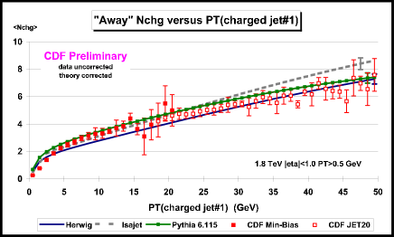
Figure 30: Data from Fig. 25 on the average number of charged particles ($p_{T}>0.5{\rm\,GeV}$ and $|\eta|<1$) as a function of $p_{T}({\rm jet\#1})$ (leading charged jet) for the “away” region defined in Fig. 24 compared with the QCD “hard scattering” Monte-Carlo predictions of HERWIG 5.9, ISAJET 7.32, and PYTHIA 6.115. The errors on the (uncorrected) data include both statistical and correlated systematic uncertainties. The theory curves are corrected for the track finding efficiency and have an error (statistical plus systematic) of around $5\%$.

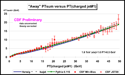
Figure 31: Data from Fig. 26 on the average scalar $p_{T}$ sum of charged particles (($p_{T}>0.5{\rm\,GeV}$ and $|\eta|<1$) as a function of $p_{T}({\rm jet\#1})$ (leading charged jet) for the “away” region defined in Fig. 24 compared with the QCD “hard scattering” Monte-Carlo predictions of HERWIG 5.9, ISAJET 7.32, and PYTHIA 6.115. The errors on the (uncorrected) data include both statistical and correlated systematic uncertainties. The theory curves are corrected for the track finding efficiency and have an error (statistical plus systematic) of around $5\%$.

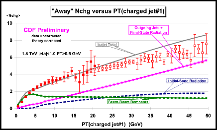
Figure 32: Data from Fig. 25 on the average number of charged particles ($p_{T}>0.5{\rm\,GeV}$ and $|\eta|<1$) as a function of $p_{T}({\rm jet\#1})$ (leading charged jet) for the “away” region defined in Fig. 24 compared with the QCD “hard scattering” Monte-Carlo predictions of ISAJET 7.32. The predictions of ISAJETare divided into three categories: charged particles that arise from the break-up of the beam and target (beam-beam remnants), charged particles that arise from initial-state radiation, and charged particles that result from the outgoing jets plus final-state radiation (see Fig. 19). The errors on the (uncorrected) data include both statistical and correlated systematic uncertainties. The theory curves are corrected for the track finding efficiency and have an error (statistical plus systematic) of around $5\%$.

Both the “toward” and “away” regions are described fairly well by the QCD “hard scattering” Monte-Carlo models. These regions are dominated by the outgoing “hard scattering” jets and as we saw in Section C the Monte-Carlo models describe the leading outgoing jets fairly accurately. We will now study the “transverse” region which is dominated by the underlying event.

8.5 The “Transverse” Region and the Underlying Event

Fig. 25 shows that there is a lot of activity in the “transverse” region. If we suppose that the “transverse” multiplicity is uniform in azimuthal angle $\phi$ and pseudo-rapidity $\eta$, the observed $2.3$ charged particles at $p_{T}({\rm jet\#1})=20{\rm\,GeV}$ translates to $3.8$ charged particles per unit pseudo-rapidity with $p_{T}>0.5{\rm\,GeV}$ (multiply by $3$ to get $360^{\circ}$, divide by $2$ for the two units of pseudo-rapidity, multiply by $1.09$ to correct for the track finding efficiency). We know that if we include all $p_{T}$ that there are roughly $4$ charged particles per unit rapidity in a “soft” $p\bar{p}$ collision at $1.8{\rm\,TeV}$, and the data show that in the underlying event of a “hard scattering” there are about $3.8$ charged particles per unit rapidity in the region $p_{T}>0.5{\rm\,GeV}$! If one includes all $p_{T}$ values then the underlying event has a charge particle density that is at least a factor of two larger than the $4$ charged particles per unit rapidity seen in “soft” $p\bar{p}$ collisions at this energy. As can be seen in Fig. 25, the charged particle density in the “transverse” region is a function of $p_{T}({\rm jet\#1})$ and rises very rapidity at low $p_{T}({\rm jet\#1})$ values. The “transverse” charged multiplicity doubles in going from $p_{T}({\rm jet\#1})=1.5{\rm\,GeV}$ to $p_{T}({\rm jet\#1})=2.5{\rm\,GeV}$ and then forms an approximately constant “plateau” for $p_{T}({\rm jet\#1})>6{\rm\,GeV}$.

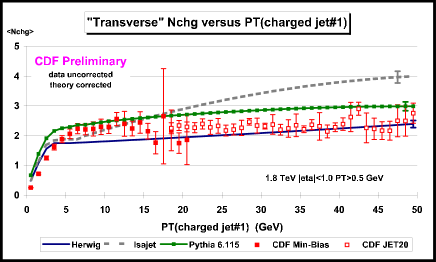
Figure 33: Data from Fig. 25 on the average number of charged particles ($p_{T}>0.5{\rm\,GeV}$ and $|\eta|<1$) as a function of $p_{T}({\rm jet\#1})$ (leading charged jet) for the “transverse” region defined in Fig. 24 compared with the QCD “hard scattering” Monte-Carlo predictions of HERWIG 5.9, ISAJET 7.32, and PYTHIA 6.115. The errors on the (uncorrected) data include both statistical and correlated systematic uncertainties. The theory curves are corrected for the track finding efficiency and have an error (statistical plus systematic) of around $5\%$.

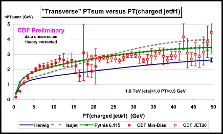
Figure 34: Data from Fig. 26 on the average scalar $p_{T}$ sum of charged particles ($p_{T}>0.5{\rm\,GeV}$ and $|\eta|<1$) as a function of $p_{T}({\rm jet\#1})$ (leading charged jet) for the “transverse” region defined in Fig. 24 compared with the QCD “hard scattering” Monte-Carlo predictions of HERWIG 5.9, ISAJET 7.32, and PYTHIA 6.115. The errors on the (uncorrected) data include both statistical and correlated systematic uncertainties. The theory curves are corrected for the track finding efficiency and have an error (statistical plus systematic) of around $5\%$.

Fig. 33 and Fig. 34 compare the “transverse” $\langle N_{chg}\rangle$ and the “transverse” $\langle{p_{T}}_{sum}\rangle$, respectively, with the QCD “hard scattering” Monte-Carlo predictions of HERWIG 5.9, ISAJET 7.32, and PYTHIA 6.115. Fig. 35 and Fig. 36 compare the “transverse” $\langle N_{chg}\rangle$ and the “transverse” $\langle PT_{sum}\rangle$, respectively, with three versions of PYTHIA(6.115, 6.125, and no multiple scattering, see Table 10). PYTHIA with no multiple parton scattering does not have enough activity in the underlying event. PYTHIA 6.115 fits the “transverse” $\langle N_{chg}\rangle$ the best, but overshoots slightly the “toward” $\langle N_{chg}\rangle$ in Fig. 28. ISAJET has a lot of activity in the underlying event, but gives the wrong $p_{T}({\rm jet\#1})$ dependence. Instead of a “plateau,” ISAJET predicts a rising “transverse” $\langle N_{chg}\rangle$ and gives too much activity at large $p_{T}({\rm jet\#1})$ values. HERWIG does not have enough “transverse” $\langle PT_{sum}\rangle$.

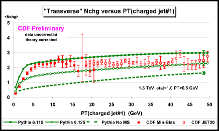
Figure 35: Data from Fig. 35 on the average number of charged particles ($p_{T}>0.5{\rm\,GeV}$ and $|\eta|<1$) as a function of $p_{T}({\rm jet\#1})$ (leading charged jet) for the “transverse” region defined in Fig. 24 compared with the QCD “hard scattering” Monte-Carlo predictions of PYTHIA 6.115, PYTHIA 6.125, and PYTHIA with no multiple parton scattering (No MS). The errors on the (uncorrected) data include both statistical and correlated systematic uncertainties. The theory curves are corrected for the track finding efficiency and have an error (statistical plus systematic) of around $5\%$.

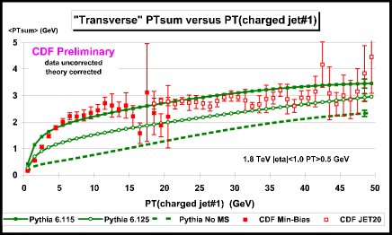
Figure 36: Data from Fig. 26 on the average scalar $p_{T}$ sum of charged particles ($p_{T}>0.5{\rm\,GeV}$ and $|\eta|<1$) as a function of $p_{T}({\rm jet\#1})$ (leading charged jet) for the “transverse” region defined in Fig. 24 compared with the QCD “hard scattering” Monte-Carlo predictions of PYTHIA 6.115, PYTHIA 6.125, and PYTHIA with no multiple parton scattering (No MS). The errors on the (uncorrected) data include both statistical and correlated systematic uncertainties. The theory curves are corrected for the track finding efficiency and have an error (statistical plus systematic) of around $5\%$.

We expect the “transverse” region to be composed predominately from particles that arise from the break-up of the beam and target and from initial-state radiation. This is clearly the case as can be seen in Fig. 37 where the predictions of ISAJET for the “transverse” region are divided into three categories: beam-beam remnants, initial- state radiation, and outgoing jets plus final-state radiation. It is interesting to see that it is the beam-beam remnants that are producing the approximately constant “plateau”. The contributions from initial-state radiation and from the outgoing hard scattering jets both increase as $p_{T}({\rm jet\#1})$ increases. In fact, for ISAJET it is the sharp rise in the initial-state radiation component that is causing the disagreement with the data for $p_{T}({\rm jet\#1})>20{\rm\,GeV}$.

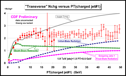
Figure 37: Data from Fig. 25 on the average number of charged particles ($p_{T}>0.5{\rm\,GeV}$ and $|\eta|<1$) as a function of $p_{T}({\rm jet\#1})$ (leading charged jet) for the “transverse” region defined in Fig. 24 compared with the QCD “hard scattering” Monte-Carlo predictions of ISAJET 7.32. The predictions of ISAJETare divided into three categories: charged particles that arise from the break-up of the beam and target (beam-beam remnants), charged particles that arise from initial-state radiation, and charged particles that result from the outgoing jets plus final-state radiation (see Fig. 19). The errors on the (uncorrected) data include both statistical and correlated systematic uncertainties. The theory curves are corrected for the track finding efficiency and have an error (statistical plus systematic) of around $5\%$.

As we explained in Section B, for HERWIG and PYTHIA it makes no sense to distinguish between particles that arise from initial-state radiation from those that arise from final-state radiation, but one can separate the “hard scattering component” from the beam-beam remnants. For PYTHIA the beam-beam remnants include contributions from multiple parton scattering as illustrated in Fig. 19. Fig. 38 and Fig. 39 compare the “transverse” $\langle N_{chg}\rangle$ with the QCD “hard scattering” Monte-Carlo predictions of HERWIG 5.9 and PYTHIA 6.115, respectively. Here the predictions are divided into two categories: charged particles that arise from the break-up of the beam and target (beam-beam remnants), and charged particles that result from the outgoing jets plus initial and final-state radiation (hard scattering component). As was the case with ISAJET the beam-beam remnants form the approximately constant “plateau” and the hard scattering component increase as $p_{T}({\rm jet\#1})$ increases. However, the hard scattering component of HERWIG and PYTHIA does not rise nearly as fast as the hard scattering component of ISAJET. This can be seen clearly in Fig. 40 where we compare directly the hard scattering component (outgoing jets plus initial and final-state radiation) of the “transverse” $\langle N_{chg}\rangle$ from ISAJET 7.32, HERWIG 5.9, and PYTHIA 6.115. PYTHIA and HERWIG are similar and rise gently as $p_{T}({\rm jet\#1})$ increases, whereas ISAJETproduces a much sharper increase as $p_{T}({\rm jet\#1})$ increases.

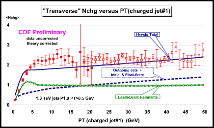
Figure 38: Data from Fig. 25 on the average number of charged particles ($p_{T}>0.5{\rm\,GeV}$ and $|\eta|<1$) as a function of $p_{T}({\rm jet\#1})$ (leading charged jet) for the “transverse” region defined in Fig. 24 compared with the QCD “hard scattering” Monte-Carlo predictions of HERWIG 5.9. The predictions of HERWIG are divided into two categories: charged particles that arise from the break-up of the beam and target (beam-beam remnants), and charged particles that result from the outgoing jets plus initial and final-state radiation (hard scattering component) (see Fig. 19). The errors on the (uncorrected) data include both statistical and correlated systematic uncertainties. The theory curves are corrected for the track finding efficiency and have an error (statistical plus systematic) of around $5\%$.

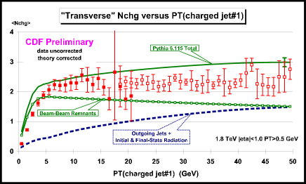
Figure 39: Data from Fig. 25 on the average number of charged particles ($p_{T}>0.5{\rm\,GeV}$ and $|\eta|<1$) as a function of $p_{T}({\rm jet\#1})$ (leading charged jet) for the “transverse” region defined in Fig. 24 compared with the QCD “hard scattering” Monte-Carlo predictions of PYTHIA 6.115. The predictions of PYTHIA are divided into two categories: charged particles that arise from the break-up of the beam and target (beam-beam remnants), and charged particles that result from the outgoing jets plus initial and final-state radiation (hard scattering component). For PYTHIA, the beam-beam remnants include contributions from multiple parton scattering (see Fig. 19). The errors on the (uncorrected) data include both statistical and correlated systematic uncertainties. The theory curves are corrected for the track finding efficiency and have an error (statistical plus systematic) of around $5\%$.

There are two reasons why the hard scattering component of ISAJET is different from HERWIG and PYTHIA. The first is due to different fragmentation schemes. ISAJET uses independent fragmentation, which produces too many soft hadrons when partons begin to overlap. The second difference arises from the way the QCD Monte-Carlo produce “parton showers”. ISAJET uses a leading-log picture in which the partons within the shower are ordered according to their invariant mass. Kinematics requires that the invariant mass of daughter partons be less than the invariant mass of the parent. HERWIG and PYTHIA modify the leading-log picture to include “color coherence effects” which leads to “angle ordering” within the parton shower. Angle ordering produces less high $p_{T}$ radiation within a parton shower which is what is seen in Fig. 40. Without further study, we do not know how much of the difference seen in Fig. 40 is due to the different fragmentation schemes and how much is due to the color coherence effects.

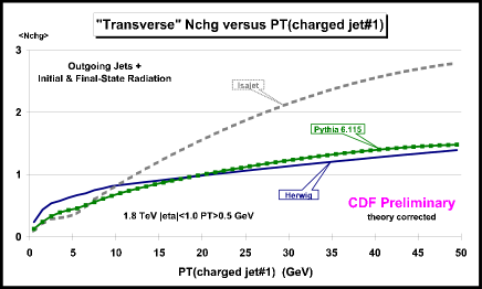
Figure 40: QCD “hard scattering” Monte-Carlo predictions from HERWIG 5.9, ISAJET 7.32, and PYTHIA 6.115 of the average number of charged particles ($p_{T}>0.5{\rm\,GeV}$ and $|\eta|<1$) as a function of $p_{T}({\rm jet\#1})$ (leading charged jet) for the “transverse” region defined in Fig. 24 arising from the outgoing jets plus initial and finial-state radiation (hard scattering component). The curves are corrected for the track finding efficiency and have an error (statistical plus systematic) of around $5\%$.

The beam-beam remnant contribution to the “transverse” $\langle N_{chg}\rangle$ is different for each of the QCD Monte- Carlo models. This can be seen in Fig. 41 where we compare directly the beam-beam remnant component of the “transverse” $\langle N_{chg}\rangle$ from ISAJET 7.32, HERWIG 5.9, PYTHIA 6.115, and PYTHIA with no multiple parton interactions. Since we are considering only charged particles with $p_{T}>0.5{\rm\,GeV}$, the height of the “plateaus” in Fig. 41 is related to the $p_{T}$ distribution of the beam-beam remnant contributions. A steeper $p_{T}$ distribution means less particles with $p_{T}>0.5{\rm\,GeV}$. PYTHIA uses multiple parton scattering to enhance the underlying event and we have included these contributions in the beam-beam remnants. For PYTHIA the height of the “plateau” in Fig. 41 can be adjusted by adjusting the amount of multiple parton scattering. HERWIG and ISAJET do not include multiple parton scattering. For HERWIG and ISAJET the height of the “plateau” can be adjusted by changing the $p_{T}$ distribution of the beam-beam remnants.

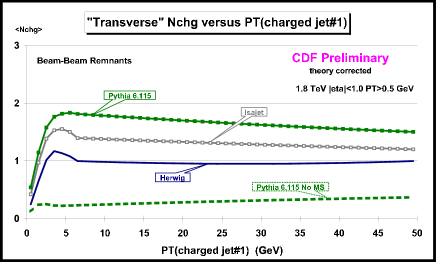
Figure 41: QCD “hard scattering” Monte-Carlo predictions from HERWIG 5.9, ISAJET 7.32, PYTHIA 6.115, and PYTHIA  with no multiple parton scattering (No MS) of the average number of charged particles ($p_{T}>0.5{\rm\,GeV}$ and $|\eta|<1$) as a function of $p_{T}({\rm jet\#1})$ (leading charged jet) for the “transverse” region defined in Fig. 7 arising from the break-up of the beam and target (beam-beam remnants). For PYTHIA the beam-beam remnants include contributions from multiple parton scattering (see Fig. 19). The curves are corrected for the track finding efficiency and have an error (statistical plus systematic) of around $5\%$.

8.6 Summary and Conclusions

For $p\bar{p}$ collisions at $1.8{\rm\,TeV}$ min-bias does not necessarily imply “soft” physics. There is a lot of QCD “hard scattering” in the Min-Bias data. We have studied both “local” leading jet observables and “global” observables where to fit the data the QCD Monte-Carlo models have to correctly describe the entire event structure. Our summary and conclusions are as follows.

The Evolution of Charge Particle Jets

Charged particle jets are “born” somewhere around $p_{T}({\rm jet})$ of about $2{\rm\,GeV}$ with, on the average, about $2$ charged particles and grow to, on the average, about $10$ charged particles at $50{\rm\,GeV}$. The QCD “hard scattering” models describe quite well (although not perfectly) “local” leading jet observables such as the multiplicity distribution of charged particles within the leading jet, the “size” of the leading jet, the radial flow of charged particles and $p_{T}$ around the leading jet direction, and the momentum distribution of charged particles within the leading jet. In fact, the QCD “hard” scattering Monte-Carlo models agree as well with $2{\rm\,GeV}$ charged particle jets as they do with $50{\rm\,GeV}$ charged particle jets! The charge particle jets in the Min-Bias data are simply the extrapolation (down to small $p_{T}$) of the high $p_{T}$ jets observed in the JET20 data. For a fixed $p_{T}({\rm hard})$, the QCD “hard” scattering cross section grows with increasing collider energy. As the center-of-mass energy of a $p\bar{p}$ collision grows, “hard” scattering becomes a larger and larger fraction of the total inelastic cross section. At $1.8{\rm\,TeV}$ “hard scattering” makes up a sizable part of the “hard core” inelastic cross section and a lot of min-bias events have $2{\rm\,TeV}$ or $3{\rm\,GeV}$ jets.

The “Underlying Event”

A hard scattering collider event consists of large $p_{T}$ outgoing hadrons that originate from the large $p_{T}$ partons (outgoing jets) and also hadrons that originate from the break-up of the proton and antiproton (beam-beam remnants). The “underlying event” is formed from the beam-beam remnants, initial-state radiation, and possibly from multiple parton interactions. Our data show that the charged particle multiplicity and scalar $p_{T}$ sum in the “underlying event” grows very rapidly with the transverse momentum of the leading charged particle jet and then forms an approximately constant “plateau” for $p_{T}({\rm jet\#1})>6{\rm\,GeV}$. The height of this“plateau” is at least twice that observed in “soft” collisions at the same corresponding energy.

None of the QCD Monte-Carlo models we examined correctly describe all the properties of the underlying event seen in the data. HERWIG 5.9 and PYTHIA 6.125 do not have enough activity in the underlying event. PYTHIA  6.115 has about the right amount of activity in the underlying event, but as a result produces too much overall charged multiplicity. ISAJET 7.32 has a lot of activity in the underlying event, but with the wrong dependence on $p_{T}({\rm jet\#1})$. Because ISAJET uses independent fragmentation and HERWIG and PYTHIA do not, there are clear differences in the hard scattering component (mostly initial-state radiation) of the underlying event between ISAJET and the other two Monte-Carlo models. Here the data strongly favor HERWIG and PYTHIA over ISAJET.

The beam-beam remnant component of both ISAJET 7.32 and HERWIG 5.9 has the wrong $p_{T}$ dependence. ISAJET and HERWIG both predict too steep of a $p_{T}$ distribution. PYTHIA does a better job, but is still slightly too steep. It is, of course, understandable that the Monte-Carlo models might be somewhat off on the parameterization of the beam-beam remnants. This component cannot be calculated from perturbation theory and must be determined from data. With what we have learned from the data presented here, the beam-beam remnant component of the QCD “hard scattering” Monte-Carlo models can be tuned to better describe the overall event in $p\bar{p}$ collisions.

References

- [1] G. Marchesini, B.R. Webber, G. Abbiendi, I.G. Knowles, M.H. Seymour and L. Stanco, Comput. Phys. Commun. 67 (1992) 465.
- [2] F.E. Paige, S.D. Protopescu, H. Baer and X. Tata, hep-ph/9810440.
- [3] T. Sjöstrand, Comput. Phys. Commun. 82 (1994) 74.
-
[4]
G. Bodwin, Phys. Rev. D31 (1985) 2616;
J.C. Collins, D.E. Soper, G. Sterman, Nucl. Phys. B261 (1985) 104. - [5] M. Bengtsson, T. Sjöstrand and M. van Zijl, Z. Phys. C32 (1986) 67.
-
[6]
V.N. Gribov and L.N. Lipatov, Sov. J. Nucl. Phys. 15 (1972) 438;
G. Altarelli and G. Parisi, Nucl. Phys. B126 (1977) 298;
Yu.L. Dokshitzer, Sov. Phys. JETP 46 (1977) 641. - [7] R. Odorico, Nucl. Phys. B172 (1980) 157.
- [8] R.K. Ellis, W.J. Stirling and B. Webber, “QCD and Collider Physics,” Cambridge University Press (UK) 1996.
- [9] T. Sjöstrand, Phys. Lett. 157B (1985) 321.
-
[10]
G. Marchesini and B.R. Webber, Nucl. Phys. B238 (1984) 1;
B.R. Webber, Ann. Rev. Nucl. Part. Sci. 36 (1986) 253. - [11] Y.I. Dokshitzer, D.I. D’Yakonov, S.I. Troyan, Phys. Lett. B79 (1978) 269.
- [12] G. Parisi, R. Petronzio, Nucl. Phys. B154 (1979) 427.
- [13] S.D. Ellis, N. Fleishon, and W.J. Stirling, Phys. Rev. D24 (1981) 1386.
- [14] J. Collins, D. Soper, Nucl. Phys. B193 (1981) 381; Erratum B213 (1983) 545; B197 (1982) 446.
- [15] J. Collins, D. Soper, G. Sterman, Nucl. Phys. B250 (1985) 199.
- [16] G. Altarelli, R.K. Ellis, M. Greco, G. Martinelli, Nucl. Phys. B246 (1984) 12.
- [17] G. Altarelli, R.K. Ellis, G. Martinelli, Z. Phys. C27 (1985) 617.
- [18] P.B. Arnold, R.P. Kauffman, Nucl. Phys. B349 (1991) 381.
- [19] R.K. Ellis, S. Veseli, Nucl. Phys. B511 (1998) 649.
- [20] A. Kulesza and W.J. Stirling, eprint [hep-ph/9902234].
- [21] J. Kodaira and L. Trentadue, Phys. Lett. 112B (1982) 66.
- [22] C. Balázs, C.P. Yuan, Phys. Rev. D56 (1997) 5558.
- [23] H. Baer and M.H. Reno, Phys. Rev. D44 (1991) 3375, D45 (1992) 1503.
-
[24]
J. André and T. Sjöstrand, Phys. Rev. D57 (1998) 5767;
G. Ingelman, in Physics at HERA, Vol. 3, p. 1366;
M.H. Seymour, Zeit. Phys. C56 (1992) 161. -
[25]
M. Bengtsson and T. Sjöstrand, Phys. Lett. B185 (1987) 435;
G. Gustafson and U. Pettersson, Nucl. Phys. B306 (1988) 746;
L. Lönnblad, Comput. Phys. Commun. 71 (1992) 15;
M.H. Seymour, preprint LU TP 94-12, International Conference on High Energy Physics, Glasgow, U.K., 20–27 July 1994; Nucl. Phys. B436 (1995) 443;
G. Corcella and M.H. Seymour, Phys. Lett. B442 (1998) 417. -
[26]
G. Miu, eprint [hep-ph/9804317];
G. Miu and T. Sjöstrand, eprint [hep-ph/9912455] - [27] DØ Collaboration, S. Abachi et al., Phys. Rev. Lett. 80 (1998) 5498.
- [28] CDF Collaboration, T. Affolder et al., Phys. Rev. Lett. 84 (2000) 845.
-
[29]
S. Frixione, M.L. Mangano, P. Nason and G. Ridolfi,
Nucl. Phys. B431 (1994) 453;
L. Apanasevich et al., eprint [hep-ph/9808467]. - [30] C. Balázs, J.W. Qui, C.–P. Yuan, Phys. Lett. B355 (1995) 548.
- [31] R. Meng, F.I. Olness, D.E. Soper, Phys. Rev. D54 (1996) 1919.
-
[32]
N. Kidonakis, G. Sterman, Nucl. Phys. B505 (1997) 321;
R. Bonciani, S. Catani, M. Mangano, P. Nason, Nucl. Phys. B529 (1998) 424;
N. Kidonakis, G. Oderda, G. Sterman, Nucl. Phys. B531 (1998) 365;
S. Catani, M. Mangano, P. Nason, JHEP 9807: 024 (1998). - [33] P.B. Arnold, M.H. Reno, Nucl. Phys. B319 (1989) 37; Erratum B330 (1990) 284.
- [34] S. Mrenna, Comput. Phys. Commun. 101 (1997) 232.
- [35] H.L. Lai, J. Huston, S. Kuhlmann, J. Morfín, F. Olness, J. Owens, J. Pumplin, W.K. Tung, hep-ph/9903282.
- [36] P. Edén and G. Gustafson, Z. Phys. C75 (1997) 41.
- [37] C. Friberg and T. Sjöstrand, LU TP 99–11 and hep-ph/9907245, to appear in Eur. Phys. J. C.
- [38] M. Bengtsson and T. Sjöstrand, Phys. Lett. B185 (1987) 435; G. Gustafson and U. Pettersson, Nucl. Phys. B306 (1988) 746; M.H. Seymour, Comput. Phys. Commun. 90 (1995) 95.
- [39] G. Miu and T. Sjöstrand, Phys. Lett. B449 (1999) 313.
- [40] J. Huston, these proceedings.
- [41] G. Corcella and M.H. Seymour, RAL-TR-1999-051 and hep-ph/9908388.
- [42] S. Mrenna, UCD-99-4 and hep-ph/9902471.
- [43] S. Mrenna, in preparation.
- [44] J. André and T. Sjöstrand, Phys. Rev. D57 (1998) 5767.
- [45] C. Friberg and T. Sjöstrand, in ‘Monte Carlo Generators for HERA Physics’, eds. A.T. Doyle, G. Grindhammer, G. Ingelman and H. Jung, DESY-PROC-1999-02, p. 181.
- [46] WA82 Collaboration, M. Adamovich et al., Phys. Lett. B305 (1993) 402; E769 Collaboration, G.A. Alves et al., Phys. Rev. Lett. 72 (1994) 812; E791 Collaboration, E.M. Aitala et al., Phys. Lett. B371 (1996) 157.
- [47] E. Norrbin and T. Sjöstrand, Phys. Lett. B442 (1998) 407, in preparation.
- [48] B. Andersson, G. Gustafson, G. Ingelman and T. Sjöstrand, Phys. Rep. 97 (1983) 31; T. Sjöstrand, Nucl. Phys. B248 (1984) 469.
- [49] T. Sjöstrand and M. van Zijl, Phys. Rev. D36 (1987) 2019.
- [50] CDF collaboration, F. Abe et al., Phys. Rev. Lett. 79 (1997) 584.
- [51] G. Gustafson and G. Miu, LU TP 99–43.
- [52] J. Dischler and T. Sjöstrand, in preparation.
- [53] A. Donnachie and P.V. Landshoff, Phys. Lett. B296 (1992) 227.
- [54] G. Gustafson, U. Pettersson and P. Zerwas, Phys. Lett. B209 (1988) 90.
- [55] T. Sjöstrand and V.A. Khoze, Z. Phys. C62 (1994) 281, Phys. Rev. Lett. 72 (1994) 28.
- [56] G. Gustafson and J. Häkkinen, Z. Phys. C64 (1994) 659; L. Lönnblad, Z. Phys. C70 (1996) 107; Š. Todorova–Nová, DELPHI Internal Note 96-158 PHYS 651; J. Ellis and K. Geiger, Phys. Rev. D54 (1996) 1967, Phys. Lett. B404 (1997) 230; B.R. Webber, J. Phys. G24 (1998) 287.
- [57] J. Häkkinen and M. Ringnér, Eur. Phys. J. C5 (1998) 275.
- [58] L. Lönnblad and T. Sjöstrand, Phys. Lett. B351 (1995) 293, Eur. Phys. J. C2 (1998) 165.
- [59] S. Jadach and K. Zalewski, Acta Phys. Pol. B28 (1997) 1363; V. Kartvelishvili, R. Kvatadze and R. Møller, Phys. Lett. B408 (1997) 331; K. Fiałkowski and R. Wit, Acta Phys. Pol. B28 (1997) 2039, Eur. Phys. J. C2 (1998) 691; Š. Todorova–Nová and J. Rameš, hep-ph/9710280.
- [60] V.A. Khoze and T. Sjöstrand, Phys. Lett. B328 (1994) 466.
- [61] A. Edin, G. Ingelman and J. Rathsman, Z. Phys. C75 (1997) 57.
- [62] A. Edin, G. Ingelman and J. Rathsman, Phys.Rev. D56 (1997) 7317.
- [63] L. Lönnblad, Comput. Phys. Commun. 118 (1999) 213.
-
[64]
http://fnth37.fnal.gov/susy.html -
[65]
http://runIIcomputing.fnal.gov/strongdynamics/web/strongdynamics.html -
[66]
http://fnth37.fnal.gov/higgs/draft.html -
[67]
http://fnth37.fnal.gov/sugra.html -
[68]
http://b0nd10.fnal.gov/~regina/tcolor.html -
[69]
http://www-theory.fnal.gov/people/bdob/dimensions.html - [70] F. Abe et al., “Evidence for top quark production in collisions at TeV,” Phys. Rev. D50 (1994) 2966.
- [71] F. Abe et al., “Search for Scalar Top and Scalar Bottom in collisions at TeV,” hep-ex/9912018, submitted to Phys. Rev. Lett.
- [72] J.M. Campbell, R.K. Ellis (Fermilab) This proceedings.
- [73] F. Abe et al., “Measurement of Correlated Jet Cross Sections in Collisions at TeV,” Phys. Rev. D53 (1996) 1051.
- [74] F. Abe et al., “A Measurement of the Bottom Quark Production Cross Section in 1.8 TeV Collisions Using Semileptonic Decay Muons,” Phys. Rev. Lett. 71 (1993) 2396.
- [75] T. Nakaya, “Measurement of the production cross section in collisions at TeV,” report CDF-ANAL-BOTTOM-CDFR-5025.
- [76] F. Abe et al., “Measurement of the B0 anti-B0 Oscillation Frequency Using pi-B Meson Charge-Flavor Correlations in Collisions at TeV,” Phys. Rev. Lett. 80 (1998) 2057; F. Abe et al., “A Measurement of the B Meson and b Quark Cross Section at TeV Using the Exclusive Decay ,” Phys. Rev. D50 (1994) 4252; F. Abe et al., “A Measurement of the B Meson and b Quark Cross Section at TeV Using the Exclusive Decay ,” Phys. Rev. Lett. 68 (1992) 3403.
-
[77]
http://www-theory.fnal.gov/people/ellis/Talks/top.ps.gz -
[78]
See the references at
http://www-d0.fnal.gov/~heinson/thinkshop/singletop_papers_thinkshop.html - [79] J.M. Campbell, R.K. Ellis, Phys. Rev. D60 (1999) 113006.
- [80] T.Adams et al., in Proceedings of the 33rd Rencontres de Moriond, QCD and Hadronic Interactions, (to be published), hep-ex/9906037.
- [81] S.A.Rabinowitz et al., Phys. Rev. Lett. 70 (1993) 134.
- [82] P. Vilain et al., Eur. Phys. J. C11 (1999) 19.
- [83] H. Abramowicz et al., Z. Phys. C15 (1982) 19.
- [84] M. Gluck, E. Reya, A. Vogt, “Dynamic parton distributions of the proton and small-x physics,” Z. Phys. C67 (1995) 433.
- [85] H.L. Lai, et al., “Improved Parton Distributions from Global Analysis of Recent Deep Inelastic Scattering and Inclusive Jet Data,” Phys. Rev. D55 (1997) 1280.
- [86] F. Abe et al., “Search for New Particles Decaying into and Produced in Association with Bosons Decaying into and at the Tevatron,” Phys. Rev. Lett. 79 (1997) 3819.
- [87] E. Laenen, S. Riemersma, J. Smith and W.L. van Neerven, Nucl. Phys. B392 (1993) 162; ibid. (1993) 229.
- [88] J. Collins, F. Wilczek and A. Zee, Phys. Rev. D18 (1978) 242.
- [89] S. Riemersma, J. Smith and W.L. van Neerven, Phys. Lett. B347 (1995) 43.
- [90] M. Buza, Y. Matiounine, J. Smith, R. Migneron and W.L. van Neerven, Nucl. Phys. B472 (1996) 611.
- [91] B.W. Harris and J. Smith, Nucl. Phys. B452 (1995) 109.
- [92] J. Breitweg et al. (ZEUS Collaboration), Phys. Lett. B407 (1997) 402, hep-ex/9908012.
- [93] C. Adloff et al. (H1-collaboration), Nucl. Phys. B545 (1999) 21.
- [94] M. Buza, Y. Matiounine, J. Smith, W.L. van Neerven, Eur. Phys. J. C1 (1998) 301.
- [95] W.L. van Neerven and E.B. Zijlstra, Phys. Lett. B272 (1991) 127, E.B. Zijlstra and W.L. van Neerven, Phys. Lett. B273 (1991) 476, Nucl. Phys. B383 (1992) 525.
- [96] P.J. Rijken and W.L. van Neerven, Phys. Rev. D51 (1995) 44.
- [97] A. Chuvakin, J. Smith and W.L. van Neerven, hep-ph/9910250.
-
[98]
M. Buza, Y. Matiounine, J. Smith, W.L. van Neerven,
Phys. Lett. B411 (1997) 211;
W.L. van Neerven, Acta Phys. Polon. B28 (1997) 2715;
W.L. van Neerven in Proceedings of the 6th International Workshop on Deep Inelastic Scattering and QCD ”DIS98” edited by GH. Coremans and R. Roosen, (World Scientific, 1998), p. 162-166, hep-ph/9804445;
J. Smith in New Trends in HERA Physics, edited by B.A. Kniehl, G. Kramer and A. Wagner, (World Scientific, 1998), p. 283, hep-ph/9708212. - [99] M.A.G. Aivazis, J.C. Collins, F.I. Olness and W.-K. Tung, Phys. Rev. D50 (1994) 3102; F. Olness and S. Riemersma, Phys. Rev. D51 (1995) 4746.
- [100] J.C. Collins, Phys. Rev. D58 (1998) 0940002.
- [101] R.S. Thorne and R.G. Roberts, Phys. Lett. B421 (1998) 303; Phys. Rev. D57 (1998) 6871.
- [102] M. Glück, E. Reya and A. Vogt, Eur. Phys. J. C5 (1998) 461.
- [103] W.L. van Neerven and J.A.M. Vermaseren, Nucl. Phys. B238 (1984) 73; See also S. Kretzer and I. Schienbein, Phys. Rev. D58 (1998) 094035.
- [104] F.A. Berends, G.J.J. Burgers and W.L. van Neerven, Nucl. Phys. B297 (1988) 429 ; Erratum ibid. Nucl. Phys. B304 (1988) 921.
- [105] A. Chuvakin, J. Smith, hep-ph/9911504.
- [106] A.D. Martin, R.G. Roberts, W.J. Stirling and R. Thorne, Eur. Phys. J. C4 (1998) 463.
- [107] A. Chuvakin, J. Smith and W.L. van Neerven, in preparation.
- [108] ATLAS Detector and Physics Performance Technical Design Report, CERN/LHCC/99-14.
- [109] C. Schmidt, private communication.
- [110] S. Catani and B.R. Webber, Nucl. Phys. B349 (1991) 635.
- [111] C. Balazs and C. P. Yuan, Phys. Rev. D56, 5558 (1997) hep-ph/9704258; C. Balazs and C. P. Yuan, hep-ph/0001103.
- [112] H.L. Lai, J. Huston, S. Kuhlmann, F. Olness, J. Owens, D. Soper, W.K. Tung, H. Weerts, Phys. Rev. D55 (1997) 1280.
- [113] G. Corcella, talk at the LHC workshop, October 1999.
- [114] G. Ladinsky, C.P. Yuan, Phys. Rev. D50 (1994) 4239.
- [115] C. Balazs, J. Collins and D. Soper, these proceedings.
- [116] F. Abe et al., Phys. Rev. Lett. 70 (1993) 2232; T. Takano, Ph.D. thesis, U. Tsukuba (1998); CDF Collaboration, paper in preparation.
- [117] C. Balazs, P. Nadolsky, C. Schmidt and C.–P. Yuan, hep-ph/9905551.
- [118] P. Aurenche, A. Douri, R. Baier, M. Fontannaz, Z. Phys. C29 (1985) 423; B. Bailey, J. Owens, J. Ohnemus, Phys. Rev. D46 (1992) 2018; T. Binoth, J.P. Guillet, E. Pilon, M. Werlen, hep-ph/9911340.
- [119] PYTHIA manual update for version 6.1.
- [120] D. Denegri, private communication.
- [121] S. Mrenna, talk at the Run 2 workshop, Nov 1999, Fermilab; C. Balazs, J. Huston, S. Mrenna, I. Puljak, Proceedings of the Run 2 Workshop.
- [122] F. Abe et al., Nucl. Instrum. Methods, A271 (1988) 387.
- [123] R.K. Ellis and Sinisa Veseli, Phys.Rev. D60 (1999) 011501.
-
[124]
Z. Bern, L. Dixon, D. Kosower and S. Weinzierl,
Nucl. Phys. B489 (1997) 3;
Z. Bern, L. Dixon and D. Kosower, Nucl. Phys. B513 (1998) 3. - [125] L. Dixon, Z. Kunszt and A. Signer, Nucl. Phys. B531 (1998) 3.
- [126] R.K. Ellis, D.A. Ross and A.E. Terrano, Nucl. Phys. B178 (1981) 421.
- [127] S. Catani and M.H. Seymour, Nucl. Phys. B485 (1997) 291, Erratum, ibid B510 (1997) 503.
- [128] G. Altarelli, R.K. Ellis and G. Martinelli, Nucl. Phys. B157 (1979) 461.
- [129] J. Kubar, M. Le Bellac, J.L. Meunier, G. Plaut, Nucl. Phys.B175 (1980) 251.
- [130] H. Georgi, Nucl. Phys.B363 (1991) 301.
- [131] A.D. Martin, R.G. Roberts, W.J. Stirling, R.S. Thorne, eprint [hep-ph/9907231]
-
[132]
S. Kim, S. Kuhlmann and W.M. Yao,
presented at 1996 DPF/DPB Summer Study on New Directions
for High-energy Physics (Snowmass 96), Snowmass, CO, July 1996;
P. Agrawal, D. Bowser-Chao and K. Cheung, Phys. Rev. D51 (1995) 6114. - [133] J.C. Collins and D. Soper, Phys. Rev. D16 (1977) 2219.