Spiral Multi-component Structure in Padé - Approximant QCD

Abstract

We present a graphical method of analyzing the infra-red fixed point structure of Padé approximant QCD. The analysis shows a spiral multi-component couplant structure as well as an infra-red attractor behavior of PQCD couplant for all flavors $0\leq N_{f}\leq 16$.

Keywords: Padé QCD couplant multiplicity structure
PACS: 12.38.-t
E-mail: ndili@hbar.rice.edu

1 INTRODUCTION

In two recent papers Elias et. al. [1, 2] showed that by analyzing the sequence of occurrence of the first zeros of the denominator and numerator of a Padé approximant beta function, one can separate out two possible behaviors of Padé QCD couplant in the infra-red (IR) region. The couplant may exhibit an IR attractor behavior of Kogan-Shifman type [3] in which the PQCD couplant bifurcates at some critical cut-off momentum $\mu_{c}$ into a second (upper) branch, in a manner that leaves the infra-red region $0\leq\mu<\mu_{c}$ totally free of any PQCD color force and its bifurcated branch. We may call this scenario II. The alternative scenario I is that the PQCD couplant freezes at the critical momentum point $\mu=\mu_{c}$, being its stable infra-red fixed point, and remains so frozen for all $0\leq\mu<\mu_{c}$ in the manner of Mattingly-Stevenson [4, 5].

The finding of Elias et. al. by their denominator-numerator zero approach is that scenario II holds for all $0\leq N_{f}\leq 5$, regardless of which Padé approximants, $[1|2],[2|1],[1|3],[3|1]$, or $[2|2]$ they used. On the other hand, they found that scenario I holds for all $9\leq N_{f}\leq 16$. For the flavor numbers, $N_{f}=6,7,8$, their method led to indeterminate results. Their positive denominator zeros ceased to exist for $N_{f}\geq 6$, but then their numerator zeros were found to be negative for $N_{f}=6,7,8$. As a result their method did not resolve the above question for these flavor states of Padé QCD.

We have re-examined the above question, using a graphical method to analyze the Padé QCD couplant equation of evolution, and applying this not only to the NNNLO $[2|1],[1|2]$ Padé approximants studied by Elias et. al. but also to the optimized $[1|1]$ Padé approximant more directly related to the optimized NNLO truncated PQCD beta function studied by Mattingly and Stevenson.

While confirming some of the findings of Elias et. al., we found substantially new features. In particular, we found for all flavors, not just the Elias et. al. bifurcation at momentum point $Q=\mu=\mu_{c}=Q_{\mathrm{min}}$, but a second bifurcation at $Q=\mu=Q_{\mathrm{max}}$, where in all cases $Q_{\mathrm{max}}>Q_{\mathrm{min}}$. More explicitly, we found the Padé couplant equation yielding three independent solutions or component couplants $a_{1},a_{2},a_{3}$ that are however joined together into a continuous chain-like spiral structure at the two momentum points $Q_{\mathrm{min}}$ and $Q_{\mathrm{max}}$ that can be called couplant bifurcation points.

The $a_{3}$ solution arising from the second bifurcation, is found to increase towards lower energies, running past the original PQCD bifurcation point at $Q=\mu_{c}$, into the region $\mu<\mu_{c}$, the implication being that this $a_{3}$ second bifurcation upper branch is either a genuine NPQCD component, or else a persisting Landau pole structure coming from the original truncated PQCD beta function on which the Padé beta function was based.

By noting from our graphical structures and plots, that the momentum gap $0\leq Q<Q_{\mathrm{min}}$ is not zero for all $9\leq N_{f}\leq 16$, we found that scenario II actually holds also for the flavor states $9\leq N_{f}\leq 16$ as for all $0\leq N_{f}\leq 8$, in difference to the findings of Elias et. al. The only amplification is that one has to go to sufficiently low momentum to see the persisting infra-red attractor points at $\mu=\mu_{c}=Q_{\mathrm{min}}$. This apart, the gap $0\leq\mu<\mu_{c}$ remains finite and empty of any PQCD couplant even for the highest flavors $N_{f}=16,15,14..$. The result is our new feature that there is intrinsically in Padé QCD, no couplant freezing for all flavors $0\leq N_{f}\leq 16$.

We present the above analysis and findings as follows. In section 2, we collect together the basic QCD couplant equations we need, together with their Padé approximants, and the optimized formulation of the particular NNLO Padé beta function. In section 3 , we present our numerical and graphical method of solving the Padé QCD couplant equations of orders $[1|1],[2|1],[1|2]$ that we considered. Then in sections 4 and 5, we state the main features and results we found with these Padé QCDs. In section 6, we use our graphical method to show explicitly that infra-red scenario II holds intrinsically for all flavors $0\leq N_{f}\leq 16$. In section 7, we relate our results and findings to the IR fixed point results of Banks and Zaks [6], and Stevenson et. al. [4, 5, 7, 8]. Our summary and conclusions are stated in section 8.

2 BASIC QCD COUPLANT EQUATIONS AND THEIR PADÉ APPROXIMANTS

2.1 The basic dynamical Equation of evolution of QCD coupling Constant

The starting point is the basic RG dynamical equation of evolution of QCD coupling constant given by:

$$\mu\frac{\partial\alpha_{s}(\mu)}{\partial\mu}=\beta(\alpha_{s}(\mu))$$ (1)

where $\mu$ is some arbitrary energy renormalization scale, and $\beta(\alpha_{s}(\mu))$ is the (abstract) QCD beta function. Eqn. (1) as it stands is believed to have a universal validity for all of QCD, that is to hold over a wide range of values of momentum scale $\mu$, except if the beta function is later specially parameterized or truncated. In the asymptotically free (AF) region of QCD, the beta function is parameterized in the perturbation series form:

$$\beta(a)=-ba^{2}(1+ca+c_{2}a^{2}+c_{3}a^{3}+c_{4}a^{4}+\cdots\rightarrow\infty)$$ (2)

where $a$ is the QCD coupling constant in the form $a=\alpha_{s}/\pi$, while the first few expansion coefficients $b,c,c_{2},c_{3}$ have the specific values [9, 10, 11]:

$$b=\frac{33-2N_{f}}{6}=2\beta_{0}$$ (3)

$$c=\frac{153-19N_{f}}{2(33-2N_{f})}=\beta_{1}/\beta_{0}$$ (4)

$$c_{2}(\overline{MS})=\frac{3}{16(33-2N_{f})}\left[\frac{2857}{2}-\frac{5033}{18}N_{f}+\frac{325}{54}N_{f}^{2}\right]$$ (5)

as well as the four-loop term $c_{3}(\overline{MS})$ computed not so long ago by Ritbergen et. al [12], and given by $c_{3}(\overline{MS})=\beta_{3}/\beta_{0}$, where

$$\beta_{3}=114.23033-27.133944N_{f}+1.5823791N_{f}^{2}+5.85669582\times 10^{-3}N_{f}^{3}$$ (6)

The rest of the coefficients $c_{i},i=4,5,6,\dots\infty$ are unknown so that QCD in making any direct use of eqn (2) can at most use only the following truncated beta functions;

1. The leading order form (LO), where $\beta(\alpha_{s})$ is truncated to:

   $$\beta(a)\approx-ba^{2}=\beta^{(1)}(a)$$ (7)

2. The next-to-leading order form (NLO), where $\beta(\alpha_{s})$ is truncated to:

   $$\beta(a)\approx-ba^{2}(1+ca)=\beta^{(2)}(a)$$ (8)

3. The third order form or the NNLO truncation where we approximate the QCD beta function by :

   $$\beta(a)\approx-ba^{2}(1+ca+c_{2}a^{2})=\beta^{(3)}(a)$$ (9)

4. The fourth order form or the NNNLO truncation where we exhaust all presently known terms of eqn. (2) and approximate $\beta(\alpha_{s})$ as:

   $$\beta(a)\approx-ba^{2}(1+ca+c_{2}a^{2}+c_{3}a^{3})=\beta^{(4)}(a)$$ (10)

These truncations now invariably restrict the range of validity of eqn. (1) to only the purely PQCD region.

The Padé approximant for QCD is a means of extending any one of these truncated series into a specific infinite series of Padé form, that is hoped to correct to some extent, the effects of truncation on QCD dynamics given by eqn. (1), compared to any direct use of the pure truncated eqns. (7) to (10). Such Padé extensions are then substituted into the general solution of eqn. (1), given in one form as:

$$\tau=b\ln\frac{Q}{\tilde{\Lambda}}=b\int_{0}^{a}\left[\frac{1}{\beta(x)}-\frac{1}{\beta^{(2)}(x)}\right]dx-b\int_{a}^{\infty}\frac{dx}{\beta^{(2)}(x)}$$ (11)

where $\tilde{\Lambda}$ is related to $\Lambda_{\mathrm{QCD}}$ by

$$\ln\frac{\Lambda_{\mathrm{QCD}}}{\tilde{\Lambda}}=\frac{c}{b}\ln\frac{2c}{b}$$ (12)

If we substituted eqns. (7) to (9) in succession into eqn. (11), we will obtain PQCD couplant equations of the form:

$$\tau=b\ln\frac{Q}{\tilde{\Lambda}}=\frac{1}{a}$$ (13)

$$\tau=b\ln\frac{Q}{\tilde{\Lambda}}=\frac{1}{a}+c\ln\left|\frac{ca}{1+ca}\right|$$ (14)

$$\tau=b\ln\frac{Q}{\tilde{\Lambda}}=\frac{1}{a}+\frac{c}{2}\ln\frac{a^{2}}{\left|X\right|}+\frac{c^{2}-2c_{2}}{2ac_{2}+c}-\frac{c^{2}-2c_{2}}{c}$$ (15)

where $X=c_{2}a^{2}+ca+1$.

The main feature of these couplant equations is the existence of one couplant solution at any given high momentum Q, (or $\mu$), with this solution going to infinity when the momentum decreases to a critical value given by $Q=\Lambda_{\mathrm{QCD}}$, analogous to a Landau pole. The behavior cuts off any access from the PQCD region. into the infra-red region $0\leq Q\leq\Lambda_{\mathrm{QCD}}$ of QCD. We are now to examine how this picture of PQCD IR region changes when we replace the above truncated PQCD beta functions by their Padé approximants and couplant equations.

2.2 The Padé approximant QCD.

According to the Padé principle [13] to [17], given a generic infinite series:

$$S(x)=\sum_{n=0}^{\infty}c_{n}x^{n}$$ (16)

whose terms are unknown except the first few p terms, meaning the given series is in effect a truncated series of only p usable terms, one can construct an infinite series approximation for the same S(x) but now of fully known terms, by solving the following identity equation :

$$S_{(N|M)}(x)=\sum_{n=0}^{p}c_{n}x^{n}$$ (17)

where explicitly :

$$S_{(N|M)}(x)=\frac{1+\gamma_{11}x+\gamma_{12}x^{2}+\cdots+\gamma_{1N}x^{N}}{1+\gamma_{21}x+\gamma_{22}x^{2}+\cdots+\gamma_{2M}x^{M}}$$ (18)

with N and M being integers chosen such that $N+M=p$. The quantities $\gamma_{ij}$ are unknown coefficients which can all be determined in terms of the p known coefficients $c_{n}$ of eqn. (16).

The quantity $S_{(N|M)}(x)$ as explicitly given in eqn. (18) is what is called the Padé infinite series approximation (approximant) of the original infinite series $S(x)$ given in eqn. (16). By inverting the denominator and expanding out with the numerator, the Padé function is seen to be an infinite series of fully known terms. By construction, its first p terms are identical in value with the first p terms of $S(x)$, but beyond these first p terms, other corresponding terms in general differ in their values were one to compute the unknown terms of $S(x)$ and compare with the fully known terms of $S_{(N|M)}(x)$ as done by Ellis et.al. [16]. One finds in general good agreement in the various studies [13] to [22] carried out with the Padé approximant.

Depending on our choice of values of N and M for a given p, the Padé series is said to be of order (N, M). Based directly on the only known terms of QCD beta function given in eqns. (3) to (6), the only non-trivial Padé approximants we can consider, are the (1,1), (0,2) at NNLO level, and the (1,2) (2,1) and (0,3) at NNNLO level of Padé summation. In this paper we have analyzed the (1,1), (1,2) and (2,1) Padé approximants as representative enough to show us the general features of Padé QCD couplant equations. For the (1,1) NNLO Padé approximant case, we have also analyzed its optimized form, providing further information on the nature of the Padé couplant equation of evolution. We give details below of these Padé approximants and couplant equations.

1. The $[1|1]$ Padé approximant and couplant equation
   At the NNLO order the $[1|1]$ Padé approximant is given by:

   $$S_{(1|1)}(a)=\frac{1+\gamma_{1}a}{1+\gamma_{2}a}$$ (19)

   with the corresponding Padé beta function being :

   $$\beta^{(3P)}(a)=-ba^{2}S_{(1|1)}(a)=-ba^{2}\left(\frac{1+\gamma_{1}a}{1+\gamma_{2}a}\right)$$ (20)

   where $\gamma_{1}$ and $\gamma_{2}$ are the two unknown Padé coefficients to be determined from the identity equation:

   $$-ba^{2}(1+a\gamma_{1})(1+a\gamma_{2})^{-1}\equiv-ba^{2}(1+ca+c_{2}a^{2})+\cdots\rightarrow\infty$$ (21)

   We deduce that:

   $$\gamma_{1}=c-\frac{c_{2}}{c}$$ (22)

   $$\gamma_{2}=-\frac{c_{2}}{c}$$ (23)

   Then eqn. (9) becomes replaced by:

   $$\beta^{(3)}(a)\rightarrow\beta^{(3P)}(a) = -ba^{2}\left(\frac{1+a\gamma_{1}}{1+a\gamma_{2}}\right)$$ (24)

   $$= -ba^{2}(1+a\gamma_{1})(1+a\gamma_{2})^{-1}$$

   Substituting eqn (20) into eqn. (11), we obtain the dynamical relationship between the Padé QCD couplant $a$, and the dynamical variables Q and $N_{f}$ of QCD. This dynamical equation of evolution of $\alpha_{s}(Q,N_{f})$ becomes after explicit integration:

   $$\tau=b\ln\frac{Q}{\tilde{\Lambda}}=\frac{1}{a}+c\ln\left|\frac{a\gamma_{1}}{1+a\gamma_{1}}\right|$$ (25)

   This (1,1) Padé QCD couplant equation (25) can be analyzed for its features particularly in the infra-red region and compared with the Landau pole structure of truncated eqn. (9).

   If we were to analyze this NNLO Padé QCD by the method of Elias et. al. [1, 2], we would focus on the Padé beta function eqn. (20) and note the sequence of occurrence of its denominator and numerator zeros. The sequence is shown in Table 1, and would lead one to expect, a Kogan-Shifman type  [3] infra-red attractor behavior for $0\leq N_{f}\leq 8$, while the Mattingly-Stevenson [4, 5] infra-red frozen couplant behavior may exist for $9\leq N_{f}\leq 16$. We will see later that analyzing eqn. (25) by our graphical method described below, provides a lot more information on the above scenario, and alters the conclusion significantly.

2. The $[2|1]$ Padé approximant and couplant equation
   We write down also the $[2|1]$ Padé approximant given by:

   $$\beta_{[2|1]}^{(4P)}(a)=-ba^{2}S_{(2|1)}(a)=-ba^{2}\left(\frac{1+\gamma_{21}a+\gamma_{22}a^{2}}{1+\eta_{21}a}\right)$$ (26)

   where
   

   $$\gamma_{21} = c-\frac{c_{3}}{c_{2}}$$

   $$\gamma_{22} = c_{2}-\frac{cc_{3}}{c_{2}}$$

   $$\eta_{21} = -\frac{c_{3}}{c_{2}}$$ (27)

   Substituting this Padé beta function into eqn. (11) we obtain the $[2|1]$ Padé QCD couplant equation:

   $$\tau=b\ln\frac{Q}{\tilde{\Lambda}} = \frac{1}{a}+\frac{1}{2}(\gamma_{21}-\eta_{21})\ln\frac{a^{2}}{\left|X\right|}$$ (28)

   $$+ \frac{\gamma_{21}^{2}-2\gamma_{22}-\eta_{21}\gamma_{21}}{2\gamma_{22}a+\gamma_{21}}$$

   $$+ \eta_{21}-\gamma_{21}+\frac{2\gamma_{22}}{\gamma_{21}}$$

   where $X=a^{2}\gamma_{22}+a\gamma_{21}+1$.

3. The $[1|2]$ Padé approximant and couplant equation
   In the same way, the $[1|2]$ Padé approximant is given by:

   $$\beta_{[1|2]}^{(4P)}(a)=-ba^{2}S_{(1|2)}(a)=-ba^{2}\left(\frac{1+\gamma_{11}a}{1+\eta_{11}a+\eta_{12}}\right)$$ (29)

   where
   

   $$\gamma_{11} = \frac{c^{3}-2cc_{2}+c_{3}}{c^{2}-c_{2}}$$

   $$\eta_{11} = \frac{c_{3}-cc_{2}}{c^{2}-c_{2}}$$

   $$\eta_{12} = \frac{c_{2}^{2}-cc_{3}}{c^{2}-c_{2}}$$ (30)

   Substituting this Padé beta function into eqn. (11) we obtain the $\tau$ equation for the $[1|2]$ Padé QCD:

   $$\tau=b\ln\frac{Q}{\tilde{\Lambda}} = \frac{1}{a}+(\eta_{11}-\gamma_{11})\ln\left|a\gamma_{11}+1\right|$$ (31)

   $$- (\eta_{11}-\gamma_{11})\ln\left|a\gamma_{11}\right|$$

   $$- \frac{\eta_{12}}{\gamma_{11}}\ln\left|a\gamma_{11}+1\right|$$

2.3 Optimization of the NNLO $[1|1]$ Padé Approximant

Regarding the $[1|1]$ Padé approximant, we can come closer to the work of Mattingly-Stevenson for later comparison purposes, by subjecting our $[1|1]$ Pade approximant to the PMS optimization principle [23, 4, 5], and obtaining in the process a slightly modified eqn. (25). The details are as follows.

The PMS principle derives from the fact that a physical observable such as the cross section for $(e^{+}e^{-}\rightarrow hadrons)$, parameterized as an infinite perturbative series, has the same physical value irrespective of the RS used to compute its perturbative coefficients. However if the series is truncated, (with a corresponding truncation of the beta function), the physical observable becomes RS dependent. The idea of Stevenson is that one can minimize this dependence of a truncated physical observable on its RS variables by using only those values of the RS variables that satisfy his equation (called optimization equation):

$$\frac{\partial R^{(n)}(Q)}{\partial(RS)}=0$$ (32)

where (RS) here stands for the complete set of RS variables on which the truncated physical observable $R^{(n)}(Q)$, (and its correspondingly truncated beta function $\beta^{(n)}(a)$) depend. By solving the set of simultaneous equations implied by (32), one obtains the optimal or optimized set of values of the RS variables one should use in the truncated equations for $R^{(n)}(Q)$, together with a corresponding optimized QCD couplant $a$ and its truncated beta function, all involved in $R^{(n)}(Q)$. In the case of eqn. (20) taken along with some third order truncated physical observable $R^{(3)}_{e^{+}e^{-}}(Q)$, the optimization equations we need to set up are:

$$R_{e^{+}e^{-}}^{(3)}(Q)=a(1+r_{1}a+r_{2}a^{2})$$ (33)

$$\beta^{(3P)}(a)=-ba^{2}\left(\frac{1+a\gamma_{1}}{1+a\gamma_{2}}\right)$$ (34)

where $\gamma_{1}$ and $\gamma_{2}$ are as already given in eqns (22) , (23). Also we have from eqn. (1), in the form of eqns. (11), the basic dynamical equation for $\alpha_{s}(Q)$:

$$\tau=b\ln\frac{Q}{\tilde{\Lambda}}=\frac{1}{a}+c\ln\left|\frac{a\gamma_{1}}{1+a\gamma_{1}}\right|$$ (35)

Identifying $\tau$ and $c_{2}$ as the only RS variables present in eqns. (33) , (34) , (35), the optimization eqn. (32) takes the form of two equations:

$$\left(\frac{\partial}{\partial\tau}\left|{}_{a}\right.+\frac{\beta^{(3P)}}{b}\frac{\partial}{\partial a}\right)R^{(3)}(Q)=0$$ (36)

$$\left(\frac{\partial}{\partial c_{2}}\left|{}_{a}\right.+\beta_{(2)}(a)\frac{\partial}{\partial a}\right)R^{(3)}(Q)=0$$ (37)

where $\beta_{(2)}(a)=\frac{\partial a}{\partial c_{2}}$.

Substituting eqns. (33) , (34) into eqns. (36) , (37), we obtain from (36):

$$(1+a\gamma_{2})+(1+a\gamma_{2})(2ar_{1}+ac)-(1+a\gamma_{1})(1+2ar_{1}+3a^{2}r_{2})=0$$ (38)

Next, from eq. (37) we obtain:

$$-(1+a\gamma_{2})+(1+2ar_{1}+3a^{2}r_{2})=0$$ (39)

Equations (35) , (38) , (39) become the simultaneous equations to solve for the optimized quantities: $a=\bar{a};\tau=\bar{\tau};r_{2}=\bar{r}_{2};c_{2}=\bar{c}_{2}$ ; being the optimized values for which our physical reference system $R^{(3)}(Q)$ would be minimally affected by RS changes.

To the optimization constraints in eqns. (35) , (38) , (39), one now adds the intrinsic constraints on RS variables provided by the general existence in PQCD of certain combinations of RS variables that are themselves RS invariants [23, 24, 25, 26]. In our case there are two such RS invariants, $\rho_{1}$ and $\rho_{2}$, given explicitly by:

$$\rho_{1}=\tau-r_{1}=\bar{\tau}-\bar{r}_{1}=\mathrm{invariant}.$$ (40)

$$\rho_{2}=r_{2}+c_{2}-(r_{1}+\frac{1}{2}c)^{2}=\bar{r}_{2}+\bar{c}_{2}-(\bar{r}_{1}+\frac{1}{2}c)^{2}=\mathrm{invariant}.$$ (41)

where the RS variables on the right hand side are individually dependent on the RS used to evaluate them (except $b$ and $c$), but $\rho_{1}$ and $\rho_{2}$ have numerical values not dependent on the RS used to evaluate each combination of RS variables shown on the right hand side. Because of this RS invariance property of $\rho_{1}$ and $\rho_{2}$, one can obtain a numerical value for them in any convenient RS, and these numerical values of $\rho_{1}$ and $\rho_{2}$ become usable as input data into the main optimization eqns. (35) ,  (38) , (39). Specifically we used the $\overline{MS}$ computed values of $\rho_{1}$ and $\rho_{2}$ given by [5, 27]. Although $\rho_{1}$ and $\rho_{2}$ now become mere numbers, eqns. (3) , (4) , (5) , (40) , (41), taken together, show that these numerical values of $\rho_{1}$ and $\rho_{2}$ still depend on the values we assign to momentum Q and flavor number $N_{f}$ . Denoting these numerical quantities that depend for their value only on our choice of Q and $N_{f}$ by $\rho_{1}(Q,N_{f})$ and $\rho_{2}(N_{f})$, the complete set of our optimization equations becomes eqns. (35) , (38) , (39), together with the numerical value constraints provided by $\rho_{1}(Q,N_{f})$ and $\rho_{2}(N_{f})$, for the combinations of RS variables shown on the right hand side of eqns. (42) , (43) below:

$$\rho_{1}(Q,N_{f})=\tau-r_{1}$$ (42)

$$\rho_{2}(Q,N_{f})=r_{2}+c_{2}-(r_{1}+\frac{1}{2}c)^{2}$$ (43)

It is these five simultaneous equations (eqns. (35) , (38) , (39) , (42) ,  (43)) involving five RS variables $(\tau,a,r_{1},r_{2},c_{2})$, (but $\tau$ and $a$ are not independent), that we now solve by a process of elimination to obtain one final equation for our optimized couplant $a=\bar{a}$, in terms of optimized $\bar{\tau}$, as our best value (or our minimally RS dependent) solution of eqn. (1) into which the NNLO Padé approximant eqn. (20) was already substituted in the course of the optimization process.

The elimination process proceeds as follows: we substitute eqns. (22) and (23) into eqns (38) and (39) obtaining:

$$3r_{2}+2r_{1}c+c_{2}+3r_{2}(c-\frac{c_{2}}{c})a=0$$ (44)

and

$$a\left(\frac{c_{2}}{c}\right)+2ar_{1}+3a^{2}r_{2}=0$$ (45)

We then solve eqns. (44) , (45) to obtain the optimized values of $r_{1}=\bar{r}_{1}$, $r_{2}=\bar{r}_{2}$. The result is:

$$\bar{r}_{1} = -\frac{1}{2}\left(\frac{c_{2}}{c}\right)$$

$$\bar{r}_{2} = 0$$ (46)

Substituting these optimized values $\bar{r}_{1}$ and $\bar{r}_{2}$ into eqns. (42) , (43) we obtain:

$$\rho_{1}(Q,N_{f})=\tau+\frac{1}{2}\left(\frac{c_{2}}{c}\right)$$ (47)

$$\rho_{2}(N_{f})=\frac{3}{2}c_{2}-\frac{1}{4}\frac{c_{2}^{2}}{c^{2}}-\frac{c^{2}}{4}$$ (48)

as the optimization constraints $\tau$ and $c_{2}$ have to satisfy, where from eqns. (1) , (20), $\tau$ is already given by eqn. (35). We can solve for optimized $c_{2}$ by regarding eqn. (48) as a quadratic equation in $c_{2}$ written as:

$$c_{2}^{2}-(16c^{2})c_{2}+(4c^{2}\rho_{2}+c^{4})=0$$ (49)

We get that :

$$c_{2}=\bar{c}_{2}=3c^{2}\pm c\sqrt{D}=c(3c\pm\sqrt{D})=2c\left(\frac{3}{2}c\pm\frac{1}{2}\sqrt{D}\right)$$ (50)

where $D=9c^{2}-(4\rho_{2}+c^{2})=8c^{2}-4\rho_{2}$. If we now substitute eqn. (49) into eqn. (47) we get the optimized $\tau=\bar{\tau}$ given by

$$\bar{\tau}=\rho_{1}(Q,N_{f})-\frac{1}{2}\left[3c\pm\sqrt{D}\right]$$ (51)

It is this $\bar{\tau}$ we finally substitute into eqn. (35) to obtain our optimized Padé couplant $a=\bar{a}$ that satisfies our universal eqn (1) with eqns. (20) , (21) , (22) ,  (23) , (24). The result is that:

$$\bar{\tau}=\frac{1}{\bar{a}}+c\ln\left|\frac{\bar{\gamma}_{1}\bar{a}}{1+\bar{a}\bar{\gamma}_{1}}\right|=\rho_{1}(Q,N_{f})-\frac{1}{2}\left[3c\pm\sqrt{D}\right]$$ (52)

is our equation for determining $\bar{a}$ of our $[1|1]$ Padé QCD. Next noting from eqns. (22) and (23) that $\gamma_{1}=c-\frac{c_{2}}{c}$, meaning $\bar{\gamma}_{1}=c-\frac{\bar{c}_{2}}{c}$ we can rewrite:

$$1+\bar{a}\bar{\gamma}_{1}=c\bar{a}-\bar{a}(3c\pm\sqrt{D})+1=1+c\bar{a}-\bar{a}(3c\pm\sqrt{D})=1+c\bar{a}-2\bar{a}P$$ (53)

where $P=\frac{1}{2}(3c\pm\sqrt{D})$, giving :

$$\bar{\tau}=\frac{1}{\bar{a}}+c\ln\left|\frac{k\bar{a}}{1+c\bar{a}-2\bar{a}P}\right|$$ (54)

where $k=c-2P$.

The final result is that our optimized $[1|1]$ Padé QCD couplant equation is given by:

$$\rho_{1}(Q,N_{f})-P=\frac{1}{\bar{a}}+c\ln\left|\frac{k\bar{a}}{1+c\bar{a}-2\bar{a}P}\right|$$ (55)

To simplify notation, we shall from here on, drop the bar over the optimized couplant in eqn. (55), and simply write $a$ in the remaining parts of this paper.

2.4 Padé beta function denominator and numerator zero arguments applied to the optimization equations

As in the case of eqn. (25) discussed earlier, before using eqn. (55) to investigate the behavior of Padé QCD couplant with momentum scale Q, especially near the infra-red region, one can use Elias et. al type argument [1, 2], to indicate what to expect from eqn. (55). In this case, we apply the Padé beta function denominator and numerator zero tests to the complete set of the optimization equations given as eqns. (35) , (38) , (39) , (42) ,  (43). The question is do the equations remain consistent and viable if we solve them under the specific condition: $(1+a\gamma_{2})=0$ with $(1+a\gamma_{1})\neq 0$, which will yield infra-red couplant behavior of the Kogan-Shifman type. Correspondingly we ask if the same equations remain consistent and viable if we require to solve them under the condition that $(1+a\gamma_{1})=0$, but $(1+a\gamma_{2})\neq 0$ which will yield Mattingly-Stevenson type infra-red couplant behavior. We find by looking at eqns. (35) , (38) , (39) , (42) ,  (43), that while these equations remain viable under the denominator zero condition, they lose this viability under the numerator zero condition. In particular eqn. (35) blows up for $(1+a\gamma_{1})=0$,

The indication would then be that while eqn. (55) is likely to give the Kogan-Shifman type infra-red behavior in most cases, the opposite Mattingly-Stevenson type behavior will probably not be found for any flavor state of eqn. (55). However, totally independent of the above Elias et. al type considerations, we now present our own graphical and numeraical method of analyzing the Padé couplant eqns. (25) , (28) , (31) and (55), the results of which we can compare later with the above denominator and numerator zero previews. We give details for the case of eqn. (55) and quote our results for the other couplant equations.

3 NUMERICAL SOLUTION OF THE $[1|1]$ OPTIMIZED PADÉ QCD COUPLANT EQUATION OF MOTION

Equation (55) can be solved numerically for the couplant $a$, at any one chosen value of momentum Q and flavor number $N_{f}$, which means at any one chosen value of $\rho_{1}(Q,N_{f})$ and $\rho_{2}(N_{f})$. Then the value of Q and $N_{f}$ can be changed and the numerical solution process repeated. We chose to keep $N_{f}$ fixed at any one value of $N_{f}$ in the range : $0\leq N_{f}\leq 16$, while we varied Q over a wide range from very small to very large Q, and obtained a set of values of the (optimized) couplant $a$, that are solutions of eqn. (55) at each chosen value of Q. In the process one can plot out a graph of these solutions of eqn. (55) against Q, for any one fixed value of flavor number $N_{f}$, to see how Padé QCD couplant, for a given flavor $N_{f}$, behaves over a wide range of Q values, from large $Q\rightarrow\infty$, to small $Q\rightarrow 0$. Subsequently, the value of flavor number $N_{f}$ can be changed and the entire process repeated to obtain a separate $(a,Q)$ plot at the corresponding new value of $N_{f}$. Equation (55) was solved separately in this way for all integer flavor numbers $N_{f}=0,1,2,3,4,\ldots,16.$ We point out immediately that our varying Q over the wide range $Q\rightarrow\infty$, to $Q\rightarrow 0$ does not in any way imply that a Padé couplant solution necessarily exists in these momentum limits. As we explain further below, the procedure enables the system to pick its own cut-off momentum below which or above which a solution exists or does not exist. This will become fully clear below.

We now give details of the exact method of numerical solution used, the method being the same for any one of the above $N_{f}$ values. Our method was to regard the couplant $a$ in eqn. (55) as a floating variable that is allowed to assume a wide range of values at any one fixed Q value (and also fixed $N_{f}$), such that for any one floating value of $a$, the left and the right hand sides of eqn. (55) are in general not equal, meaning that the floating value of $a$, is in general not a solution of eqn. (55), and therefore not acceptable as a Padé QCD couplant.

However, there exists some unique value (or multiple values) of the floating variable $a$, (at a given Q and fixed $N_{f}$) for which the left and the right hand sides of eqn. (55) are exactly equal, measured by a curve crossing a solution line. That unique floating value of $a$, becomes identifiable as our exact solution of eqn. (55). Thereafter, we change the value of Q and again keep this Q fixed at its new value, while the couplant $a$ floats again over a wide range (and in very fine steps we chose as: $\Delta a=0.00001)$, until we again find that unique value of couplant $a$ (crossing point) , for which the left and the right hand sides of eqn. (55) are exactly equal. In this way it was possible to obtain a set of couplant values $a$, that are exact solutions of eqn. (55) at given values of Q, all the time keeping to one fixed $N_{f}$ value. For a different $N_{f}$ value the entire search process is repeated, always starting from very low Q values, and moving up in suitable steps to higher Q values, or vice versa. The further details of the above manner of floating the couplant $a$, and constantly comparing when the left and the right hand sides of eqn. (55) are exactly equal, are what we describe next.

First, we note that the double-valuedness of the optimized variable $c_{2}$ in eqn (50) implies that eqn. (55) can be written out as two separate equations, each one of which can be separately solved numerically to yield its own (optimized) Padé couplant solution, together with a corresponding separate $(a,Q)$ plot. The two separate equations we get out of eqn. (55) are:

$$\rho_{1}(Q,N_{f})-P_{1}=\frac{1}{\bar{a}}+c\ln\left|\frac{k\bar{a}}{1+c\bar{a}-2\bar{a}P_{1}}\right|$$ (56)

and

$$\rho_{1}(Q,N_{f})-P_{2}=\frac{1}{\bar{a}}+c\ln\left|\frac{k\bar{a}}{1+c\bar{a}-2\bar{a}P_{2}}\right|$$ (57)

where:

$$P_{1}=\frac{3c}{2}+\frac{1}{2}\sqrt{D}=\frac{1}{2c}\bar{c}_{2}(+)$$ (58)

and

$$P_{2}=\frac{3c}{2}-\frac{1}{2}\sqrt{D}=\frac{1}{2c}\bar{c}_{2}(-)$$ (59)

with $\bar{c}_{2}(+)$ and $\bar{c}_{2}(-)$, being the two possible values of the optimized $c_{2}$ of eqn. (50).

Next let us denote the left hand sides of eqns. (56) and (57) by:

$$X_{1}=\rho_{1}(Q,N_{f})-P_{1}$$

$$X_{2}=\rho_{1}(Q,N_{f})-P_{2}$$

Similarly, we denote the right hand sides of the same eqns. (56) and (57) by:

$$X_{3}=\frac{1}{\bar{a}}+c\ln\left|\frac{k\bar{a}}{1+c\bar{a}-2\bar{a}P_{1}}\right|$$

$$X_{4}=\frac{1}{\bar{a}}+c\ln\left|\frac{k\bar{a}}{1+c\bar{a}-2\bar{a}P_{2}}\right|$$

Then the two equations (56) and (57) we want to solve numerically for $a$, can be written simply as

$$X_{1}-X_{3}=Y_{1}(a)=0$$ (60)

$$X_{2}-X_{4}=Y_{2}(a)=0$$ (61)

so that what we have to look for as the exact solutions of eqn. (55) are the zeros of the two functions, $Y_{1}(a)$ and $Y_{2}(a)$. We do this by assigning a wide range of values, in small incremental steps $(\Delta a=0.00001)$, to the floating couplant $a$, all at one fixed value of Q (and fixed $N_{f}$ ). At any assigned value of $a$, we compute $Y_{1}(a)$ and $Y_{2}(a)$. Then over the chosen wide range of $a$, (and at one fixed Q value and fixed $N_{f}$), we plot the two separate graphs of $(Y_{1}(a),a)$, and $(Y_{2}(a),a)$. The exact numerical solutions of eqns (56) and (57) we are looking for at a fixed Q, can now be read off these $(Y_{1}(a),a)$, and $(Y_{2}(a),a)$ plots, as the points on the couplant axis, where each curve crosses the couplant axis. Typical such plots and crossing points are shown in figs. 1 to 7 for the $(Y_{1}(a),a)$ solution, and figs. 8 and 9 for the $(Y_{2}(a),a)$ solution.

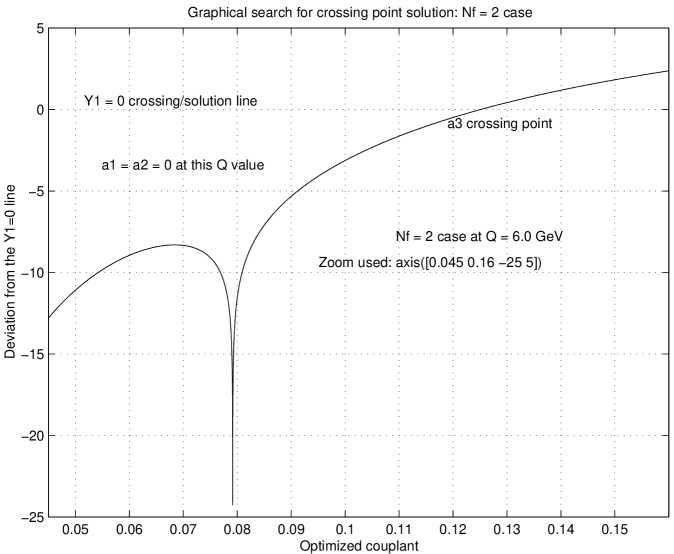
Figure 1: Sample crossing point profile on the Y1 = 0 line, Nf = 2 case

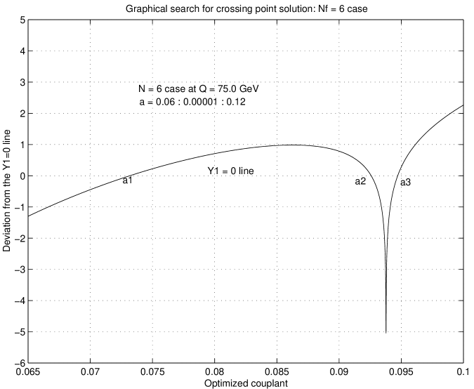
Figure 2: Sample crossing point profile on the Y1 = 0 line, Nf = 6 case

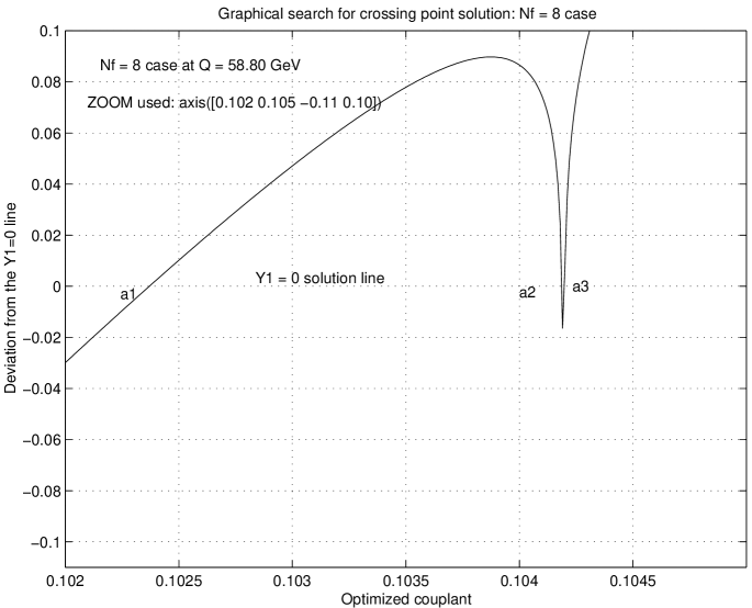
Figure 3: Sample triple point crossing profile on the Y1 = 0 line, Nf = 8 case

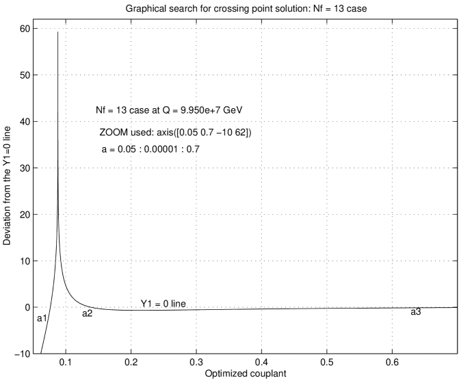
Figure 4: Sample crossing point profile on the Y1 = 0 line, Nf = 13 case

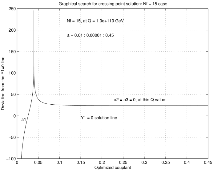
Figure 5: Sample crossing point profile on the Y1 = 0 line, Nf = 15 case

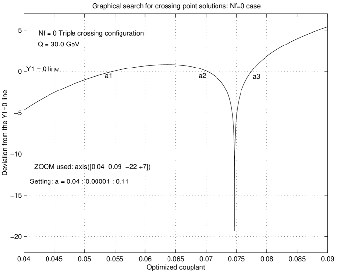
Figure 6: Triple point crossing configuration on the Y1 = 0 line, Nf = 0 case

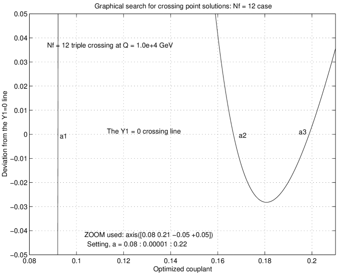
Figure 7: Sample (triple) point crossing profile on the Y1 = 0 line, Nf = 12 case

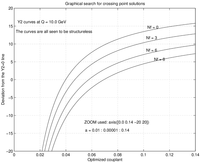
Figure 8: Crossing point profiles on the Y2 = 0 line

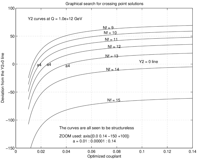
Figure 9: Crossing point profiles on the Y2 = 0 line

A simple MATLAB program we used for plotting out these $(Y_{1}(a),a)$, and $(Y_{2}(a),a)$ curves, and reading off the crossing point values of $a$, on the couplant axis, is reproduced as Appendix A. The crossing point readings from the $(Y_{1}(a),a)$ plot, being solutions of eqn. (56), we have called the $Y_{1}$ component of Padé QCD. Similarly, we can call the crossing point readings from the $(Y_{2}(a),a)$ plot, being solutions of eqn. (57), the $Y_{2}$ component of Padé QCD. We find that the two solutions or components of Padé QCD are in general different and distinct from each other, implying immediately, that the $[1|1]$ optimized Padé QCD couplant has at least two separate components (solutions), we shall from here onwards refer to as the $Y_{1}$ and $Y_{2}$ component couplants of Padé QCD.

4 FEATURES FOUND IN THE $[1|1]$ OPTIMIZED PADÉ COUPLANT EQUATION

We now state the features we found with the above graphical and computational analysis of the optimized $[1|1]$ Padé QCD couplant eqn. (55). Later we point out which of these features persist as intrinsic features of the other Padé QCDs we also analysed by the same graphical method.

4.1 The Multiplicity Structure in the $Y_{1}$ Padé Component Solution

One striking feature we found in the course of studying the above $(Y_{1}(a),a)$, and $(Y_{2}(a),a)$ Padé QCD plots, is that while the $(Y_{2}(a),a)$ plot is simple and structureless for all flavor numbers $N_{f}$, eqn. (56) and its $(Y_{1}(a),a)$ plots have in general three different but simultaneous crossing points on the couplant axis, for a given Q value, implying that eqn. (56) has in general three different solutions for the same Q value and the same flavor number, and this feature holds for each flavor number : $0\leq N_{f}\leq 16$. Typical such (simultaneous) triple crossing points can be seen in figs. 2 to 7. The feature exists for every flavor number $0\leq N_{f}\leq 16$.

The first graphical indication of the existence of this triple multiplicity solution of eqn. (56) is the observation that as Q increases from below, the entire profile of the $(Y_{1}(a),a)$ plot rises upwards, such that beginning with the plot (at low Q) cutting the couplant axis at only one distant point to the far right hand side of the couplant axis, the curve later rises enough (at higher Q values) to begin to cut and cross the couplant axis simultaneously at three distinct points. We found that this begins to occur when Q has attained a certain minimum or threshold value we have denoted by $Q_{\mathrm{min}}$, and that this minimum Q value exists as a sharply defined threshold point for each flavor number $N_{f}$ . Significantly however, the actual value of $Q_{\mathrm{min}}$, (see Table 2), differed from one flavor number system to another. These rising profiles of the $(Y_{1}(a),a)$ plots and their triple crossings for $Q\geq Q_{\mathrm{min}}$ are shown in figs. 10 to 14 for some flavor numbers, the pattern being however the same for all flavor numbers. Figures 15 to 18 show sample profile positions when one is at exactly the threshold (critical) point $Q=Q_{\mathrm{min}}$ for these rising profiles.

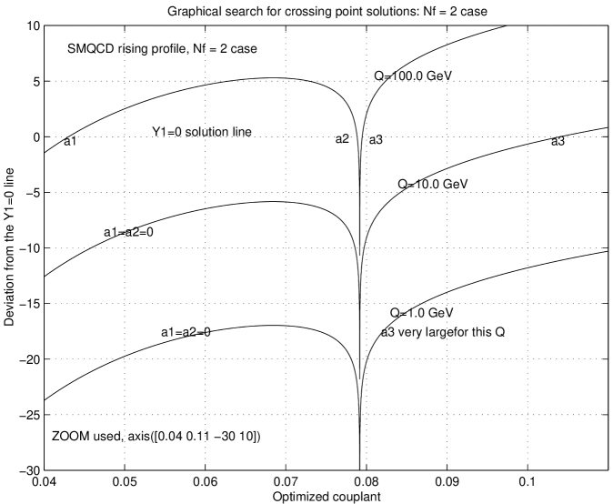
Figure 10: Y1 rising profiles, Nf = 2 case

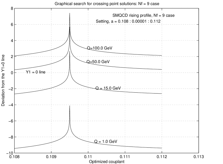
Figure 11: Y1 rising profiles, Nf = 9 case

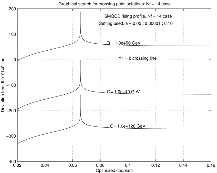
Figure 12: Y1 rising profiles, Nf = 14 case

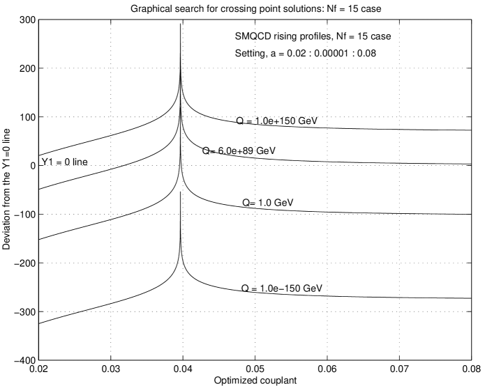
Figure 13: Y1 rising profiles, Nf = 15 case

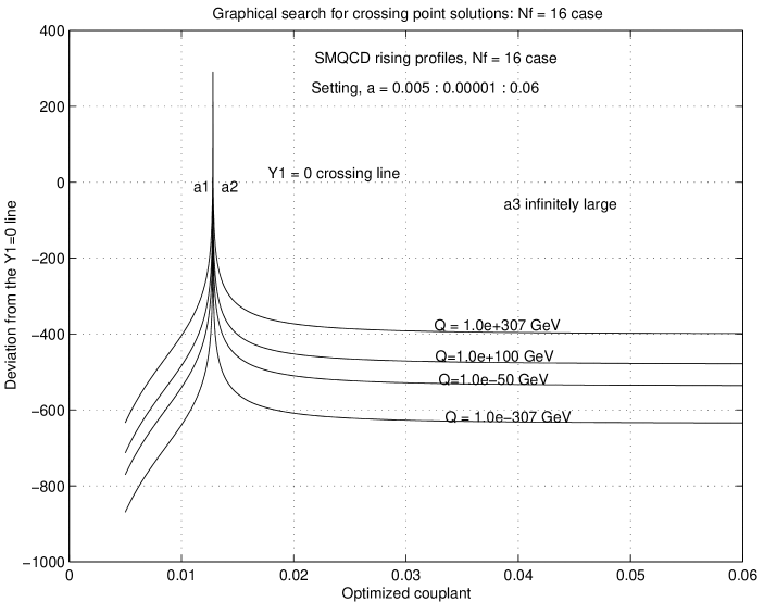
Figure 14: Y1 rising profiles, Nf = 16 case

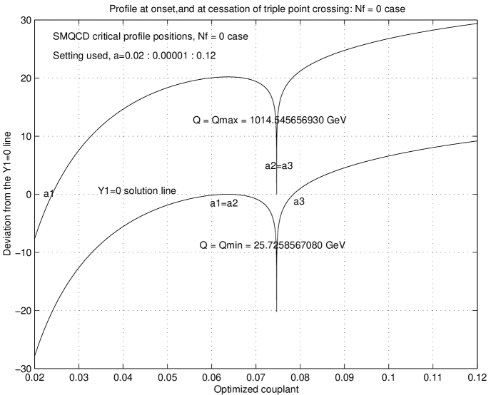
Figure 15: Critical momentum profile configurations on the Y1 = 0 line, Nf = 0 case

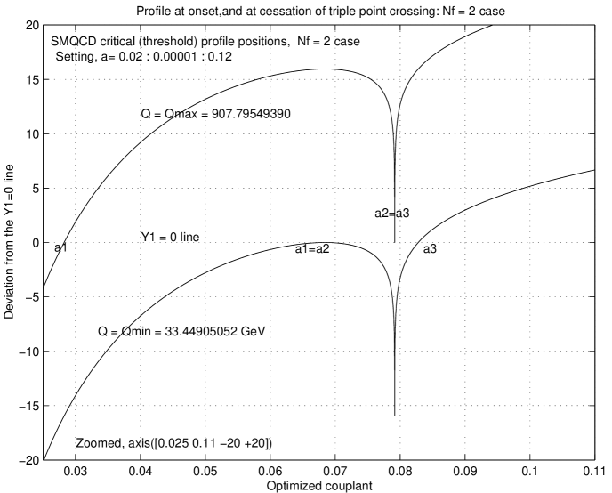
Figure 16: Critical momentum profile configurations on the Y1 = 0 line, Nf = 2 case

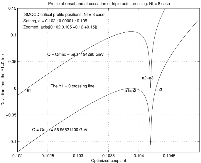
Figure 17: Critical momentum profile configurations on the Y1 = 0 line, Nf = 8 case

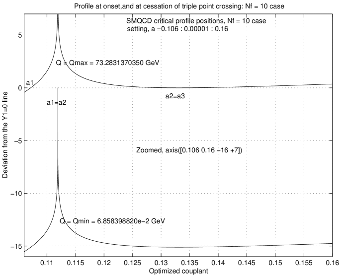
Figure 18: Critical momentum profile configurations on the Y1 = 0 line, Nf = 10 case

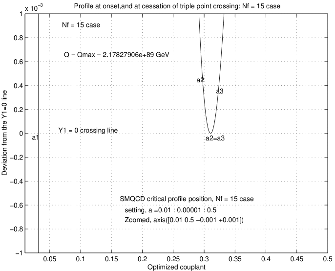
Figure 19: Critical momentum profile configurations on the Y1 = 0 line, Nf = 15 case

We observed also from the same $(Y_{1}(a),a)$ profile plots that the triple crossing point feature does not persist for all $Q\geq Q_{\mathrm{min}}$. Rather, as Q rises higher and higher above $Q_{\mathrm{min}}$, the triple crossing suddenly ceases and we noted that this occurs when Q has attained some upper cut-off value we denoted by $Q=Q_{\mathrm{max}}$. This upper cut off value of Q was found to be as precise and sharply defined for each $N_{f}$ flavor system as the lower threshold point $Q=Q_{\mathrm{min}}$. But, again as in the $Q_{\mathrm{min}}$ case, the value of $Q_{\mathrm{max}}$, (see Table 2), differed from one $N_{f}$ flavor system to another. The upper parts of Figures 15 to 19 show sample profiles and configurations at the cessation point of triple crossings when $Q=Q_{\mathrm{max}}$.

By way of comparison, we show in figs. 20 to 22 the profiles of the $(Y_{2}(a),a)$ plots for some flavor numbers. None of these has a triple crossing structure, but only one solution or crossing point for eqn. (57) at any one value of Q, and for all flavor numbers.

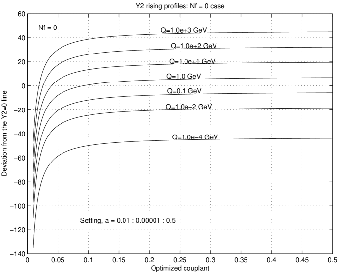
Figure 20: Y2 rising profiles, Nf = 0 case

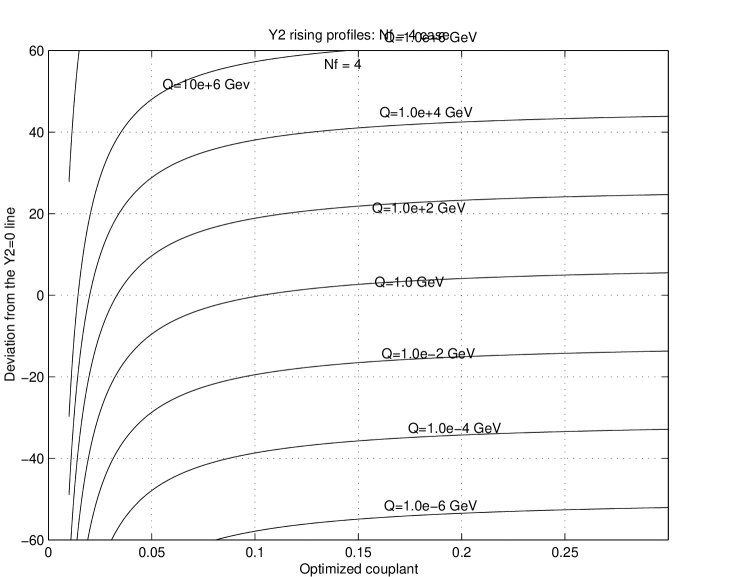
Figure 21: Y2 rising profiles, Nf = 4 case

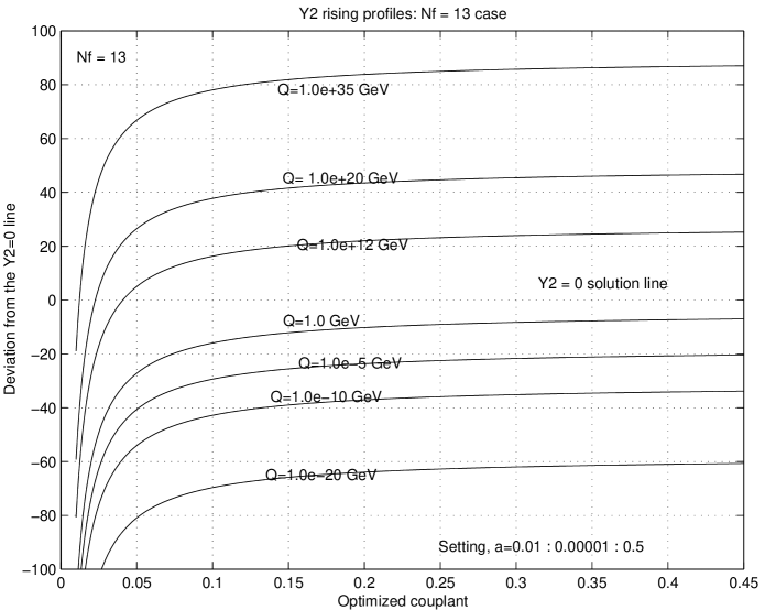
Figure 22: Y2 rising profiles, Nf = 13 case

Focusing now on these crossing point solutions of eqns. (56) and (57), we can denote by $a_{1},a_{2},a_{3}$, the general triple point crossing solutions of eqn. (56), and by $a_{4}$ the one solution (crossing point) of eqn. (57). Here $a_{1}$ is the extreme left crossing point in the $(Y_{1}(a),a)$ plot, $a_{2}$, is the middle crossing point, while $a_{3}$, is the extreme right crossing point, all in the same $(Y_{1}(a),a)$ plot of any given (fixed) $N_{f}$ system. Together the four solutions $a_{1},a_{2},a_{3},a_{4}$ imply that the Padé approximant QCD couplant $a$ of eqn. (55) or eqn. (1), has a multiplicity structure of four distinct component couplants or color force solutions, we can read off as crossing points on our Y1 = 0 and Y2 = 0 solution lines. This multiplicity of solutions of the Padé couplant equation (55), exhibited in the momentum band $Q_{\mathrm{min}}\leq Q\leq Q_{\mathrm{max}}$, represents our first explicit finding concerning the features of Padé QCD couplant analyzed by our above computational and graphical method.

4.2 Features of the $a_{1}(Y_{1}),a_{2}(Y_{1}),a_{3}(Y_{1})$, and $a_{4}(Y_{2})$ Padé couplant Solutions.

We investigated next the behavior of each Padé component couplant solution, by plotting its graphical Padé crossing point values against the momentum Q of the profile plot at which the crossing point value was read off. We found the following features.

4.2.1 Features of the $a_{3}$ Padé component couplant solution

From fig. 1 we see that the $a_{3}$ is the only solution or crossing point of eqn. (56) in the low energy momentum region $Q<Q_{\mathrm{min}}$, and for any given flavor number $N_{f}$, particularly in the range, $0\leq N_{f}\leq 8$. For $9\leq N_{f}\leq 16$, the indication from figs. 11 to 14 as well as figs. 38 , 40 and 42, is that the $a_{3}$ is already infinitely large even before we reach the point $Q=Q_{\mathrm{min}}$. If we combine this with the features of the $a_{3}$ shown in fig. 23 for the $0\leq N_{f}\leq 8$ cases, the indication is that while the $a_{3}$ does exist in general in the region $Q<Q_{\mathrm{min}}$, it has the form of a Landau type pole singularity for a Padé beta function or couplant. This is re-inforced by the fact seen in fig. 23 that even for the lowest $N_{f}=0$ case, the $a_{3}$ already rises sharply towards very large values at $Q=0.705$ GeV, in the process still cutting off access into the infra-red region $Q<0.705$ Gev.

The $a_{3}$ exists in the medium energy region $Q_{\mathrm{min}}\leq Q\leq Q_{\mathrm{max}}$ but with a value that decreases progressively with increasing momentumQ. It finally cuts off at the characteristic higher momentum $Q=Q_{\mathrm{max}}$ such that for all $Q>Q_{\mathrm{max}}$, $a_{3}=0$. Because this second Padé couplant bifurcation point occurs well inside the normal PQCD region of QCD, $Q\geq\Lambda_{\mathrm{QCD}}$, with $Q_{\mathrm{max}}\gg\Lambda_{\mathrm{QCD}}$, the possibility arises that if the above Padé couplant structure represents physical QCD reality, the Padé $(a_{3},a_{2})$ structure can affect substantially even relatively high energy QCD processes, by way of distinctively non-perturbative contributions.

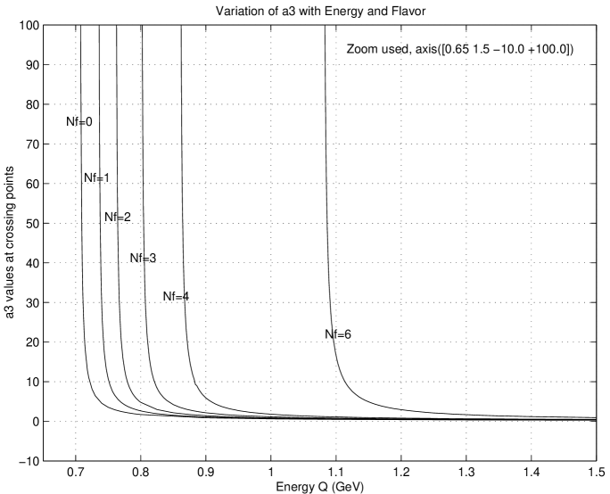
Figure 23: Pattern of variation with momentum and flavor, of isolated Padé $a_{3}$ component color force solution

4.2.2 Features of the $a_{1}$ Padé component couplant solution

Examining the $a_{1}$ Padé component couplant solution in the same way, we observe from fig. 5 as well as the upper halfs of figs. 15 to 19, that the $a_{1}$ solution (crossing point) is the only Padé QCD present in the very high energy region $Q>Q_{\mathrm{max}}$ where it also has very small values for any flavor number, such that for $Q\rightarrow\infty$, $a_{1}\rightarrow 0$, shown in fig. 24.

The $a_{1}$ couplant solution exists in the intermediate energy region: $Q_{\mathrm{min}}\leq Q\leq Q_{\mathrm{max}}$ attaining its highest but still moderate value at $Q=Q_{\mathrm{min}}$ from where it decreases progressively towards zero as $Q\rightarrow\infty$. The $a_{1}$ solution does not exist in the low energy region $0\leq Q<Q_{\mathrm{min}}$.

The indication from these features is that the Padé $a_{1}$ component solution can be identified as the asymptotically free purely PQCD component color force of QCD we started with in eqns. (1) and (9). We shall so identify the $a_{1}$ component Padé solution. Then the fact that the $a_{1}$ solution does not exist in the region $0\leq Q<Q_{\mathrm{min}}$ is seen as a correct reflection of the denominator zero singularity of the Padé beta function eqn. (20) and its attendant Kogan-Shifman [3] type behavior, with our $Q_{\mathrm{min}}$ directly identifiable with the $\mu_{c}$ cut off momentum of Kogan and Shifman, and of Elias et. al. [1, 2].

Based on these identifications, the question of whether infra-red scenario I (frozen couplant), or scenario II (bifurcated infra-red attractor point) holds at any flavor in Padé QCD and perhaps in real QCD, boils down in our approach to the question of the extent the momentum gap $0\leq Q<Q_{\mathrm{min}}$ remains finite and free of our $(a_{1},a_{2})$ bifurcating components, in various flavor states of QCD. We will find that our method allows us to answer this question explicitly later.

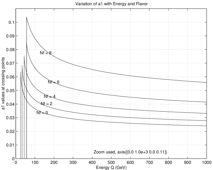
Figure 24: Pattern of variation with momentum and flavor, of isolated Padé $a_{1}$ component couplant solution

4.2.3 The $a_{2}$ Padé component couplant solution

Plotting the $a_{2}$ crossing point values against momentum Q, we find the behavior shown in fig. 25. That is, the $a_{2}$ component color force solution is found to exist only in the intermediate energy region $Q_{\mathrm{min}}\leq Q\leq Q_{\mathrm{max}}$ for any flavor number $N_{f}$, but vanishes or cuts off sharply at the two critical upper and lower momentum points $Q=Q_{\mathrm{max}}$ and $Q=Q_{\mathrm{min}}$.

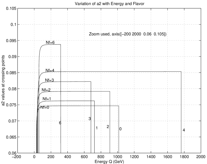
Figure 25: Pattern of variation with momentum and flavor, of isolated Padè $a_{2}$ component couplant solution

From fig 25, we see that inside its intermediate energy domain of operation and existence, the $a_{2}$ couplant rises in value from a lowest value at $Q=Q_{\mathrm{min}}$ to a highest value at $Q=Q_{\mathrm{max}}$. This manner of behavior suggests we identify our Padé $a_{2}$ component with the upper branch of the bifurcated structure found by Elias et. al. [1, 2] and by Kogan and Shifman [3]. This is reinforced by the observation from our profile plots shown variously in figs. 1 to 19 that the $a_{2}$ crossing point solution merges with and coincides exactly in value with the $a_{1}$ couplant solution at the point $Q=Q_{\mathrm{min}}$ which can be regarded as a bifurcation point of the $a_{1}$ into $a_{2}$. Then the infra-red region $0\leq Q<Q_{\mathrm{min}}$, is totally free of the two bifurcated component couplants, $a_{1}$ and $a_{2}$, again agreeing fully with the behavior found by Elias et. al. [1, 2], and by Kogan-Shifman [3].

However, unlike the Elias et. al. structure which did not determine the progression of this $a_{2}$ upper branch, our graphical crossing point solution method shows the $a_{2}$ clearly as terminating and merging exactly with the $a_{3}$ crossing point solution at the point $Q=Q_{\mathrm{max}}$, where $a_{2}=a_{3}$, and both couplants thereafter disappear together for all $Q>Q_{\mathrm{max}}$. One may say that the $a_{2}$ bifurcates further into the $a_{3}$ which then runs towards the infra-red region but soon rises sharply to very large values in a manner suggestive of a Landau pole behavior. This $a_{3}$ presence was not discernible from the numerator and denominator zero analysis of Elias et. al. [1, 2].

4.2.4 The $a_{4}(Y_{2})$ Padé component couplant solution

The $a_{4}(Y_{2})$ crossing point solution, arose from the separate eqn. (57). As such it emerges for now as a lone star Padé component color force, not connected to the $a_{1},a_{2},a_{3}$ components of eqn. (56). Its features are shown in fig. 26, where it is seen that it has no structure or bifurcation but behaves smoothly, falling asymptotically in value from a large value $(a_{4}\rightarrow\infty)$ near $Q\rightarrow 0$, to the value $(a_{4}\rightarrow 0)$ as $(Q\rightarrow\infty)$. The exact meaning of the $a_{4}$ couplant solution is not yet clear to us, and is being investigated.

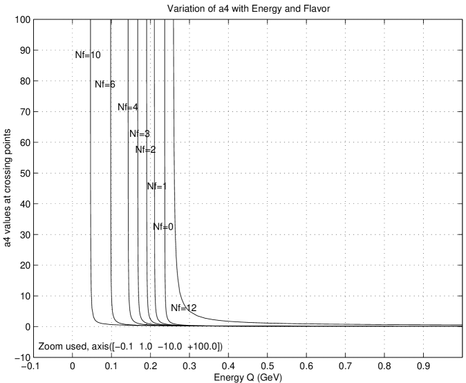
Figure 26: Pattern of variation with momentum and flavor of Padé $a_{4}$ component couplant solution

4.3 Spiral Chain-like Structure found in Padé QCD

Arising from the fact stated above that while the $a_{1},a_{2},a_{3}$ are independent solutions of Padé eqn. (56), they are however joined together at the two critical (bifurcation) momentum points $Q_{\mathrm{min}}$ and $Q_{\mathrm{max}}$, in the manner given by:

$$a_{1}=a_{2}\neq 0,\mathrm{at}:Q=Q_{\mathrm{min}},$$

and

$$a_{2}=a_{3}\neq 0,\mathrm{at}:Q=Q_{\mathrm{max}}.$$

we find that a combined plot of the individual variations $(a_{1},Q);(a_{2},Q);(a_{3},Q)$ gives one unbroken chain-like spiral structure, shown in figs. 27 to 43 for various flavors. The $a_{4}$ component has also been plotted in.

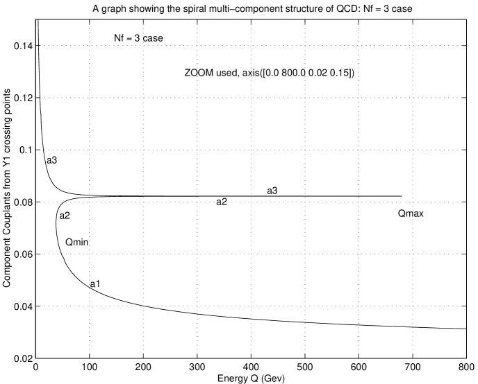
Figure 27: A plot showing a spiral multi-component structure of Padé QCD: Nf = 3 case

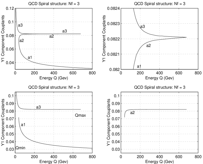
Figure 28: A plot showing a multi-component couplant structure in Padé QCD: Nf = 3 case

These chain-like spiral structures together with our computed values of the bifurcation point critical momenta $Q_{\mathrm{min}}$ and $Q_{\mathrm{maxc}}$ shown in Table 2, lead us to explicitly answer the question, for which flavor states the infra-red scenario I or scenario II holds. Additionally, we have also shown in Table 2, the values of the Padé couplants $a_{1}(Q_{\mathrm{min}})$ and $a_{3}(Q_{\mathrm{max}})$ at these critical cut-off momentum points. They all enable us to answer the same question definitively. Before discussing the question however, we first show that the above features of the optimized $[1|1]$ Padé QCD are also shared to a large extent by the other Padé QCDs, $[1|1]$, $[2|1]$ and $[1|2]$ that we also analyzed.

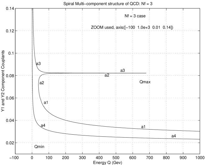
Figure 29: A plot showing a spiral multi-component structure in Padé QCD: Nf = 3 case

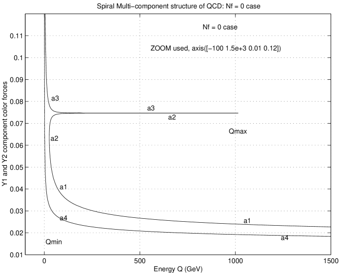
Figure 30: A plot showing a spiral multi-component structure in Padé QCD: Nf = 0 case

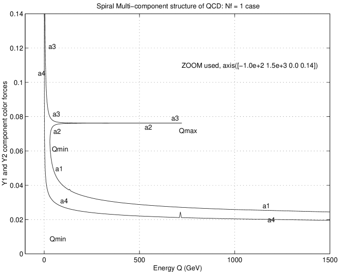
Figure 31: A plot showing a spiral multi-component structure in Padé QCD: Nf = 1 case

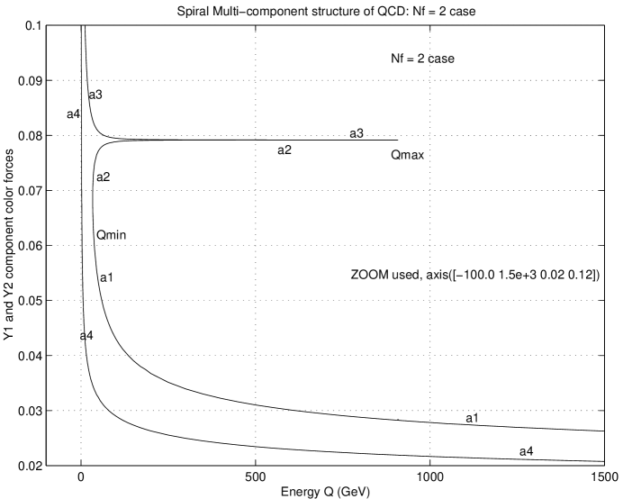
Figure 32: A plot showing a spiral multi-component structure in Padé QCD: Nf = 2 case

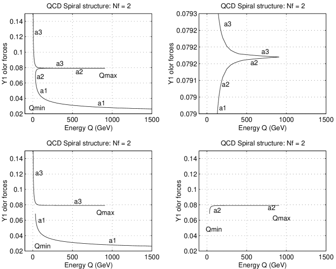
Figure 33: A plot showing a multi-component couplant structure in Padé QCD: Nf = 2 case

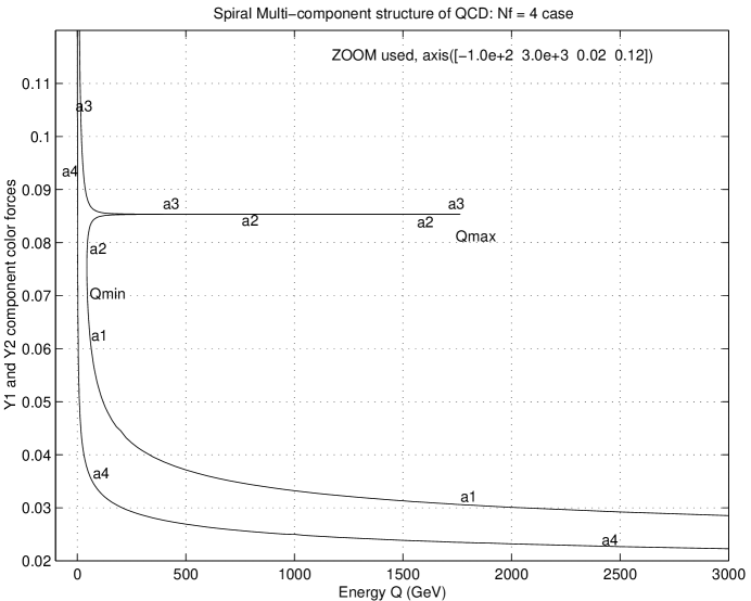
Figure 34: A plot showing a spiral multi-component structure in Padé QCD: Nf = 4 case

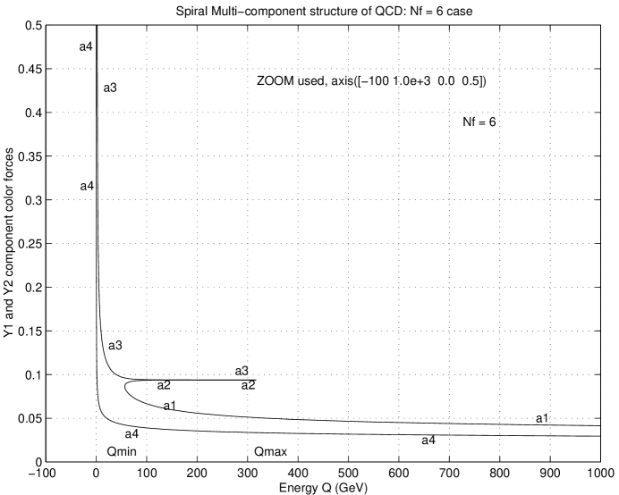
Figure 35: A plot showing a spiral multi-component structure in Padé QCD: Nf = 6 case

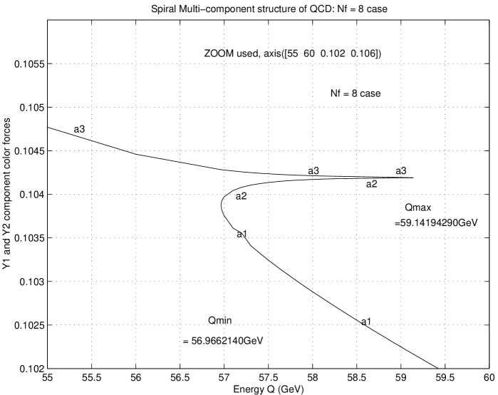
Figure 36: A plot showing a spiral multi-component structure in Padé QCD: Nf = 8 case

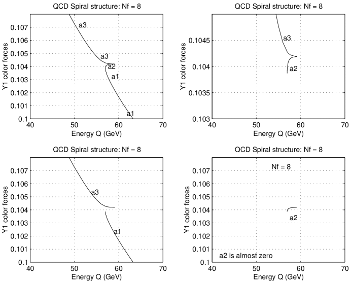
Figure 37: A plot showing a multi-component couplant structure of Padé QCD: Nf = 8 case

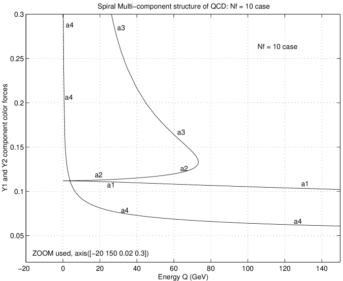
Figure 38: A plot showing a spiral multi-component structure in Padé QCD: Nf = 10 case

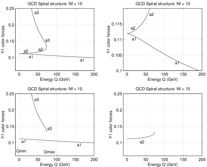
Figure 39: A plot showing a multi-component couplant structure in Padé QCD: Nf = 10 case

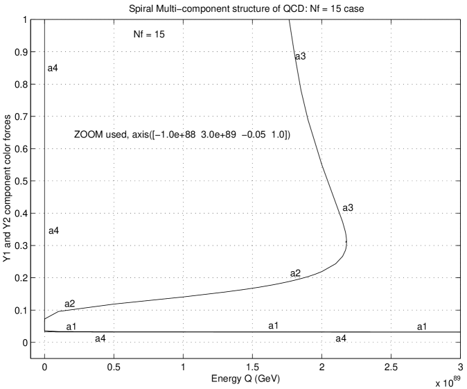
Figure 40: A plot showing a spiral multi-component structure in Padé QCD: Nf = 15 case

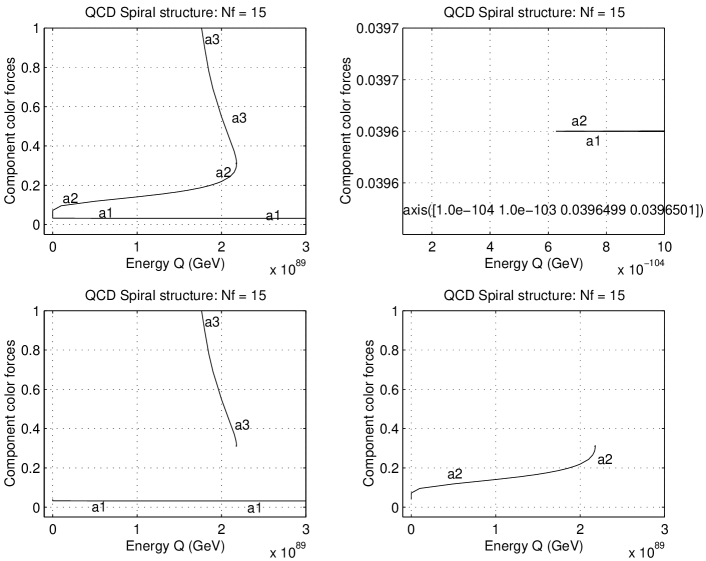
Figure 41: A plot showing a multi-component couplant structure of Padé QCD: Nf = 15 case

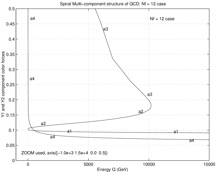
Figure 42: A plot showing a spiral multi-component structure in Padé QCD: Nf = 12 case

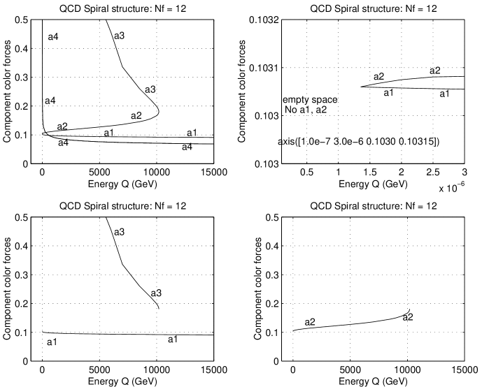
Figure 43: A plot showing a multi-component couplant structure of Padé QCD: Nf = 12 case

5 ANALYSIS AND FEATURES OF THE NON-OPTIMIZED $[1|1],[2|1]$ AND $[1|2]$ PADÉ QCDs

. Using exactly the same computational and graphical procedures described above for the optimized $[1|1]$ Padé QCD, we also analyzed the non-optimized $[1|1],[2|1]$, and $[1|2]$ Padé QCD couplant equations (25) , (28) and (31). We found essentially the same Padé QCD features, with small differences which we summarize as follows.

1. The $a_{4}$ component solution found in optimized Padé QCD is not exhibited by any of the three non-optimized Padé QCDs. As will be recalled, the $a_{4}$ solution arose from the quadratic nature of the optimized $c_{2}$ coefficient given in eqns. (49) and (50). This $c_{2}$ quadratic feature is not present in the non-optimized $[1|1],[2|1],[1|2]$ Padé QCDs, and as such the $a_{4}$ solution does not arise in these cases. We can therefore for the moment play down the existence and role of the Padé $a_{4}$ component solution.

2. However, the triple crossing point feature and hence the $a_{1},a_{2},a_{3}$ component structure, are present in exactly the same form in all the four Padé QCDs we analyzed, optimized or not. Correspondingly, the spiral chain-like structure exists in all of them and can be taken as intrinsic characteristic feature of a Padé QCD.

3. We found that while each Padé QCD at a given flavor, is characterized by two critical or cut off momenta $Q_{\mathrm{min}}$ and $Q_{\mathrm{max}}$, the actual values of these momentum pairs differed substantially from one Padé QCD to other. The values found for example, for the non-optimized $[1|1]$ Padé QCD are shown in Table 3 to be compared with Table 2 for the optimized $[1|1]$ Padé QCD. The $[2|1]$ and $[1|2]$ paired critical momenta differ just as much. The trend of the variation is not yet clear but is being separately studied.

4. In contrast, the values of the critical (cut-off) couplants $a_{1}(Q_{\mathrm{min}})$ and $a_{3}(Q_{\mathrm{max}})$ exhibit some consistency, especially in high flavor states seen in Tables 2 and 3.

5. We found that the optimized $[1|1]$ Padé QCD has the feature of resolving clearly, the spiral nature of the $N_{f}=6,7,8$ flavor states shown in figs. 35 and 36, compared to the non-optimized $[1|1]$ Padé QCD where the couplant structure of the same $N_{f}=6,7,8$ flavor states, is not so resolved, as can be seen in fig. 44.

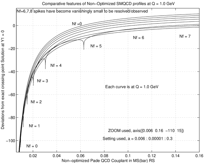
Figure 44: Combined Profile features of Non-optimized $[1|1]$ Padé QCD at Q = 1.0 GeV, for $0\leq N_{f}\leq 8$

.

The above small differences apart, we affirm that our Padé QCD of various orders, optimized or not, has the characteristic feature of triple multiplicity of solutions $(a_{1},a_{2}.a_{3})$; two characteristic bifurcation points, $Q_{\mathrm{min}}$ and $Q_{\mathrm{max}}$; and a spiral chain-like structure continuously connecting the three component solutions, $(a_{1},a_{2},a_{3})$. Using figs. 27 to 43 of the $[1|1]$ NNLO optimized Padé QCD as typical of these behaviors and properties of a Padé QCD, we now consider the question of which of infra-red scenario I or II holds at a given flavor.

6 THE QUESTION OF IR SCENARIO I OR SCENARIO II IN PADÉ QCD

As already stated, in our approach, the question of whether we have infra-red scenario I (IR stable fixed point and frozen couplant) or IR scenario II (IR attractor point and bifurcated couplant) is directly decided by whether the momentum gap $0\leq Q<Q_{\mathrm{min}}$ exists and is finite. Where this is the case, the IR scenario II necessarily holds, ruling out scenario I. Conversely, if the momentum gap does not exist for a given flavor, the IR structure of that flavor state is necessarily of scenario I type, and scenario II becomes ruled out. We now examine our spiral plots as well as our Table 2 to see which scenario holds. We find as follows:

1. The case $0\leq N_{f}\leq 5$
   From our spiral plots figs. 27 to 34 it is clear that IR scenario II is what operates and not scenario I. The same conclusion is drawn from our Tables 2 and 3, where it is seen that the momentum gap $0\leq Q\leq Q_{\mathrm{min}}$ is far from being zero. These findings agree with those of Elias et. al. who found that scenario II holds for all $0\leq N_{f}\leq 5$, regardless of which Padé approximants, $[1|2],[2|1],[1|3],[3|1]$, or $[2|2]$ they used.

2. The case $N_{f}=6,7,8$
   From our spiral plots shown in figs. 35 and 36 it is also clear that IR scenario II holds for $N_{f}=6,7,8$, and not scenario I. The $Q_{\mathrm{min}}$ values shown in Tables 2 confirm this further. The momentum gap $0\leq Q\leq Q_{\mathrm{min}}$ is far from being zero in all these cases.

3. The case $9\leq N_{f}\leq 16$
   For these flavor states, Elias et. al. by their method, found scenario I IR behavior. In contrast, our method shows the opposite scenario II behavior for all $9\leq N_{f}\leq 16$ as for all $0\leq N_{f}\leq 8$. Our finding of scenario II for all $9\leq N_{f}\leq 16$ is seen clearly in figs. 38 to 43 for the cases of $N_{f}=10,12,15$, chosen for illustration. All the other flavor states $N_{f}=9,11,13,14.16$, have exactly the same scenario II behavior.

   We can explain this particular difference in the two results, and establish that our finding is the correct Padé position. Looking at figs. 38 to 43 as well as Tables 2 and 3, it is seen that the infra-red attractor points exist at progressively lower and lower momentum in these high flavor states, and only a method designed to follow this trend can establish the continued existence of the scenario II behavior. The Elias et. al. method would appear not equipped for this.

   Even with our method, looking only at our figs. 38, 40, and 42, one would gain the impression that our $a_{1}$ and $a_{2}$ Padé component couplants which are the exact analogue of Elias et. al. bifurcated couplants at $\mu=\mu_{c}$, stretch on to zero momentum point, $Q=\mu=0$ in which case scenario I could be concluded.

   However, if one follows these two branch Padé component couplants $a_{1}$ and $a_{2}$, to sufficiently low momentum regions, shown typically in our figs. 41 and 43, one sees unambiguously, that these two component couplants still meet and turn back at some finite critical momentum $Q_{\mathrm{min}}=\mu_{c}\neq 0$, leaving a clearly visible gap, $0\leq Q<Q_{\mathrm{min}}$, where both the $a_{1}$ and $a_{2}$ are totally absent. This gap is present and completely visible in all cases $9\leq N_{f}\leq 16$, leaving no doubt that scenario II is intrinsically what holds in these Padé flavor cases as for the $0\leq N_{f}\leq 8$ cases.

   It just happens that for the higher flavor states, the spiral (bifurcation) point where $a_{1}$ and $a_{2}$ meet, shifts to lower and lower momentum point, and unless this shifting is followed from flavor to flavor, one can conclude erroneously that scenario I operates in these higher flavor states.

Against the above, we can affirm that our results are actually consistent with those of Elias et. al. and that the features we found and analyzed in our Padé QCDs, are the intrinsic features of Padé QCD of any order $[1|1],[2|1],[1|2],[3|1],[1|3]$ or $[2|2]$. However our graphical method of analyzing these Padé QCD features, has the advantage of showing clearly that the infra-red scenario II behavior is the intrinsic behavior of Padé QCD in all flavor states $0\leq N_{f}\leq 16$, and not IR scenario I.

We are led also to firmly identify our critical momentum point $Q_{\mathrm{min}}\equiv\mu_{c}$ as fundamentally an infra-red attractor point or a pole singularity of Padé QCD beta function, for all flavor states, $0\leq N_{f}\leq 16$. This means that the critical Padé QCD couplants $a_{1}(Q_{\mathrm{min}})$ shown in Table 2 are fundamentally infra-red attractor points and not IR stable fixed points, although for sufficiently high flavor $N_{f}$, the attractor behavior (point) can be mistaken for a IR stable fixed point or frozen couplant behavior.

7 COMPARISON WITH TRUNCATED PQCD INFRA-RED FIXED POINT RESULTS

Having settled the above question, we can check for further consistency of our Padé QCD compuatations and findings by comparing them with the earlier work of Banks and Zaks [6]; and of Stevenson et. al. [4, 5, 7, 8], who used purely truncated PQCD beta function to search for infra-red (IR) fixed points in PQCD. Banks and Zaks [6] as well as Stevenson [7] analyzed the NLO truncated PQCD of eqn. (8) and predicted PQCD IR fixed points shown against flavor numbers in our Table 4. Separatelyly, Stevenson et. al. [4, 5, 7, 8], using optimized NNLO truncated PQCD of eqn. (9) investigated the same IR fixed point structure of PQCD. The IR fixed points they found are shown in the same Table 4. We can now compare these results with our $a_{1}$ values computed from our $[1|1]$ optimized (NNLO) Padé QCD. These $a_{1}(Q_{\mathrm{min}})$ values are also shown side by side in Table 4. We now observe as follows.

1. For low flavors $N_{f}$, there is no agreememt between our $a_{1}$ values and the NLO or NNLO IR fixed point values of the above authors. This is consistent with the earlier stated fact that the point $(Q_{\mathrm{min}},a_{1}(Q_{\mathrm{min}}))$ is not an IR stable fixed point of QCD but a pole singularity (IR attractor point) of the beta function.

2. For very high $N_{f}=16,15,14,13..$, our values of $a_{1}$ agree almost exactly with the NLO and NNLO IR stable fixed point values of the above authors. This agreement is evidence that our Padé QCD computations and graphical solution method are correct and reliable. However, the agreement comes not because our $a_{1}(Q_{\mathrm{min}})$ point has suddenly become IR stable fixed point of scenario I, but from the spiral structure shifting to lower and lower momentum points discussed earlier. As a result of this shifting, the IR attractor point $a_{1}(Q_{\mathrm{min}})$ becomes mimiced more and more effectively by an IR stable fixed point of a seemingly frozen PQCD (or $a_{1}$) couplant. But when one follows this bifurcation point shifting to sufficiently low energy as shown typically in our figs. 41 and 43, one soon sees that $a_{1}$ and $a_{2}$ are still separate or bifurcated component couplants and that the PQCD couplant $a_{1}$ did not freeze at all.

We conclude finally that our Padé QCD graphical computations and findings, can be relied upon, being consistent with the independent Padé beta function numerator/denominator zero analysis of Elias et. al.; and also consistent with the direct PQCD IR computations of Banks and Zaks, and Stevenson et. al.

8 SUMMARY AND CONCLUSIONS

We have presented a reliable and consistent graphical computational method of analyzing the infra-red structure of Padé approximant QCDs. We have shown with the method that the intrinsic behavior of Padé QCD is one in the PQCD bifurcates at some critical Kogan-Shifman type momentum $\mu_{c}=Q_{\mathrm{min}}$, leaving the infra-red region $0\leq\mu<\mu_{c}$ totally decoupled from the PQCD dynamics. We found however that besides this PQCD bifurcation, there exists a second bifurcation by the upper branch $a_{2}$ couplant, into a third branch or component couplant $a_{3}$, at another critical momentum $Q_{\mathrm{max}}$ where in all cases, $Q_{\mathrm{max}}>Q_{\mathrm{min}}$. The three components or branches $(a_{1},a_{2},a_{3})$ are arranged in a chain-like spiral structure. The $a_{3}$ in general runs into the original infra-red region $\mu<\mu_{c}$ but soon rises sharply to very large values in a manner suggestive of a Landau pole behavior of the Padé couplant at its second bifurcation point. The extent to which the above Padé QCD features and structure can be taken over as those of real physical QCD is a matter for further studies which we are now following up.

Acknowledgements The author is grateful to Dr. Billy Bonner, Director T.W. Bonner Nuclear Laboratory, Rice University, for providing him office space in the laboratory and for general hospitality. He thanks Dr. P. M. Stevenson, Professor of Physics at the same Laboratory for discussion concerning his optimization principle used in this paper. The author thanks Dr. V. Elias for reading through an earlier version of this paper, and making useful comments. Some computing assistance received from Niki Serakiotou and Pablo Yepes is gratefully acknowledged. The work would however never have been possible neither would the author’s visiting stay at Rice University, without the sustained financial support made available to the author from outside sources. He thanks all contributors. The author is particularly grateful to Dr. Awele Ndili of Stanford University, California, who provided him a lot of technical advice with regard to computing and software, and specifically purchased a modern PC for the author‘s use, on which all the computations and figures reported in this paper were done.

Appendix A (Appendix A): The exact MATLAB Program (QCD3.m) used by the author to solve numerically, the optimized SMQCD eqn. (55) of this paper

% The footnotes given below are to guide the actual execution of the program; they are not part of the program.
% The program now begins.

clear all;
$N=2$; % see footnote No. 1 below.
Rh2 = -10.91120013471925; % see footnote No. 2 below.
$Q=1.0;$ % see footnote No. 3 below.
$L=0.230;$ % L = $\Lambda_{\mathrm{QCD}}=0.230$ GeV, kept constant all through the SMQCD computations.
$r1=1.9857-0.1153*N;$ % $r1$ is a constant all through the (optimized) SMQCD computations.
$b=(33-2*N)/6;$ % $b$ is a constant all through the SMQCD computations.
$c=(153-19*N)/(66-4*N);$ % $c$ is a constant all through the SMQCD computations.
Rh1 = $b*log(Q/L)+c*log(2*c/b)-r1;$ % see footnote No. 4 below.
$D=8*c*c-4*Rh2;$ % $D$ varies as we vary input Rh2.
$P1=3*c/2+sqrt(D)/2;$ % $P1$ varies as we vary input Rh2.
$P2=3*c/2-sqrt(D)/2;$ % $P2$ varies as we vary input Rh2.
X1 = Rh1 - P1; % X1 varies as we vary Q and Rh2.
X2 = Rh1 - P2; % X2 varies as we vary Q and Rh2.
$a=0.02:0.00001:0.12;$ % see footnote No. 5 below.
$F1=1.0+c*a-2*a*P1;$ % $F1$ is just a notation.
$F2=1.0+c*a-2*a*P2;$ % $F2$ is just a notation.
$H1=((c*a)./F1);$ % note the space and the dot before /F1
$H2=((c*a)./F2);$ % note the space and the dot before /F2
$X3=(1./a)+c*log(abs(H1));$ % note the space and the dot before /a
$X4=(1./a)+c*log(abs(H2));$ % note the space and the dot before /a
Y1 = X1 - X3;
Y2 = X2 - X4;

plot(a, Y1); grid on % see footnote No. 6 below.
xlabel(‘Optimized couplant‘)
ylabel(’Y1 Deviation from optimization solution (crossing point)’)
title(’Graphical search for crossing point solution of the Optimization Eqn. for N =2’)
% use next a suitable axis command axis($[x_{1}x_{2}y_{1}y_{2}]$), to zoom closely into a crossing region to be read off. % This zooming in with the axis command needs to be used all the time, and with great skill, to obtain accurate readings. % The MATLAB program ends here.

% FOOTNOTES begin (not part of the program).

% Footnote No. 1: After varying Q over all desired ranges at one fixed flavor number N, we change N by hand, by simply inserting any other value: N = 0, 1, 2, 3, …….16.

% Footnote No. 2: The Rh2 values we used were those computed previously by Mattingly and Stevenson [4, 5, 27]. Explicitly, these $\rho_{2}$ values are:

% $N_{f}=0,\rho_{2}=-8.410032589173554$; $N_{f}=1,\rho_{2}=-9.996607149709793$;

% $N_{f}=2,\rho_{2}=-10.91120013471925$; $N_{f}=3,\rho_{2}=-12.20710268197531$;

% $N_{f}=4,\rho_{2}=-13.90995802777778$; $N_{f}=3,\rho_{2}=-15.49181836878120$;

% $N_{f}=6,\rho_{2}=-17.66469557734694$; $N_{f}=7,\rho_{2}=-19.78668878025239$;

% $N_{f}=8,\rho_{2}=-22.74511792421761$; $N_{f}=9,\rho_{2}=-25.96983971428571$;

% $N_{f}=10,\rho_{2}=-30.64825148592373$; $N_{f}=11,\rho_{2}=-36.70527878387512$;

% $N_{f}=12,\rho_{2}=-46.58505774333333$; $N_{f}=13,\rho_{2}=-63.56012999671129$;

% $N_{f}=14,\rho_{2}=-101.9145678055556$; $N_{f}=15,\rho_{2}=-229.8874551066667$;

% $N_{f}=16,\rho_{2}=-1724.404563921111$.

% Footnote No. 3: Start in general with Q = 1.0 GeV (for any flavor), and after observing the SMQCD profile pattern, you vary Q upwards or downwards in whatever steps (large or small) you desire, but state the value of Q in GeV always, e.g. $Q=1.0e-305$ for $Q=10^{-305}$ GeV.

%Footnote No. 4: For $9\leq N\leq 16$, you must replace $c*log(2*c/b)-r1;$ by $c*log(abs(2*c/b)-r1;$ This is because $c$ changes sign as we enter the $N\geq 9$ or $(c^{-})$ phase of QCD, so we need to use the absolute value. This apart, there is no other difference with the $(c^{+})$ or $0\leq N\leq 8$ computations. Notice however, that the SMQCD profile now turns upside down.

% Footnote No. 5: The two end points: $a=0.02$ and $a=0.12$ are in general not fixed for any one N value but can be chosen differently or varied in the course of any one computation. The optimal choice to suit an already chosen Q value will be found by experience. In general, when Q is very low, we need to make the terminal point of the $a$ range very large, in order to be able to read at all the $a_{3}(Y_{1})$ crossing point. However, whatever the range chosen for $a$, the same incremental step $\Delta a=0.00001$ of the floating couplant should be used throughout these computations to achieve the same degree of accuracy of crossing point readings (solutions). Also for any one Q value the chosen range of $a$ should not be too large, otherwise the computer goes into a time consuming loop and floods its memory unduly.

% Footnote No. 6: After plotting the (a, Y1) curves for all desired Q values, we replace the command: plot(a, Y1), with the command: plot(a, Y2). Then we vary Q again over all desired values (with N still kept fixed), in order to plot out the (a, Y2) profiles and read off the $a_{4}$ crossing points (solutions).

% Footnote No. 7: Corresponding changes are to be made by hand in the ylabel and title commands.

Table 1: Values of the denominator zeros $(a_{d})$, and the numerator zeros $(a_{n})$ of the Padé beta function eqn. (24) computed as a function of flavor number $N_{f}$.

Flavor Number $N_{f}$	Denominator zero $a_{d}$	Numerator zero $a_{n}$
0	0.2856	0.8453
1	0.3094	0.9339
2	0.3433	1.0749
3	0.3976	1.3565
4	0.5053	2.2780
5	0.8549	-10.9638
6	- 3.2000	-0.8058
7	- 0.2280	-0.2036
8	-0.0063	- 0.0063
9	0.0.0799	0.0763
10	0.1288	0.1089
11	0.1625	0.1150
12	0.1886	0.1056
13	0.2108	0.0873
14	0.2307	0.0640
15	0.2494	0.0384
16	0.2676	0.0126

Table 2: Values of $Q_{\mathrm{min}}$ and $Q_{\mathrm{max}}$ in optimized $[1|1]$ Padé QCD, tabulated here as a function of flavor number $N_{f}$ , together with the corresponding values of $a_{1}(Q_{\mathrm{min}})$ and $a_{3}(Q_{\mathrm{max}})$ at these spiral (bifurcation) points.

Flavor Number $N_{f}$	$Q_{\mathrm{min}}$ (GeV)	$a_{1}(Q_{\mathrm{min}})$	$Q_{\mathrm{max}}$ (GeV)	$a_{3}(Q_{\mathrm{max}})$
0	25.725856708	0.063660	1014.5456575	0.074680
1	30.04865615	0.065450	722.2234986368	0.076230
2	33.44905052	0.068430	907.79549390	0.079170
3	37.90878530	0.071720	679.6977179750	0.082210
4	43.8476891550	0.075430	1763.271161880	0.085340
5	49.2803656516	0.080480	435.1917430243	0.089580
6	56.6158149	0.086260	316.669113500	0.093780
7	60.714770460	0.094350	184.198105110	0.099280
8	56.96621400	0.103870	59.14194290	0.104190
9	5.1612395010	0.10950	47.126555910	0.117200
10	6.858398820$(10^{-2})$	0.111920	73.2831370350	0.133120
11	3.742331065$(10^{-3})$	0.111070	276.8901326	0.154840
12	1.3532233520$(10^{-6})$	0.103080	1.019000784$(10^{+4})$	0.180700
13	8.5876890$(10^{-15})$	0.087960	1.771666446$(10^{+8})$	0.214860
14	3.540839347$(10^{-49})$	0.065770	1.10405153$(10^{+22})$	0.256120
15	6.26397660$(10^{-104})$	0.039650	2.17827906$(10^{+89})$	0.310460
16	$\ll 10^{-307}$	0.01280	$\gg 10^{+308}$	0.380525

Table 3: Values of $Q_{\mathrm{min}}$ and $Q_{\mathrm{max}}$, in the non-optimized $[1|1]$ Padé QCD. The gap between $Q_{\mathrm{min}}$ and $Q_{\mathrm{max}}$ closed up so fast after $N_{f}=5$, that we could not resolve or read off the crossing point values for $N_{f}$ = 6, 7 and 8 in this non-optimized case.

Flavor Number	$Q_{\mathrm{min}}$	$a_{1}(Q_{\mathrm{min}})$	$Q_{\mathrm{max}}$	$a_{3}(Q_{\mathrm{max}})$
$N_{f}$	(GeV)		(GeV)
0	$5.6468615736(10^{+7})$	0.009440	$2.2356088581(10^{+8})$	0.009650
1	$4.4044582296(10^{+6})$	0.011590	$2.6026228349(10^{+7})$	0.011890
2	$3.2521338660(10^{+5})$	0.014690	$1.40497854250(10^{+6})$	0.015140
3	$2.1002809749(10^{+4})$	0.019640	$1.0761648724(10^{+5})$	0.020350
4	$1.0134866543(10^{+3})$	0.02911	$8.5575884074(10^{+3})$	0.03047
5	$2.53433811590(10^{+1})$	0.058180	$2.351206362(10^{+2})$	0.062790
6
7
8
9	$7.928886017(10^{+12})$	0.012690	$1.5839622507(10^{+13})$	0.012790
10	$2.083364761(10^{+5})$	0.026420	$3.5918756304(10^{+6})$	0.027450
11	$2.064339838(10^{-1})$	0.043050	$5.9926835830(10^{+3})$	0.048350
12	$5.940796088(10^{-8})$	0.062140	$6.6365417260(10^{+1})$	0.083840
13	$3.1465791130(10^{-22})$	0.075920	$8.845270086(10^{-1})$	0.154850
14	$2.617118166(10^{-56})$	0.069880	$3.096682427(10^{-3})$	0.3321469
15	$4.098229275(10^{-168})$	0.043470	$2.848034499(10^{-8})$	0.99750
16	$\ll 1.0(10^{-307})$	0.013230	$1.401656210675(10^{-36})$	9.634880

Table 4: Comparative values of the IR fixed points of PQCD from NLO & NNLO perturbative QCD calculations, and the values of $a_{1}(Q_{\mathrm{min}})$ and $a_{3}(Q_{\mathrm{max}})$ shown earlier in Table 2, computed from the optimized $[1|1]$ Padé .

Flavor Number	$Q_{\mathrm{min}}$	$a_{1}(Q_{\mathrm{min}})$	$a_{\mathrm{IR}}^{*}(PQCD)$	$a_{\mathrm{IR}}^{*}(PQCD)$
$N_{f}$	(GeV)	op. $[1|1]$	at NLO	at NNLO (optimized)
0	25.725856708	0.063660	0.4112	0.313284
1	30.04865615	0.065450	0.3863	0.280270
2	33.44905052	0.068430	0.3614	0.2634796
3	37.90878530	0.071720	0.3364	0.244217
4	43.8476891550	0.075430	0.3115	0.224065
5	49.2803656516	0.080480	0.2866	0.208085
6	56.6158149	0.086260	0.2617	0.190693
7	60.714770460	0.094350	0.2368	0.176191
8	56.96621400	0.103870	0.2118	0.160361
9	5.1612395010	0.10950	0.1869	0.146072
10	$6.858398820\times 10^{-2}$	0.111920	0.1620	0.1304388
11	$3.742331065\times 10^{-3}$	0.11107	0.1371	0.1150355
12	$1.3532233520\times 10^{-6}$	0.103080	0.1121	0.0979828
13	$8.5876890\times 10^{-15}$	0.087960	0.0872	0.0797984
14	$3.540839347\times 10^{-49}$	0.065770	0.0623	0.05940013
15	$6.26397660\times 10^{-104}$	0.039650	0.0374	0.03688832
16	$\ll 10^{-307}$	0.0128	0.0125	0.01248992

List of Tables

1. 1 Values of the denominator zeros $(a_{d})$, and the numerator zeros $(a_{n})$ of the Padé beta function eqn. (24) computed as a function of flavor number $N_{f}$.
2. 2 Values of $Q_{\mathrm{min}}$ and $Q_{\mathrm{max}}$ in optimized $[1|1]$ Padé QCD, tabulated here as a function of flavor number $N_{f}$ , together with the corresponding values of $a_{1}(Q_{\mathrm{min}})$ and $a_{3}(Q_{\mathrm{max}})$ at these spiral (bifurcation) points.
3. 3 Values of $Q_{\mathrm{min}}$ and $Q_{\mathrm{max}}$, in the non-optimized $[1|1]$ Padé QCD. The gap between $Q_{\mathrm{min}}$ and $Q_{\mathrm{max}}$ closed up so fast after $N_{f}=5$, that we could not resolve or read off the crossing point values for $N_{f}$ = 6, 7 and 8 in this non-optimized case.
4. 4 Comparative values of the IR fixed points of PQCD from NLO & NNLO perturbative QCD calculations, and the values of $a_{1}(Q_{\mathrm{min}})$ and $a_{3}(Q_{\mathrm{max}})$ shown earlier in Table 2, computed from the optimized $[1|1]$ Padé .

List of Figures

1. 1 Sample crossing point profile on the Y1 = 0 line, Nf = 2 case
2. 2 Sample crossing point profile on the Y1 = 0 line, Nf = 6 case
3. 3 Sample triple point crossing profile on the Y1 = 0 line, Nf = 8 case
4. 4 Sample crossing point profile on the Y1 = 0 line, Nf = 13 case
5. 5 Sample crossing point profile on the Y1 = 0 line, Nf = 15 case
6. 6 Triple point crossing configuration on the Y1 = 0 line, Nf = 0 case
7. 7 Sample (triple) point crossing profile on the Y1 = 0 line, Nf = 12 case
8. 8 Crossing point profiles on the Y2 = 0 line
9. 9 Crossing point profiles on the Y2 = 0 line
10. 10 Y1 rising profiles, Nf = 2 case
11. 11 Y1 rising profiles, Nf = 9 case
12. 12 Y1 rising profiles, Nf = 14 case
13. 13 Y1 rising profiles, Nf = 15 case
14. 14 Y1 rising profiles, Nf = 16 case
15. 15 Critical momentum profile configurations on the Y1 = 0 line, Nf = 0 case
16. 16 Critical momentum profile configurations on the Y1 = 0 line, Nf = 2 case
17. 17 Critical momentum profile configurations on the Y1 = 0 line, Nf = 8 case
18. 18 Critical momentum profile configurations on the Y1 = 0 line, Nf = 10 case
19. 19 Critical momentum profile configurations on the Y1 = 0 line, Nf = 15 case
20. 20 Y2 rising profiles, Nf = 0 case
21. 21 Y2 rising profiles, Nf = 4 case
22. 22 Y2 rising profiles, Nf = 13 case
23. 23 Pattern of variation with momentum and flavor, of isolated Padé $a_{3}$ component color force solution
24. 24 Pattern of variation with momentum and flavor, of isolated Padé $a_{1}$ component couplant solution
25. 25 Pattern of variation with momentum and flavor, of isolated Padè $a_{2}$ component couplant solution
26. 26 Pattern of variation with momentum and flavor of Padé $a_{4}$ component couplant solution
27. 27 A plot showing a spiral multi-component structure of Padé QCD: Nf = 3 case
28. 28 A plot showing a multi-component couplant structure in Padé QCD: Nf = 3 case
29. 29 A plot showing a spiral multi-component structure in Padé QCD: Nf = 3 case
30. 30 A plot showing a spiral multi-component structure in Padé QCD: Nf = 0 case
31. 31 A plot showing a spiral multi-component structure in Padé QCD: Nf = 1 case
32. 32 A plot showing a spiral multi-component structure in Padé QCD: Nf = 2 case
33. 33 A plot showing a multi-component couplant structure in Padé QCD: Nf = 2 case
34. 34 A plot showing a spiral multi-component structure in Padé QCD: Nf = 4 case
35. 35 A plot showing a spiral multi-component structure in Padé QCD: Nf = 6 case
36. 36 A plot showing a spiral multi-component structure in Padé QCD: Nf = 8 case
37. 37 A plot showing a multi-component couplant structure of Padé QCD: Nf = 8 case
38. 38 A plot showing a spiral multi-component structure in Padé QCD: Nf = 10 case
39. 39 A plot showing a multi-component couplant structure in Padé QCD: Nf = 10 case
40. 40 A plot showing a spiral multi-component structure in Padé QCD: Nf = 15 case
41. 41 A plot showing a multi-component couplant structure of Padé QCD: Nf = 15 case
42. 42 A plot showing a spiral multi-component structure in Padé QCD: Nf = 12 case
43. 43 A plot showing a multi-component couplant structure of Padé QCD: Nf = 12 case
44. 44 Combined Profile features of Non-optimized $[1|1]$ Padé QCD at Q = 1.0 GeV, for $0\leq N_{f}\leq 8$

References

- [1] V. Elias, T. G. Steele, F. Chishtie, R. Migneron, and K. Sprague, Phys. REv. D58, 116007 (1998).
- [2] F. A. Chishtie, V. Elias, V. A. Miransky, and T. G. Steele, Prog. Theor. Phys. 104, 603 (2000).
- [3] I. I. Kogan and M. Shifman, Phys. Rev. Lett. 75, 2085 (1995).
- [4] A. C. Mattingly and P. M. Stevenson, Phys. Rev. Lett. 69, 1320 (1992)
- [5] A. C. Mattingly and P. M. Stevenson, Phys. Rev. D49, 437 (1994)
- [6] T. Banks and A. Zaks, Nucl. Phys. B196, 189 (1982).
- [7] P. M. Stevenson, Phys. Lett. B331, 187 (1994).
- [8] J. Kubo, S. Sakakibara, and P. M. Stevenson, Phys. Rev. D29, 1682 (1984).
-
[9]
D. J. Gross and F. Wilczek, Phys. Rev. Lett. 30, 1343 (1973);
H. D. Politzer, Phys. Rev. Lett. 30, 1346 (1973). -
[10]
W. E. Caswell, Phys. Rev. Lett. 33, 244 (1974);
D. R. T. Jones, Nucl. Phys. B75, 531 (1974);
E. S. Egorian and O. V. Tarasov, Teor. Mat. Fiz. 41, 26 (1979) -
[11]
O. V. Tarasov, A. A. Vladimirov and A. Yu. Zharkov, Phys. Lett. B93, 429 (1980);
S. A. Larin and J. A. M. Vermaseren, Phys. Let. B303, 334 (1993). -
[12]
T. van Ritbergen, J. A. M. Vermaseren and S. A. Larin, Phys. Lett. B400, 379 (1997);
J. A. M. Vermaseren, S. A. Larin and T. van Ritbergen, Phys. Lett. B405, 327 (1997). - [13] M. A. Samuel, J. Ellis, and M. Karliner, Phys. Rev. Lett. 74, 4380 (1995).
- [14] J. Ellis, E. Gardi, M. Karliner, and M. A. Samuel, Phys. Lett. B366, 268 (1996).
- [15] J. Ellis, E. Gardi, M. Karliner, and M. A. Samuel, Phys. Rev. D54, 6986 (1996)
- [16] J. Ellis, M. Karliner, and M. A. Samuel, Phys. Lett. B400, 176 (1997)
- [17] J. Ellis, I. Jack, D. R. T. Jones, M. Karliner, and M. A.Samuel, Phys. Rev. D57, 2665 (1998).
- [18] T. G. Steele and V. Elias Mod. Phys. Lett. A13, 3151 (1998)
- [19] G. Cvetic, Nucl. Phys. B (Proc. Suppl.) 74, 333 (1999).
- [20] G. Cvetic, Phys. Lett. B486, 100 (2000).
- [21] F. A. Chishtie, V. Elias and T. G. Steele, Phys. Lett. B446, 267 (1999)
- [22] I. Jack, D.R.T. Jones, and M. A. Samuel, Phys. Lett. B407, 143 (1997)
-
[23]
P. M. Stevenson, Phys. Rev. D23, 2916 (1981); see also
Phys. Lett. 100B, 81 (1981); and
Nucl. Phys. B203, 472 (1982). - [24] P. M. Stevenson, Phys. Rev. D33, 3130 (1986)
- [25] A. Dhar, Phys. Lett. 128B, 407 (1983).
- [26] A. Dhar and V. Gupta, Phys. Rev. D29, 2822 (1984).
- [27] P. M. Stevenson, Private communication, August 1999.