Abstract

We made an analysis of the equations of motion which are obtained from the one–loop effective action for Brans–Dicke gravity with $N$ dilaton–coupled massless fermions in a time–dependent conformally flat background [1]. Various particular solutions, including the well-known stationary one, of the corresponding set of first-order differential equations are given. Some of these solutions describe an expanding time-dependent Universe with increasing, constant or also decreasing dilaton. This is illustrated by a numerical analysis. For the nonstationary solutions a stability analysis is given.

PACS: 04.60.Kz, 04.62.+v, 04.70.Dy, 11.25.Hf

1 Introduction

In recent times Brans-Dicke(BD) gravity with matter in the Einstein frame attracted much attention. Especially, such theories have been realized as Einstein gravity with dilaton coupled to matter (for a review of the renewed interest in scalar–tensor gravity see Ref. [2]). Obviously, Brans-Dicke theory [3] represents one of the simplest examples of scalar–tensor (or dilatonic) gravities where the background is described by the metric and the dilaton. The reason for the consideration of such models is the following:
First of all, the dilaton is an essential element of string theories, and the low–energy string effective action may be considered as some kind of BD theory with higher order terms (for a recent review, see [4]). Second, dimensional reduction of Kaluza-Klein theories naturally may lead to BD gravity. Third, dilatonic gravity is expected to have such important cosmological applications as, e.g., in the case of (hyper)extended inflation [5]. In addition, there was some activity on the study of BD cosmologies with varying speed of light [6].

Recently, the anomaly-induced action for dilaton coupled scalars, vectors and spinors in four dimensional curved spacetime has been calculated in Ref. [7]. Thereafter, in [1], the effective action formalism has been applied for a study of quantum cosmology in BD gravity with dilaton coupled spinors. There, the one-loop anomaly–induced effective action (EA) due to $N$ massless fermions on a time-dependent conformally flat background coupled to the dilaton has been computed and the (fourth-order) quantum–corrected equations of motion have been derived. However, because of the complicated structure of that coupled set of (ordinary) differential equations only one special solution, representing an inflationary Universe with slowly expanding BD dilaton, could be presented.

Here, we study the equations of motion, for conformal as well as physical time, more extensively. We were able to show additional particular, physically relevant solutions. Making use of the symmetry group analysis we showed that the former solution is a special case of the ”stationary solution” of the set of five first-order differential equations being equivalent to the equations of motion. By a numerical analysis the asymptotic behaviour of various solutions will be shown; some of them approximate the stationary solution. For the non-stationary solutions a perturbative analysis has been done and some new solutions corresponding to terminating series are presented. Finally, a stability analysis of the equations of motion is given.

2 Equations of motion: conformal time

The action (in the Einstein frame) of BD theory with dilaton $\phi$ coupled to $N$ massless Dirac spinors is [1]

$$S=\int\rm d^{4}x\,\sqrt{-g}\left[\frac{R}{16\pi G}-\frac{1}{2}(\nabla_{\mu}\phi)(\nabla^{\mu}\phi)+\exp{(A\phi)}\sum_{i=1}^{N}\bar{\psi}_{i}\gamma^{\mu}\nabla_{\mu}\psi^{i}\right]\,,$$ (2.1)

with $A=-8\sqrt{\pi G/(2\omega+3)},\ \omega>-3/2$; $G$ is Newtons constant and $\omega$ is the BD coupling parameter of the dilaton. In the following we restrict ourselves to FRW type cosmologies,

$$\textrm{d}s^{2}=-\textrm{d}t^{2}+a^{2}(t)\textrm{d}l^{2}\,,$$ (2.2)

where $dl^{2}$ is the line metric element of a 3-dimensional space $\Sigma$ with constant curvature. It is convenient to introduce conformal time $\eta$ by means of

$$\textrm{d}t=a(\eta)\textrm{d}\eta\,,$$ (2.3)

to get a space–time which is conformally related to an ultrastatic space–time with spatial section $\overline{M}$ of constant curvature. For the flat case ($\Sigma=R^{3}$, i.e., $k=0$) the metric gets

$$g_{\mu\nu}=a^{2}(\eta)\bar{g}_{\mu\nu}\,\qquad\textrm{with}\qquad\bar{g}_{\mu\nu}\equiv\eta_{\mu\nu},\qquad a(\eta)=\textrm{e}^{\sigma(\eta)}\,.$$

In that case the complete anomaly–induced EA for the dilaton coupled spinor field becomes [1]

$$W=V_{3}\int\textrm{ d}\eta\left\{b_{2}\tilde{\sigma}{\tilde{\sigma}}^{\prime\prime\prime\prime}-(b_{1}+b_{2}){\left(\tilde{\sigma}^{\prime\prime}-(\tilde{\sigma}^{\prime}){}^{2}\right)}^{2}\right\}\ ,$$ (2.4)

where $V_{3}$ is the (infinite) volume of flat 3–space, $\tilde{\sigma}=\sigma+A\phi/3$ (${}^{\prime}\equiv{\textrm{d}/\textrm{d}\eta}$) and, for Dirac spinors, $b_{1}={N/10(4\pi)^{2}}$, $b_{2}=-{11N/180(4\pi)^{2}}$. The total one–loop EA is obtained by adding to $W$ the classical action (for $k=0$):

$$S=\frac{1}{2}\,V_{3}\int\textrm{ d}\eta\left[\frac{3}{4\pi G}(\sigma^{\prime\prime}+\sigma^{\prime}{}^{2})+\phi^{\prime}{}^{2}\right]\textrm{e}^{2\sigma}\,.$$ (2.5)

Then, the corresponding equations of motion are (see Eqs. (15) and (16) of [1])

$${\widetilde{C}}\textrm{e}^{A\phi/3}+({3}/{4\pi G})a^{\prime\prime}+a{\phi}^{\prime}{}^{2}=0\,,$$ (2.6)

$$({A}/{3}){\widetilde{C}}a\textrm{e}^{A\phi/3}-(a^{2}\phi^{\prime})^{\prime}=0\,,$$ (2.7)

where

$${\widetilde{C}}=-\frac{2b_{1}}{\tilde{a}}\Bigg{[}\left(\frac{{\tilde{a}}^{\prime}}{{\tilde{a}}}\right)^{\prime\prime}-2\left(1+\frac{b_{2}}{b_{1}}\right)\left(\frac{{\tilde{a}}^{\prime}}{{\tilde{a}}}\right)^{3}\Bigg{]}^{\prime}$$ (2.8)

with the notations

$${\tilde{a}}(\eta)\equiv{\textrm{e}}^{\tilde{\sigma}(\eta)}=a(\eta)\,{\textrm{e}}^{v(\eta)},\qquad v(\eta)=A\phi(\eta)/3.$$

A complete integration of these equations appears to be hopeless. Therefore, let us ask for particular solutions.

First of all, Eq. (2.7) because of (2.8) may be integrated immediately. Then the system (2.6) – (2.8), written in terms of the variables $\tilde{a}$ and $v$, reads:

$$(1-\alpha)[(v^{\prime\prime}-v^{\prime}{}^{2}){\tilde{a}}+2{\tilde{a}}^{\prime}v^{\prime}]+\alpha{\tilde{a}}^{\prime\prime}=0\,,$$ (2.9)

$${\tilde{a}}^{2}{\tilde{a}}^{\prime\prime\prime}-3{\tilde{a}}{\tilde{a}}^{\prime}{\tilde{a}}^{\prime\prime}-2\nu{\tilde{a}}^{\prime}{}^{3}+\beta{\tilde{a}}^{5}v^{\prime}{\textrm{e}}^{-2v}=B{\tilde{a}}^{3}\,,$$ (2.10)

where $B$ is an arbitrary integration constant, and the following notations have been used:

$$\alpha\equiv\frac{A^{2}}{12\pi G}=\frac{8}{3}\frac{1}{\omega+3/2}\geq 0\,,\quad\beta\equiv\frac{9}{2b_{1}A^{2}}=\frac{60\pi}{\alpha NG}\geq 0\,,\quad\nu\equiv\frac{b_{2}}{b_{1}}=-\frac{11}{18}\,.$$

Obviously, a particular solution exists for $\alpha=1$ or, equivalently, $\omega=7/6$ which, because of ${\tilde{a}}^{\prime\prime}=0$, i.e., ${\tilde{a}}=c_{1}+c_{2}\eta$, is given by (a third integration constant for later convenience is called $c_{3}^{2}$)

$$a(\eta) = \bigg{[}c_{3}^{2}(c_{1}+c_{2}\eta)^{2}+\frac{2B}{\beta c_{2}}(c_{1}+c_{2}\eta)+\frac{\nu c_{2}^{2}}{\beta}\frac{1}{(c_{1}+c_{2}\eta)^{2}}\bigg{]}^{1/2}\ ,$$ (2.11)

$$\phi(\eta) = -\frac{3}{2A}\ln\bigg{[}c_{3}^{2}+\frac{2B}{\beta c_{2}}\frac{1}{(c_{1}+c_{2}\eta)}+\frac{\nu c_{2}^{2}}{\beta}\frac{1}{(c_{1}+c_{2}\eta)^{4}}\bigg{]}.$$ (2.12)

This solution describes an expanding Universe with time-dependent dilaton which decreases to some constant value $-(3/A)\ln c_{3}$; see also Sect. 4 (a2) and Fig. 5. Let us now consider the scalar curvature $R=6a^{\prime\prime}/a^{3}$ of corresponding to that solution. Using the following abbreviations

$$\chi=c_{3}^{1/2}(c_{1}+c_{2}\eta),\qquad b=B/(\beta c_{2}c_{3}^{3/2}),\qquad n=\nu c_{2}^{2}/\beta,$$

we obtain

$$R=\frac{12n}{c_{3}}\ \frac{(n+4b\chi^{3}+3\chi^{4})-b^{2}/2n}{(n+2b\chi^{3}+\chi^{4})^{3}}\ .$$ (2.13)

In the special case $B=0$, which results in $b=0$, this expression simplifies. However, in both cases the asymptotic values for $\eta\rightarrow\infty$ coincide,

$$R_{\textrm{ as}}=-\frac{88}{15\pi}\frac{NG}{3\omega+2}\frac{1}{c_{2}^{6}c_{3}^{5}\eta^{8}}\,;$$ (2.14)

therefore, depending on the sign of $c_{3}$, the space of negative (or positive) curvature approaches the flat one quite fast.

Second, since $v$ is not explicitly involved, let us change the variables according to

$$s(\eta)=\ln a(\eta),\qquad w(\eta)=v^{\prime}(\eta);$$

then, instead of Eqs. (2.9) and (2.10), we obtain

$$s^{\prime\prime\prime}+w^{\prime\prime}-2(1+\nu)(s^{\prime}+w)^{3}+\beta w{\textrm{e}}^{2s} = B\ ,$$

$$w^{\prime}+2s^{\prime}w+w^{2}+\alpha(s^{\prime\prime}+s^{\prime}{}^{2}) = 0\ ,$$

or, equivalently, presupposing $\alpha\neq 0,1$,

$$w^{\prime\prime} = -\frac{\alpha}{1-\alpha}\Big{(}B-\beta w{\textrm{e}}^{2s}+2\nu(w+s^{\prime})^{3}\Big{)}$$ (2.16)

$$+\frac{2w}{\alpha}\Big{(}(1+\alpha)w^{2}+w^{\prime}+(2+3\alpha)ws^{\prime}+3\alpha s^{\prime}{}^{2}\Big{)}\,,$$

$$s^{\prime\prime} = -s^{\prime}{}^{2}-\frac{1}{\alpha}(w^{2}+w^{\prime}+2ws^{\prime}).$$ (2.17)

These equations may be subjected to a symmetry group analysis [8]. As a result it follows that in the general case ($B\neq 0$) only the generator of translations along $\eta$ exists:

$$X_{1}=\partial_{\eta}\,.$$

However, in the case $B=0$ an additional generator exists:

$$X_{2}=\eta\partial_{\eta}-w\partial_{w}-\partial_{s}\,.$$

The corresponding invariants are $\eta w\equiv W$ and $\eta\rm e^{s}\equiv g$.

Choosing $W=h_{1}=const.,~{}g=-h_{2}=const.$ we get the particular solution which is already known from [1]:

$$w\equiv A\phi^{\prime}(\eta)/3=h_{1}/\eta,$$ (2.18)

$$\textrm{e}^{s(\eta)}\equiv a(\eta)=-h_{2}/\eta.$$ (2.19)

The values of $h_{1}$ and $h_{2}$ are determined by

$$h_{1}^{2}-3h_{1}+2\alpha = 0\,,$$

$$\beta h_{2}^{2}-\left(4(1-\alpha)+2\nu(h_{1}-1)^{3}/h_{1}\right) = 0\,,$$

leading to

$$h_{1}=\frac{1}{2}\left(3\pm\sqrt{9-8\alpha}\right),\quad h_{2}^{2}=\frac{1}{3\beta}\left(1-\frac{14}{3}\,\alpha+\frac{11}{2\alpha}-\frac{11h_{1}}{6\alpha}\right);$$

from this it is obvious that in order for $h_{1}$ to be real it is necessary that $\alpha\leq 9/8$ or, equivalently, $47/54\leq\omega$. This solution, corresponding to inflationary universe with linearly growing dilaton, has constant scalar curvature $R=12/h_{2}^{2}>0$.

3 Equations of motion: physical time

In order to be able to give a physical interpretation of the (particular) solutions let us shift back to physical time $t$:

$$\textrm{ d}t=a(\eta)\textrm{ d}\eta,\qquad\partial_{\eta}=a(t)\partial_{t}\,.$$ (3.1)

Then the above Eqs. (2.16) and (2.17) change into

$$v_{tt} +3s_{t}v_{t}+v_{t}^{2}+\alpha(s_{tt}+2s_{t}^{2})=0\,,$$ (3.2)

$$s_{ttt} +v_{ttt}+3s_{t}(s_{tt}+v_{tt})+(s_{tt}+2s_{t}^{2})(s_{t}+v_{t})$$

$$\hphantom{=+s_{tt}}-2(1+\nu)(s_{t}+v_{t})^{3}+\beta v_{t}=B{\textrm{e}}^{-3s}\,,$$

where now

$$s(t)=\ln a(t),\qquad w(t)\equiv a(t)v_{t}(t)\,.$$

This may be rewritten as follows ($\alpha\neq 1$):

$$0 =s_{t}+v_{t}-u\,,$$ (3.3)

$$0 =s_{tt}+2s_{t}^{2}-\frac{1}{1-\alpha}(u_{t}+us_{t}+u^{2})\,,$$

$$B\textrm{e}^{-3s} =u_{tt}+3u_{t}s_{t}+\frac{1}{1-\alpha}u(u_{t}+us_{t}+u^{2})-2(1+\nu)u^{3}+\beta(u-s_{t})\,.$$

Obviously, there are 5 constants required to fix any solution at $t=t_{0}$; we chose them as follows:

$$s(t_{0}) \equiv s_{0}=\ln a(t_{0}),\quad s_{t}(t_{0})\equiv s_{1}=a_{t}(t_{0})/a(t_{0}),\quad v(t_{0})\equiv v_{0}=A\phi(t_{0})/3,$$ (3.4)

$$u(t_{0}) \equiv u_{0}=v_{t}(t_{0})+s_{t}(t_{0})\equiv v_{1}+s_{1},\quad u_{t}(t_{0})\equiv u_{1}=v_{tt}(t_{0})+s_{tt}(t_{0})\equiv v_{2}+s_{2}.$$

Let us change, by choosing $u_{t}=q$ and $s_{t}=p$, the above set of differential equations into another one being only of first order. Then the basic equations to be studied in the following are given by

$$u_{t} = q\,,\qquad s_{t}=p\,,\qquad v_{t}=u-p\,,$$

$$p_{t} = -2p^{2}+\frac{1}{(1-\alpha)}(q+up+u^{2})\,,$$ (3.5)

$$q_{t} = -3pq-\frac{u}{(1-\alpha)}(q+up+u^{2})+2(1+\nu)u^{3}+\beta(p-u)+B\textrm{e}^{-3s}\,.$$

The two constants, $q_{0}\equiv q(t_{0})$ and $p_{0}\equiv p(t_{0})$, which in addition to $s_{0}$, $u_{0}$ and $v_{0}$ define any solution of Eq. (3) are given as $u_{1}=q_{0}$ and $s_{1}=p_{0}$.

The variable $v$ is not directly involved into these equations. Hence, one only has to find solutions of the four equations for the variables $s,u,p,q$, and afterwards the function $v$ is simply obtained by quadratures. Furthermore, if $B\equiv 0$ the same is true about $s$. Therefore, we should distinguish the cases $B=0$ and $B\neq 0$.

3.1 Stationary solution

The set (3) of first order differential equations for $B=0$ has a stationary solution which is of physical relevance. It is determined by

$$u=u_{\textrm{st}},\qquad p=p_{\textrm{st}},\qquad q=0,$$ (3.6)

where $u_{\textrm{st}}$ and $p_{\textrm{st}}$ are expressed as follows:

$$p_{\textrm{st}}=\frac{u_{\textrm{st}}}{h}\,,\quad\ u_{\textrm{st}}^{2}=\frac{\beta}{2}\frac{h(h-1)}{(1+\nu)h^{2}-1}\,,\quad\ h=-\frac{1}{2}\left(1\pm\sqrt{9-8\alpha}\right)\,.$$ (3.7)

Substituting these values of $p_{\textrm{st}}$, $u_{\textrm{st}}$ and $q=0$ into the equations for $s$ and $v$, and integrating the latter, we obtain the following linear dependencies

$$s=s_{0}+(t-t_{0})p_{\textrm{st}}\,,\qquad v=v_{0}+(t-t_{0})(u_{\textrm{st}}-p_{\textrm{st}})\,.$$ (3.8)

Obviously, this generalizes the solution given by Eqs. (2.18) and (2.19), which are obtained for $t_{0}=0,s_{0}$ and $v_{0}~{}{\rm arbitrary},p_{\textrm{st}}=1/h_{2},u_{\rm st}=(1-h_{1})/h_{2}$. The solution (3.8) corresponds to an exponentially increasing ($p_{\textrm{st}}>0$) universe with a linearly growing BD dilaton and constant scalar curvature $R=12p_{\textrm{st}}^{2}$.

3.2 Numerical analysis

In order to get some insight into the various types of behaviour of the solutions of the system (3) we made a systematic numerical analysis. Here, we present only the general result.

In the case $p_{0}\geq u_{0}$, i.e. $v_{1}\leq 0,$ and $B\geq 0$ the solutions for $t\rightarrow\infty$ very fast approximate the stationary solution (3.6) – (3.8). In these cases different values of $p_{0},u_{0},q_{0}$ and $B$ change the shape of the solutions only quantitatively; different values of $N$ show only a qualitative change for short times but have the same asymptotics; cf. Figs. 1 and 2 as well as left panel of Fig. 4. However, if $p_{0}<u_{0}$, i.e., $v_{1}>0,$ and $B<0$ the behaviour is quite different, cf. Fig. 3 as well as right panel of Fig. 4. In that cases the solution shows eventually (damped) oscillations around the asymptotic solutions or exponential increasing (i.e., explosion–type) behaviour; furthermore, Fig. 3 shows a dilaton-driven collapse.

Now, we present some of the plots illustrating the typical behaviour of solutions of the system (3) for different values of parameters and initial values (as in [1] $\omega=500$ has been chosen). The dashed line in these plots indicate the stationary solution.

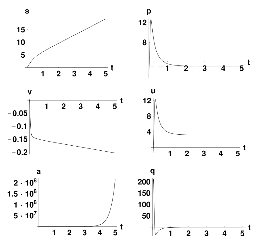
Figure 1: Dependence of functions $u$, $p$, $q$, $s$, $v$ and $a=\exp(s)$ for $\omega=500$, $N=10$, $B=0$ and $u_{0}=-1$, $p_{0}=1$, $q_{0}=-10$.

Figure 2: Dependence of functions $u$, $p$, $q$, $s$, $v$ and $a=\exp(s)$ for $\omega=500$, $N=100$, $B=0$ and $u_{0}=0.1$, $p_{0}=0.1$, $q_{0}=0.1$.

Figure 3: Dependence of functions $u$, $p$, $q$, $s$, $v$ and $a=\exp(s)$ for $\omega=500$, $N=10$, $B=0$ and $u_{0}=3$, $p_{0}=2.8$, $q_{0}=1$.

Figure 4: Dependence of functions $s$ and $v$ for $\omega=500$, $N=10$, $u_{0}=1$, $p_{0}=1$, $q_{0}=1$ and different values of $B$:
left panel: 1 – $B=0$, 2 – $B=10^{3}$, 3 – $B=10^{6}$, 4 – $B=10^{9}$.
right panel: 1 – $B=0$, 2 – $B=-10$, 3 – $B=-40$, 4 – $B=-60$.

Having so different types of numerical solutions it is useful to discuss a possibility to construct any type of analytical solutions. This will be presented in the next section. Also the condition of structural stability is of great importance; it will be considered in detail in the last section.

4 Non-stationary solutions

In the input equations one can exchange the independent variable $t$ and any of the dependent variables. For example, choosing $u$ as new independent variable we can rewrite equations (3) in the following form

$$qt_{u} = 1\,,\qquad qs_{u}=p\,,\qquad qv_{u}=u-p\,,$$

$$qp_{u} = -2p^{2}+\frac{1}{1-\alpha}(q+up+u^{2})\,,$$ (4.1)

$$qq_{u} = -3pq-\frac{u}{1-\alpha}(q+up+u^{2})+2(1+\nu)u^{3}+\beta(p-u)+B\textrm{e}^{-3s}\,.$$

Instead of choosing $u$ as new independent variable we can also choose any other dependent variable, for example $q$. This case is of particular interest because, for $q=0$, there exists the stationary solution (3.6) of the basic equations (3). Therefore when $q\neq 0$ we will get the time-dependent solution according with the first of the following equations

$$Rt_{q} =1\,,\qquad Rs_{q}=p\,,\qquad Rv_{q}=u-p\,,$$ (4.2)

$$Rp_{q} =-2p^{2}+\frac{1}{1-\alpha}(q+up+u^{2})\,,\qquad Ru_{q}=q\,,$$

$${\rm where}\quad R\equiv -3pq-\frac{u}{1-\alpha}(q+up+u^{2})+2(1+\nu)u^{3}+\beta(p-u)+B\textrm{e}^{-3s}\,.$$

In view of the polynomial dependencies of (4.1) and (4.2) upon $u$ and $q$ it is possible to look for solutions in form of an infinite series in these variables.

4.1 Series in $u$

(a) Let us start with the particular case $B=0$. Then we use the following representation for $q$ and $p$

$$q=\sum\limits_{n=0}^{\infty}A_{n}u^{n}\,,\quad p=\sum\limits_{n=0}^{\infty}B_{n}u^{n}\,,$$ (4.3)

while the remaining dependencies are obtained by integrating the first three equations in (4.1) for $t$, $s$ and $v$. Substitution of (4.3) into (4.1) yields an infinite set of equations for the coefficients $A_{n}$ and $B_{n}$:

$$\sum\limits_{j=0}^{k}\Big{(}(k+1-j)A_{k+1-j}A_{j}+3B_{k-j}A_{j}\Big{)}-2(1+\nu)\delta_{k,3}+\beta\delta_{k,1}-\beta B_{k}$$

$$\hphantom{\sum\limits_{j=0}^{k}}+\frac{1}{1-\alpha}\Big{(}\delta_{k,3}+A_{k-1}(1-\delta_{k,0})+B_{k-2}(1-\delta_{k,0})(1-\delta_{k,1})\Big{)}=0\,,$$ (4.4)

$$\sum\limits_{j=0}^{k}\Big{(}(k+1-j)B_{k+1-j}A_{j}+2B_{k-j}B_{j}\Big{)}-\frac{1}{1-\alpha}\Big{(}\delta_{k,2}+A_{k}+B_{k-1}(1-\delta_{k,0})\Big{)}=0\,.$$

Of particular interest are those values of the parameters and initial values when these series are truncated, i.e., reduce to finite sums. In this case the requirement of vanishing for the coefficients $A_{k}$ and $B_{k}$ for $k>k_{\textrm{ max}}$ yields some additional conditions imposed on the coefficients $A_{k}$ and $B_{k}$, that can be fulfilled only for some particular values of the parameters involved. Below we present two examples of such solutions.

(a1)   The first example is valid for $\alpha=0$ and $k_{\rm max}=2$ and is given by the formulas

$$\begin{array}[]{l}A_{0}=B_{0}=A_{1}=B_{2}=0\,,\quad A_{k}=B_{k}=0\,,\quad k\geq 3,\\ B_{1}=1\,,\quad A_{2}=-1\pm\sqrt{1+\nu}<0\,,\\ \mbox{}\\ \displaystyle{s=s_{0}-(1/A_{2})\ln\left(1-A_{2}u_{0}(t-t_{0})\right)\,,\quad v=v_{0}=const.\,,}\\ \mbox{}\\ \displaystyle{q=A_{2}u^{2}\,,\quad u=p=\frac{u_{0}}{1-A_{2}u_{0}(t-t_{0})}\,.}\end{array}$$ (4.5)

This solution confirms that different types of behavior of solutions are possible depending upon the initial conditions. For $u_{0}=p_{0}>0$ we have transition to the stationary state with zero asymptotic values of $u$ and $p$ at $t\to\infty$, while for $u_{0}<0$ we have an explosion–type behavior whose singularity lies at $t-t_{0}=1/(A_{2}u_{0})$. The scalar curvature is positive and, in the limit $t\rightarrow\infty$, approaches $6\,(1\pm\sqrt{1+\nu})(1\mp\sqrt{1+\nu})^{-2}\,t^{-2}$.

The solution described by formulas (4.5) is valid for $\alpha=0$ and corresponds to $p=u$. However, in this case a more general form of the behavior of functions $q$ and $t$ upon $u$ (as compared to (4.5) ) can be obtained that is given as follows ($C=const.$):

$$t-t_{0}=\mp\frac{1}{2C}\int\limits_{r_{0}}^{r}\!\textrm{ d}r\left(\sqrt{1+\nu}-1-r\right)^{-\frac{3}{4}-\frac{1}{4\sqrt{1+\nu}}}\left(\sqrt{1+\nu}+1+r\right)^{-\frac{3}{4}+\frac{1}{4\sqrt{1+\nu}}}\,,$$ (4.6)

$$s=s_{0}+\frac{1}{4\sqrt{1+\nu}}\ln\left(\frac{\sqrt{1+\nu}+1+r}{\sqrt{1+\nu}-1-r}\right)\,,\quad v=v_{0}=const.\,,$$

$$q=u^{2}r\,,\quad u=p=\pm C\left(\sqrt{1+\nu}-1-r\right)^{-\frac{1}{4}+\frac{1}{4\sqrt{1+\nu}}}\left(\sqrt{1+\nu}+1+r\right)^{-\frac{1}{4}-\frac{1}{4\sqrt{1+\nu}}}\,.$$

The result of the previous case (4.5) arises if we impose the restriction $r_{u}=0$ that leads to constant values of $r=-1\pm\sqrt{1+\nu}$.

Obviously, as long as $p=u$ these solutions are quite special since they correspond to a constant dilaton. Furthermore, because of $p=u$ the solution does not depend on $\beta$ (and $G$)!

(a2)   The second example is valid for $\alpha=1$, $k_{\textrm{ max}}=4$, and is given by the formulas

$$A_{0}=B_{0}=A_{1}=B_{2}=A_{3}=B_{4}=0\,,\quad A_{k}=B_{k}=0\,,\quad k\geq 5,$$ (4.7)

$$B_{1}=1\,,\quad A_{2}=-2\,,\quad A_{4}=-B_{3}=2\nu/\beta\,,$$

$$t-t_{0}=\frac{1}{2u}-\frac{1}{2u_{0}}+\frac{1}{2\sqrt{-\beta/\nu}}\left(\arctan\frac{u}{\sqrt{-\beta/\nu}}-\arctan\frac{u_{0}}{\sqrt{-\beta/\nu}}\right)\,,$$

$$s=s_{0}-\frac{1}{4}\ln\left(\frac{u^{2}(u^{2}-\beta/\nu)}{u_{0}^{2}(u_{0}^{2}-\beta/\nu)}\right)\,,\quad v=v_{0}+\frac{1}{2}\ln\left(\frac{u^{2}-\beta/\nu}{u_{0}^{2}-\beta/\nu}\right)\,,$$

$$p=u\left(1-\frac{2\nu}{\beta}\,u^{2}\right)\,,\quad q=-2u^{2}\left(1-\frac{\nu}{\beta}\,u^{2}\right)\,.$$

This solution may be obtained also directly from Eqs. (2.11) and (2.12) where we used the conformal time $\eta$. Indeed, putting $B=0$ in (2.11) and substituting into (2.3) we get

$$\textrm{d}t=\frac{1}{4}\,\frac{\textrm{d}q}{q}\sqrt{({\nu}/{\beta})+(c_{3}^{2}/c_{2}^{2})q},\quad q=\left(c_{1}+c_{2}\eta\right)^{4}\,,$$

which is easily integrated as

$$t=const.+\frac{1}{2}\left(\sqrt{{\nu}/{\beta}+({c_{3}^{2}}/{c_{2}^{2}})q}-\sqrt{-{\nu}/{\beta}}\arctan\sqrt{-1-({c_{3}^{2}}/{c_{2}^{2}})(\beta/\nu)q}\right)\,.$$

Making use of the definition of $u=v_{t}+s_{t}=a_{\eta}/a^{2}+v_{\eta}/a$ we get, after differentiation of (2.11) and (2.12), the following relation between $u$ and $a$:

$$u^{-1}={(c_{1}+c_{2}\eta)a(\eta)}/c_{2}=\sqrt{({\nu}/{\beta})+({c_{3}^{2}}/{c_{2}^{2}})q}\,.$$

Eliminating $q$ with the help of the last formula from the expression for $t$ we get

$$t=const.+\frac{1}{2}\left(\frac{1}{u}-\sqrt{-{\nu}/{\beta}}\arctan\frac{1}{\sqrt{-\nu/\beta}u}\right)\,,$$

which coincides with (4.7) if we take into account $\arctan x=\pi/2-\arctan(1/x)$. The rest of Eqs. (4.7) may be checked immediately.

In the limit $(t-const.)\to 0$ the last formula gives $u\sim(t-const.)^{-1/3}\,$ ; in the opposite limit $t/\sqrt{-\nu/\beta}>>1$ we have $u\sim(1/2)\left(t-const.+(\pi/4)\sqrt{-\nu/\beta}\right)^{-1}$.

Even in the case of $B\neq 0$, when we can hardly find the analytical dependence of $t$ upon $\eta$, the use of the formula (2.3) can help to find the dependence of $t$ upon $\eta$ by quadratures:

$$t=const+\int\frac{\textrm{d}p}{p}\sqrt{({\nu}/{\beta})+(2B/\beta c_{2}^{3})p^{3}+(c_{3}^{2}/c_{2}^{2})p^{4}},\quad p=\left(c_{1}+c_{2}\eta\right)\,,$$

and formulas (2.11), (2.12) have the form

$$a=(c_{2}/p)\sqrt{({\nu}/{\beta})+(2B/\beta c_{2}^{3})p^{3}+(c_{3}^{2}/c_{2}^{2})p^{4}},\quad v=\ln(p/a)\,.$$

The behavior of $a$ and $v$ upon $t$, resulting from Eqs. (4.6) for $B=0$ as well as (2.11), (2.12) for $B\neq 0$ will be obtained by numerical integration. Some characteristic plots, related to these equations and (4.7), are shown in Fig. 5.

Figure 5: Characteristic behavior of $a(t)$ and $v(t)$ resulting for $B=0$ from (a) equations (4.6) for $C=1$ and $v_{0}=1$ (first, top panel), (b) equations (4.7) for $N=100,G=1$ (second panel); and from equations (2.11,2.12) for $N=100,c_{2}=1,\,c_{3}^{2}=0.1$ with (c) $B=10$ (third panel) and (d) $B=-0.45$, (bottom, fourth panel), respectively.

(b) In the general case when $B\neq 0$ we use the following representation for $q$, $p$ and $s$

$$q=\sum\limits_{n=0}^{\infty}A_{n}u^{n}\,,\quad p=\sum\limits_{n=0}^{\infty}B_{n}u^{n}\,,\quad s=s_{0}-\frac{1}{3}\ln\Big{(}\sum\limits_{n=0}^{\infty}C_{n}u^{n}\Big{)}\,,$$ (4.8)

while the remaining dependencies are obtained by integrating the equations in (4.1) for $t$ and $v$. Substitution of (4.8) into (4.1) yields an infinite set of equations for the coefficients:

$$\sum\limits_{j=0}^{k}\Bigl{(}(k+1-j)A_{k+1-j}A_{j}+3B_{k-j}A_{j}\Bigr{)}$$ (4.9)

$$\hphantom{\sum\limits_{j=0}^{k}(k+1-j)}-2(1+\nu)\delta_{k,3}+\beta\delta_{k,1}-\beta B_{k}-Be^{-3s_{0}}C_{k}$$

$$\hphantom{\sum\limits_{j=0}^{k}(k+1-j)}+\frac{1}{1-\alpha}\left(\delta_{k,3}+A_{k-1}(1-\delta_{k,0})+B_{k-2}(1-\delta_{k,0})(1-\delta_{k,1})\right)=0\,,$$

$$\sum\limits_{j=0}^{k}\Bigl{(}(k+1-j)B_{k+1-j}A_{j}+2B_{k-j}B_{j}\Bigr{)}$$

$$\hphantom{\sum\limits_{j=0}^{k}(k+1-j)}-\frac{1}{1-\alpha}\left(\delta_{k,2}+A_{k}+B_{k-1}(1-\delta_{k,0})\right)=0\,,$$

$$\sum\limits_{j=0}^{k}\Bigl{(}(k+1-j)C_{k+1-j}A_{j}+3C_{k-j}B_{j}\Bigr{)}=0\,.$$

Again, we present two examples of solutions that correspond to truncated series (4.8) for some $k>k_{\rm max}$.

(b1)   The first solution corresponds to $\alpha=0$, $k_{\textrm{ max}}=2$

$$A_{0}=B_{0}=C_{0}=A_{1}=C_{1}=B_{2}=C_{2}=0\,,\quad A_{k}=B_{k}=C_{k+1}=0\,,\quad k\geq 3\,,$$ (4.10)

$$B_{1}=1\,,\quad A_{2}=-1\,,\quad C_{3}=1\,,$$

$$s=-(1/3)\ln(-7u_{0}^{3}/9B)+\ln\left(1+u_{0}(t-t_{0})\right)\,,\quad v=v_{0}=const.\,,$$

$$u=p=\frac{u_{0}}{1+u_{0}(t-t_{0})}\,,\quad q=-\left(\frac{u_{0}}{1+u_{0}(t-t_{0})}\right)^{2}\,.$$

Here again we see the effect of explosive behavior for $u_{0}<0$ at $t-t_{0}\to-(1/u_{0})$ and asymptotic stability at $t\to\infty$ in the opposite limit $u_{0}>0$ similar to the observation above. Again, the curvature is positive and approaches $6/t^{2}$.

(b2)   The second solution corresponds to some $\alpha\neq 0$, $k_{\rm max}=2$:

$$A_{0}=B_{0}=C_{0}=A_{1}=B_{2}=C_{2}=0\,,\quad A_{k}=B_{k}=C_{k}=0\,,\quad k\geq 3,$$ (4.11)

$$B_{1}=\pm(1/2)\sqrt{1+\nu}\,,\quad A_{2}=-3B_{1}=\mp(3/2)\sqrt{1+\nu}\,,$$

$$C_{1}=\frac{\beta}{B}(1-B_{1})\exp\left(3s_{0}\right)\,,\quad\alpha=\left(\frac{1-B_{1}}{B_{1}}\right)^{2}\equiv 1+4\frac{1\mp\sqrt{1+\nu}}{1+\nu}\,,$$

$$s=-(1/3)\ln(\beta(1-B_{1})u_{0}/B)+\frac{1}{3}\ln\left(1+3B_{1}u_{0}(t-t_{0})\right)\,,$$

$$v=v_{0}+\frac{1-B_{1}}{3B_{1}}\ln\left(1+3B_{1}u_{0}(t-t_{0})\right)\,,\quad u=\frac{u_{0}}{1+3B_{1}u_{0}(t-t_{0})}\,,$$

$$q=-3B_{1}\left(\frac{u_{0}}{1+3B_{1}u_{0}(t-t_{0})}\right)^{2}\,,\quad p=B_{1}\frac{u_{0}}{1+3B_{1}u_{0}(t-t_{0})}\,.$$

Here, the system demonstrates explosive behavior for $B_{1}u_{0}<0$, while for $B_{1}u_{0}>0$ we have vanishing $u$, $q$ and $p$ for $t\to\infty$, and the raise of $s$ and $v$ is softer than in the stationary case. Here, the curvature is negative and approaches $-(2/3)\,t^{-2}$.

4.2 Series in $q$

Here we will examine only the particular case of $B=0$. Then we use the following representation for $u$ and $p$

$$u=\sum\limits_{n=0}^{\infty}A_{n}q^{n}\,,\quad p=\sum\limits_{n=0}^{\infty}B_{n}q^{n}\,,\quad$$ (4.12)

while the remaining dependencies are obtained by integrating the first three equations in (4.2) for $t$, $s$ and $v$. Substitution of the expansions (4.12) into the next two equations in (4.2) yields the following infinite set of equations for the coefficients:

$$\sum\limits_{j=0}^{k}(k+1-j)A_{k+1-j}R_{j}-\delta_{k,1}=0\,,$$ (4.13)

$$\sum\limits_{j=0}^{k}\Bigl{(}(k+1-j)B_{k+1-j}R_{j}+2B_{k-j}B_{j}\Bigr{)}$$

$$\hphantom{\sum\limits_{j=0}^{k}\Bigl{(}(k+1-j)B_{k+1-j}R_{j}}-\frac{1}{1-\alpha}\Big{(}\delta_{k,1}+\sum\limits_{j=0}^{k}A_{j}\left(A_{k-j}+B_{k-j}\right)\Bigr{)}=0\,,$$

$${\textrm{ where}}\quad{R_{j}} =(\delta_{j,0}-1)\left(3B_{j-1}+\frac{1}{1-\alpha}A_{j-1}\right)+\beta(B_{j}-A_{j})$$ (4.14)

$$+\sum\limits_{i=0}^{j}\sum\limits_{l=0}^{i}A_{l}A_{i-l}\left(2(1+\nu)A_{j-1}-\frac{1}{1-\alpha}\left(B_{j-1}+A_{j-1}\right)\right)\,.$$

Despite being of principal interest this set of equations is quite complicated. There exists one evident truncation of the series (4.12) namely when only zero order terms are taken into account, $A_{0}\neq 0$, $B_{0}\neq 0$, whilst $A_{k}=B_{k}=0$ for $k\geq 1$. This truncation corresponds to $q=0$ and the stationary solution (3.8). Unfortunately, in the case $q\neq 0$ we were not able to find a nontrivial truncation of these series.

5 Stability analysis

5.1 Small perturbations

Here, we consider only the case $B=0$. Then the basic equations have stable solutions of the form (3.6). By linearizing these equations with respect to small perturbations $\delta u=u-u_{\textrm{ st}}$, $\delta q=q$, $\delta p=p-p_{\textrm{ st}}$ we obtain a system of linear equations that admit solutions of the form $\delta u\propto U\,\textrm{ e}^{\lambda t}$, $\delta q\propto Q\,\textrm{ e}^{\lambda t}$ and $\delta p\propto P\,\textrm{ e}^{\lambda t}$ where $\lambda$ obeys the characteristic equation

$$\left[\lambda^{2}+\lambda\left(3p_{\textrm{ st}}+\frac{u_{\textrm{ st}}}{1-\alpha}\right)+\frac{u_{\textrm{ st}}}{1-\alpha}(2p_{\textrm{ st}}+3u_{\textrm{ st}})+\beta-6(1+\nu)u_{\textrm{ st}}^{2}\right]$$

$$\times\left(\lambda+4p_{\textrm{ st}}-\frac{u_{\textrm{ st}}}{1-\alpha}\right)-\frac{1}{1-\alpha}\left(\beta-\frac{u_{\textrm{ st}}^{2}}{1-\alpha}\right)(\lambda+p_{\textrm{ st}}+2u_{\textrm{ st}})=0\,.$$ (5.1)

Below, on Fig. 6, we present a plot illustrating the dependence of real parts of solutions of the equation (5.1) upon the parameter $\omega$. The graphic shows that there exist stable solutions in a large region of the parameter $\omega$.

Figure 6: Dependence of real parts of solutions of the characteristic equation (5.1) upon $\omega$ that demonstrates the existence of stable (curves $1,\ 2$ and $3$ on the left panel correspond to negative real parts) and unstable (the curve $3$ on the right panel corresponds to the positive real part) stationary solutions.

The corresponding numerical solutions of input equations (3) on Fig. 7 shows the behavior of the functions $s$ and $v$ in the vicinity of the stationary state.

Figure 7: Dependence of functions $s$ and $v$ for $\omega=500$, $N=10$ for stable (left panel) and unstable (right panel) solutions.

Straight lines (curves 1) correspond to stationary solutions (3.6) with $u_{\textrm{ st}}=3,19549$, $p_{\textrm{ st}}=3,20687$ for the left panel and $u_{\textrm{st}}=-138,843$, $p_{\textrm{ st}}=69,5447$ for the right panel. For the left panel curves 2 relate to $u_{0}-u_{\textrm{ st}}=-0.02$, $p_{0}-p_{\textrm{ st}}=0.01$ and $q_{0}=0.01$; curves 3 relate to $u_{0}-u_{\rm st}=-0.02$, $p_{0}-p_{\textrm{ st}}=-0.01$ and $q_{0}=-0.01$. For the right panel curves 2 relate to $u_{0}-u_{\textrm{ st}}=-0.02$, $p_{0}-p_{\textrm{st}}=-0.01$ and $q_{0}=0.01$; curves 3 relate to $u_{0}-u_{\textrm{st}}=0.01$, $p_{0}-p_{\textrm{ st}}=-0.01$ and $q_{0}=-0.01$.

5.2 Transition to the stationary solution

It is evident that for initial values that are close enough to the stable stationary values we can get an analytical solution for arbitrary initial values $u(t=0)=u_{0}$, $p(t=0)=p_{0}$ and $q(t=0)=q_{0}$. This solution is given by linear combinations of exponential functions defined by solutions of the characteristic equations presented in the previous subsection with coefficients, depending upon the initial values

$$q=D_{1}\exp({\lambda_{1}t})+D_{2}\exp({\lambda_{2}t})+D_{3}\exp({\lambda_{3}t})\,,$$ (5.2)

$$u=u_{\textrm{st}}+(D_{1}/\lambda_{1})\exp({\lambda_{1}t})+(D_{2}/\lambda_{2})\exp({\lambda_{2}t})+(D_{3}/\lambda_{3})\exp({\lambda_{3}t})\,,$$

$$p=p_{\textrm{st}}+D_{1}\Lambda_{1}\exp({\lambda_{1}t})+D_{2}\Lambda_{2}\exp({\lambda_{2}t})+D_{3}\Lambda_{3}\exp({\lambda_{3}t})\,,$$

$${\rm with}\qquad\Lambda_{i}=\frac{(p_{\textrm{st}}+2u_{\textrm{st}}+\lambda_{i})/\lambda_{i}}{(4p_{\textrm{st}}+\lambda_{i})(1-\alpha)-u_{\textrm{st}}}\,.$$

Here the constants $D_{1}$, $D_{2}$ and $D_{3}$ are expressed in terms of the initial values as follows:

$$D_{1}=\frac{\Delta_{1}}{\Delta_{0}}\,,\quad D_{2}=\frac{\Delta_{2}}{\Delta_{0}}\,,\quad D_{3}=\frac{\Delta_{3}}{\Delta_{0}}\,,$$ (5.3)

$$\Delta_{0}=\Lambda_{1}\left(\frac{1}{\lambda_{3}}-\frac{1}{\lambda_{2}}\right)+\Lambda_{2}\left(\frac{1}{\lambda_{1}}-\frac{1}{\lambda_{3}}\right)+\Lambda_{3}\left(\frac{1}{\lambda_{2}}-\frac{1}{\lambda_{1}}\right)\,,$$

$$\Delta_{1}=(u_{0}-u_{\textrm{st}})\left({\Lambda_{2}}-{\Lambda_{3}}\right)+q_{0}\left(\frac{\Lambda_{3}}{\lambda_{2}}-\frac{\Lambda_{2}}{\lambda_{3}}\right)+(p_{0}-p_{\textrm{st}})\left(\frac{1}{\lambda_{3}}-\frac{1}{\lambda_{2}}\right)\,,$$

$$\Delta_{2}=(u_{0}-u_{\textrm{st}})\left({\Lambda_{3}}-{\Lambda_{1}}\right)+q_{0}\left(\frac{\Lambda_{1}}{\lambda_{3}}-\frac{\Lambda_{3}}{\lambda_{1}}\right)+(p_{0}-p_{\textrm{st}})\left(\frac{1}{\lambda_{1}}-\frac{1}{\lambda_{3}}\right)\,,$$

$$\Delta_{3}=(u_{0}-u_{\textrm{st}})\left({\Lambda_{1}}-{\Lambda_{2}}\right)+q_{0}\left(\frac{\Lambda_{2}}{\lambda_{1}}-\frac{\Lambda_{1}}{\lambda_{2}}\right)+(p_{0}-p_{\textrm{st}})\left(\frac{1}{\lambda_{2}}-\frac{1}{\lambda_{1}}\right)\,.$$

Integrating the remaining equations we get the following formulas for $s$ and $v$ that describe the transition to the stationary state

$$s=s_{0} +(t-t_{0})p_{\textrm{st}}+D_{1}\ \frac{\Lambda_{1}}{\lambda_{1}}\left(\textrm{e}^{\lambda_{1}t}-\textrm{e}^{\lambda_{1}t_{0}}\right)$$ (5.4)

$$+D_{2}\ \frac{\Lambda_{2}}{\lambda_{2}}\left(\textrm{e}^{\lambda_{2}t}-\textrm{e}^{\lambda_{2}t_{0}}\right)+D_{3}\ \frac{\Lambda_{3}}{\lambda_{3}}\left(\textrm{e}^{\lambda_{3}t}-\textrm{e}^{\lambda_{3}t_{0}}\right)\,,$$

$$v=v_{0} +(t-t_{0})(u_{\textrm{st}}-p_{\textrm{st}})+\frac{D_{1}}{\lambda_{1}}\left(\frac{1}{\lambda_{1}}-{\Lambda_{1}}\right)\left(\textrm{e}^{\lambda_{1}t}-\textrm{e}^{\lambda_{1}t_{0}}\right)$$

$$+\frac{D_{2}}{\lambda_{2}}\left(\frac{1}{\lambda_{2}}-{\Lambda_{2}}\right)\left(\textrm{e}^{\lambda_{2}t}-\textrm{e}^{\lambda_{2}t_{0}}\right)+\frac{D_{3}}{\lambda_{3}}\left(\frac{1}{\lambda_{3}}-{\Lambda_{3}}\right)\left(\textrm{e}^{\lambda_{3}t}-\textrm{e}^{\lambda_{3}t_{0}}\right)\,.$$

It is clearly seen that the asymptotic behaviour of the functions $s$ and $v$ depends linear upon $t$, and the slope of these lines is defined by the stationary values, while the slope at the point $t=0$ is defined by the initial values.

In order to compare the perturbative solutions (5.4) with the exact ones of the basic equations (3) we considered the behaviour of $s$, $v$, $u$, $p$, $q$ and $a$ for initial values $u_{0}$, $p_{0}$ and $q_{0}$ that are close to the stationary values $u_{\textrm{st}}$, $p_{\textrm{st}}$ and $q=0$ for $\omega=500,B=0$ and different values of $N$. An example, for $N=10$, is presented in Fig. 8.

Figure 8: Exact numerical (solid line) and approximate analytical (5.4) (dashed lines) solutions of basic equations (3) for $\omega=500$, $N=10$, $B=0$, $q_{0}=1$ and initial values $u_{0}=p_{0}=2$ close to stationary ones $u_{\textrm{st}}=3.19549$, $p_{\textrm{st}}=3.20687$.

These plots demonstrate that there is only a small discrepancy between exact and approximate solutions for physically interesting quantities $a$ (resp. $s$) and $v$, whereas the difference for $u,p$ and $q$ is somewhat larger. These differences decrease for increasing values of $N$. Obviously, the exact solution is approximated very fast.

But, even if the initial values differ substantially from the stationary ones the approximate formulas still give a satisfactory accuracy for $u_{0}=p_{0}$. Moreover, as the input equations are linear in $q$ it appears that the approximate solution is sometimes valid even when the initial value of $q_{0}$ is not small. This is clearly seen in Fig. 9.

Figure 9: Exact numerical (solid line) and approximate analytical (5.4) (dashed lines) solutions of basic equations (3) for $\omega=500$, $N=10$, $B=0$, $q_{0}=50$ and initial values $u_{0}=p_{0}=0.5$ not close to stationary ones $u_{\textrm{st}}=3.19549$, $p_{\textrm{st}}=3.20687$.

Also in these cases the stationary solution is approximated after a few units of time.

6 Conclusion

Analysing the evolution equations in conformal time we were able to present a new exact solution (for $\alpha=1\sim\omega=7/6$). After transforming to physical time we found ‘stationary’ solutions of the corresponding basic set of first order differential equations (restricted to $B=0$) which generalize the inflationary solution already known from an earlier study [1]. The numerical analysis of the basic set showed quite different types of dilaton-driven evolution in cases $B=0$ as well as $B\neq 0$: In a wide range of the parameters of the theory the stationary solution is approximated very fast; furthermore, there are also quite different non-stationary solutions showing explosion type, oscillatory as well as collapsing behaviour. Seeking solutions as (finite) power series we were able to find additional particular solutions of the basic set with a (modified) logarithmic raise of $s(t)$ which, in comparison with the stationary solution raising linearly, lead to a more soft inflation; however, nontrivial dilatonic behaviour results only in the cases (a2) and (b2). Finally, we presented a stability analysis for the case $B=0$ thereby showing how the transition to the stationary solution occurs.

It is very interesting that the mathematical methods applied here to study the conformally flat Universe with time-dependent dilaton solutions leading to effective forth order equations of motion are general enough to be used also in various related contexts. As an immediate application we may consider the problem of quantum creation and annihilation of Anti de Sitter Universe and Anti de Sitter black holes due to quantum effects of (dilaton coupled) matter. Such a phenomenon has been investigated recently in Ref. [9]. In these works the anomaly induced effective action for dilaton coupled spinors has been used similarly to the present paper. Moreover, the Anti de Sitter Universe in conformally flat coordinates looks very similar to the de Sitter (inflationary) Universe: the corresponding equations of motion are - with some change of signs - almost the same as Eqs. (2.6) and (2.7) (where, however, the role of time is played by the radial coordinate in AdS Universe). Hence, our results may be used in the construction of other variants of the asymptotically AdS solutions which have been found in Ref. [9].

Acknowledgement
The authors are very much indebted to S.D. Odintsov for numerous stimulating discussions and a careful reading of the manuscript. V.F. Kovalev acknowledges for a grant of Saxonian Ministry of Sciences and Arts.

References

References

- [1] B. Geyer, S.D. Odintsov and S. Zerbini, Phys. Lett B 460 (1999) 58.
- [2] V. Faraoni, E. Gunzig and P. Nardone, Conformal transformations in classical gravitational theories and in cosmology, Fundamentals of Cosmic Physics 20 (1999) 121.
- [3] C.M. Will, Theory and Experiments in Gravitational Physics, Cambridge, 1993.
- [4] J. Polchinski, String Theory, Cambridge, 1998.
-
[5]
D. La and P.J. Steinhardt, Phys. Rev. Lett.
62 (1989) 376;
E.W. Kolb, D. Salopek and M.S. Turner, Phys. Rev D42 (1990) 3925;
for a review, see:
E. Kolb and M. Turner, The Very Early Universe, New York, 1994. -
[6]
J.D. Barrow, Phys. Rev. D59 (1999) ;
J.D. Barrow and J. Magueijo, Class. Quant. Grav. 16 (1999) 1435. -
[7]
S. Nojiri and S.D. Odintsov,
Phys. Rev. D57 (1998) 2363;
Phys. Lett. B426 (1998) 29;
B444 (1998) 92;
S. Ichinose and S.D. Odintsov, Nucl. Phys. B539 (1999) 634;
P. van Nieuwenhuizen, S. Nojiri and S.D. Odintsov, Phys. Rev. D60 084014. - [8] Nail H. Ibragimov, Elementary group analysis and ordinary differential equations, John Wiley & Sons, Chichester-Weinheim, 1999.
-
[9]
I. Brevik and S.D. Odintsov, hep-th/9912032, Phys. Lett. (to appear)
S. Nojiri, S.D. Odintsov, and S. Zerbini, hep-th/0001192.