BUTP–00/32

hep-ph/0011093

The decay $\bi{b\to sg}$ at NLL in the Standard Model
P. Liniger

Institut für theoretische Physik, Universität Bern,

Sidlerstrasse 5, 3012 Bern, Switzerland

ABSTRACT

I present the Standard Model calculation of the decay rate $\Gamma(b\to sg)$ ($g$ denotes a gluon) at next-to-leading logarithms (NLL). In order to get a meaningful physical result, the decay $b\to sgg$ and certain contributions of $b\to s\bar{f}f$ (where $f$ are the light quark flavours $u$, $d$ and $s$) have to be included as well. Numerically we get ${\mathcal{B}}^{\rm NLL}(b\to sg)=(5.0\pm 1.0)\cdot 10^{-3}$ which is more than a factor 2 larger than the leading logarithmic result ${\mathcal{B}}^{\rm LL}(b\to sg)=(2.2\pm 0.8)\cdot 10^{-3}$. Further, I consider the impact of this contribution on the charmless hadronic branching ratio ${\mathcal{B}}_{c\!\!/}$, which could be used to extract the CKM-ratio $|V_{ub}/V_{cb}|$ with more accuracy. Finally, I have a short look at ${\mathcal{B}}_{c\!\!/}$ in scenarios where the Wilson coefficient $C_{8}$ is enhanced by new physics.

Talk presented at the
“UK Phenomenology Workshop on Heavy Flavour and CP Violation”

St John’s College, Durham, 17 - 22 September 2000

Abstract

I present the Standard Model calculation of the decay rate $\Gamma(b\to sg)$ ($g$ denotes a gluon) at next-to-leading logarithms (NLL). In order to get a meaningful physical result, the decay $b\to sgg$ and certain contributions of $b\to s\bar{f}f$ (where $f$ are the light quark flavours $u$, $d$ and $s$) have to be included as well. Numerically we get ${\mathcal{B}}^{\rm NLL}(b\to sg)=(5.0\pm 1.0)\cdot 10^{-3}$ which is more than a factor 2 larger than the leading logarithmic result ${\mathcal{B}}^{\rm LL}(b\to sg)=(2.2\pm 0.8)\cdot 10^{-3}$. Further, I consider the impact of this contribution on the charmless hadronic branching ratio ${\mathcal{B}}_{c\!\!/}$, which could be used to extract the CKM-ratio $|V_{ub}/V_{cb}|$ with more accuracy. Finally, I have a short look at ${\mathcal{B}}_{c\!\!/}$ in scenarios where the Wilson coefficient $C_{8}$ is enhanced by new physics.

1 Introduction

Theoretical studies for inclusive $B$-decays have become accessible due to heavy quark effective theory (HQET). HQET [2, 3] states that the amplitudes of decaying $B$-mesons can be expanded in powers of $(\Lambda_{\rm QCD}/m_{b})$ where the leading term is nothing but the decay of the underlying $b$-quark. Corrections to this start at $\Or(\Lambda_{\rm QCD}^{2}/m_{b}^{2})$ only, which numerically amounts to $\sim 5\%$.

One interesting subclass of inclusive $B$-decays are the charmless ones $B\to X_{c\!\!/}$. They have been thoroughly investigated in the literature: the calculation for $b\to\bar{q}^{\prime}q^{\prime}q$ with $q=d,s$ and $q^{\prime}=u,d,s$ have been available to NLL for quite some time [4, 5, 6, 7] and the missing piece, $b\to sg$, is what is presented here. Due to the sensitivity of the charmless branching ratio ${\mathcal{B}}_{c\!\!/}$ to the poorly known CKM ratio $|V_{ub}/V_{cb}|$, these decays might be used in order to get a better determination of this standard model parameter.

The decay $b\to sg$ turned out to be an interesting issue in the discussion of the ’missing charm puzzle’; for a long time there was a discrepancy between theory and experiment for the average charm multiplicity $n_{c}$ per $B$-decay and for the inclusive semileptonic branching ratio ${\mathcal{B}}_{\rm sl}$ [8]. This issue seems to have settled a bit.

2 Theoretical Framework

The calculation is based on an effective Hamiltonian $\mathcal{H}_{\rm eff}$ obtained by integrating out the heavy degrees of freedom of the standard model (i.e. the $t$-quark and the $W$-boson). Retaining operators up to dimension six, the 5-flavour effective Hamiltonian responsible for $b\to sg$ reads

$$\mathcal{H}_{\rm eff}=-\frac{4G_{F}}{\sqrt{2}}\,V_{ts}^{*}V_{tb}\sum_{i=1}^{8}C_{i}(\mu)O_{i}(\mu),$$ (1)

where $V_{ij}$ are CKM-matrix entries, $C_{i}(\mu)$ the Wilson coefficients and $O_{i}(\mu)$ the relevant operators. As the Wilson coefficients $C_{3-6}$ are small, we only consider the operators

$$O_{1}\,=(\bar{s}_{L}\gamma_{\mu}T^{A}c_{L})\,(\bar{c}_{L}\gamma^{\mu}T^{A}b_{L})\,, O_{2}\,=(\bar{s}_{L}\gamma_{\mu}c_{L})\,(\bar{c}_{L}\gamma^{\mu}b_{L})\,,$$

$$O_{8}\,=\frac{g_{s}}{16\pi^{2}}\,{\bar{m}}_{b}(\mu)\,(\bar{s}_{L}\sigma^{\mu\nu}T^{A}b_{R})\,G^{A}_{\mu\nu}\ .$$ (2)

Here $T^{A}$ stand for the $SU(3)_{\rm{colour}}$ generators. The small CKM matrix element $V_{ub}$ as well as the $s$-quark mass are neglected. The whole work is done in the NDR scheme, i. e. with anticommuting $\gamma_{5}$ and using $\overline{\rm MS}$ subtraction.

3 Contributions

3.1 Virtual Corrections to $O_{1}$ and $O_{2}$

In figure 1 there is the complete set of Feynman diagrams that contribute to $b\to sg$. As these start at $\Or(g_{s}\alpha_{s})$ only (no one loop contributions), the Wilson coefficients $C_{1}$ and $C_{2}$ are needed to leading logarithmic precision only.

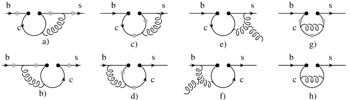
Figure 1: Complete list of two-loop Feynman diagrams for $b\to sg$ associated with the operators $O_{1}$ and $O_{2}$. The crosses denote the possible locations where the gluon is emitted.

The heart of the procedure is to make a Mellin-Barnes representation [9] of the two-loop integrals. That is, after the Feynman parametrization and after integrating over the loop momenta, the remaining expression is of the form $(k^{2}-M^{2})^{-\lambda}$ which can be written as

$$\frac{1}{(k^{2}-M^{2})^{\lambda}}=\frac{1}{(k^{2})^{\lambda}}\,\frac{1}{\Gamma(\lambda)}\,\frac{1}{2\pi\rmi}\,\int_{\gamma}\rmd{s}(-M^{2}/k^{2})^{s}\Gamma(-s)\Gamma(\lambda+s)\;,$$ (3)

where, in the actual calculation, $M^{2}$ (resp. $k^{2}$) is $m_{c}^{2}$ (resp. $m_{b}^{2}$) times some combination of the Feynman parameters and $\gamma$ is a path in the $s$-plane parallel to the imaginary axis with $-\lambda<\Re(s)<0$. This representation leads naturally to an expansion in $z=m_{c}^{2}/m_{b}^{2}$ which is numerically around $0.1$. All contributions up to $z^{3}$ are retained. In the end, the result consists of powers and logarithms of $z$ only.

The matrix elements for the operators $O_{1/2}$ contain UV-divergences which are removed by renormalization; there are no IR problems and also singularities due to $m_{s}=0$ are absent.

3.2 Virtual Corrections to $O_{8}$

Some comments on the contributions of $O_{8}$ are in order. The relevant diagrams are displayed in figure 2.

Figure 2: Complete list of Feynman diagrams associated with the operator $O_{8}$. The analogues of a), c) and d), where the virtual gluon hits the $b$-quark instead of the $s$-quark, are not shown explicitly. The real gluon can be attached to any of the crosses shown in a).

Some technical details of the calculation: for this part, the $s$-quark mass has not been set to zero but was kept as a regulator in order to distinguish between mass-singularities and IR-singularities.

As $O_{8}$ contributes to $b\to sg$ at tree-level already, the Wilson coefficient $C_{8}$ is needed at NLL precision [10]. Also due to the appearance of the gluon field strength in the operator, $Z_{3}$ enters upon renormalization. From the gluon self-energy there are logarithms $\ln(\mu/m_{f})$ (with $f=u,d,s$) entering the calculation. In order to avoid the singularities that would show up when the respective masses are set to zero, also the decay $b\to s\bar{f}f$ (arising from $O_{8}$ only) was included.

After renormalization $\Gamma_{8}(b\to sg+s\bar{f}f)$ has the form

$$\Gamma_{8}(b\to sg+s\bar{f}f)=\sum_{\begin{array}[]{l}\scriptstyle n,m=0,1,2\\[-3.01389pt] \scriptstyle n+m\leq 2\end{array}}a_{nm}\frac{\ln^{n}(m_{s}/m_{b})}{\epsilon_{\rm IR}^{m}}$$ (6)

where it is anticipated that the remaining singularities will cancel against the gluon bremsstrahlung.

3.3 Bremsstrahlung $b\to sgg$

In order to get a physically meaningful (in particular an IR finite) result, the bremsstrahlung contributions form $O_{1/2/8}$ have to be added. Again (for $O_{8}$ only, as the ones from $O_{1/2}$ are finite anyway) $m_{s}$ is kept as a regulator and the phase space integrals are done in $d=4-2\epsilon$ dimensions. Only the singularities are worked out analytically, the phase space for the finite parts is done numerically.

4 Result

Adding the various pieces, the singularities cancel in fact (according to the KLN-theorem). The result can be cast into a form involving an effective matrix element $\bar{D}$ (where $\Gamma^{\rm NLL}(b\to sg)$ denotes $\Gamma(b\to sg(g))+\Gamma_{8}(b\to s\bar{f}f)$):

$$\Gamma^{\rm NLL}(b\to sg)=\frac{\alpha_{s}m_{b}^{5}}{24\pi^{4}}G_{F}^{2}|V_{ts}^{*}V_{tb}|^{2}|\bar{D}|^{2}+\Gamma^{\rm brems}_{\rm fin}$$ (7)

with

$$\bar{D}= C_{8}^{0,\rm{eff}}+\frac{\alpha_{s}}{4\pi}\,\Bigl{\{}C_{8}^{1,\rm{eff}}-{\textstyle\frac{16}{3}}C_{8}^{0,\rm{eff}}+C_{1}^{0}[\ell_{1}\,\ln(m_{b}/\mu)+r_{1}]$$ (8)

$$+C_{2}^{0}[\ell_{2}\,\ln(m_{b}/\mu)+r_{2}]+C_{8}^{0,\rm{eff}}[(\ell_{8}+8+\beta_{0})\,\ln(m_{b}/\mu)+r_{8}]\Bigr{\}}$$

where $\Gamma^{\rm brems}_{\rm fin}$ denotes the finite bremsstrahlung part which affects the result by $\sim 5\%$ only; $\ell_{1/2}$ and $(\ell_{8}+8+\beta_{0})$ are nothing but the entries of the anomalous dimension matrix $\gamma^{0,\rm eff}_{18/28/88}$ and $r_{1/2/8}$ encode the loop functions. For the Wilson coefficients we have used the perturbative decomposition $C_{i}=C_{i}^{0}+\frac{\alpha_{s}}{4\pi}C_{i}^{1}$.

The branching ratio is given by the expression ${\mathcal{B}}(b\to sg)=\frac{\Gamma^{\rm NLL}(b\to sg)}{\Gamma_{\rm sl}}{\mathcal{B}}_{\rm sl}^{\rm exp}.$

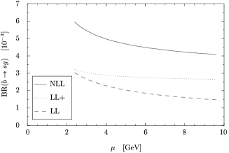
Figure 3: Scale dependence of the function $\bar{D}$ (equation (8)) and the branching ratio in various approximations: the dashed line corresponds to leading order (for $\bar{D}$ this is simply $C_{8}^{0,\rm eff}(\mu)$), the solid line is the full NLL result. For the dotted line we set $r_{1}=r_{2}=r_{8}=0$ (and, for the branching ratio, $\Gamma_{\rm brems}^{\rm fin}=0$ in addition). The dot-dashed line is obtained by putting $r_{2}=0$ only.

The NLL branching ratio still suffers from a big $\mu$-dependence. As is illustrated in figure 3 this is due to $r_{2}$ which is also responsible for the sizable enhancement of the branching ratio. This large factor is multiplied by $\alpha_{s}(\mu)C_{2}(\mu)$ and numerically spoils the cancellation of the $\mu$ dependence which is established through $\ell_{1/2/8}$.

Numerically we get (and reproduce the LL result [11])

$${\mathcal{B}}^{\rm NLL}(b\to sg)=(5.0\pm 1.0)\cdot 10^{-3},\qquad {\mathcal{B}}^{\rm LL}(b\to sg)=(2.2\pm 0.8)\cdot 10^{-3}.$$ (9)

Combining our NLL result with the work of Lenz et al. [5, 6], we calculate the CP-averaged charmless hadronic branching ratio ${\overline{{\mathcal{B}}}}_{c\!\!/}$ and the CP-averaged total charmless branching ratio $\overline{{\mathcal{B}}}(B\to{\rm no\ charm})$ (the errors are estimated by varying the scale $\mu$ in the range $[m_{b}/2,2m_{b}]$)

$${\overline{{\mathcal{B}}}}_{c\!\!/}=(1.88^{+0.60}_{-0.38})\%,\qquad \overline{{\mathcal{B}}}(B\to{\rm no\ charm})=(2.22^{+0.60}_{-0.38})\%.$$ (10)

The latter is very sensitive to $|V_{ub}/V_{cb}|$: varying this ratio in the range $0.06-0.13$ the total charmless branching ratio covers the range $(1.50-2.42)\%$.

5 Remarks on $\bi{n_{c}}$ and $\bi{{\cal B}_{\rm\bf sl}}$

As discussed in the introduction, the theoretical predictions for both, the charm multiplicity $n_{c}$ and the semileptonic branching ratio ${\mathcal{B}}_{\rm sl}$ used to be in disagreement with the experimental data [7]. This discrepancy decreased a lot after the inclusion of the complete NLL corrections to $b\to c\bar{u}q$ and $b\to c\bar{c}q$ ($q=d,s$) [12]. If one allows the renormalization scale $\mu$ to be as low as $m_{b}/4$, then there is a marginal overlap between theory and CLEO- and LEP data [13]. It is therefore a matter of taste if one considers this problem to be solved or if one is inclined towards an enhancement of the Wilson coefficient through non standard model physics. The impact of such an enhancement is displayed in figure 4.

Figure 4: Charmless hadronic branching ratio ${\overline{{\mathcal{B}}}}_{c\!\!/}$ as a function of the ratio $f=C_{8}^{\rm{eff}}(m_{W})/C_{8}^{\rm{eff,SM}}(m_{W})$. The dotted (solid) curve includes the LL (NLL) approximation for $b\to sg$.

References

References

- [1] C. Greub and P. Liniger, hep-ph/0009144; hep-ph/0008071.
-
[2]
I. Bigi et al., Phys. Rev. Lett. 71, 496 (1993);
A. Manohar and M.B. Wise, Phys. Rev. D49, 1310 (1994);
B. Blok et al., Phys. Rev. D49, 3356 (1994);
T. Mannel, Nucl. Phys. B413, 396 (1994);
A. Falk, M. Luke, and M. Savage, Phys. Rev. D49, 3367 (1994). - [3] I. Bigi et al., Phys. Lett. B293, 430 (1992); 297 (1993) 477 (E).
- [4] G. Altarelli and S. Petrarca, Phys. Lett. B261, 303 (1991).
- [5] A. Lenz, U. Nierste and G. Ostermaier, Phys. Rev. D56, 7228 (1997).
- [6] A. Lenz, U. Nierste and G. Ostermaier, Phys. Rev. D59, 034008 (1999).
- [7] A. Lenz, these proceedings.
-
[8]
I. Bigi et al., Phys. Lett. B323, 408 (1994);
A. Falk, M.B. Wise, and I. Dunietz, Phys. Rev. D51, 1183 (1995);
I. Dunietz et al., Eur. Phys. J. C1, 211 (1998);
H. Yamamoto, hep-ph/9912308. -
[9]
V.A. Smirnov, Renormalization and Asymptotic Expansions,
Birkhäuser Basel 1991;
E.E. Boos and A.I. Davydychev, Theor. Math. Phys. 89 1052 (1992);
N.I. Usyukina, Theor. Math. Phys. 79 (1989) 385, 22 211 (1975);
A. Erdelyi (ed.), Higher Transcendental Functions, McGraw New York 1953. - [10] K. Chetyrkin, M. Misiak, and M. Münz, Phys. Lett. B400, 206 (1997); Nucl. Phys. B518, 473 (1998); Nucl. Phys. B520, 279 (1998).
- [11] M. Ciuchini et al. Phys. Lett. B334, 137 (1994);
- [12] E. Bagan et al., Nucl. Phys. B432, 3 (1994); Phys. Lett. B 342, 362 (1995) [E:374, 363 (1996)]; E. Bagan et al., Phys. Lett. B 351, 546 (1995)
- [13] A. Golutvin, plenary talk given at the XXXth International Conference on High Energy Physics, Osaka, Japan, July 2000.