LBNL-46970

UCB-PTH-00/37

LPT-Orsay-00/87

hep-ph/0011081

One loop soft supersymmetry breaking terms in superstring effective theories

Pierre Binétruy,

LPT, Université Paris-Sud, Bat.210 F-91405 Orsay Cedex

Mary K. Gaillard and Brent D. Nelson

Department of Physics, University of California, and

Theoretical Physics Group, 50A-5101, Lawrence Berkeley National Laboratory,

Berkeley, CA 94720, USA

We perform a systematic analysis of soft supersymmetry breaking terms at the one loop level in a large class of string effective field theories. This includes the so-called anomaly mediated contributions. We illustrate our results for several classes of orbifold models. In particular, we discuss a class of models where soft supersymmetry breaking terms are determined by quasi model independent anomaly mediated contributions, with possibly non-vanishing scalar masses at the one loop level. We show that the latter contribution depends on the detailed prescription of the regularization process which is assumed to represent the Planck scale physics of the underlying fundamental theory. The usual anomaly mediation case with vanishing scalar masses at one loop is not found to be generic. However gaugino masses and A-terms always vanish at tree level if supersymmetry breaking is moduli dominated with the moduli stabilized at self-dual points, whereas the vanishing of the B-term depends on the origin of the $\mu$-term in the underlying theory. We also discuss the supersymmetric spectrum of O-I and O-II models, as well as a model of gaugino condensation. For reference, explicit spectra corresponding to a Higgs mass of 114 GeV are given. Finally, we address general strategies for distinguishing among these models.

1 Introduction

In any given supersymmetric theory, a consistent analysis of the soft terms is necessary in order to make reliable predictions. Such a systematic analysis was performed at tree level by Brignole, Ibáñez and Muñoz [1] some time ago for a large class of four-dimensional string models. One of the nice features of this analysis was to make explicit the dependence of the soft terms in the auxiliary field vacuum expectation values (vev’s) and thus to relate them directly to the supersymmetry breaking mechanism. In this respect, the auxiliary fields $F_{S}$ and $F_{T^{\alpha}}$ associated respectively with the string dilaton and the moduli fields are expected to play a central role in these superstring models.

This analysis showed that, besides a universal contribution associated with the dilaton field, soft terms generically receive from moduli fields a non-universal contribution which may lead to a very different phenomenology from the standard one referred to as the minimal supergravity model.

Recently, a new contribution to the soft supersymmetry breaking terms has been discussed under the name of “anomaly mediated terms” [2, 3] that arise at the quantum level from the superconformal anomaly. They are truly supergravity contributions in the sense that they involve the auxiliary fields of the supergravity multiplet, more precisely the complex scalar auxiliary field $M$ in the minimal formulation (see e.g. [4] or [5]). However if these contributions are included, then all one-loop contributions to the soft terms should be taken into account. In what follows, we present the general form of these contributions, expressed in terms of the auxiliary fields and we discuss them for several classes of superstring models. We stress that some of the contributions depend on the way the underlying theory regulates the low energy effective field theory. In particular we find a model of anomaly mediation where the scalar masses might be non-vanishing at one loop.

2 General form of one loop supersymmetry breaking terms

In this section, we give the complete expressions for the soft supersymmetry breaking terms. Let us start by introducing our notations. We consider a set of chiral superfields $Z^{M}$ (the associated scalar field will be denoted by $z^{M}$) which belong to two distinct classes: the first class $Z^{i}$ denotes observable superfields charged under the gauge symmetries, the second class $Z^{n}$ describes hidden sector fields, typically in the models that we will consider the dilaton and T and U moduli fields. Their interactions are described by three functions: the Kähler potential $K(Z^{M},\bar{Z}^{\bar{M}})$, the superpotential $W(Z^{i},Z^{n})$ and the gauge kinetic functions $f^{a}(Z^{n})$, one for each gauge group $G^{a}$.

The auxiliary fields are obtained by solving the corresponding equations of motion. They read for the chiral superfields:

$$F^{M}=-e^{K/2}K^{M\bar{N}}\left(\bar{W}_{\bar{N}}+K_{\bar{N}}\bar{W}\right),$$ (2.1)

where, as is standard, $\bar{W}_{\bar{N}}=\partial\bar{W}/\partial\bar{Z}^{\bar{N}}$ and $K^{M\bar{N}}$ is the inverse of the Kähler metric $K_{M\bar{N}}=\partial^{2}K/\partial Z^{M}\partial\bar{Z}^{\bar{N}}$. The supergravity auxiliary field $M$ simply reads:

$$M=-3e^{K/2}W.$$ (2.2)

As a sign of spontaneous breaking of supersymmetry, the gravitino mass is directly expressed in terms of its vev (in reduced Planck scale units $M_{Pl}/\sqrt{8\pi}=1$ which we use from now on):

$$m_{3/2}=-{1\over 3}<\bar{M}>=<e^{K/2}\bar{W}>.$$ (2.3)

In terms of these fields, the $F$-term part of the potential reads:

$$V=F^{I}K_{I\bar{J}}\bar{F}^{\bar{J}}-{1\over 3}M\bar{M}.$$ (2.4)

Since in what follows we will assume vanishing $D$-terms we will only be interested in this part of the scalar potential.

Finally, the holomorphic function $f_{a}(Z^{M})$ is the coefficient of the gauge kinetic term in superspace. Its vev yields the gauge coupling associated with the gauge group $G_{a}$:

$$<{\rm Re}f_{a}>={1\over g_{a}^{2}}.$$ (2.5)

In the weak coupling regime, the models that we consider have a simple gauge kinetic function:

$$f^{(0)}_{a}(Z^{n})=k_{a}S,$$ (2.6)

where $S$ is the string dilaton and $k_{a}$ is the affine level. In what follows, we will adopt the description of the dilaton in terms of a chiral superfield, although all our results were obtained in the linear superfield formulation as described in Appendix A. Quantum corrections involve the moduli fields $T^{\alpha}$. Of central importance at the perturbative level, are the diagonal modular transformations:

$$T^{\alpha}\rightarrow{aT^{\alpha}-ib\over icT^{\alpha}+d},\;\;\;\;ad-bc=1,\;\;a,b,c,d\in Z,$$ (2.7)

that leaves the classical effective supergravity theory invariant. At the quantum level there is an anomaly [7]–[12] which is cancelled by a universal Green-Schwarz counterterm [12] and model-dependent string threshold corrections [7, 8]. In order to present the contributions of these terms to the gaugino masses, we must be somewhat more explicit.

We take the standard form:

$$K(S,T)=k(S+\bar{S})+K(T^{\alpha})=k(S+\bar{S})-\sum_{\alpha=1}^{3}\ln\left(T^{\alpha}+\bar{T}^{\alpha}\right),$$ (2.8)

for the moduli dependence of the Kähler potential. We will assume for the simplicity of the expressions which follow that the Kähler metric for the matter fields has the form:

$$K_{i\bar{j}}=\kappa_{i}(Z^{n})\delta_{ij}+O(|Z^{i}|^{2}).$$ (2.9)

Indeed a matter field which transforms as

$$Z^{i}\rightarrow(icT^{\alpha}+d)^{n_{i}^{\alpha}}Z^{i}$$ (2.10)

under the modular transformations (2.7) is said to have weight $n_{i}^{\alpha}$ and has

$$\kappa_{i}=\prod_{\alpha}(T^{\alpha}+\bar{T}^{\alpha})^{n^{\alpha}_{i}}.$$ (2.11)

The superpotential transforms as

$$W\rightarrow W\prod_{\alpha}\left(icT^{\alpha}+d\right)^{-1}.$$ (2.12)

2.1 Gaugino masses

The tree level contribution to the masses of canonically normalized gaugino fields simply reads:

$$M^{(0)}_{a}={g_{a}^{2}\over 2}F^{n}\partial_{n}f_{a}.$$ (2.13)

The full one loop anomaly-induced contribution has been obtained recently [13, 14, 15]. It is:

$$M^{(1)}_{a}|_{\rm an}={g_{a}(\mu)^{2}\over 2}\left[{2b^{0}_{a}\over 3}\bar{M}-{1\over 8\pi^{2}}\left(C_{a}-\sum_{i}C^{i}_{a}\right)F^{n}K_{n}-{1\over 4\pi^{2}}\sum_{i}C^{i}_{a}F^{n}\partial_{n}\ln\kappa_{i}\right],$$ (2.14)

where $C_{a}$, $C_{a}^{i}$ are the quadratic Casimir operators for the gauge group $G_{a}$ respectively in the adjoint representation and in the representation of $Z^{i}$, $b^{0}_{a}$ is the one loop coefficient of the corresponding beta function:

$$b^{0}_{a}={1\over 16\pi^{2}}\left(3C_{a}-\sum_{i}C_{a}^{i}\right),$$ (2.15)

and the functions $\kappa_{i}(Z^{n})$ have been defined in (2.9). The first term is the one generally quoted [2, 3]: $-b^{0}_{a}g_{a}^{2}m_{3/2}$ using (2.3). It is often obtained by a spurion field computation [16]. It is a finite contribution related to the superconformal anomaly, rather than a remnant of the ultraviolet divergences. The remaining terms have been obtained recently [14, 15] using a general supersymmetric expression for the anomaly-induced terms [17] or Pauli-Villars regulators [18]. They reflect the Kähler conformal and chiral anomalies associated with ultraviolet divergences of the low energy effective field theory [9, 10].

Other terms may appear in string models at one loop. The Green-Schwarz counterterm has the following form

$${\cal L}_{\rm GS}=\int d^{4}\theta E\ L\ V_{{\rm GS}},$$ (2.16)

in a linear multiplet formalism [19, 20] where $L$ is a linear multiplet which includes the degrees of freedom of the dilaton and of the antisymmetric tensor present among the massless string modes. The real function $V_{{\rm GS}}$ reads:

$$V_{{\rm GS}}={\delta_{GS}\over 24\pi^{2}}\sum_{\alpha}\ln\left(T^{\alpha}+\bar{T}^{\alpha}\right)+\sum_{i}p_{i}\prod_{\alpha}\left(T^{\alpha}+\bar{T}^{\alpha}\right)^{n_{i}^{\alpha}}|\phi^{i}|^{2}+O\left(\phi^{4}\right).$$ (2.17)

The group-independent factor $\delta_{GS}$ is simply equal to $-3C_{E_{{}_{8}}}$, where $C_{E_{{}_{8}}}=30$ is the Casimir operator of the group $E_{8}$ in the adjoint representation, if there are no Wilson lines. Otherwise, it can be smaller in magnitude. In the rest of this section, we will neglect terms of order $\phi^{2}$.

String threshold corrections may be interpreted as one loop corrections to the gauge kinetic functions. They read:

$$f^{(1)}_{a}={1\over 16\pi^{2}}\sum_{\alpha}\ln\eta^{2}(T^{\alpha})\left[{\delta_{GS}\over 3}+C_{a}-\sum_{i}(1+2n^{\alpha}_{i})C^{i}_{a}\right],$$ (2.18)

where $\eta(T)$ is the classical Dedekind function:

$$\eta(T)=e^{-\pi T/12}\prod_{n=1}^{\infty}(1-e^{-2\pi nT}),$$ (2.19)

which transforms as

$$\eta\left(T^{\alpha}\right)\rightarrow\left(icT^{\alpha}+d\right)^{-1/2}\eta\left(T^{\alpha}\right)$$ (2.20)

under the modular transformation (2.7). We will also use in the following the Riemann zeta function:

$$\zeta(T)={1\over\eta(T)}{d\eta(T)\over dT}.$$ (2.21)

Combining contributions from the Green-Schwarz counterterm and string threshold corrections with the light loop contribution (2.14) yields a total one loop contribution [13]:

$$M_{a}^{(1)} = {g_{a}(\mu)^{2}\over 2}\left\{\sum_{\alpha}F^{\alpha}{2\over 3}\left[{\delta_{GS}\over 16\pi^{2}}+b_{a}^{0}-{1\over 8\pi^{2}}\sum_{i}C^{i}_{a}(1+3n^{\alpha}_{i})\right]\left(2\zeta(t^{\alpha})+{1\over t^{\alpha}+\bar{t}^{\alpha}}\right)\right.$$ (2.22)

$$\qquad\qquad\left.+{2b^{0}_{a}\over 3}\bar{M}+{g_{s}^{2}\over 16\pi^{2}}\left(C_{a}-\sum_{i}C^{i}_{a}\right)F^{S}\right\}.$$

The last term involves the value of the string coupling at unification. In models with dilaton stabilization through nonperturbative corrections to the Kähler potential [21, 22], the value of the gauge coupling at the string scale (unification scale) $M_{s}$ is related to $g^{2}_{s}=-2K_{s}$ by:

$$g^{-2}(M_{s})=g_{s}^{-2}\left(1+f(g^{2}_{s}/2)\right)={\left\langle s+\bar{s}\right\rangle\over 2},$$ (2.23)

where the function $f$ parameterizes nonperturbative string effects [23].

Let us note that the non-holomorphic Eisenstein function

$$\hat{G}_{2}(T,\bar{T})\equiv-2\pi\left(2\zeta(T)+1/[T+\bar{T}]\right)\equiv-2\pi G_{2}(T,\bar{T}),$$ (2.24)

vanishes at the self-dual points $T=1$ and $T=e^{i\pi/6}$.

In the presence of the GS term (2.16), the scalar potential also receives some corrections. In particular

$$K_{M\widehat{N}}\to{\hat{K}}_{M\widehat{N}}=K_{M\widehat{N}}+{g_{s}\over 2}\partial_{M}\partial_{\widehat{N}}V_{\rm GS},$$ (2.25)

in (2.1) and (2.4). If $p_{i}=0$, the effect of (2.25) is to multiply the $vev$ of $F^{\alpha}$ by the numerical factor $1\leq 1-g^{2}_{s}\delta_{GS}/48\pi^{2}\leq 1.1$ if $g^{2}_{s}=.5$. Additional corrections are given in Appendix A; they are unimportant if $\delta_{GS}(t^{\alpha}+\bar{t}^{\alpha})^{-1}|F^{\alpha}W_{S}/W|/48\pi^{2}\ll|M/3|$: for example when supersymmetrybreaking is dilaton dominated or if the superpotential is independent of the dilaton. The domain of validity of this approximation is discussed in Appendix A. We neglect all these corrections in the subsequent sections of the text, except in Section 3.5 where $p_{i}\neq 0$ in (2.17) is considered.

2.2 A-terms

A-terms are cubic terms in the scalar potential that generally arise when supersymmetry is broken:

$$V_{A}={1\over 6}\sum_{ijk}A_{ijk}e^{K/2}W_{ijk}z^{i}z^{j}z^{k}+{\rm h.c.}={1\over 6}\sum_{ijk}A_{ijk}e^{K/2}(\kappa_{i}\kappa_{j}\kappa_{k})^{-{1\over 2}}W_{ijk}\hat{z}^{i}\hat{z}^{j}\hat{z}^{k}+{\rm h.c.},$$ (2.26)

where $\hat{z}^{i}=\kappa_{i}^{-{1\over 2}}z^{i}$ is a normalized scalar field, and $W_{ijk}=\partial^{3}W(z^{N})/\partial z^{i}\partial z^{j}\partial z^{k}$. At tree level we have

$$A^{(0)}_{ijk}=\left\langle F^{n}\partial_{n}\ln(\kappa_{i}\kappa_{j}\kappa_{k}e^{-K}/W_{ijk})\right\rangle.$$ (2.27)

The one loop contributions to A-terms (and to scalar masses and B-terms discussed below) are considerably more sensitive to the details of Planck scale physics than the gaugino masses considered in the preceding subsection. The most straightforward way to regulate an effective theory is by introducing heavy fields – known as Pauli-Villars (PV) fields – with masses of the order of the effective cut-off, and couplings to light fields chosen so as to cancel quadratic divergences. The PV masses can be interpreted as parameterizing effects of the underlying theory. These masses are to some extent constrained by supersymmetry. These constraints are much more powerful in determining the loop-corrected gaugino masses than the other soft parameters, for the reasons that follow.

All gauge-charged PV fields contribute to the vacuum polarization and to the gaugino masses. Their gauge-charge weighted masses are constrained by finiteness and supersymmetry to give the result in (2.22). The superfield operator that corresponds to these terms is the same one that contains the field theory chiral and conformal anomalies under Kähler transformations of the type (2.7), and is therefore completely determined by the chiral anomaly which is unambiguous. Specifically, the conformal and chiral anomalies are the real and imaginary part of an F-term operator; the former is governed by the field dependence of the PV masses that act as an effective cut-off and are determined by supersymmetry from the latter [9].

On the other hand, only a subset of charged PV fields $\Phi^{A}$ contribute to the renormalization of the Kähler potential, which determines the matter wave function renormalization and governs the loop corrections to soft parameters in the scalar potential. Their PV masses are determined by the product of the inverse metrics of these fields and of fields $\Pi^{A}$ to which they couple in the PV superpotential to generate Planck scale supersymmetric masses, as well as by a priori unknown holomorphic functions $\mu_{A}(Z^{N})$ of the light fields that appear in the PV superpotential. While the Kähler metrics of the $\Phi^{A}$ are determined by finiteness requirements, the metrics of the $\Pi^{A}$ are arbitrary. In operator language, the conformal anomaly associated with the renormalization of the Kähler potential is a D-term; it is supersymmetric by itself and there is no constraint, analogous to the conformal/chiral anomaly matching in the case of gauge field renormalization with an F-term anomaly, on the effective cut-offs – or PV masses – for this term. As a consequence the soft terms in the scalar potential cannot be determined precisely in the absence of a detailed theory of Planck scale physics.

The leading order A-term Lagrangian was given in [15]; from the definition (2.26) we obtain for the one loop contribution:

$$A^{(1)}_{ijk} = -{1\over 3}\gamma_{i}\overline{M}+\sum_{a}\gamma_{i}^{a}\left[2M^{(0)}_{a}\ln(|\hat{m}_{i}m_{a}|/\mu_{R}^{2})+F^{n}\partial_{n}\ln(|\hat{m}_{i}m_{a}|)\right]$$ (2.28)

$$+\sum_{lm}\gamma_{i}^{lm}\left[A^{(0)}_{ilm}\ln(|m_{l}m_{m}|/\mu_{R}^{2})+F^{n}\partial_{n}\ln(|m_{l}m_{m}|)\right]$$

$$+\ (i\rightarrow j)\ +\ (j\rightarrow k),$$

where $m_{i},m_{a}$ are the PV masses of the supermultiplets $\Phi^{i},\Phi^{a}$ that regulate loop contributions of the light supermultiplets, respectively $Z^{i},W^{\alpha}_{a}$, and $\hat{m}_{i}$ is the PV mass of a field $\hat{\Phi}^{i}$, in the gauge group representation conjugate to that of $\Phi^{i}$ (and of $Z^{i}$) needed to complete the regularization of the gauge-dependent contribution to the one loop Kähler potential renormalization. The parameters $\gamma$ determine the chiral multiplet wave function renormalization. In the supersymmetric gauge [24] the matter wave function renormalization matrix is

$$\gamma^{j}_{i}={1\over 32\pi^{2}}\left[4\delta^{j}_{i}\sum_{a}g^{2}_{a}(T^{2}_{a})^{i}_{i}-e^{K}\sum_{kl}W_{ikl}\overline{W}^{jkl}\right].$$ (2.30)

The matrix (2.30) is diagonal in the approximation in which generation mixing is neglected in the Yukawa couplings; in practice only the $T^{c}Q_{3}H_{u}$ Yukawa coupling is important. We have made this approximation in (2.28), and set

$$\gamma_{i}^{j} \approx \gamma_{i}\delta^{j}_{i},\quad\gamma_{i}=\sum_{jk}\gamma_{i}^{jk}+\sum_{a}\gamma_{i}^{a},$$

$$\gamma_{i}^{a} = {g^{2}_{a}\over 8\pi^{2}}(T^{2}_{a})^{i}_{i},\quad\gamma_{i}^{jk}=-{e^{K}\over 32\pi^{2}}(\kappa_{i}\kappa_{j}\kappa_{k})^{-1}\left|W_{ijk}\right|^{2}.$$ (2.31)

We are interested here in string-derived models, in which case the moduli dependence of the function $W_{ijk}$ is fixed by modular invariance:

$$W_{ijk}=w_{ijk}\prod_{\alpha}\left[\eta(T^{\alpha})\right]^{2(1+n^{\alpha}_{i}+n^{\alpha}_{j}+n^{\alpha}_{k})}.$$ (2.32)

Similarly, the quantum corrected theory should be perturbatively invariant under the modular transformation (2.7). This can be achieved if the couplings of the relevant PV fields are modular invariant. For the fields $\Phi^{i},\Phi^{a},\hat{\Phi}^{i}$ that contribute to the renormalization of the Kähler potential, we have [18], for typical orbifold models,

$$\Phi^{i}:\;\;\kappa^{\Phi}_{i}=\kappa_{i}=\prod_{\alpha}(T^{\alpha}+\bar{T}^{\alpha})^{n^{\alpha}_{i}},\quad\hat{\Phi}^{i}:\;\;\hat{\kappa}^{\Phi}_{i}=\kappa^{-1}_{i},\quad\Phi^{a}:\;\;\kappa^{\Phi}_{a}=g_{a}^{-2}e^{K}=g_{a}^{-2}e^{k}\prod_{\alpha}(T^{\alpha}+\bar{T}^{\alpha})^{-1}.$$ (2.33)

Setting for $\Pi^{A}=(\Pi^{i},\hat{\Pi}^{i},\Pi^{a})$,

$$\Pi^{A}:\;\;\kappa^{\Pi}_{A}=h_{A}(S+{\bar{S}})\prod_{\alpha}(T^{\alpha}+\bar{T}^{\alpha})^{m^{\alpha}_{A}},$$ (2.34)

the functions $\mu_{A}(Z^{n})$ and therefore the PV masses are fixed up to a constant by modular covariance, and we obtain for the full A-term, using (2.28),

$$A_{ijk} = {1\over 3}A^{(0)}_{ijk}-{1\over 3}\gamma_{i}\overline{M}-\sum_{\alpha}F^{\alpha}\left[{1\over t^{\alpha}+\bar{t}^{\alpha}}+2\zeta(t^{\alpha})\right]\left(\sum_{a}\gamma_{i}^{a}p^{\alpha}_{ia}+\sum_{lm}\gamma_{i}^{lm}p^{\alpha}_{lm}\right)$$ (2.35)

$$+F^{S}{\partial\over\partial s}\left(\sum_{a}\gamma_{i}^{a}\ln({\tilde{\mu}}^{2}_{ia})+\sum_{lm}\gamma_{i}^{lm}\ln({\tilde{\mu}}^{2}_{lm})\right)$$

$$-\sum_{\alpha}\ln\left[(t^{\alpha}+\bar{t}^{\alpha})|\eta(t^{\alpha})|^{4}\right]\left(2\sum_{a}\gamma_{i}^{a}p^{\alpha}_{ia}M^{(0)}_{a}+\sum_{lm}\gamma_{i}^{lm}p^{\alpha}_{lm}A^{(0)}_{ilm}\right)$$

$$+2\sum_{a}\gamma_{i}^{a}M^{(0)}_{a}\ln({\tilde{\mu}}^{2}_{ia}/\mu_{R}^{2})+\sum_{lm}\gamma_{i}^{lm}A^{(0)}_{ilm}\ln({\tilde{\mu}}^{2}_{lm}/\mu_{R}^{2})+{\rm cyclic}(ijk),$$

with

$$p^{\alpha}_{ij} = 1+{1\over 2}\left(n^{\alpha}_{i}+n^{\alpha}_{j}+m^{\alpha}_{i}+m^{\alpha}_{j}\right),\quad p^{\alpha}_{ia}={1\over 2}\left(1+m^{\alpha}_{a}+\hat{m}^{\alpha}_{i}-n^{\alpha}_{i}\right),$$

$${\tilde{\mu}}^{2}_{ij} = \mu_{i}\mu_{j}e^{k}(h_{i}h_{j})^{-{1\over 2}},\quad{\tilde{\mu}}^{2}_{ai}=\mu_{i}\mu_{a}e^{k/2}g_{a}(h_{a}\hat{h}_{i})^{-{1\over 2}},$$ (2.36)

where $\mu_{i}\mu_{j}$, $\mu_{i}\mu_{a}$ are constants. The tree level A-terms and gaugino masses are given from (2.27) and (2.13), using (2.32), respectively by

$$A^{(0)}_{ijk} = \sum_{\alpha}F^{\alpha}\left(n^{\alpha}_{i}+n^{\alpha}_{j}+n^{\alpha}_{k}+1\right)\left[{1\over t^{\alpha}+\bar{t}^{\alpha}}+2\zeta(t^{\alpha})\right]-k_{S}F^{S},$$

$$M^{(0)}_{a} = {g^{2}_{a}(\mu)\over 2}F^{S}=-\partial_{s}\ln g^{2}_{a}F^{S}.$$ (2.37)

For example, if the PV masses $m_{i},m_{a},\hat{m}^{i}$ in (2.29) are constant (as well as $\mu_{A}$) we have from (2.29)

$$\qquad\qquad n^{\alpha}_{i}+m^{\alpha}_{i} = -1,$$

$$(A)\qquad\qquad n^{\alpha}_{i}-\hat{m}^{\alpha}_{i} = 1,$$ (2.38)

$$\qquad\qquad m^{\alpha}_{a} = 0,$$

and thus $p^{\alpha}_{ij}=p^{\alpha}_{ia}=0,$ ${\tilde{\mu}}^{2}_{ij}$ and ${\tilde{\mu}}^{2}_{ai}$ constants. A commonly (though often implicitly) made assumption in the literature is instead that $\Pi^{A}$ has the same Kähler metric as $\Phi^{A}$:

$$\quad\quad m^{\alpha}_{i} = n^{\alpha}_{i},$$

$$(B)\qquad\qquad\hat{m}_{i}^{\alpha} = -n^{\alpha}_{i},$$ (2.39)

$$\quad\quad m^{\alpha}_{a} = -1;$$

this gives ${\tilde{\mu}}^{2}_{ij}$ constant, ${\tilde{\mu}}^{2}_{ia}=g^{2}_{a}$, $p^{\alpha}_{ij}=1+n^{\alpha}_{i}+n^{\alpha}_{j}$, $p^{\alpha}_{ai}=-n^{\alpha}_{i}$. Distinguishing among the possibilities from the theoretical point of view requires string-loop calculations similar to those used to fix the moduli dependence of the gauge kinetic function [7, 8]. We note however that if supersymmetry breaking is moduli mediated ($\langle F^{S}\rangle=0$) with the moduli stabilized at self-dual points, as suggested by modular invariance, the tree level soft terms (2.37) vanish, and the only one loop contribution is the standard “anomaly mediated” term

$$A^{\rm anom}_{ijk}=-{1\over 3}\overline{M}\left(\gamma_{i}+\gamma_{j}+\gamma_{k}\right).$$ (2.40)

Therefore if gaugino masses and/or A-terms are measured to be significantly larger than the “anomaly mediated” values (see also (2.22)], in the string context of assumed modular invariance this would quite generally suggest dilaton dominated supersymmetry breaking and/or moduli $vev$’s far from the self-dual points.

2.3 B-terms

B-terms are quadratic terms in $z^{i}$ and in $\bar{z}^{\bar{\imath}}$ that appear in the scalar potential after supersymmetry breaking if there are such quadratic terms in the superpotential and/or Kähler potential:

$$W(Z^{i}) = {1\over 2}\sum_{ij}\nu_{ij}(Z^{n})Z^{i}Z^{j}+O[(Z^{i})^{3}],$$ (2.41)

$$K(Z^{i},{\bar{Z}}^{\bar{\imath}}) = \sum_{i}\kappa_{i}|Z^{i}|^{2}+{1\over 2}\sum_{ij}\left[\alpha_{ij}(Z^{n},{\bar{Z}}^{\bar{n}})Z^{i}Z^{j}+{\rm h.c.}\right]+O(|Z^{i}|^{3}).$$ (2.42)

These terms give rise to masses for the chiral supermultiplets $Z^{i}$:

$${\cal L}_{M} = -\sum_{ij}\left[{1\over 2}e^{K/2}\left(\psi^{i}\mu_{ij}\psi^{j}+{\rm h.c.}\right)+e^{K}|z^{i}|^{2}\kappa^{j}|\mu_{ij}|^{2}\right],$$

$$\mu_{ij} = \nu_{ij}-e^{-K/2}\left({1\over 3}M\alpha_{ij}-\bar{F}^{\bar{n}}\partial_{\bar{n}}\alpha_{ij}\right).$$ (2.43)

The Lagrangian (2.43) is globally supersymmetric although the mass term arising from $\alpha_{ij}$ appears [26] only after local supersymmetry breaking: $m_{3/2}\neq 0$. The B-term potential takes the form

$$V_{B}={1\over 2}\sum_{ij}B_{ij}e^{K/2}\mu_{ij}z^{i}z^{j}+{\rm h.c.}={1\over 2}\sum_{ij}B_{ij}e^{K/2}(\kappa_{i}\kappa_{j})^{-{1\over 2}}\mu_{ij}\hat{z}^{i}\hat{z}^{j}+{\rm h.c.}.$$ (2.44)

At tree level we have

$$B^{(0)}_{ij}=\left\langle F^{n}\partial_{n}\ln(\kappa_{i}\kappa_{j}e^{-K}/\mu_{ij})+{1\over 3}\bar{M}\right\rangle.$$ (2.45)

The one loop contribution is easily extracted from the result for the leading order A-term Lagrangian given in [15]; we obtain

$$B^{(1)}_{ij} = -{1\over 3}\gamma_{i}\overline{M}+\sum_{a}\gamma_{i}^{a}\left[2M^{(0)}_{a}\ln(|\hat{m}_{i}m_{a}|/\mu_{R}^{2})+F^{n}\partial_{n}\ln(|\hat{m}_{i}m_{a}|)\right]$$ (2.46)

$$+\sum_{lm}\gamma_{i}^{lm}\left[A^{(0)}_{ilm}\ln(|m_{l}m_{m}|/\mu_{R}^{2})+F^{n}\partial_{n}\ln(|m_{l}m_{m}|)\right]+\ (i\rightarrow j).$$

Using the assumptions and results of Section 2.2 we obtain for the full B-term in string-derived orbifold models

$$B_{ij} = {1\over 2}B^{(0)}_{ij}-{1\over 3}\gamma_{i}\overline{M}-\sum_{\alpha}F^{\alpha}\left[{1\over t^{\alpha}+\bar{t}^{\alpha}}+2\zeta(t^{\alpha})\right]\left(\sum_{a}\gamma_{i}^{a}p^{\alpha}_{ia}+\sum_{lm}\gamma_{i}^{lm}p^{\alpha}_{lm}\right)$$ (2.47)

$$+F^{S}{\partial\over\partial s}\left(\sum_{a}\gamma_{i}^{a}\ln({\tilde{\mu}}^{2}_{ia})+\sum_{lm}\gamma_{i}^{lm}\ln({\tilde{\mu}}^{2}_{lm})\right)$$

$$-\sum_{\alpha}\ln\left[(t^{\alpha}+\bar{t}^{\alpha})|\eta(t^{\alpha})|^{4}\right]\left(2\sum_{a}\gamma_{i}^{a}p^{\alpha}_{ia}M^{(0)}_{a}+\sum_{lm}\gamma_{i}^{lm}p^{\alpha}_{lm}A^{(0)}_{ilm}\right)$$

$$+2\sum_{a}\gamma_{i}^{a}M^{(0)}_{a}\ln({\tilde{\mu}}^{2}_{ia}/\mu_{R}^{2})+\sum_{lm}\gamma_{i}^{lm}A^{(0)}_{ilm}\ln({\tilde{\mu}}^{2}_{lm}/\mu_{R}^{2})+i\leftrightarrow j,$$

with the various parameters defined in (2.36). Because we have assumed modular covariance for trilinear terms in the superpotential, Eqs. (2.37) assure that the one loop contribution to the B-term reduces to the anomaly mediated term

$$B^{\rm anom}_{ij}=-{1\over 3}\overline{M}\left(\gamma_{i}+\gamma_{j}\right)$$ (2.48)

if supersymmetry breaking is moduli mediated ($\langle F^{S}\rangle=0$) with the moduli stabilized at self-dual points.

However tree level B-terms may not vanish in this case; they are sensitive to the origin of the “$\mu$-term” (2.43). A modular invariant Kähler potential of the form (2.42) was constructed [27] for (2,2) orbifold compactifications of the heterotic string with both T-moduli and U-moduli. Here we restrict the moduli to T-moduli in which case modular invariance of the Kähler potential $K(Z^{i},{\bar{Z}}^{\bar{\imath}})$ requires

$$\alpha_{ij}(Z^{n},{\bar{Z}}^{\bar{n}})=a_{ij}(S,{\bar{S}})\prod_{\alpha}(T^{\alpha}+\bar{T}^{\alpha})^{q^{\alpha}_{ij}}[\eta(T^{\alpha})]^{2k^{\alpha}_{ij}}[\eta^{*}(\overline{T}^{\alpha})]^{2q^{\alpha}_{ij}},\quad k^{\alpha}_{ij}=q^{\alpha}_{ij}+n^{\alpha}_{i}+n_{j}^{\alpha},$$ (2.49)

and modular covariance of the superpotential (2.41) requires

$$\nu_{ij}(Z^{n})=n_{ij}\prod_{\alpha}\left[\eta(T^{\alpha})\right]^{2w^{\alpha}_{ij}},\quad w^{\alpha}_{ij}=1+n^{\alpha}_{i}+n^{\alpha}_{j}.$$ (2.50)

Bilinear terms in matter fields do not appear in the tree level superpotential in superstring-derived models, but they can be generated from higher dimension terms when some fields acquire $vev$’s. Bilinear terms in the Kähler potential could similarly be generated from higher dimension terms. These will be modular invariant if only modular invariant fields acquire $vev$’s. For example D-term induced breaking of an anomalous $U(1)$ above the scale of supersymmetry breaking preserves modular invariance. On the other hand if $\nu_{H_{u}H_{d}}\neq 0$, it is of the order of the electroweak scale: it presumably originates from the vev $\left\langle N\right\rangle$ of an electroweak singlet field $N$ and there is no reason that modular invariance should still be operative at such low energy scales. In any case, the corresponding B-term is generated by an A-term in this instance.

To consider the case in which the $\mu$-term is already present at the supersymmetry breaking scale, we can parameterize $\alpha_{ij},\nu_{ij}$ as in (2.49) and (2.50), but with the exponents $k^{\alpha}_{ij},q^{\alpha}_{ij},w^{\alpha}_{ij}$ left a priori arbitrary; the case of modular invariance is recovered when the last equalities in those equations are imposed. We also assume that Standard Model singlets $N$ whose $vev$’s may generate quadratic terms in the superpotential or Kähler potential do not contribute to supersymmetry-breaking: $F^{N}=0$.

If the $\mu$-term (2.43) is generated by a superpotential term (2.41), we obtain for the tree level B-term

$$\left[B^{(0)}_{ij}\right]_{\rm superpotential} = \sum_{\alpha}F^{\alpha}\left[\left(1+n^{\alpha}_{i}+n^{\alpha}_{j}\right){1\over t^{\alpha}+\bar{t}^{\alpha}}+2\zeta(t^{\alpha})w^{\alpha}_{ij}\right]-k_{S}F^{S}+{1\over 3}\bar{M}.$$ (2.51)

The coefficients of the moduli auxiliary fields vanish at the moduli self-dual points when modular invariance (2.50) is imposed, but the B-term does not vanish: $B^{(0)}={1\over 3}\bar{M}$ for $F^{S}=0$. Although it seems rather implausible that a hierarchically small value of $\nu_{ij}\leq$ TeV would be generated at the supersymmetry breaking scale $\geq 10^{11}$, it could conceivably arise as a product of $vev$’s in a superpotential term of very high dimension [28].

A more natural origin for a $\mu$-term of the order of a TeV is a quadratic term in the Kähler potential as in (2.42). The expression for $B^{(0)}$ obtained from the general parameterization (2.49) is rather complicated and does not in general vanish when $\left\langle F^{S}\right\rangle=0$ and modular invariance (2.49) is imposed. As an example, consider the simplifying assumptions that $a_{ij}(S,{\bar{S}})=$ constant and $q^{\alpha}_{ij}=\left\langle\partial W/\partial t^{\alpha}\right\rangle=0$, then for $\nu_{ij}=0$

$$\mu_{ij} = a_{ij}W[\eta(t^{\alpha})]^{2k^{\alpha}_{ij}},\quad F^{\alpha}=-{1\over 3}\left(t^{\alpha}+\bar{t}^{\alpha}\right),$$

$$\left[B^{(0)}_{ij}\right]_{\rm K\ddot{a}hler\;potential} = \sum_{\alpha}F^{\alpha}\left[\left(1+n^{\alpha}_{i}+n^{\alpha}_{j}\right){1\over t^{\alpha}+\bar{t}^{\alpha}}+2\zeta(t^{\alpha})k^{\alpha}_{ij}\right]$$ (2.52)

$$-\left(k_{S}+\partial_{S}\ln W\right)F^{S}+{1\over 3}\bar{M}.$$

In this case even the coefficients of the moduli auxiliary fields do not vanish at the moduli self-dual points when modular invariance is imposed, and under the above conditions we get $B^{(0)}_{ij}=-{2\over 3}\bar{M}$. It is possible that a comparison of $B_{H_{u}H_{d}}$ with A-terms might shed some light on the origin of the $\mu$-term (2.43).

2.4 Scalar masses

The expression “soft scalar masses” refers to mass terms in the scalar potential

$$V_{M}=\sum_{i}M^{2}_{i}\kappa_{i}|z^{i}|^{2}=\sum_{i}M^{2}_{i}|\hat{z}^{i}|^{2},$$ (2.53)

with no supersymmetric counterpart in the chiral fermion Lagrangian. The tree level soft scalar masses are given by

$$(M^{(0)}_{i})^{2}={1\over 9}M\bar{M}-F^{n}\bar{F}^{\bar{m}}\partial_{n}\partial_{\bar{m}}\ln\kappa_{i}.$$ (2.54)

Here and throughout the discussion of scalar masses, we drop terms proportional to the vacuum energy, Eq. (2.4).

The one loop contribution [15] to soft masses is determined by the soft parameters of the PV sector. The A-terms of the PV sector and the masses of $\phi^{i},\phi^{a},\hat{\phi}^{i}$ are determined by the soft parameters of the light field tree Lagrangian. Denoting by $N_{A}$ the soft mass of $\pi^{A},$ the one loop scalar masses can be written in the form

$$(M^{(1)}_{i})^{2} = -{1\over 2}\left[\sum_{a}\gamma^{a}_{i}\left(N_{a}^{2}+\widehat{N}_{i}^{2}-(M^{(0)}_{a})^{2}-(M^{(0)}_{i})^{2}\right)+\sum_{jk}\gamma^{jk}_{i}\left(N_{j}^{2}+N_{k}^{2}+(M^{(0)}_{j})^{2}+(M^{(0)}_{k})^{2}\right)\right]$$ (2.55)

$$-\sum_{a}\gamma^{a}_{i}\left[3(M^{(0)}_{a})^{2}-(M^{(0)}_{i})^{2}+M^{(0)}_{a}\left(\bar{F}^{\bar{m}}\partial_{\bar{m}}+F^{n}\partial_{n}\right)\right]\ln(|\hat{m}_{i}m_{a}|/\mu_{R}^{2})$$

$$-\sum_{jk}\gamma^{jk}_{i}\left[(M^{(0)}_{j})^{2}+(M^{(0)}_{k})^{2}+(A^{(0)}_{ijk})^{2}+{1\over 2}A^{(0)}_{ijk}\left(\bar{F}^{\bar{m}}\partial_{\bar{m}}+F^{n}\partial_{n}\right)\right]\ln(|m_{j}m_{k}|/\mu_{R}^{2})$$

$$+{1\over 3}\left(M+\bar{M}\right)\left[\sum_{a}\gamma^{a}_{i}M^{(0)}_{a}+{1\over 2}\sum_{jk}\gamma^{jk}_{i}A^{(0)}_{ijk}\right].$$

For orbifold compactifications of string theory, with the Kähler metrics given in (2.11), we obtain for the tree level scalar masses

$$(M^{(0)}_{i})^{2}={1\over 9}M\bar{M}+\sum_{\alpha}F^{\alpha}\bar{F}^{\alpha}n^{\alpha}_{i}(t^{\alpha}+\bar{t}^{\alpha})^{-2}.$$ (2.56)

Note that if $\langle\partial W/\partial t\rangle=0$, then $F^{\alpha}=-{1\over 3}\bar{M}(t^{\alpha}+\bar{t}^{\alpha})$ and $M^{(0)}_{i}=0$ in the no-scale case with $\sum_{\alpha}n^{\alpha}_{i}=-1$, as for the untwisted sector of orbifold models. The soft masses $N_{A}$ are given by the standard formula (2.54) by just replacing $\kappa_{i}$ by $\kappa_{A}$. The one loop contribution is then given by

$$(M^{(1)}_{i})^{2} = {1\over 9}M\bar{M}\gamma_{i}-F^{S}\bar{F}^{{\bar{S}}}\partial_{s}\partial_{\bar{s}}\left(\sum_{a}\gamma^{a}_{i}\ln{\tilde{\mu}}^{2}_{ia}+\sum_{jk}\gamma^{jk}_{i}\ln{\tilde{\mu}}^{2}_{jk}\right)$$ (2.57)

$$-\sum_{\alpha}F^{\alpha}\bar{F}^{\alpha}(t^{\alpha}+\bar{t}^{\alpha})^{-2}\left(\sum_{a}\gamma^{a}_{i}p^{\alpha}_{ai}+\sum_{jk}\gamma^{jk}_{i}p^{\alpha}_{jk}\right)$$

$$+{1\over 3}\left(M+\bar{M}\right)\left[\sum_{a}\gamma^{a}_{i}M^{(0)}_{a}+{1\over 2}\sum_{jk}\gamma^{jk}_{i}A^{(0)}_{ijk}\right]$$

$$+\left\{\sum_{\alpha}F^{\alpha}\left[{1\over t^{\alpha}+\bar{t}^{\alpha}}+2\zeta(t^{\alpha})\right]\left(\sum_{a}\gamma_{i}^{a}p^{\alpha}_{ia}M^{(0)}_{a}+{1\over 2}\sum_{jk}\gamma_{i}^{jk}p^{\alpha}_{jk}A^{(0)}_{jk}\right)+{\rm h.c.}\right\}$$

$$+\left\{F^{S}{\partial\over\partial s}\left(\sum_{a}\gamma_{i}^{a}M^{(0)}_{a}\ln({\tilde{\mu}}^{2}_{ia})+{1\over 2}\sum_{jk}\gamma_{i}^{jk}A_{ijk}^{(0)}\ln({\tilde{\mu}}^{2}_{jk})\right)+{\rm h.c.}\right\}$$

$$-\sum_{\alpha}\ln\left[(t^{\alpha}+\bar{t}^{\alpha})|\eta(t^{\alpha})|^{4}\right]\left\{\sum_{a}\gamma_{i}^{a}p^{\alpha}_{ia}\left[3(M^{(0)}_{a})^{2}-(M^{(0)}_{i})^{2}\right]\right.$$

$$\qquad\qquad+\left.\sum_{jk}\gamma_{i}^{jk}p^{\alpha}_{jk}\left[(M^{(0)}_{j})^{2}+(M^{(0)}_{k})^{2}+(A^{(0)}_{ijk})^{2}\right]\right\}$$

$$+\sum_{a}\gamma_{i}^{a}\left[3(M^{(0)}_{a})^{2}-(M^{(0)}_{i})^{2}\right]\ln({\tilde{\mu}}^{2}_{ia}/\mu_{R}^{2})$$

$$+\sum_{jk}\gamma_{i}^{jk}\left[(M^{(0)}_{j})^{2}+(M^{(0)}_{k})^{2}+(A^{(0)}_{ijk})^{2}\right]\ln({\tilde{\mu}}^{2}_{jk}/\mu_{R}^{2})$$

3 Orbifold models

Following [1], we will consider models where the supersymmetry breaking arises through non-vanishing expectation values of the auxiliary fields $F^{S}$, $F^{\alpha}$ and $M$ and we write:

$$F^{S} = {1\over\sqrt{3}}\bar{M}K_{S\bar{S}}^{-1/2}\sin\theta e^{-i\gamma_{S}},$$ (3.1)

$$F^{\alpha} = {1\over\sqrt{3}}\bar{M}K_{\alpha\bar{\alpha}}^{-1/2}\cos\theta\ \Theta_{\alpha}e^{-i\gamma_{\alpha}},$$ (3.2)

with $\sum_{\alpha}\Theta_{\alpha}^{2}=1$. In the case where one considers a single common modulus $T$ (the overall radius of compactification), (3.2) simply reads:

$$F^{T}={1\over\sqrt{3}}\bar{M}K_{T\bar{T}}^{-1/2}\cos\theta e^{-i\gamma_{T}}.$$ (3.3)

Note that the vev of $M$ is related to the gravitino mass through (2.3) and that these auxiliary fields automatically satisfy the constraint that the potential $V$ in (2.4) vanishes at the ground state.

In contrast with Ref. [1], we have already included the effect of the Green-Schwarz term on the scalar potential at tree level and thus the auxiliary fields considered here include to a large extent the corresponding Green-Schwarz corrections. Additional corrections (see (2.25) and following text) will be discussed in Appendix A.

In the orbifold models that we consider, i.e. with gauge kinetic function (2.6) and Kähler potential given by (2.8) and (2.11), the tree level soft terms have simple expressions:

$$M_{a}^{(0)} = \frac{g_{a}^{2}}{2\sqrt{3}}\overline{M}k_{s\overline{s}}^{-1/2}\sin\theta e^{-i\gamma_{S}}$$

$$A^{(0)}_{ijk} = \frac{\overline{M}}{\sqrt{3}}\left\{\cos\theta\sum_{\alpha}(t^{\alpha}+\overline{t}^{\alpha})G^{\alpha}_{2}\Theta_{\alpha}(n^{\alpha}_{i}+n^{\alpha}_{j}+n^{\alpha}_{k}+1)e^{-i\gamma_{\alpha}}-\frac{k_{s}}{k_{s\overline{s}}^{1/2}}\sin\theta e^{-i\gamma_{S}}\right\}$$

$$B_{ij}^{(0)} = \frac{\overline{M}}{\sqrt{3}}\left\{\frac{1}{\sqrt{3}}-\frac{\sin\theta}{k_{s\overline{s}}^{1/2}}\left[k_{s}+\partial_{s}\ln\mu_{ij}\right]e^{-i\gamma_{S}}+\cos\theta\sum_{\alpha}\Theta_{\alpha}\left[(n_{i}^{\alpha}+n_{j}^{\alpha}+1)-\partial_{t_{\alpha}}\ln\mu_{ij}\right]e^{-i\gamma_{\alpha}}\right\}$$

$$(M_{i}^{(0)})^{2} = \frac{M\overline{M}}{9}\left\{1+3\sum_{\alpha}n^{\alpha}_{i}\Theta_{\alpha}^{2}\cos^{2}\theta\right\}$$ (3.4)

The one loop contributions to (3.4) are decidedly more cumbersome and the complete expressions are given in Appendix B. Below we consider the phenomenological implications of some specific cases in which the soft supersymmetry breaking terms are simpler. In all of the following $G^{\alpha}_{2}=(2\zeta(T^{\alpha})+1/(T^{\alpha}+\overline{T}^{\alpha}))$, which is proportional to the Eisenstein function (2.24).

3.1 Moduli domination at the self-dual point: the case for leading anomaly-induced contributions

The analysis of the preceding sections indicates a very specific situation which turns out to give quasi-model independent contributions. It is the case of moduli mediated supersymmetry breaking ($F^{S}=0$ or $\theta=0$) where the moduli fields lie at a self dual point ($t^{\alpha}=1$ or $e^{i\pi/6}$, and thus $G^{\alpha}_{2}=0$). Assuming (2.6), we have vanishing tree level gaugino masses and A-terms and from (2.22), (2.35) and (2.48) we obtain:

$$M_{a} = g_{a}(\mu)^{2}\ {b^{0}_{a}\over 3}\bar{M},$$ (3.5)

$$A_{ijk} = -{1\over 3}\overline{M}(\gamma_{i}+\gamma_{j}+\gamma_{k}).$$ (3.6)

$$B_{ij} = -\frac{1}{3}\overline{M}(\gamma_{i}+\gamma_{j})$$ (3.7)

Further assuming that $\Theta^{2}_{\alpha}={1\over 3}$ (as in the case of a single modulus $T$, see (3.3)), $\gamma_{\alpha}=0$ and $\sum_{\alpha}n^{\alpha}_{i}=-1$ (as in the untwisted sector), we have vanishing tree level scalar masses and

$$M^{2}_{i}={1\over 9}M\bar{M}\left[\gamma_{i}-\sum_{\alpha,a}\gamma^{a}_{i}p^{\alpha}_{ai}-\sum_{\alpha,jk}\gamma^{jk}_{i}p^{\alpha}_{jk}\right].$$ (3.8)

For the choice (A) of PV weights (see (2.38)), one finds $M^{2}_{i}=M\bar{M}\gamma_{i}/9$ whereas for the choice (B) (see (2.39)), one obtains $M^{2}_{i}=0$. This shows very clearly how dependent the scalar masses are on the regularization scheme forced upon us by the underlying theory. Case (B) corresponds to what is usually referred to as the anomaly mediated scenario in which scalar mass-squareds arise at two loops but are negative for sleptons, thus implying an unacceptable phenomenology without further ad hoc assumptions. As discussed in Section 2.4, if the $\mu$-term (2.43) has a low energy origin through the $vev$ of a standard model singlet in a superpotential term, we would expect that in this scenario the B-term would also be dominated by the anomaly mediated contribution (2.48). On the other hand if it arises from Planck-scale physics, we do not expect the tree level contribution to vanish.

Let us note moreover that any departure from our hypothesis (i.e. a small value for $F^{S}$ or a departure from the self-dual point in moduli space) generates tree level values for the soft terms which tend to overcome the one loop anomaly-induced contributions considered here, as we will see in the next subsection.

When (3.8) represents the leading contribution to scalar masses we can see from (2.31) that the positivity of scalar mass squared depends on the size of the Yukawa couplings (which themselves are a function of the value of $\tan\beta$ and of the scale $\Lambda_{\rm UV}$ at which the soft terms are determined) and the values of the high-scale parameters $p_{ia}^{\alpha}$ and $p_{ij}^{\alpha}$ of (2.36). In the simple case of scenario (A) (2.38) mentioned above, the sign of the scalar mass-squared depends on the sign of the anomalous dimensions. Keeping all third generation Yukawa couplings and taking the running masses of the third generation fermions at the Z-mass to be $\left\{m_{t},m_{b},m_{\tau}\right\}=\left\{165,4.1,1.78\right\}$ GeV, we investigated the range in $\tan\beta$ for which the scalar masses are positive for a GUT-inspired boundary scale of $\Lambda_{\rm UV}=2\times 10^{16}$ GeV as well as an intermediate scale of $\Lambda_{\rm UV}=1\times 10^{11}$ GeV. As can be seen from Table 1 the problem of tachyonic scalar masses for the matter fields is eased considerably in this scenario relative to the previously studied anomaly mediated scenario represented by case (B) (2.39).

Scalar Mass	$\Lambda_{\rm UV}=1\times 10^{11}$ GeV	$\Lambda_{\rm UV}=2\times 10^{16}$ GeV
$M_{Q_{3}}^{2}$	$1.4\leq\tan\beta\leq 45$	$1.7\leq\tan\beta\leq 44$
$M_{U_{3}}^{2}$	$1.8\leq\tan\beta\leq 48$	$1.9\leq\tan\beta\leq 44$
$M_{D_{3}}^{2}$	$1.3\leq\tan\beta\leq 42$	$1.6\leq\tan\beta\leq 41$
$M_{L_{3}}^{2}$	$1.3\leq\tan\beta\leq 46$	$1.6\leq\tan\beta\leq 44$
$M_{E_{3}}^{2}$	$1.3\leq\tan\beta\leq 39$	$1.6\leq\tan\beta\leq 41$
$M_{H_{u}}^{2}$	always negative	$3.6\leq\tan\beta\leq 33$
$M_{H_{d}}^{2}$	$1.3\leq\tan\beta\leq 33$	$1.6\leq\tan\beta\leq 37$

Table 1: Regions of Positive Mass-Squared in the Anomaly Dominated Scenario. Range of $\tan\beta$ for which scalar mass-squareds are positive at the boundary scale $\Lambda_{\rm UV}$ using the PV scenario (A). The value of $\tan\beta$ was varied over the range for which the third generation Yukawa couplings remain perturbative up to the scale $\Lambda_{\rm UV}$. This corresponds to the range $1.3\leq\tan\beta\leq 44$ for $\Lambda_{\rm UV}=2\times 10^{16}$ GeV and $1.6\leq\tan\beta\leq 48$ for $\Lambda_{\rm UV}=1\times 10^{11}$ GeV.

Let us now investigate the pattern of soft terms as the parameters $p_{ia}^{\alpha}$ and $p_{ij}^{\alpha}$ are varied by assuming that $p_{ia}^{\alpha}=p_{ij}^{\alpha}\equiv p$ with $p$ a constant. If the scale at which the soft terms emerge is taken to be $\Lambda_{\rm UV}=1\times 10^{11}$ GeV then the spectrum of soft terms as a function of $p$ is displayed in Figure 1. In general gaugino masses are an order of magnitude smaller than scalar masses, except for values of $p$ approaching the limiting case of $p=1$ (which is equivalent to scenario (B) given by (2.39)) where scalar masses go through zero. It is important to note that all of the possibilities of Figure 1 represent “anomaly mediated” scenarios. However, it is only the extreme case of $p=1$ that was studied previously in the particular model of Randall and Sundrum [2].

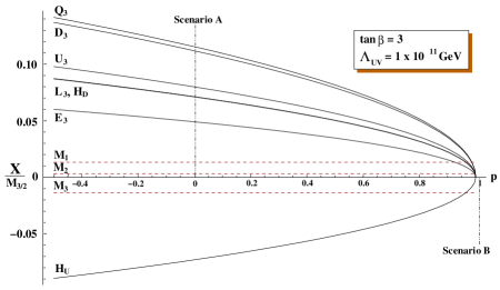
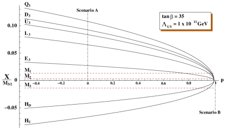
Figure 1: Soft Term Spectrum for Anomaly Dominated Scenario. Soft term magnitudes for third generation scalars, Higgs fields and gaugino masses are given as a function of universal PV parameter $p$ as a fraction of gravitino mass $m_{3/2}$. Scalar particles are generally much heavier than gauginos except for the limiting case of $p\rightarrow 1$.

One final aspect of these soft term patterns relevant to low energy phenomenology is the relative size of the scalar masses and A-terms. It is well known that for any generation of matter with non-negligible Yukawa couplings the relation

$$|A_{ijk}|^{2}\leq 3(M_{i}^{2}+M_{j}^{2}+M_{k}^{2}),$$ (3.9)

evaluated at the scale of supersymmetry breaking, is a good indicator that the minimum of the scalar potential will yield proper electroweak symmetry breaking: when the bound is not satisfied it is typical to develop minima away from the electroweak symmetry breaking point in a direction in which one of the scalars masses of a field carrying electric or color charge becomes negative. Since the “anomaly mediated” A-term and the scalar mass squared both have a single loop factor of $1/16\pi^{2}$ the condition (3.9) is generally satisfied. For example, in scenario (A) discussed above

$$(M_{i}^{2}+M_{j}^{2}+M_{k}^{2})=m_{3/2}A_{ijk},$$ (3.10)

and since $A_{ijk}$ is loop-suppressed relative to the gravitino mass, as seen from (3.6), this scenario is phenomenologically acceptable. Scenario (B) with its vanishing scalar masses at one loop is problematic, however, and the two loop contributions are relevant to the determination of its viability.

3.2 The O-II models

This class of orbifold models discussed in [1] has matter fields in the untwisted sector with weights $(n_{i}^{1},n_{i}^{2},n_{i}^{3})=(-1,0,0)$ $(0,-1,0)$ or $(0,0,-1)$. Then, taking for simplicity the same common value $T$ for the $T^{\alpha}$ fields, one obtains from (B.1):

$$M_{a}^{tot}=\frac{g_{a}^{2}(\mu)}{2\sqrt{3}}\overline{M}\left\{\frac{2}{\sqrt{3}}\cos\theta(t+\overline{t})G_{2}\left[\frac{\delta_{\rm GS}}{16\pi^{2}}+b_{a}^{0}\right]+\frac{2b_{a}^{0}}{\sqrt{3}}+\frac{\sin\theta}{k_{s\overline{s}}^{1/2}}\left[1+\frac{g_{s}^{2}}{16\pi^{2}}\left(C_{a}-\sum_{i}C_{a}^{i}\right)\right]\right\}.$$ (3.11)

The above form suggests a closer investigation of the relative magnitude of the contributions to gaugino masses arising from the dilaton sector (proportional to $\sin\theta$), the moduli sector (proportional to $\cos\theta$) and the anomaly-induced piece (independent of the Goldstino angle). As mentioned in the previous section, any tree level contribution (from the dilaton sector) will likely dominate the gaugino mass, particularly when the Green-Schwarz coefficient is smaller than $-3C_{E_{8}}$. The anomaly-induced piece is typically quite small and will only be relevant in the case of moduli domination ($\sin\theta=0$) with moduli stabilized very near their self-dual points and/or very small Green-Schwarz coefficient. This behavior is demonstrated for the case of the $U(1)_{Y}$ gaugino mass $M_{1}$ in Figure 2. We have taken $k=-\ln(S+\overline{S})$ and set $g_{s}^{2}=1/2$.

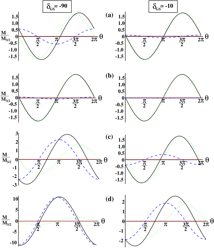
Figure 2: $U(1)_{Y}$ Gaugino Mass in the BIM O-II Model. Contributions to the value of $M_{1}$ from $F^{T}$ (dashed) and $F^{S}$ (dotted) as well as total $M_{1}$ (solid) are given as a function of Goldstino angle for two values of $\delta_{\rm GS}$ and four T-modulus vevs: $\left\langle{\rm Re}\;t\right\rangle=0.5$ (a), $\left\langle{\rm Re}\;t\right\rangle=0.9$ (b), $\left\langle{\rm Re}\;t\right\rangle=5$ (c), and $\left\langle{\rm Re}\;t\right\rangle=20$ (d). All values are given as a fraction of the gravitino mass $m_{3/2}$.

In Figure 3 we look at the relative sizes of the three gaugino mass terms for the case of moduli domination ($\theta=0$) and a mixed case ($\theta=\pi/3$) for real moduli vacuum values $\left\langle{\rm Re}\;t\right\rangle$ at a boundary scale of $\Lambda_{\rm UV}=2\times 10^{16}$ GeV. Note that there is always a particular value of the moduli vev such that a nearly degenerate gaugino mass spectrum is recovered. As $\cos\theta\rightarrow 0$ this value gets ever larger as we approach the limiting case in which the gaugino masses are independent of the value of $\left\langle{\rm Re}\ t\right\rangle$. At the GUT scale where $g_{2}^{2}\approx g_{1}^{2}\approx 1/2$ the difference in SU(2) and U(1) gaugino masses is given by

$$M_{2}-M_{1}\approx-\frac{m_{3/2}}{40\pi^{2}}\left\{7\left[1+\cos\theta\left(1-\frac{\pi}{3}{\rm Re}\ t\right)\right]+2\sqrt{3}\sin\theta\right\},$$ (3.12)

where we have used the fact that for ${\rm Re}\;t>1$, $\zeta(t)\approx-\pi/12$. For $\theta=0$ equation (3.12) indicates that $M_{1}=M_{2}$ at ${\rm Re}\;t\approx 6/\pi$ while for $\theta=\pi/3$ this occurs when ${\rm Re}\;t\approx 3.7$.

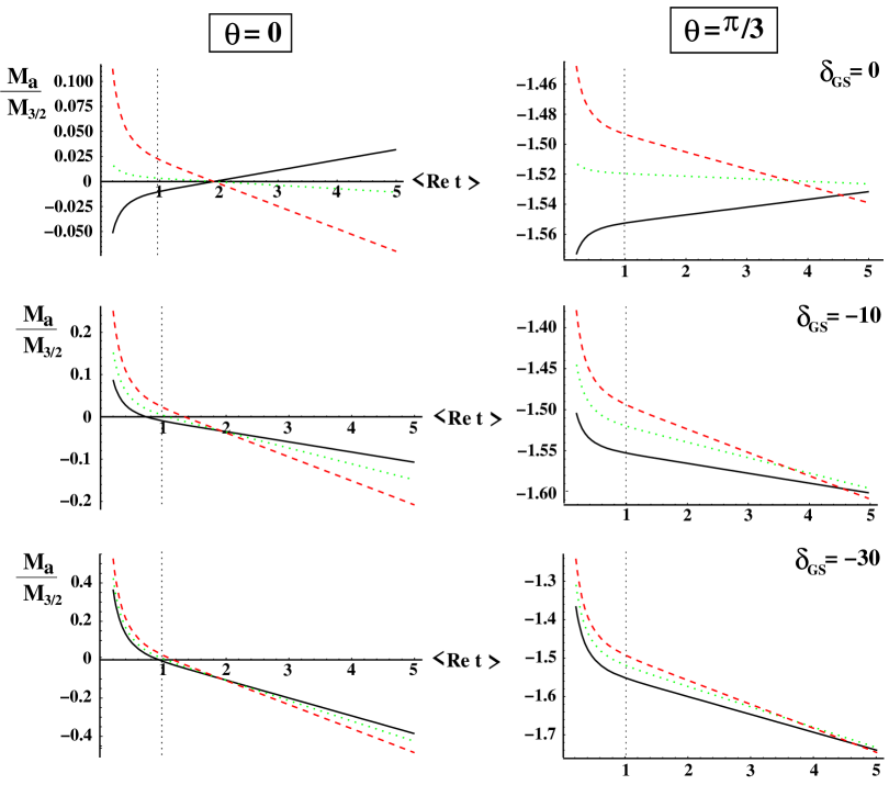
Figure 3: Relative Gaugino Masses vs. $\left\langle{\rm Re}\;t\right\rangle$ in the BIM O-II Model with $\Lambda_{\rm UV}=2\times 10^{16}$ GeV. Relative sizes of the three gaugino masses $M_{1}$ (dashed), $M_{2}$ (dotted) and $M_{3}$ (solid) are displayed as a function of $\left\langle{\rm Re}\;t\right\rangle$ for two values of the Goldstino angle $\theta$ and three representative values of $\delta_{\rm GS}$. The vertical dotted line at $\left\langle{\rm Re}\;t\right\rangle=1$ indicates the moduli self-dual point where gaugino masses become independent of $\delta_{\rm GS}$. When $\sin\theta=0$ this point represents the case of leading anomaly contributions discussed in Section 3.1. All masses are relative to the gravitino mass $m_{3/2}$.

When $\theta\not=0$ (3.12) implies that $|M_{2}|\geq|M_{1}|$ (the gaugino masses in this regime are negative) whenever

$${\rm Re}\ t\leq\frac{3}{\pi}\left\{\frac{2\sqrt{3}}{7}\tan\theta+\sec\theta+1\right\}.$$ (3.13)

In the case where $\theta=0$ so that there is no tree level contribution to gaugino masses we see from Figure 3 that $|M_{1}|\geq|M_{2}|$ in nearly all of the $\left\langle{\rm Re}\;t\right\rangle$ parameter space. This relationship between the boundary values of the SU(2) and U(1) gaugino masses is crucial to the low energy phenomenology of the model in that it determines whether the lightest neutralino is predominantly bino-like, predominantly wino-like or a mixed state. Thus a lightest neutralino with a significant wino content need not necessarily imply that supersymmetry breaking is due to pure anomaly mediation. We will return to this point when we investigate sample spectra in the next section.

The scale at which the soft masses emerge is particularly important: the largest contributions to gaugino masses generically arise from the tree level piece and the piece proportional to the Green-Schwarz coefficient $\delta_{\rm GS}$. These terms cancel in (3.12), however, when the difference is evaluated at the GUT scale. Thus the location of the crossover point is independent of the choice of $\delta_{\rm GS}$ in Figure 3.

An immediate consequence of the above is that measurement of the properties of the lightest neutralinos may reveal information on the nature of the scale of ultraviolet physics. In particular the region of parameter space for which the lightest neutralino is predominantly wino-like becomes increasingly small as the scale of supersymmetry breaking is lowered. This is illustrated in Figure 4 where we plot the ratio of gaugino masses $M_{1}/M_{2}$ for two different boundary scales: $\Lambda_{\rm UV}=2\times 10^{16}$ GeV and $\Lambda_{\rm UV}=1\times 10^{11}$ GeV, for which $g_{2}^{2}\approx(7/5)g_{1}^{2}$. As the gauge couplings run farther apart the shaded areas in which $M_{1}/M_{2}\geq 1$ (and hence where a wino-like lightest neutralino is possible) grow steadily smaller. When $\delta_{\rm GS}=0$ the ratio $M_{1}/M_{2}$ diminishes as the Goldstino angle $\theta$ increases until $M_{2}$ begins to approach its vanishing value and the ratio passes through a discontinuity before increasing rapidly as $\theta\rightarrow\pi$. When the Green-Schwarz coefficient $\delta_{\rm GS}$ is increased the location of this discontinuity, as indicated in Figure 4 by a heavy arrow, moves to smaller values of $\theta$.

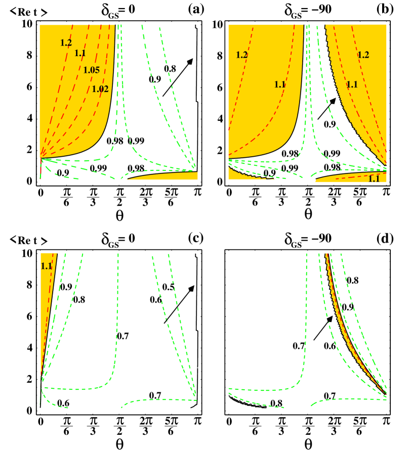
Figure 4: Ratio $M_{1}/M_{2}$ in BIM O-II Model. Contours of the absolute value of the ratio of U(1) to SU(2) gaugino masses are given for boundary scales of $\Lambda_{\rm UV}=2\times 10^{16}$ GeV for panels (a) and (b), and $\Lambda_{\rm UV}=1\times 10^{11}$ GeV for panels (c) and (d). The shaded area is the region of parameter space for which $|M_{1}|\geq|M_{2}|$. The arrow indicates the direction of smallest ratios as the discontinuity $M_{2}=0$ is approached. The contour $M_{1}=M_{2}$ is given by the heavy solid line.

The trilinear A-terms for these orbifold models are given by (B.3):

$$A^{tot}_{ijk} = \frac{\overline{M}}{\sqrt{3}}\left\{-\frac{\gamma_{i}}{\sqrt{3}}-\frac{\cos\theta}{\sqrt{3}}(t+\overline{t})G_{2}\left[\sum_{a}\gamma_{i}^{a}p_{ia}+\sum_{lm}\gamma_{i}^{lm}p_{lm}\right]+\frac{\sin\theta}{k_{s\overline{s}}^{1/2}}\left[-\frac{k_{s}}{3}+\sum_{lm}\gamma_{i}^{lm}\partial_{s}\ln({\tilde{\mu}}^{2}_{lm})\right.\right.$$ (3.14)

$$\left.\left.+\sum_{a}\gamma_{i}^{a}\left(\partial_{s}\ln({\tilde{\mu}}^{2}_{ia})+\frac{g_{a}^{2}}{2}\ln({\tilde{\mu}}^{2}_{ia})\right)-\ln\left[(t+\overline{t})|\eta(t)|^{4}\right]\left(\sum_{a}g_{a}^{2}\gamma_{i}^{a}p_{ia}-\sum_{lm}k_{s}\gamma_{i}^{lm}p_{lm}\right)\right]\right\}$$

$$+\rm{cyclic}(ijk),$$

where $p_{ia}=\sum_{\alpha}p_{ia}^{\alpha}$ and $p_{lm}=\sum_{\alpha}p_{lm}^{\alpha}$. For scenario (A), as defined by (2.38), this expression is particularly simple

$$A^{tot}_{ijk}=\frac{\overline{M}}{\sqrt{3}}\left\{\frac{\sin\theta}{k_{s\overline{s}}^{1/2}}\left[-\frac{k_{s}}{3}+\sum_{a}\gamma_{i}^{a}\frac{g_{a}^{2}}{2}\ln({\tilde{\mu}}^{2}_{ia}/\mu_{R}^{2})\right]-\frac{\gamma_{i}}{\sqrt{3}}\right\}+\rm{cyclic}(ijk).$$ (3.15)

It is worth noting that, with such a scenario for the PV metrics, this pattern for A-terms goes beyond the BIM O-II model. Any of the following conditions: (i) $\sum_{\alpha}(n^{\alpha}_{i}+n^{\alpha}_{j}+n^{\alpha}_{k}+1)=0$ with identical vacuum values for all T-moduli (as in the BIM O-II model), (ii) $\cos\theta=0$ (dilaton domination) or (iii) $G_{2}^{\alpha}=0$ (moduli stabilized at self-dual point), yields the A-terms given by (3.15) above.

By contrast, for scenario (B) defined by (2.39) the A-terms take the form

$$A^{tot}_{ijk} = \frac{\overline{M}}{\sqrt{3}}\left\{-\frac{\gamma_{i}}{\sqrt{3}}\left[1+\cos\theta(t+\overline{t})G_{2}\right]+\frac{\sin\theta}{k_{s\overline{s}}^{1/2}}\left[-\frac{k_{s}}{3}+\sum_{a}\frac{g_{a}^{2}}{2}\gamma_{i}^{a}(\ln(g_{a}^{2})-1)\right.\right.$$ (3.16)

$$\left.\left.-\ln\left[(t+\overline{t})|\eta(t)|^{4}\right]\left(\sum_{a}g_{a}^{2}\gamma_{i}^{a}-\sum_{lm}k_{s}\gamma_{i}^{lm}\right)\right]\right\}+\rm{cyclic}(ijk).$$

This scenario also allows for the recovery of an “anomaly mediated-like” result of A-terms proportional to anomalous dimensions in the moduli dominated limit ($\sin\theta=0$). Expression (3.16) differs from the situation in Section 3.1 in that for moduli domination this scenario can accommodate proper electroweak symmetry breaking provided the moduli are stabilized away from their self-dual points: in particular, using the fact that for ${\rm Re}\;t>1$, $\zeta(t)\approx-\pi/12$ we have $\left\langle(t+\overline{t})G_{2}\right\rangle\approx-1$ for $\left\langle t\right\rangle\approx 6/\pi\approx 2$ leading to $A\approx 0$ from (3.16).

The expressions for the bilinear B-terms are similar, but with added model dependence at the tree level involving the origin of bilinear terms in the Kähler potential or superpotential. For the case of scenario (A) the general form given in (B.4) yields

$$B^{tot}_{ij} = \frac{\overline{M}}{\sqrt{3}}\frac{\sin\theta}{k_{s\overline{s}}^{1/2}}\left[-k_{s}-\partial_{s}\ln\mu_{ij}+\sum_{a}\gamma_{i}^{a}\left(\frac{g_{a}^{2}}{2}\right)\ln({\tilde{\mu}}^{2}_{ia})\right.$$ (3.17)

$$\left.+\frac{\overline{M}}{6}\cos\theta\left[1-\sum_{\alpha}\partial_{t^{\alpha}}\ln\mu_{ij}\right]+\frac{\overline{M}}{3}\left(\frac{1}{2}-\gamma_{i}\right)\right]+(i\leftrightarrow j),$$

while for case (B) the corresponding expression is

$$B^{tot}_{ij} = \frac{\overline{M}}{\sqrt{3}}\frac{\sin\theta}{k_{s\overline{s}}^{1/2}}\left[-k_{s}-\partial_{s}\ln\mu_{ij}+\sum_{a}\gamma_{i}^{a}\frac{g_{a}^{2}}{2}\left(\ln(g_{a}^{2})-1\right)-\ln\left[(t+\overline{t})|\eta(t)|^{4}\right]\left(\sum_{a}\gamma_{i}^{a}g_{a}^{2}-\sum_{lm}\gamma_{i}^{lm}k_{s}\right)\right]$$ (3.18)

$$+\frac{\overline{M}}{3}\left(\frac{1}{2}-\gamma_{i}\right)+\frac{\overline{M}}{6}\cos\theta\left[1-\sum_{\alpha}\partial_{t^{\alpha}}\ln\mu_{ij}-2(t+\overline{t})G_{2}\gamma_{i}\right]+(i\leftrightarrow j).$$

Finally, the scalar masses in the BIM O-II model are found from equation (B.6) of Appendix B. Under the assumptions of scenario (A) this reduces to

$$(M_{i}^{tot})^{2} = |M|^{2}\left\{\frac{1}{9}\gamma_{i}+\frac{1}{k_{s\overline{s}}^{1/2}}\frac{\sin\theta}{3\sqrt{3}}\left[\sum_{a}\gamma_{i}^{a}g_{a}^{2}-\frac{1}{2}\sum_{jk}\gamma_{i}^{jk}(k_{s}+k_{\overline{s}})\right]+\frac{\sin^{2}\theta}{9}\left[1-\sum_{a}\gamma_{i}^{a}\ln({\tilde{\mu}}^{2}_{ia})\right.\right.$$ (3.19)

$$\left.\left.+2\sum_{jk}\gamma_{i}^{jk}\ln({\tilde{\mu}}^{2}_{jk})\right]+\frac{\sin^{2}\theta}{k_{s\overline{s}}}\left[-\frac{1}{4}\sum_{a}g_{a}^{4}\gamma_{i}^{a}\ln({\tilde{\mu}}^{2}_{ia})-\frac{1}{3}\sum_{jk}\gamma_{i}^{jk}\left(k_{s}k_{\overline{s}}+2k_{s\overline{s}}\right)\ln({\tilde{\mu}}^{2}_{jk})\right]\right\},$$

and for scenario (B) the scalar masses are given by

$$(M_{i}^{tot})^{2} = |M|^{2}\left\{\frac{1}{3\sqrt{3}}\frac{\sin\theta}{k_{s\overline{s}}^{1/2}}\left[1+\cos\theta(t+\overline{t})G_{2}\right]\left[\sum_{a}g_{a}^{2}\gamma_{i}^{a}-\frac{1}{2}\sum_{jk}\gamma_{i}^{jk}\left(k_{s}+k_{\overline{s}}\right)\right]\right.$$ (3.20)

$$\left.+\frac{\sin^{2}\theta}{9}\left[1+\gamma_{i}+\ln\left[(t+\overline{t})|\eta(t)|^{4}\right]\left(\sum_{a}\gamma_{i}^{a}-2\sum_{jk}\gamma_{i}^{jk}\right)-\sum_{a}\gamma_{i}^{a}\ln(g_{a}^{2})+2\sum_{jk}\gamma_{i}^{jk}\ln({\tilde{\mu}}^{2}_{jk})\right]\right.$$

$$\left.-\frac{\sin^{2}\theta}{k_{s\overline{s}}}\left[\sum_{a}\gamma_{i}^{a}\left(\frac{g_{a}^{4}}{4}\right)\left(\ln(g_{a}^{2})+\frac{5}{3}\right)+\frac{1}{3}\sum_{jk}\gamma_{i}^{jk}\left(k_{s}k_{\overline{s}}+2k_{s\overline{s}}\right)\ln({\tilde{\mu}}^{2}_{jk})\right.\right.$$

$$\left.\left.+\ln\left[(t+\overline{t})|\eta(t)|^{4}\right]\left(\sum_{a}\gamma_{i}^{a}\left(\frac{g_{a}^{4}}{4}\right)+\frac{1}{3}\sum_{jk}\gamma_{i}^{jk}k_{s}k_{\overline{s}}\right)\right]\right\}.$$

The pattern of soft supersymmetry breaking terms that arise in this orbifold model with uniform modular weights $n_{i}=-1$ and with the same Kähler metric for the $\Pi^{A}$ and the $\Phi^{A}$, as in scenario (2.39), will produce a low energy phenomenology very similar to that of the recently proposed “gaugino mediation” scenario [29] if the Green-Schwarz coefficient is sufficiently large, the supersymmetry breaking is moduli dominated and the moduli are stabilized at $\left\langle{\rm Re}\;t\right\rangle\approx 2$. Such a situation gives rise to exactly vanishing scalar masses and nearly vanishing A-terms and the gaugino masses in such a regime are very nearly universal, as can be seen from the lower panels of Figure 3. However, as the Green-Schwarz coefficient is reduced the gaugino masses become negligible at the point $\left\langle{\rm Re}\;t\right\rangle\approx 2$, eventually coming into conflict with direct search results at LEP and the Tevatron. Specific spectra for the O-II model will be presented with spectra for orbifold models with large threshold corrections, to which we now turn.

3.3 The O-I models

Models of this type were proposed with the goal of obtaining coupling constant unification at the string scale, as opposed to the extrapolated unification scale of $\Lambda_{\rm GUT}\approx 2\times 10^{16}$ GeV which is typically a factor of twenty or so lower than the string scale. This is achieved through large string threshold corrections and the requirement of both particular sets of modular weights for the massless fields and relatively large values of $\left\langle{\rm Re}\;t\right\rangle$ far from the self-dual points. Other solutions to this discrepancy of scales have been proposed since but because the O-I models have often been discussed in the literature we include them in the present discussion.

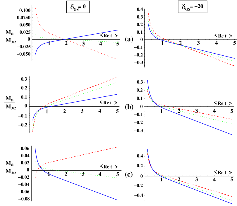
Figure 5: Relative Gaugino Masses in the BIM O-II and BIM O-I Models with $\theta=0$. Relative sizes of the three gaugino masses $M_{1}$ (dashed), $M_{2}$ (dotted) and $M_{3}$ (solid) are displayed as a function of $\left\langle{\rm Re}\;t\right\rangle$ for two values of the Green-Schwarz coefficient $\delta_{\rm GS}$ and $\Lambda_{\rm UV}=2\times 10^{16}$ GeV. The top panels (a) represent the BIM O-II model from Section 3.2, the middle panels (b) represent the BIM O-I model and the bottom panels (c) represent the Love & Stadler case from [31]. All masses are relative to the gravitino mass $m_{3/2}$.

To investigate the phenomenological consequences of such models we will assume a common vacuum value for all three moduli and take $\Theta_{\alpha}=1/\sqrt{3}$ as before. We shall investigate two scenarios: (A) the original “O-I” scenario of Brignole et al. [1] with modular weights $n_{Q}=n_{D}=-1$, $n_{U}=-2$, $n_{L}=n_{E}=-3$, $n_{H_{d}},n_{H_{u}}=-4$ and (B) a $Z_{3}\times Z_{6}$ compactification studied by Love and Stadler [31] with modular weights $n_{Q}=n_{D}=0$, $n_{U}=-2$, $n_{L}=-4$, $n_{E}=-1$, $n_{H_{d}}=n_{H_{u}}=-1$. In what follows let us assume that the soft terms emerge at a scale for which logarithms such as $\ln({\tilde{\mu}}^{2}_{ia})$ and $\ln({\tilde{\mu}}^{2}_{jk})$ are negligible and assume PV case (A) for simplicity. In this approximation the general expressions of Appendix B take a simplified form. The gaugino masses, given by

$$M_{a}^{tot} = g_{a}^{2}(\mu)\frac{\overline{M}}{3}\left\{b_{a}^{0}+\cos\theta(t+\overline{t})G_{2}\left[\frac{\delta_{\rm GS}}{16\pi^{2}}+b_{a}^{0}-\frac{1}{8\pi^{2}}\sum_{i}C_{a}^{i}(1+n_{i})\right]\right.$$ (3.21)

$$\left.+\frac{\sqrt{3}\sin\theta}{2k_{s\overline{s}}^{1/2}}\left[1+\frac{g_{s}^{2}}{16\pi^{2}}\left(C_{a}-\sum_{i}C_{a}^{i}\right)\right]\right\},$$

are displayed in Figure 5 with the value $\theta=0$ (where the impact of the differing modular weights is the greatest) for three models: the BIM O-II case of Section 3.2, the original BIM O-I case and the Love & Stadler case. The boundary scale is taken to be $\Lambda_{\rm UV}=2\times 10^{16}$ GeV. It is clear from Figure 5 that the modular weights of the matter fields play a crucial role in determining the gaugino mass spectrum provided the Green-Schwarz coefficient is sufficiently small. As this parameter is increased it will quickly come to dominate the other terms in (3.21).

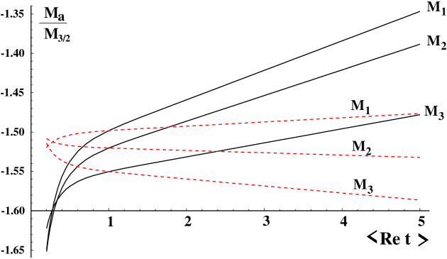
Figure 6: Relative Gaugino Masses in the BIM O-I Models with $\theta=\pi/3$ and $\delta_{\rm GS}=0$. Relative sizes of the three gaugino masses are displayed as a function of $\left\langle{\rm Re}\;t\right\rangle$ for the BIM O-I Model (solid) and the Love & Stadler Model (dashed) at $\Lambda_{\rm UV}=2\times 10^{16}$ GeV. All masses are relative to the gravitino mass $m_{3/2}$.

However, looking at the tree level expressions for the scalar masses (3.4) it is apparent that when $\cos\theta=1$ any field with a modular weight such that $n_{i}<-1$ will have a negative tree level scalar mass-squared, as was noted in [1]. Thus, to accommodate these large threshold models proper electroweak symmetry breaking (i.e. positive scalar mass-squareds) will generally require a Goldstino angle such that $\sin\theta$ is large and the tree level terms in (3.21) are dominant. Models with a viable low energy vacuum will therefore be models for which the impact of the matter fields’ modular weights on the gaugino spectrum is considerably muted. This is displayed in Figure 6 where gaugino masses in the BIM O-I model and the Love & Stadler model are displayed for $\theta=\pi/3$ and $\delta_{\rm GS}=0$. We see that in these realistic cases the differences in gaugino mass spectra between these models is small, making them hard to distinguish experimentally.

The trilinear A-terms for scenario (A) are

$$A^{tot}_{ijk}=\frac{\overline{M}}{3}\left\{-\gamma_{i}+\frac{\cos\theta}{3}(t+\overline{t})G_{2}(n_{i}+n_{j}+n_{k}+3)-\frac{\sin\theta}{\sqrt{3}}\frac{k_{s}}{k_{s\overline{s}}^{1/2}}\right\}+\rm{cyclic}(ijk),$$ (3.22)

and the scalar masses are determined from

$$(M_{i}^{tot})^{2} = \frac{|M|^{2}}{9}\left\{(1+\gamma_{i})+\cos\theta(t+\overline{t})G_{2}\sum_{jk}\gamma_{i}^{jk}(n_{i}+n_{j}+n_{k}+3)+n_{i}\cos^{2}\theta\right.$$ (3.23)

$$\left.+\frac{\sqrt{3}\sin\theta}{k_{s\overline{s}}^{1/2}}\left(\sum_{a}\gamma_{i}^{a}g_{a}^{2}-\frac{1}{2}\sum_{jk}\gamma_{i}^{jk}\left(k_{s}+k_{\overline{s}}\right)\right)\right\},$$

With these expressions we are now in a position to compare the typical spectra of these O-I large threshold models with the models of Section 3.1 and Section 3.2.

Model	Anomaly (3.1)	BIM O-II (3.2)					BIM O-I (3.3)	L&S (3.3) [31]
$\theta$	0	0	0	0	0	$\pi/3$	$\pi/3$	$\pi/3$
$\delta_{\rm GS}$	N/A	0	0	0	-90	-90	-90	-90
$\left\langle{\rm Re}\;t\right\rangle$	1	$6/\pi$	5	20	$6/\pi$	$6/\pi$	16	14.5
$m_{3/2}$	$1.9\times 10^{4}$	$1.9\times 10^{4}$	$1.6\times 10^{4}$	4500	1600	450	150	150
$m_{\tilde{N_{1}}}$	51.81	0.32	152.53	248.97	332	313	287	297
$m_{\tilde{N_{2}}}$	168	3.7	462	759	615	599	557	581
$\tilde{B}$ %	0.01	80.9	0.001	0.001	99.9	99.9	99.9	99.9
$\tilde{W_{3}}$ %	99.7	19.1	99.7	99.7	0.001	0.001	0.001	0.001
$m_{\tilde{\chi_{1}}^{\pm}}$	51.83	3.1	152.55	249.00	615	599	557	581
$m_{\tilde{g}}$	623	3.6	1468	2245	2156	2164	2106	2128
$m_{h}$	114	114	114	114	114	114	114	114
$m_{A}$	2237	2217	1992	1357	1447	1387	1810	1568
$m_{\tilde{t}_{R}}$	860	796	1142	1597	1521	1610	1373	1532
$m_{\tilde{t}_{L}}$	1842	1810	1818	1820	1804	1866	1709	1793
$m_{\tilde{b}_{R}}$	1805	1765	1802	1769	1782	1847	1701	1773
$m_{\tilde{b}_{L}}$	1810	1770	1824	1908	1883	1945	1881	1871
$m_{\tilde{\tau}_{R}}$	1191	1180	1076	514	329	302	198	290
$m_{\tilde{\tau}_{L}}$	1193	1182	1078	515	330	303	281	301
$A_{\rm top}$	391	71	-815	-1423	1696	1541	560	1607
$A_{\rm bot}$	973	463	-999	-1827	2819	2200	-405	4650
$A_{\rm tau}$	220	273	376	305	466	-184	-7417	-2734
$\mu$	1617	1592	1501	1281	1341	1302	1577	1297

Table 2: Sample Spectra (in GeV) for Typical Models of Sections 3.1, 3.2 and 3.3. All cases are for PV scenario (A), $\tan\beta=3$ and $\Lambda_{\rm UV}=2\times 10^{16}$ GeV ($\tilde{B}$ % and $\tilde{W_{3}}$ % represent the content of the lightest neutralino in per cents). The first O-II case considered, while clearly ruled out experimentally, is presented as an illustrative example.

In Tables 2 and 3 we give some representative sample spectra for Pauli-Villars scenario (A) defined by (2.38) and $\tan\beta=3$ and $\tan\beta=10$, respectively. The spectra for scenario (B) are very similar and these values vary only minimally when $\Lambda_{\rm UV}$ is varied. To obtain these spectra at the electroweak scale the renormalization group equations (RGEs) were run from the boundary scale to the electroweak scale. All gauge and Yukawa couplings as well as gaugino masses and A-terms were run with one loop RGEs while scalar masses were run at two loops to capture the possible effects of heavy scalars on the evolution of third generation squarks and sleptons. We chose to keep only the top, bottom and tau Yukawas and the corresponding A-terms. The gravitino mass has been scaled in each case to obtain a Higgs mass of 114 GeV, which can be considered either as a limiting case or as an experimental requirement, depending on what happens next at LEP.

At the electroweak scale the one loop corrected effective potential $V_{\rm 1-loop}=V_{\rm tree}+\Delta V_{\rm rad}$ is computed and the effective $\mu$-term $\bar{\mu}$ is calculated

$${\bar{\mu}}^{2}=\frac{\left(m_{H_{d}}^{2}+\delta m_{H_{d}}^{2}\right)-\left(m_{H_{u}}^{2}+\delta m_{H_{u}}^{2}\right)\tan{\beta}}{\tan^{2}{\beta}-1}-\frac{1}{2}M_{Z}^{2}.$$ (3.24)

In equation (3.24) the quantities $\delta m_{H_{u}}$ and $\delta m_{H_{d}}$ are the second derivatives of the radiative corrections $\Delta V_{\rm rad}$ with respect to the up-type and down-type Higgs scalar fields, respectively. These corrections include the effects of all third generation particles. If the right hand side of equation (3.24) is positive then there exists some initial value of $\mu$ at the condensation scale which results in correct electroweak symmetry breaking with $M_{Z}=91.187$ GeV.

Note that the gravitino mass varies greatly over the models considered in Tables 2 and 3. For the anomaly case (which is equivalent to the BIM O-II model with $\sin\theta=0$ and $\left\langle{\rm Re}\;t\right\rangle=1$) there is a large hierarchy between scalars and gauginos, as noted in Section 3.1, which necessitates a large value of the gravitino mass to yield neutralinos with masses near the current LEP limits. Having normalized our scales to yield Higgs masses of 114 GeV we find chargino masses (for PV scenario (A) and thus $p=0$ in Figure 1) below the recently reported bounds of $m_{\chi^{\pm}}\geq 86.1$ GeV for the case of a chargino which is nearly degenerate with a wino-like lightest neutralino [32]. As the PV scenario assumed is modified, however, this relation between the chargino mass and Higgs mass varies. In particular as the value of $p$ approaches larger, positive values the gauginos steadily become heavier for a fixed Higgs mass, eventually satisfying the experimental constraints. For the large threshold models, by contrast, the large values of $\left\langle{\rm Re}\;t\right\rangle$ necessary to ensure gauge coupling unification at the string scale make the gauginos typically heavier than the gravitino at the boundary scale $\Lambda_{\rm UV}$, due to the large value of $(t+\overline{t})G_{2}$, and have a smaller degree of hierarchy between gauginos and scalars.

Model	Anomaly (3.1)	BIM O-II (3.2)					BIM O-I (3.3)	L&S (3.3) [31]
$\theta$	0	0	0	0	0	$\pi/3$	$\pi/3$	$\pi/3$
$\delta_{\rm GS}$	N/A	0	0	0	-90	-90	-90	-90
$\left\langle{\rm Re}\;t\right\rangle$	1	$6/\pi$	5	20	$6/\pi$	$6/\pi$	16	14.5
$m_{3/2}$	8000	8000	6500	1800	1200	200	N/A	N/A
$m_{\tilde{N_{1}}}$	20.20	0.17	62.11	98.72	139	129
$m_{\tilde{N_{2}}}$	70	3.11	187	301	260	244
$\tilde{B}$ %	0.08	79.2	0.002	$1.9\times 10^{-7}$	99.3	99.1
$\tilde{W_{3}}$ %	98.0	20.8	97.8	97.4	0.001	0.002
$m_{\tilde{\chi_{1}}^{\pm}}$	20.21	2.5	62.14	98.75	260	244
$m_{\tilde{g}}$	280	1.85	644	978	1020	979
$m_{h}$	114	114	114	114	114	114
$m_{A}$	797	790	689	485	560	497
$m_{\tilde{t}_{R}}$	449	427	527	658	663	667
$m_{\tilde{t}_{L}}$	797	782	774	806	849	819
$m_{\tilde{b}_{R}}$	739	720	727	737	792	771
$m_{\tilde{b}_{L}}$	763	744	753	799	838	812
$m_{\tilde{\tau}_{R}}$	493	490	431	206	147	121
$m_{\tilde{\tau}_{L}}$	503	499	440	211	156	132
$A_{\rm top}$	190	47	-336	-596	796	668
$A_{\rm bot}$	398	187	-403	-858	1223	893
$A_{\rm tau}$	83	108	153	130	190	100
$\mu$	578	565	529	495	559	499

Table 3: Sample Spectra (in GeV) for Typical Models of Sections 3.1, 3.2 and 3.3. The same as in Table 2 but for $\tan\beta=10$. Neither of the large threshold models are viable at this value of $\tan\beta$.

The O-II models can interpolate between these two extremes. When $\theta=0$ and $\delta_{\rm GS}=0$ the pattern of physical masses shows the anomaly mediated feature of a wino-like LSP. As the value of $\left\langle{\rm Re}\;t\right\rangle$ increases from $\left\langle{\rm Re}\;t\right\rangle=1$ (the pure anomaly mediated case) it first passes through the experimentally excluded values where $\left\langle{\rm Re}\;t\right\rangle\approx 6/\pi$ and the gaugino masses are nearly zero. Thereafter the hierarchy between gauginos and scalars steadily decreases until the spectra of masses is very similar to that of the more typical supergravity spectra to the right of Table 2. However, as mentioned at the end of the previous section the feature of a wino-like LSP persists. Once $\theta\not=0$ and/or $\delta_{\rm GS}\not=0$ the pattern of soft terms immediately becomes relatively insensitive to the value of $\left\langle{\rm Re}\;t\right\rangle$ and the LSP once again becomes predominantly bino-like.

The models with large threshold corrections also tend to have very light staus. In fact, as the value of $\tan\beta$ increases the stau mass $m_{\tilde{\tau}_{R}}$ eventually becomes negative. The limiting value of $\tan\beta$ for which these models are phenomenologically viable depends slightly on the value of $\delta_{\rm GS}$: for $\theta=\pi/3$ the model of Love & Stadler requires $\tan\beta<9.1$ when $\delta_{\rm GS}=-90$ and $\tan\beta<4.8$ when $\delta_{\rm GS}=0$, while the original BIM O-I model requires $\tan\beta<3.1$ when $\delta_{\rm GS}=-90$ and is not allowed at all for $\delta_{\rm GS}=0$. This is reflected in the empty columns in Table 3. This problem is slightly ameliorated when the Goldstino angle is increased. For $\theta=2\pi/5$, for example, the model of Love & Stadler requires $\tan\beta<12.7$ when $\delta_{\rm GS}=-90$ and $\tan\beta<9.6$ when $\delta_{\rm GS}=0$, while the original BIM O-I model requires $\tan\beta<4.9$ when $\delta_{\rm GS}=-90$ and $\tan\beta<2.1$ when $\delta_{\rm GS}=0$.

The pattern of masses exhibited in Tables 2 and 3 suggests that the hierarchy between gauginos and scalars in any potential observation of supersymmetry will be a key to understanding the nature of the underlying physics giving rise to supersymmetry breaking. The observation of a lightest neutralino with significant wino content will not be enough to distinguish between the pure anomaly mediated cases and the BIM O-II type models but will indicate that supersymmetry breaking is moduli dominated within this class of models. The presence of a large hierarchy between scalars and gauginos and large mixing in the stop sector will point towards moduli stabilized at or near their self-dual values, while the absence of such effects would suggest the moduli are stabilized far from these values.

3.4 The BGW model

In this section we give the soft supersymmetry breaking parameters for the model of Ref. [23], with an explicit mechanism for supersymmetry breaking through gaugino condensation in a hidden sector, and dilaton stabilization by nonperturbative string effects. An effective Lagrangian below the scale $\mu_{c}$ of hidden gaugino condensation is constructed [19, 20] by replacing the linear multiplet $L$ in (2.16) by a vector multiplet $V$ whose components includes those of $L$ and of a chiral multiplet $U$ and its conjugate $\bar{U}$. The superfield $U$ satisfies the same equations as the composite chiral superfield $\hat{U}=W^{\alpha}W_{\alpha}$ constructed from the Yang-Mills superfield strength, and is interpreted as the lightest chiral superfield bound state of the effective theory below the condensation scale $\mu_{c}=|u|^{1\over 3},$ where $u=U|$ is the scalar component of the chiral supermultiplet $U$. An effective potential for the gaugino condensates $U$, as well as matter condensates $\Pi$ that are present if there is elementary matter charged under the confined gauge group, is constructed by field theory anomaly matching. Once the massive ($m\geq\mu_{c}$) composite degrees of freedom are integrated out, this generates a potential for the dilaton and moduli.

The gaugino masses were given in [13]. In the notation adopted here they take the form

$$M_{a}={g^{2}_{a}(\mu)\over 2}F^{S}+M^{(1)}_{a},$$ (3.25)

where $M^{(1)}_{a}$ is given in (2.22). The A-terms, squared soft scalar masses and B-terms are given by (2.35), (2.56)–(2.57) and (2.47) respectively, with (see Appendix A)

$$M={1\over 2}b_{+}^{0}u=-3m_{3/2},\quad F^{S}=-{1\over 4}K^{-1}_{S{\bar{S}}}\left(1+{g^{2}_{s}\over 3}b_{+}^{0}\right)\bar{u},\quad K_{S}=-{1\over 2}g^{2}_{s},$$ (3.26)

where $g^{2}_{s}$ is defined in (2.23) and $b_{+}^{0}$ is the beta function coefficient, Eq. (2.15), of the condensing gauge group ${\cal G}_{+}$. The model of Ref. [23] is explicitly modular invariant, so the moduli are stabilized at their self-dual points with $\left\langle F^{\alpha}\right\rangle=0$, and supersymmetry breaking is dilaton dominated. Then [23]

$$A^{(0)}_{ijk}={g^{2}_{s}\over 2}F^{S},\quad M^{(0)}_{i}={1\over 3}|M|=|m_{3/2}|.$$ (3.27)

Vanishing of the vacuum energy (2.4) now requires

$$K_{S{\bar{S}}}|F^{S}|^{2}={1\over 3}|M^{2}|,\quad K^{-1}_{S{\bar{S}}}={(2b_{+}^{0})^{2}\over 3(1+{1\over 3}g^{2}_{s}b_{+}^{0})^{2}},\quad\left|{F^{S}\over M}\right|={2b_{+}^{0}\over 3(1+{1\over 3}g^{2}_{s}b_{+}^{0})},$$ (3.28)

If $b_{+}^{0}\ll 1$ the tree level A-terms and gaugino masses are suppressed relative to the the gravitino mass, whereas the scalar masses and B-terms, $B^{(0)}_{ij}\approx-m_{3/2}$, are not. Therefore one loop corrections can be neglected for the latter, but may be important for the former. It is clear from (2.22) and (2.35) that the dominant one loop corrections in this case are just the “anomaly mediated” terms found in [2, 3]:

$$M_{a} \approx M^{(0)}_{a}+g_{a}(\mu^{2}){b^{0}_{a}\over 3}\bar{M}=g_{a}(\mu^{2})m_{3/2}\left({b_{+}^{0}\over 1+{1\over 3}g_{s}^{2}b_{+}^{0}}-b^{0}_{a}\right),$$

$$A_{ijk} \approx A^{(0)}_{ijk}-{1\over 3}M\left(\gamma_{i}+\gamma_{j}+\gamma_{k}\right)=m_{3/2}\left({g^{2}_{s}b_{+}^{0}\over 1+{1\over 3}g_{s}^{2}b_{+}^{0}}+\gamma_{i}+\gamma_{j}+\gamma_{k}\right).$$ (3.29)

This model was analyzed in detail in [30]. Over most of the allowed parameter space, $.1\geq b_{+}^{0}\gg b^{0}_{a}$, the tree contributions dominate. However there is a small region of parameter space with a sufficiently small value of $b_{+}^{0}$ that the gaugino masses and A-terms are similar to those in an “anomaly mediated” scenario [2, 3, 16].

Using the expressions in Appendix B, together with (3.26) and (3.28) the pattern of soft supersymmetry breaking terms can be obtained as a function of the condensing group beta function coefficient $b_{+}^{0}$ and the modular weights of the fields with $\left\langle{\rm Re}\;t\right\rangle=1$ or $\left\langle{\rm Re}\;t\right\rangle=e^{i\pi/6}$ and $\sin\theta=1$. The condensation scale in these models is typically of the order of $1\times 10^{14}$ GeV and we take this to be the boundary condition scale $\Lambda_{\rm UV}$ in what follows. In Figure 7 the gaugino masses are displayed as a function $b_{+}^{0}$ as a fraction of the gravitino mass. In [30] it was shown that for weak coupling at the string scale ($g_{s}^{2}\approx 1/2$) a reasonable scale of supersymmetry breaking (i.e. gravitino masses less than 10 TeV) generally requires $b_{+}^{0}\leq 0.085$. The region with gravitino mass larger than $10$ TeV is shaded in Figure 7. Also indicated in Figure 7 is a benchmark scenario consisting of an $E_{6}$ gaugino condensate in the hidden sector together with 9 27s of matter and having a beta function coefficient of $b_{+}^{0}=0.038$.

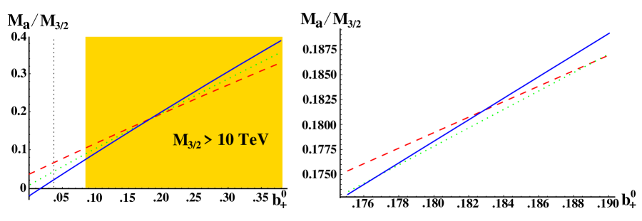
Figure 7: Gaugino Masses in the BGW Model. Gaugino masses $M_{1}$ (dashed), $M_{2}$ (dotted) and $M_{3}$ (solid) are given at a scale $\Lambda_{\rm UV}=1\times 10^{14}$ GeV as a function of the condensing group beta function coefficient $b_{+}^{0}$. The vertical dotted line in the left panel is the case of $E_{6}$ condensation in the hidden sector with 9 27s of hidden sector matter studied in [30]. The right panel focuses on the region where the three masses are approximately unified.

The spectrum of gaugino masses will typically be similar to that of the “anomaly-mediated” cases with $M_{1}\geq M_{2}$ and a lightest neutralino with substantial wino-like content provided $b_{+}^{0}\leq 0.19$. The location of the approximate unification of gaugino masses near this value of $b_{+}^{0}$ is expanded in the right panel of Figure 7.

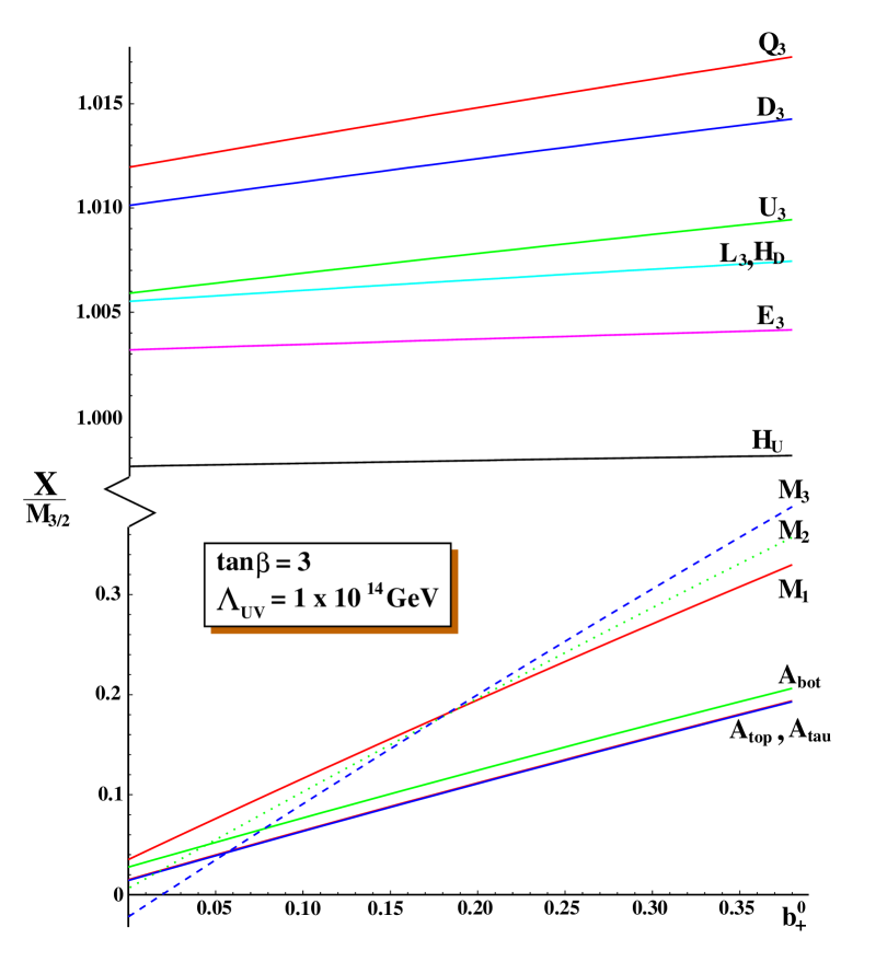
Figure 8: Spectrum of Soft Supersymmetry Breaking Terms in BGW Model. All values are given relative to the gravitino mass $m_{3/2}$ at a scale $\Lambda_{\rm UV}=1\times 10^{14}$ GeV as a function of the condensing group beta function coefficient $b_{+}^{0}$.

In Figure 8 we plot the relative sizes of all third generation scalar masses and A-terms, Higgs masses and gaugino masses as a fraction of the gravitino mass for $\tan\beta=3$, assuming $n_{i}=-1$ for all fields. As was the case in Sections 3.1-3.3, the gauginos are typically an order of magnitude smaller than scalars (note the change in vertical scale in Figure 8). Despite this hierarchy, this model was shown in [30] to give rise to acceptable low energy phenomenology provided $\tan\beta$ was in the low to moderate range. Figure 8 displays an important feature of the always-present one loop contributions arising from the conformal anomaly: when tree level scalar masses are present and universal the non-universality arising from the anomaly pieces is negligible (here averaging less than a 1% correction). However, the corrections to the gaugino masses may significantly alter the gaugino spectrum provided the tree level contributions are absent or suppressed, as in the BGW model considered here. Neglecting these one loop anomaly-induced contributions to soft terms is an approximation whose validity needs to be assessed on a model-by-model basis.

3.5 Matter couplings to the Green-Schwarz term

So far we have assumed the Green-Schwarz function $V_{GS}$ depends only on the moduli, that is, we set $p_{i}=0$ in (2.17). Only the moduli couplings in this term are known from string loop calculations [7, 8] and they are proportional to the Kähler potential for the moduli. It is possible that the GS function is proportional to the full Kälher potential, in which case $p_{i}=p=-\delta_{GS}/24\pi^{2}$, or that it is proportional to the untwisted Kähler potential, i.e. to the logarithm of the determinant of the metric in the six dimensional compact space. In this last case we would have $p_{i}=p$ for untwisted matter and $p_{i}=0$ for twisted matter. The presence of these terms modifies the soft parameters if $F^{S}\neq 0$.

One effect of $p_{i}\neq 0$ is a modification [33] of the “effective” matter Kähler potential (2.9):

$$\kappa_{i} \to \left(1+{1\over 2}g_{s}p_{i}\right)\kappa_{i}.$$ (3.30)

The potential can still be written in the form given in (A.8) of the appendix with the replacement $K_{N\bar{N}}\to\hat{K}_{N\bar{N}}=K_{N\bar{N}}+{1\over 2}g_{s}(V_{GS})_{N\bar{N}}$. However the effective metric is not Kähler in this formulation. In addition $F^{N}$ does not take the usual form (2.1): $F^{N}=-e^{-K/2}W^{-1}\hat{K}^{N\bar{N}}\partial_{\bar{N}}\left(e^{K}W\overline{W}\right)$, which reduces to (2.1) when $W$ is holomorphic. This is not the case in the linear multiplet formulation for the dilaton that we are using here because of the way the GS term enters in the dilaton potential, as described in Appendix A. For these reasons Eqs. (2.27), (2.54) and (2.45) do not generally apply if $F^{S}\neq 0$; the $p_{i}$-terms in these parameters depend on the specifics of the model for generating a potential for the dilaton. The PV metrics (2.33) are similarly modified:

$$\kappa^{\Phi}_{i}\to\left(1+{1\over 2}g_{s}p_{i}\right)\kappa^{\Phi}_{i},\quad\hat{\kappa}^{\Phi}_{i}\to\left(1+{1\over 2}g_{s}p_{i}\right)^{-1}\hat{\kappa}^{\Phi}_{i},$$ (3.31)

as are the soft parameters in the PV potential. These give additional one loop contributions, which can be important for gaugino masses which have no tree level contribution from $p_{i}\neq 0$.

Here we give the results only for the explicit dilaton dominated supersymmetrybreaking model of the previous subsection:

$$\Delta A_{ijk} \approx \Delta A_{ijk}^{(0)}=-{p_{i}\left(3+g^{2}_{s}b_{+}^{0}\right)\over 2b_{+}^{0}\left(1+{1\over 2}g_{s}p_{i}\right)}m_{3/2}+(i\to j)+(j\to k),$$

$$\Delta B_{ij} \approx \Delta B_{ij}^{(0)}-{p_{i}\left(3+g^{2}_{s}b_{+}^{0}\right)\over 2b_{+}^{0}\left(1+{1\over 2}g_{s}p_{i}\right)}m_{3/2}+(i\to j),$$

$$\Delta M_{a} \approx \Delta M_{a}^{(1)}={g^{2}(\mu)\over 8\pi^{2}}\sum_{i}{C^{i}_{a}p_{i}\left(3+g^{2}_{s}b_{+}^{0}\right)\over 2b_{+}^{0}\left(1+{1\over 2}g^{2}_{s}p_{i}\right)}m_{3/2}.$$ (3.32)

Note that in this special case the above results can in fact be obtained from the general formulae (2.22), (2.27) and (2.45):

$$\Delta A^{(0)}_{ijk} = -F^{S}K_{S{\bar{S}}}{p_{i}\over 1+{1\over 2}g_{s}p_{i}}+(i\to j)+(j\to k),$$

$$\Delta B^{(0)}_{ij} = -F^{S}K_{S{\bar{S}}}{p_{i}\over 1+{1\over 2}g_{s}p_{i}}+(i\to j),$$

$$\Delta M^{(1)}_{a} = {g^{2}(\mu)\over 8\pi^{2}}F^{S}K_{S{\bar{S}}}\sum_{i}{p_{i}C^{i}_{a}\over 1+{1\over 2}g^{2}_{s}p_{i}},$$ (3.33)

since it follows from (3.30) that

$$F^{n}\partial_{n}\ln\kappa_{i} \to F^{n}\partial_{n}\ln\kappa_{i}-F^{S}K_{S{\bar{S}}}{p_{i}\over 1+{1\over 2}g_{s}p_{i}},$$ (3.34)

where we used the relation

$${\partial g_{s}\over\partial s}=2{\partial\ell\over\partial x}=-K_{S{\bar{S}}},$$ (3.35)

given in Appendix A. However (2.54) does not apply even in this case; the tree level scalar masses in this model have been given in [23]:

$$|M^{(0)}_{i}|={1\over b_{+}^{0}}\left|{3p_{i}-2b_{+}^{0}\over 2+p_{i}g^{2}_{s}}m_{3/2}\right|.$$ (3.36)

The results (3.32) then follow from (3.28). We see a considerable enhancement of all these parameters if $p_{i}=p>>b_{+}^{0}$. Under the assumption that $-\delta_{GS}$ takes its maximum value of 90, the only viable scenario with some $p_{i}=p$ found in [30] is for $p_{H_{u,d}}=0$ and $p_{i}=p$ for all three generations of squarks and sleptons.

4 Conclusion

To conclude, let us first stress that even though we have been studying specific classes of superstring models, the types of spectra that we obtained and discussed appear to be quite generic. For example, scenarios from models with extra dimensions tend to give spectra which can be related to one or another type considered here, whether it is the model of Randall and Sundrum [2], or models of gaugino mediation [29].

In particular, soft terms that are proportional to beta function coefficients and anomalous dimensions can be realized in a variety of ways in string-derived supergravity. The case that is generally referred to as “anomaly mediation” is just one limiting value in a continuum of such models. The importance of these anomaly-induced terms depends on the absence or suppression of tree level contributions to the soft supersymmetry breaking parameters and on the assumptions made regarding the underlying theory when regulating the effective supergravity theory.

Once supersymmetry is discovered, the central issue will be to unravel the mechanism of supersymmetry breaking. The search strategy will be of the most value if it is based on large classes of different models, not just on a single “minimal” model. The models studied above tend to show that a possible strategy could be based on three steps:

(i) identifying gaugino masses (the least model dependent aspect of these theories) and the nature of the LSP,

(ii) identifying where (approximately) the bulk of the scalar masses lie and whether there is an order of magnitude between gaugino and scalar masses,

(iii) then using the detail of the scalar masses, in particular the mixing in the stop sector and the degree of non-universality, to disentangle the possible scenarios.

Observation of non-universal supersymmetric parameters obeying the relations described in Sections 3.1-3.4 will likely shed light on the scale of supersymmetry breaking, the nature of the fields responsible for this breaking and the origin of the $\mu$-term, if not the properties of the underlying superstring theory itself.

Acknowledgements

We thank Joel Giedt for discussions. P.B. thanks the Theory Group of LBNL for its generous hospitality and the participants of the GDR Supersymmetry working group on non-universalities, especially Laurent Duflot and Jean-François Grivaz, for discussions. B.N. would like to thank the Laboratoire de Physique Théorique at the Université Paris-Sud where part of this work was completed. This work was supported in part by the Director, Office of Science, Office of Basic Energy Services, of the U.S. Department of Energy under Contract DE-AC03-76SF00098 and in part by the National Science Foundation under grants PHY-95-14797 and INT-9910077.

Appendix

A. The linear multiplet formalism for the dilaton

In this paper we have presented the soft supersymmetry breaking parameters in terms of the various auxiliary fields of supergravity. In order to adhere as closely as possible to the notation of [1], we used expressions of the form obtained in the standard chiral formulation of supergravity. In the context of string theory, the dilaton $\ell$ appears as the scalar component of a linear multiplet $L$. The chiral multiplet formulation can be recovered by a duality transformation, at least at the classical level. However the linear multiplet formulation provides a simpler implementation of the Green-Schwarz anomaly cancellation mechanism and a better framework for constructing an effective Lagrangian for gaugino condensation. The effective theory of [23] made explicit use of the linear multiplet formalism. In this appendix we show the correspondence between various terms in the component Lagrangian of the linear formalism and of the expressions given in the text. We also show how explicit cancellations among the light loop (anomaly) contribution, the GS term and the string threshold corrections result in the final expression (2.22) for the one loop gaugino mass. These cancellations are most readily displayed in the linear multiplet formalism. Finally, we will display corrections to the soft parameters in the scalar potential that are present if the dilaton and moduli sectors both contribute substantially to supersymmetry breaking.

In the presence of a (nonperturbatively induced) potential for the dilaton, the tree level scalar Lagrangian takes the form (dropping gauge charged matter)

$${\cal L}_{\rm scalar}=-\sum_{\alpha}{\partial_{m}t^{\alpha}\partial^{m}\bar{t}^{\alpha}\over(t^{\alpha}+\bar{t}^{\alpha})^{2}}-{k^{\prime}(\ell)\over 4\ell}\partial_{m}\ell\partial^{m}\ell-{\ell\over k^{\prime}(\ell)}\partial_{m}a\partial^{m}a-V,$$ (A.1)

where the axion $a$ is related to the two-form $b_{mn}$ of the linear multiplet by a duality transformation:

$${1\over 2}\epsilon^{mnpq}\partial_{n}b_{pq}=-{2\ell\over k^{\prime}(\ell)}\partial^{m}a.$$ (A.2)

The potential $V$ can be written in the form

$$V = \sum_{\alpha}{1\over(t^{\alpha}+t^{\alpha})^{2}}F^{\alpha}\bar{F}^{\alpha}+{\ell\over k^{\prime}(\ell)}F^{2}-{1\over 3}M\bar{M},$$

$$F = {k^{\prime}(\ell)\over 4\ell}f(\ell,t^{\alpha},z^{i}),$$ (A.3)

where $f(\ell,t^{\alpha},z^{i})$ is a complex but nonholomorphic function of the scalar fields. For example in the model of [23],

$$f(\ell,t^{\alpha},z^{i})=-\sum_{a}(1+\ell b_{a})\bar{u}_{a}\approx-(1+\ell b_{+})\bar{u}_{+},$$ (A.4)

where $\bar{u}_{a}(\ell,t^{\alpha},z^{i})$ is the value of the gaugino condensate for a hidden gauge group ${\cal G}_{a}$ with beta function coefficient $b_{a}=\left(C_{a}-{1\over 3}\sum_{i}C_{a}^{i}\right)/8\pi^{2}=2b_{a}^{0}/3$; the function (A.4) is dominated by the condensate $\bar{u}_{+}$ with the largest beta function coefficient $b_{+}$.

To cast this result in a form resembling the standard chiral formulation we introduce the variable $x(\ell)=2g^{-2}(M_{s})$, which is twice the inverse squared gauge couplng (2.23). It is related to the dilaton Kähler potential $k$ by the differential equation [5]

$$k^{\prime}(\ell)=-\ell x^{\prime}(\ell),\quad\partial\ell=-{\ell\over k^{\prime}(\ell)}\partial x,$$ (A.5)

giving

$${\partial k(x)\over\partial x}=k^{\prime}(\ell){\partial\ell\over\partial x}=-\ell,\quad{\partial^{2}k(x)\over\partial x^{2}}=-{\partial\ell\over\partial x}={\ell\over k^{\prime}(\ell)},$$

$${k^{\prime}(\ell)\over 4\ell}\partial_{m}\ell\partial^{m}\ell=-{\ell\over 4k^{\prime}(\ell)}\partial_{m}x\partial^{m}x={1\over 4}{\partial^{2}k(x)\over\partial x^{2}}\partial_{m}x\partial^{m}x.$$ (A.6)

Then setting

$$x=s+\bar{s},\quad a={{\rm Im}s},$$ (A.7)

(A.1) and (A.3) take the standard form (including gauge-charged chiral matter)

$${\cal L}_{\rm scalar} = -\sum_{N}K_{N\bar{N}}\left(\partial_{m}z^{N}\partial^{m}\bar{z}^{\bar{N}}+F^{N}\bar{F}^{\bar{N}}\right)+{1\over 3}M\bar{M},$$

$$K = k\left(s+\bar{s}\right)+K(t^{\alpha})+\sum_{i}\kappa_{i}|z^{i}|^{2},$$ (A.8)

provided we identify $F=F^{S}$ and $K_{S{\bar{S}}}=\ell/k^{\prime}(\ell)$. When the fermion part of the Lagrangian is included, one obtains for the gaugino masses

$$M^{(0)}_{a}={g^{2}_{a}\over 2}F,$$ (A.9)

in agreement with (2.13) with $f_{a}=s$ and $F=F^{S}$.

The replacements (A.7) amount to a duality transformation to the chiral formulation for the dilaton. When the GS term is included, after a two-form/scalar duality transformation, Eqs. (A.1)–(A.8) are modified by the replacements

$$\partial_{m}a \to \partial_{m}a+{b\over 2}\sum_{\alpha}{\partial_{m}{\rm Im}t^{\alpha}\over{\rm Re}t^{\alpha}},\quad\left(t^{\alpha}+\bar{t}^{\alpha}\right)^{-2}\to\left(1+b\ell\right)\left(t^{\alpha}+\bar{t}^{\alpha}\right)^{-2},$$

$$b = -\delta_{GS}/24\pi^{2}.$$ (A.10)

We may make a full superfield duality transformation by the additional replacements

$$x=s+\bar{s}=\tilde{s}+\bar{\tilde{s}}+b\sum_{\alpha}\ln(t^{\alpha}+\bar{t}^{\alpha}),\quad k(s+\bar{s})\to k\left[\tilde{s}+\bar{\tilde{s}}-bK(t^{\alpha})\right],$$ (A.11)

where $\tilde{s}$ is the complex scalar component (${\rm Im}\tilde{s}=a$) of the dilaton chiral superfield. This introduces mixing of the moduli [and of matter fields if $p_{i}\neq 0$ in (2.17)] with the dilaton in the Kähler metric [1]. Working in the linear multiplet formalism for the dilaton, there is no mixing of the dilaton with chiral fields; in this case (A.1) and (A.3) are modified only by (A.10). With this modification (A.3) is completely general; it includes the effects of the GS term on the potential for $\ell$ and $t$ in the presence of a source of supersymmetry breaking such as gaugino condensation. In fact the GS term coupling to the confined hidden gauge sector, as in the model of Section 3.4, must be included to make the effective supersymmetrybreaking “tree” Lagrangian perturbatively modular invariant.

However it is inconsistent to include the GS term coupling to the unconfined (observable) gauge sector without the corrections from the observable sector loops. Here we illustrate the modular anomaly cancellation among the contributions to the gaugino masses. In orbifold models the light loop contribution (2.14) takes the form

$$M^{(1)}_{a}|_{\rm an} = {g^{2}_{a}(\mu)\over 2}\left\{{2b^{0}_{a}\over 3}\bar{M}+{\ell\over 8\pi^{2}}\left(C_{a}-\sum_{i}C^{i}_{a}\right)F\right.$$ (A.12)

$$\qquad\left.+\sum_{\alpha}F^{\alpha}{2\over 3(t^{\alpha}+\bar{t}^{\alpha})}\left[b^{0}_{a}-{1\over 8\pi^{2}}\sum_{i}C^{i}_{a}(1+3n_{i})\right]\right\},$$

The contribution of the GS term (2.16) is

$$M^{(1)}_{a}|_{\rm GS}={g^{2}_{a}(\mu)\over 2}\sum_{\alpha}F^{\alpha}{2\over 3(t^{\alpha}+\bar{t}^{\alpha})}{\delta_{GS}\over 16\pi^{2}}.$$ (A.13)

and the string threshold corrections (2.17) give a contribution

$$M^{(1)}_{a}|_{\rm th}={g^{2}_{a}(\mu)\over 2}\sum_{\alpha}F^{\alpha}{4\over 3}\zeta(t^{\alpha})\left[{\delta_{GS}\over 16\pi^{2}}b^{0}_{a}-{1\over 8\pi^{2}}\sum_{i}C^{i}_{a}(1+3n_{i})\right].$$ (A.14)

These combine to give the total contribution (2.22) with the substitutions

$$F\to F^{S},\quad\ell\to g^{2}_{s}/2=-K_{S},$$

with the moduli $t^{\alpha}$ appearing only through the modular invariant expressions

$$F^{\alpha}\left[(t^{\alpha}+\bar{t}^{\alpha})^{-1}+2\zeta(t^{\alpha})\right].$$

In the linear multiplet formulation for the dilaton, the tree level scalar potential takes the form

$$V_{\rm tree} = \sum_{N}{\hat{K}}_{N\bar{N}}F^{N}\bar{F}^{\bar{N}}-{1\over 3}M\bar{M},$$

$$M = -3e^{K/2}w,\quad F^{N}=-w^{-1}e^{-K/2}{\hat{K}}^{N\bar{N}}\partial_{\bar{N}}\left(e^{K}w\bar{w}\right),$$ (A.15)

where the effective metric ${\hat{K}}_{N\bar{N}}$ is defined in (2.25), and ${\hat{K}}_{S{\bar{S}}}=K_{S{\bar{S}}}=\ell/k^{\prime}(\ell)$. (A.15) reduces to the standard form if $w$ is holomorphic. If a duality transformation to the chiral formulation for the dilaton is always possible [19] in the effective theory below the supersymmetrybreaking scale, we must have

$$w = w(\tilde{s},t^{\alpha},z^{i}),\quad s={x\over 2}+ia,\quad\tilde{s}=s+{1\over 2}V_{GS}.$$ (A.16)

For example, in the BGW model we have

$$w=W(t^{\alpha},z^{i})+v(\tilde{s},t^{\alpha}),\quad v=-e^{-K/2}{b_{+}\over 4}u,\quad u=ce^{K/2}e^{-\tilde{s}/b_{+}}\prod_{\alpha}\eta(t^{\alpha})^{2(b-b_{+})/b_{+}},$$ (A.17)

where $c$ is a constant. In this case we have

$$\partial_{\bar{N}}w = {1\over 2}w_{S}\partial_{\bar{N}}V_{GS},\quad w_{{\bar{S}}}=0,\quad F^{S}=-e^{K/2}{\hat{K}}^{S{\bar{S}}}\left[\bar{w}_{{\bar{S}}}+K_{{\bar{S}}}\bar{w}\right]$$

$$F^{N} = -e^{K/2}{\hat{K}}^{N\bar{N}}\left[\bar{w}_{\bar{N}}+K_{\bar{N}}\bar{w}+{1\over 2}(\partial_{\bar{N}}V_{GS})\partial_{s}\ln w\right].$$ (A.18)

Inserting these expressions in the potential (A.15) we obtain the following expressions for the soft supersymmetry-breaking terms at tree level:

$$A^{\rm tree}_{ijk} = A^{(0)}_{ijk}-{b\over 2(t^{\alpha}+\bar{t}^{\alpha})}\left(F^{\alpha}\partial_{s}\ln\bar{w}+{\rm h.c.}\right),$$

$$\left[B_{ij}^{\rm tree}\right]_{\rm superpotential} = \left[B^{(0)}_{ij}\right]_{\rm superpotential}-{b\over 2(t^{\alpha}+\bar{t}^{\alpha})}\left(F^{\alpha}\partial_{s}\ln\bar{w}+{\rm h.c.}\right),$$

$$\left[B_{ij}^{\rm tree}\right]_{\rm K\ddot{a}hler\;potential} = \left[B^{(0)}_{ij}\right]_{\rm K\ddot{a}hler\;potential}-{b\over 2(t^{\alpha}+\bar{t}^{\alpha})}F^{\alpha}\partial_{s}\ln\bar{w},$$ (A.19)

where the expressions with index 0 are the tree level expressions given in the text with $W(Z^{N})\to w(Z^{N},V_{GS})$ and

$$F^{\alpha}=-e^{K/2}{\hat{K}}^{t^{\alpha}\bar{t}^{\alpha}}\left[\bar{w}_{\bar{t}^{\alpha}}+K_{\bar{t}^{\alpha}}\bar{w}-{b\over 2(t^{\alpha}+\bar{t}^{\alpha})}\partial_{s}\ln w\right].$$ (A.20)

The scalar masses depend on the curvature of the effective scalar metric ${\hat{K}}_{N\bar{N}}$. If $p_{i}\neq 0$ they are complicated expressions in the general case; their values for the BGW model are given in Section 3.5. If $p_{i}=0$, they reduce to the result given in Section 2.4, with the substitutions $W\to w$ and (A.20).

If $p_{i}=0$ the expressions in Section 2 receive no corrections if supersymmetrybreaking is dilaton mediated, $F^{\alpha}=0$. If there is no dilaton “superpotential”, $w_{s}=0$, the only correction is the rescaling $F^{\alpha}\to(1+b\ell)F^{\alpha}$. If a dilaton “superpotential” $v$ is generated by a single dominant gaugino condensate (and the associated matter condensates), the dilaton dependence of $v$ in (A.17) follows quite generally from anomaly matching, giving

$$\partial_{s}\ln w=v/b_{+}w.$$ (A.21)

Since $b_{+}\leq b$, the corrections in (A.19) can be significant if $|v/w|,\cos\theta$ and $1/t^{\alpha}$ are all order one. The moduli dependence of $v$ in (A.17) follows from perturbative modular invariance. To the extent that modular invariant condensation dominates supersymmetry breaking, one gets essentially the BGW model with negligible contributions from $F^{\alpha}$. On the other hand if $\left\langle W\right\rangle$ is dominant, the corrections found in (A.19) again become negligible. They are significant only if there are two comparable sources of supersymmetry breaking. Even in this case they are unimportant in the large $T$ limit if $\partial_{s}\ln w$ is not too large. Note that the correction to the A-term does not vanish at the self-dual points for the moduli, so in this case we would not get an “anomaly mediated” scenario at these points when $F^{S}=0$. In the chiral formulation [1], there is mixing between dilaton and moduli F-terms. In that language, the corrections to the results of Section 2, aside from the rescaling of $F^{\alpha}$, arise from terms proportional to $F^{S}\bar{F}^{\alpha}K_{S\bar{T}^{\alpha}}+$ h.c. in the potential.

B. Soft supersymmetry breaking terms in orbifold models

In this appendix we collect the complete expressions (tree plus one loop correction) for the soft supersymmetry breaking terms in orbifold models defined by (2.6), (2.8) and (2.11) with supersymmetry breaking vevs parameterized by (3.1) and (3.2). We neglect corrections proportional to $\delta_{GS}/48\pi^{2}$ in the scalar potential that were discussed in Appendix A.

The gaugino mass is determined from (2.37) and (2.22):

$$M_{a}^{tot} = \frac{g_{a}^{2}(\mu)}{2\sqrt{3}}\overline{M}\left\{\frac{2}{3}\cos\theta\sum_{\alpha}(t^{\alpha}+\overline{t}^{\alpha})G^{\alpha}_{2}\Theta_{\alpha}\left[\frac{\delta_{\rm GS}}{16\pi^{2}}+b_{a}^{0}-\frac{1}{8\pi^{2}}\sum_{i}C_{a}^{i}(1+3n^{\alpha}_{i})\right]e^{-i\gamma_{T}}\right.$$ (B.1)

$$\left.+\frac{2b_{a}^{0}}{\sqrt{3}}+\frac{\sin\theta}{k_{s\overline{s}}^{1/2}}\left[1+\frac{g_{s}^{2}}{16\pi^{2}}\left(C_{a}-\sum_{i}C_{a}^{i}\right)\right]e^{-i\gamma_{S}}\right\}.$$

The trilinear A-terms are obtained from (2.35). The expression is simplified by utilizing (2.31) to obtain the identities

$$F^{S}\partial_{s}\gamma_{i}^{a}=-\gamma_{i}^{a}M_{a}^{(0)}; \partial_{s}\gamma_{i}^{lm}=k_{s}\gamma_{i}^{lm},$$ (B.2)

where the last relation is true if $\kappa_{i}\not=\kappa_{i}(s)$. This yields A-terms of the form:

$$A^{tot}_{ijk} = \frac{\overline{M}}{\sqrt{3}}\left\{-\frac{\gamma_{i}}{\sqrt{3}}+\cos\theta\left[\sum_{\alpha}(t^{\alpha}+\overline{t}^{\alpha})G^{\alpha}_{2}\Theta_{\alpha}\left(\frac{1}{3}(n^{\alpha}_{i}+n^{\alpha}_{j}+n^{\alpha}_{k}+1)-\sum_{lm}\gamma_{i}^{lm}\left(p_{lm}^{\alpha}-(n^{\alpha}_{i}+n^{\alpha}_{l}+n^{\alpha}_{m}+1)\ln({\tilde{\mu}}^{2}_{lm})\right)\right.\right.\right.$$ (B.3)

$$\left.\left.\left.-\sum_{a}\gamma_{i}^{a}p_{ia}^{\alpha}\right)-\sum_{\beta}\ln\left[(t^{\beta}+\overline{t}^{\beta})|\eta(t^{\beta})|^{4}\right]\sum_{lm}\gamma_{i}^{lm}p_{lm}^{\beta}\sum_{\alpha}(t^{\alpha}+\overline{t}^{\alpha})G^{\alpha}_{2}\Theta_{\alpha}(n^{\alpha}_{i}+n^{\alpha}_{l}+n^{\alpha}_{m}+1)\right]e^{-i\gamma_{\alpha}}\right.$$

$$\left.+\frac{\sin\theta}{k_{s\overline{s}}^{1/2}}\left[-\frac{k_{s}}{3}+\sum_{a}\gamma_{i}^{a}\left(\partial_{s}\ln({\tilde{\mu}}^{2}_{ia})+\frac{g_{a}^{2}}{2}\ln({\tilde{\mu}}^{2}_{ia})\right)+\sum_{lm}\gamma_{i}^{lm}\partial_{s}\ln({\tilde{\mu}}^{2}_{lm})\right.\right.$$

$$\left.\left.-\sum_{\alpha}\ln\left[(t^{\alpha}+\overline{t}^{\alpha})|\eta(t^{\alpha})|^{4}\right]\left(\sum_{a}g_{a}^{2}\gamma_{i}^{a}p_{ia}^{\alpha}-k_{s}\sum_{lm}\gamma_{i}^{lm}p_{lm}^{\alpha}\right)\right]e^{-i\gamma_{S}}\right\}+\rm{cyclic}(ijk).$$

The bilinear B-terms have a similar form

$$B_{ij}^{tot} = \frac{\overline{M}}{3}\left(\frac{1}{2}-\gamma_{i}\right)+\frac{\overline{M}}{\sqrt{3}}\left\{\cos\theta\left[\frac{1}{2}\sum_{\alpha}\Theta_{\alpha}\left((n_{i}^{\alpha}+n_{j}^{\alpha}+1)-\partial_{t^{\alpha}}\ln\mu_{ij}\right)-\sum_{\alpha}(t^{\alpha}+\overline{t}^{\alpha})G_{2}^{\alpha}\Theta_{\alpha}\left(\sum_{a}\gamma_{i}^{a}p_{ia}^{\alpha}+\sum_{lm}\gamma_{i}^{lm}p_{lm}^{\alpha}\right)\right.\right.$$ (B.4)

$$\left.\left.-\sum_{\beta}\ln\left[(t^{\beta}+\overline{t}^{\beta})|\eta(t^{\beta})|^{4}\right]\sum_{lm}\gamma_{i}^{lm}p_{lm}^{\beta}\sum_{\alpha}(t^{\alpha}+\overline{t}^{\alpha})G_{2}^{\alpha}\Theta_{\alpha}(n^{\alpha}_{i}+n^{\alpha}_{l}+n^{\alpha}_{m}+1)\right.\right.$$

$$\left.\left.+\sum_{lm}\gamma_{i}^{lm}\sum_{\alpha}(t^{\alpha}+\overline{t}^{\alpha})G_{2}^{\alpha}\Theta_{\alpha}(n^{\alpha}_{i}+n^{\alpha}_{l}+n^{\alpha}_{m}+1)\ln({\tilde{\mu}}^{2}_{lm})\right]e^{-i\gamma_{\alpha}}+\frac{\sin\theta}{k_{s\overline{s}}^{1/2}}\left[\sum_{a}\gamma_{i}^{a}\left(\frac{g_{a}^{s}}{2}\ln({\tilde{\mu}}^{2}_{ia})+\partial_{s}\ln({\tilde{\mu}}^{2}_{ia})\right)\right.\right.$$

$$\left.\left.+\sum_{lm}\gamma_{i}^{lm}\partial_{s}\ln({\tilde{\mu}}^{2}_{lm})-\sum_{\alpha}\ln\left[(t^{\alpha}+\overline{t}^{\alpha})|\eta(t^{\alpha})|^{4}\right]\left(\sum_{a}\gamma_{i}^{a}g_{a}^{2}p_{ia}^{\alpha}-\sum_{lm}\gamma_{i}^{lm}k_{s}p_{lm}^{\alpha}\right)-(k_{s}+\partial_{s}\ln\mu_{ij})\right]e^{-i\gamma_{s}}\right\}$$

$$+(i\leftrightarrow j)$$

The scalar masses arise from (2.56) and (2.57). Some degree of consolidation can be obtained by employing the relation (B.2) as well as

$$|F^{S}|^{2}\partial_{s}\partial_{\overline{s}}\ln g_{a}^{2}=|M_{a}^{(0)}|^{2},$$ (B.5)

to allow the following identifications:

$$\overline{F}^{\overline{S}}\partial_{\overline{s}}\sum_{a}\gamma_{i}^{a}M_{a}^{(0)}\ln({\tilde{\mu}}^{2}_{ia}) = \sum_{a}\gamma_{i}^{a}\left\{\overline{F}^{\overline{S}}M_{a}^{(0)}\partial_{\overline{s}}\ln({\tilde{\mu}}^{2}_{ia})-2(M_{a}^{(0)})^{2}\ln({\tilde{\mu}}^{2}_{ia})\right\}$$

$$\overline{F}^{\overline{S}}\partial_{\overline{s}}\sum_{lm}\gamma_{i}^{lm}A_{ilm}^{(0)}\ln({\tilde{\mu}}^{2}_{lm}) = \sum_{lm}\gamma_{i}^{lm}\left\{A_{ilm}^{(0)}\overline{F}^{\overline{S}}\partial_{\overline{s}}\ln({\tilde{\mu}}^{2}_{lm})+k_{\overline{s}}\overline{F}^{\overline{S}}A_{ilm}^{(0)}\ln({\tilde{\mu}}^{2}_{lm})-k_{s\overline{s}}|F^{S}|^{2}\ln({\tilde{\mu}}^{2}_{lm})\right\}$$

$$F^{S}\overline{F}^{\overline{S}}\partial_{s}\partial_{\overline{s}}\left(\sum_{a}\gamma_{i}^{a}\ln({\tilde{\mu}}^{2}_{ia})\right) = \sum_{a}\gamma_{i}^{a}\left\{2(M_{a}^{(0)})^{2}\ln({\tilde{\mu}}^{2}_{ia})+|F^{S}|^{2}\partial_{s}\partial_{\overline{s}}\ln({\tilde{\mu}}^{2}_{ia})-\left[M_{a}^{(0)}\overline{F}^{\overline{S}}\partial_{\overline{s}}\ln({\tilde{\mu}}^{2}_{ia})+{\rm h.c.}\right]\right\}$$

$$F^{S}\overline{F}^{\overline{S}}\partial_{s}\partial_{\overline{s}}\left(\sum_{lm}\gamma_{i}^{lm}\ln({\tilde{\mu}}^{2}_{lm})\right) = |F^{S}|^{2}\sum_{lm}\gamma_{i}^{lm}\left\{\partial_{s}\partial_{\overline{s}}\ln({\tilde{\mu}}^{2}_{lm})+\left(k_{s\overline{s}}+k_{s}k_{\overline{s}}\right)\ln({\tilde{\mu}}^{2}_{lm})+\left[k_{s}\partial_{\overline{s}}\ln({\tilde{\mu}}^{2}_{lm})+{\rm h.c.}\right]\right\}.$$

With these, the complete expression for the tree level plus one loop scalar masses is given by

$$(M_{i}^{tot})^{2} = |M|^{2}\left\{\frac{1}{9}(1+\gamma_{i})+\frac{1}{9}\sum_{\alpha}\ln\left[(t^{\alpha}+\overline{t}^{\alpha})|\eta(t^{\alpha})|^{4}\right]\left(\sum_{a}\gamma_{i}^{a}p_{ia}^{\alpha}-2\sum_{jk}\gamma_{i}^{jk}p_{jk}^{\alpha}\right)\right.$$ (B.6)

$$\left.-\frac{1}{9}\sum_{a}\gamma_{i}^{a}\ln({\tilde{\mu}}^{2}_{ia})+\frac{2}{9}\sum_{jk}\gamma_{i}^{jk}\ln({\tilde{\mu}}^{2}_{jk})+\frac{\sin\theta}{k_{s\overline{s}}^{1/2}}\left[\frac{1}{3\sqrt{3}}\left(\sum_{a}\gamma_{i}^{a}g_{a}^{2}\cos\gamma_{S}-\frac{1}{2}\sum_{jk}\gamma_{i}^{jk}\left(k_{s}e^{-i\gamma_{S}}+k_{\overline{s}}e^{i\gamma_{S}}\right)\right)\right]\right.$$

$$\left.+\frac{\cos\theta}{3\sqrt{3}}\left[\sum_{\alpha}(t^{\alpha}+\overline{t}^{\alpha})G^{\alpha}_{2}\Theta_{\alpha}\sum_{jk}\gamma_{i}^{jk}(n^{\alpha}_{i}+n^{\alpha}_{j}+n^{\alpha}_{k}+1)\right]\cos\gamma_{\alpha}+\cos^{2}\theta\left[\frac{1}{3}\sum_{\alpha}n^{\alpha}_{i}\Theta_{\alpha}^{2}\right.\right.$$

$$\left.\left.-\frac{1}{3}\sum_{\alpha}\Theta^{2}_{\alpha}\left(\sum_{a}\gamma_{i}^{a}p_{ia}^{\alpha}+\sum_{jk}\gamma_{i}^{jk}p_{jk}^{\alpha}\right)-\frac{1}{3}\sum_{a}\gamma_{i}^{a}\sum_{\alpha}n_{i}^{\alpha}\Theta^{2}_{\alpha}\ln({\tilde{\mu}}^{2}_{ia})+\frac{1}{3}\sum_{jk}\gamma_{i}^{jk}\sum_{\alpha}(n_{j}^{\alpha}+n_{k}^{\alpha})\Theta^{2}_{\alpha}\ln({\tilde{\mu}}^{2}_{jk})\right.\right.$$

$$\left.\left.-\sum_{\alpha}\ln\left[(t^{\alpha}+\overline{t}^{\alpha})|\eta(t^{\alpha})|^{4}\right]\left(-\frac{1}{3}\sum_{a}\gamma_{i}^{a}p_{ia}^{\alpha}\sum_{\beta}n_{i}^{\beta}\Theta^{2}_{\beta}+\frac{1}{3}\sum_{jk}\gamma_{i}^{jk}p_{jk}^{\alpha}\sum_{\beta}(n_{j}^{\beta}+n_{k}^{\beta})\Theta^{2}_{\beta}\right.\right.\right.$$

$$\left.\left.\left.+\frac{1}{3}\sum_{jk}\gamma_{i}^{jk}p_{jk}^{\alpha}\sum_{\beta}\sum_{\gamma}(t^{\beta}+\overline{t}^{\beta})(t^{\gamma}+\overline{t}^{\gamma})G^{\beta}_{2}G^{\gamma}_{2}\Theta_{\beta}\Theta_{\gamma}(n^{\beta}_{i}+n^{\beta}_{j}+n^{\beta}_{k}+1)(n^{\gamma}_{i}+n^{\gamma}_{j}+n^{\gamma}_{k}+1)\right)e^{-i(\gamma_{\beta}-\gamma_{\gamma})}\right.\right.$$

$$\left.\left.+\frac{1}{3}\sum_{jk}\gamma_{i}^{jk}p_{jk}^{\alpha}\sum_{\alpha}\sum_{\beta}(t^{\alpha}+\overline{t}^{\alpha})(t^{\beta}+\overline{t}^{\beta})G^{\alpha}_{2}G^{\beta}_{2}\Theta_{\alpha}\Theta_{\beta}(n^{\beta}_{i}+n^{\beta}_{j}+n^{\beta}_{k}+1)\cos(\gamma_{\beta}-\gamma_{\alpha})\right.\right.$$

$$\left.\left.+\frac{1}{3}\gamma_{i}^{jk}\sum_{\alpha}\sum_{\beta}(t^{\alpha}+\overline{t}^{\alpha})(t^{\beta}+\overline{t}^{\beta})G^{\alpha}_{2}G^{\beta}_{2}\Theta_{\alpha}\Theta_{\beta}(n^{\alpha}_{i}+n^{\alpha}_{j}+n^{\alpha}_{k}+1)(n^{\beta}_{i}+n^{\beta}_{j}+n^{\beta}_{k}+1)\ln({\tilde{\mu}}^{2}_{jk})e^{-i(\gamma_{\alpha}-\gamma_{\beta})}\right]\right.$$

$$\left.+\frac{\sin\theta\cos\theta}{k_{s\overline{s}}^{1/2}}\left[-\frac{1}{6}\sum_{\alpha}(t^{\alpha}+\overline{t}^{\alpha})G^{\alpha}_{2}\Theta_{\alpha}\sum_{jk}\gamma_{i}^{jk}p^{\alpha}_{jk}\left(k_{s}e^{-i(\gamma_{S}-\gamma_{\alpha})}+k_{\overline{s}}e^{i(\gamma_{S}-\gamma_{\alpha})}\right)\right.\right.$$

$$\left.\left.+\frac{1}{3}\sum_{\alpha}(t^{\alpha}+\overline{t}^{\alpha})G^{\alpha}_{2}\Theta_{\alpha}\sum_{a}g_{a}^{2}\gamma_{i}^{a}p_{ia}^{\alpha}\cos(\gamma_{S}-\gamma_{\alpha})\right.\right.$$

$$\left.\left.+\frac{1}{3}\sum_{\alpha}\ln\left[(t^{\alpha}+\overline{t}^{\alpha})|\eta(t^{\alpha})|^{4}\right]\sum_{jk}\gamma_{i}^{jk}p_{jk}^{\alpha}\left(k_{s}e^{-i(\gamma_{\beta}-\gamma_{S})}+k_{\overline{s}}e^{i(\gamma_{\beta}-\gamma_{S})}\right)\sum_{\beta}(t^{\beta}+\overline{t}^{\beta})G^{\beta}_{2}\Theta_{\beta}(n^{\beta}_{i}+n^{\beta}_{j}+n^{\beta}_{k}+1)\right.\right.$$

$$\left.\left.+\frac{1}{6}\sum_{jk}\gamma_{i}^{jk}\sum_{\alpha}(t^{\alpha}+\overline{t}^{\alpha})G^{\alpha}_{2}\Theta_{\alpha}(n^{\alpha}_{i}+n^{\alpha}_{j}+n^{\alpha}_{k}+1)\left(\partial_{\overline{s}}\ln({\tilde{\mu}}^{2}_{jk})+k_{\overline{s}}\ln({\tilde{\mu}}^{2}_{jk})\right)e^{i(\gamma_{S}-\gamma_{\alpha})}\right.\right.$$

$$\left.\left.+\frac{1}{6}\sum_{jk}\gamma_{i}^{jk}\sum_{\alpha}(t^{\alpha}+\overline{t}^{\alpha})G^{\alpha}_{2}\Theta_{\alpha}(n^{\alpha}_{i}+n^{\alpha}_{j}+n^{\alpha}_{k}+1)\left(\partial_{s}\ln({\tilde{\mu}}^{2}_{jk})+k_{s}\ln({\tilde{\mu}}^{2}_{jk})\right)e^{-i(\gamma_{S}-\gamma_{\alpha})}\right]\right.$$

$$\left.+\frac{\sin^{2}\theta}{k_{s\overline{s}}}\left[-\frac{1}{4}\sum_{a}g_{a}^{4}\gamma_{i}^{a}\ln({\tilde{\mu}}^{2}_{ia})-\frac{1}{3}\sum_{a}\gamma_{i}^{a}\partial_{s}\partial_{\overline{s}}\ln({\tilde{\mu}}^{2}_{ia})+\frac{1}{3}\sum_{a}\gamma_{i}^{a}g_{a}^{2}\left(\partial_{s}\ln({\tilde{\mu}}^{2}_{ia})+\partial_{\overline{s}}\ln({\tilde{\mu}}^{2}_{ia})\right)\right.\right.$$

$$\left.\left.-\sum_{jk}\gamma_{i}^{jk}\left(\frac{1}{3}(k_{s}k_{\overline{s}}+2k_{s\overline{s}})\ln({\tilde{\mu}}^{2}_{jk})+\frac{1}{3}\partial_{s}\partial_{\overline{s}}\ln({\tilde{\mu}}^{2}_{jk})+\frac{1}{2}(k_{s}\partial_{\overline{s}}\ln({\tilde{\mu}}^{2}_{jk})+k_{\overline{s}}\partial_{s}\ln({\tilde{\mu}}^{2}_{jk}))\right)\right.\right.$$

$$\left.\left.-\sum_{\alpha}\ln\left[(t^{\alpha}+\overline{t}^{\alpha})|\eta(t^{\alpha})|^{4}\right]\left(\frac{1}{4}\sum_{a}g_{a}^{4}\gamma_{i}^{a}p_{ia}^{\alpha}+\frac{1}{3}\sum_{jk}\gamma_{i}^{jk}p_{jk}^{\alpha}k_{s}k_{\overline{s}}\right)\right]\right\}.$$

References

- [1] A. Brignole, C.E. Ibáñez and C. Muñoz, Nucl. Phys. B422: 125 (1994) [Erratum: B436: 747 (1995)] and hep-ph/9707209; A. Brignole, C.E. Ibáñez, C. Muñoz and C. Scheich, Z. Phys. C74: 157 (1997).
- [2] L. Randall and R. Sundrum, Nucl. Phys. B557: 557 (1999) [hep-th/9810155].
- [3] G. Giudice, M. Luty, H. Murayama and R. Rattazzi, JHEP 9812: 027 (1998) [hep-ph/9810442].
- [4] J. Wess and J. Bagger, Supersymmetry and Supergravity (Princeton University Press, 1983).
- [5] P. Binétruy, G. Girardi and R. Grimm, preprint LAPTH-755/99 (to be published in Phys. Rep. C).
- [6] P. Binétruy, G. Girardi, R. Grimm and M. Müller, Phys. Lett. B189: 389 (1987); P. Binétruy, G. Girardi and R. Grimm, preprint LAPP-TH-275/90.
- [7] L.J. Dixon, V.S. Kaplunovsky and J. Louis, Nucl. Phys. B355: 649 (1991).
- [8] I. Antoniadis, K.S. Narain and T.R.Taylor, Phys. Lett. B267: 37 (1991).
- [9] M.K. Gaillard and T.R. Taylor, Nucl. Phys. B381: 577 (1992).
- [10] V.S. Kaplunovsky and J. Louis, Nucl. Phys. B444: 191 (1995).
- [11] P. Mayr and S. Stieberger, Nucl. Phys. B412: 502 (1994).
- [12] G. Lopes Cardoso and B.A. Ovrut, Nucl. Phys. B369: 351 (1993); J.-P. Derendinger, S. Ferrara, C. Kounnas and F. Zwirner, Nucl. Phys. B372: 145 (1992).
- [13] M.K. Gaillard, B. Nelson and Y.Y. Wu, Phys. Lett. B459: 549 (1999).
- [14] J. Bagger, T. Moroi and E. Poppitz, JHEP 0004: 009 (2000) [hep-th/9911029].
- [15] M.K. Gaillard and B. Nelson, hep-th/004170, to be published in Nucl. Phys. B.
- [16] A. Pomarol and R. Rattazzi, JHEP 9905: 013 (1999).
- [17] G.L. Cardoso and B. Ovrut, Nucl. Phys. B418: 535 (1994).
- [18] M.K. Gaillard, Phys. Lett. B342: 125 (1995), Phys. Rev. D58: 105027 (1998), Phys. Rev. D61: 084028 (2000).
- [19] C.P. Burgess, J.P. Derendinger, F. Quevedo and M. Quiros, Phys. Lett. B348: 428 (1995).
- [20] P. Binétruy, M.K. Gaillard and T.R. Taylor, Nucl. Phys. B455: 97 (1995).
- [21] S.H. Shenker, in Random Surfaces and Quantum Gravity, Proceedings of the NATO Advanced Study Institute, Cargese, France, 1990, edited by O. Alvarez, E. Marinari, and P. Windey, NATO ASI Series B: Physics Vol.262 (Plenum, New York, 1990).
- [22] T. Banks and M. Dine, Phys. Rev. D50: 7454 (1994).
- [23] P. Binétruy, M.K. Gaillard and Y.Y. Wu, Nucl. Phys. B481: 109 (1996) and B493: 27 (1997), Phys. Lett. B412: 288 (1997).
- [24] R. Barbieri, S. Ferrara, L Maiani, F. Palumbo and C.A. Savoy, Phys. Lett. B115: 212 (1982).
- [25] T.P. Cheng and L.F.Li, Gauge Theories of Elementary Particle Physics, Clarendon Press, 1988.
- [26] G.F. Giudice and A. Masiero, Phys. Lett. B206: 480 (1988).
- [27] I. Antoniadis, E. Gava, K.S. Narain and T.R.Taylor, Nucl. Phys. B432: 187 (1994).
- [28] J. Giedt, LBNL-46292, LBL-46292, UCB-PTH-00-22, hep-ph/0007193, to be published in Nucl. Phys. B.
- [29] D. Kaplan, G. Kribs and M. Schmaltz, Phys. Rev. D62: 035010 (2000); M. Schmaltz and W. Skiba, Phys. Rev. D62: 095005 (2000).
- [30] M. K. Gaillard and B. Nelson, Nucl. Phys. B571: 3 (2000).
- [31] A. Love and P. Stadler, Nucl. Phys. B515: 34 (1998).
- [32] L3 Coll., L3 Note 2582 (2000), Presented at 30th International Conference on High Energy Physics, Osaka, Japan, 27 Jul. - 2 Aug. 2000; DELPHI Coll., CERN-EP/2000-033 (2000), to be published in Phys. Lett. B.
- [33] P. Adamietz, P. Binétruy, G. Girardi and R. Grimm, Nucl. Phys. B401: 257 (1993).
- [34] M.K. Gaillard, D.H. Lyth and H. Murayama, Phys. Rev. D58:, 123505 (1998).
- [35] E. Silverstein, Phys. Lett. B396: 91 (1997).