Interplay of friction and noise and enhancement of disoriented chiral condensate

Abstract

Using the Langevin equation for the linear $\sigma$ model, we have investigated the effect of friction and noise on the possible disoriented chiral condensate formation. Friction and noise are supposed to suppress longwavelength oscillations and growth of disoriented chiral condensate domains. Details simulation shows that for heavy ion collisions, interplay of friction and noise occur in such a manner that formation of disoriented chiral condensate domains are enhanced.

25.75.+r, 12.38.Mh, 11.30.Rd

In recent years there is much excitement about the possibility of formation of disoriented chiral condensate (DCC). The idea was suggested by Rajagopal and Wilczek [2] and also by Bjorken and others [3]. In hadron-hadron or in heavy ion collisions, a macroscopic region of space-time may be created within which the chiral order parameter is not oriented in the same direction in the internal $O(4)=SU(2)\times SU(2)$ space as the ordinary vacuum. The misaligned condensate has the same quark content and quantum numbers as do pions and essentially constitute a classical pion field. The system will finally relaxes to the true vacuum and in the process can emit coherent pions. Possibility of producing classical pion fields in heavy ion collisions had been discussed earlier by Anslem [4]. DCC formation in hadronic or in heavy ion collisions can lead to the spectacular events that some portion of the detector will be dominated by charged pions or by neutral pions only. In contrast, in a general event all the three pions ($\pi^{+}$,$\pi^{-}$ and $\pi^{0}$) will be equally well produced. This may then be the natural explanation of the so called Centauro events [5].

Microscopic physics governing DCC phenomena is not well known. It is in the regime of non-perturbative QCD as well as nonlinear phenomena, theoretical understanding of both of which are limited. One thus uses some effective field theory like linear $\sigma$ model with various approximations to simulate the chiral phase transition [6, 7, 8]. In the linear sigma model chiral degrees of freedom are described by the the real O(4) field $\Phi=(\sigma,\roarrow{\pi})$. Because of the isomorphism between the groups $O(4)$ and $SU(2)\times SU(2)$, the later being the appropriate group for two flavour QCD, linear sigma model can effectively model the low energy dynamic of QCD [9]. Explicit simulation with linear sigma model, indicate that DCC depends critically on the initial field configurations. With quench like initial condition DCC domains of 4-5 fm in size can form [8]. Initial conditions other than quench lead to much smaller domain size. Quench scenario assume that the effective potential governing the evolution of long wave length modes immediately after the phase transition at $T_{c}$ turns to classical one at zero temperature. It can happen only in case of very rapid cooling and expansion of the fireball. In heavy ion collisions quench like initial conditions are unlikely.

Very recently, effect of external media on possible DCC is being investigated [10, 11, 12, 13, 14, 15, 16, 17]. Indeed, in heavy ion collisions, even if some region is created where chiral symmetry is restored, that region will be continually interacting with surrounding medium (mostly pions). The surrounding medium can be conveniently modelled by a white noise source and one can use Langevin equation for linear $\sigma$ model to simulate the DCC formation under the influence of external media. Recently it has been shown that in $\phi^{4}$ model, hard modes can be integrated out to obtain a Langevin type of equations for the soft modes [10]. Biro and Greiner [11] using a Langevin equation for the linear $\sigma$ model, investigated the interplay of friction and white noise on the evolution and stability of zero mode pion fields. In general friction and noise reduces the amplification of zero modes. But in some trajectories, large amplification may occur [11]. We also obtain similar results [14].

It is popular expectation that friction and noise will reduce the DCC formation probability. The expectation was found to be true in one dimensional calculations with zero modes only [11, 14]. To see how far this expectation is valid when higher modes are included, in the present letter we have investigated DCC formation in 3+1 dimension. Two scenarios were considered. In scenario I, we use the equation of motion of linear $\sigma$ model with quenched initial condition to simulate DCC formation without friction and noise. In scenario II, we solve the Langevin equation for linear $\sigma$ model, with the same quenched initial condition to simulate DCC formation in presence of friction and noise. Comparative study of these two scenarios reveal that certainly the noise and friction affect DCC formation probability. However contrary to one dimensional calculations, large DCC formation is seen in scenario II rather than in scenario I. Indeed, it will be shown that large DCC domains are formed in scenario II only, not in scenario I. This effect is particular to heavy ion collisions as explained below.

The Langevin equation for linear $\sigma$ model, at temperature $T$ can be written as,

$$[\frac{\partial^{2}}{\partial\tau^{2}}+(\frac{1}{\tau}+\eta_{i})\frac{\partial}{\partial\tau}-\frac{\partial^{2}}{\partial x^{2}}-\frac{\partial^{2}}{\partial y^{2}}-\frac{1}{\tau^{2}}\frac{\partial^{2}}{\partial Y^{2}}+\lambda(\Phi^{2}-f^{2}_{\pi}-T^{2}/2)]\Phi=\zeta_{i}(\tau,x,y,Y)$$ (1)

where $\Phi_{i}=(\sigma,\pi_{1},\pi_{2},\pi_{3})$. $\tau$ is the proper time and Y is the rapidity, the appropriate coordinates to describe heavy ion collisions. $\eta_{\sigma,\pi}$ and $\zeta_{\sigma,\pi}$ are the friction coefficients and the white noise for the $\sigma$ and $\pi$ fields. We note that if the friction and the noise terms are dropped from eq.1 the resulting equation is for the scenario I, i.e. just the equation of motion of linear $\sigma$ model.

The noise source $\zeta$ and the friction $\eta$ are not independent. They are related by the fluctuations-dissipation relation. We use white noise source with zero average and correlation as demanded from the fluctuation-dissipation relation,

$$<\zeta_{a}(\tau,x,y,Y)>= 0$$ (3)

$$<\zeta_{a}(\tau,x,y,Y)\zeta_{b}(\tau^{\prime},x^{\prime},y^{\prime},Y^{\prime})>= 2T\eta\frac{1}{\tau}\delta(\tau-\tau^{\prime})\delta(x-x^{\prime})\delta(y-y^{\prime})\delta(Y-Y^{\prime})\delta_{ab}$$ (4)

where $a,b$ corresponds to $\pi$ or $\sigma$ fields. A few words are necessary about the use of temperature in the noise term. We are approximating DCC, which is a non-equilibrium phenomena as a equilibrium one. Such an approximation is valid when the system is not far from equilibrium. Indeed, fluctuation-dissipation theorem is valid for such a system only.

Friction coefficients is an important ingredient for the Langevin equation. In our earlier study, we have assumed that both $\sigma$ and $\pi$ evolve under the influence of a common friction [16, 17]. In the present work we treat them separately. $\sigma$ and $\pi$ fields evolve under the influence of friction, appropriate for them. Friction coefficients for $\sigma$ and $\pi$ have been calculated by Rischke [13],

$$\eta_{\pi}= (\frac{4\lambda f_{\pi}}{N})^{2}\frac{m_{\sigma}^{2}}{4\pi m_{\pi}^{3}}\sqrt{1-\frac{4m_{\pi}^{2}}{m_{\sigma}^{2}}}\frac{1-exp(-m_{\pi}/T)}{1-exp(-m_{\sigma}^{2}/2m_{\pi}T)}\frac{1}{exp(m_{\sigma}^{2}-2m_{\pi}^{2})/2m_{\pi}T)-1}$$ (6)

$$\eta_{\sigma}= (\frac{4\lambda f_{\pi}}{N})^{2}\frac{N-1}{8\pi m_{s}igma}\sqrt{1-\frac{4m_{\pi}^{2}}{m_{\sigma}^{2}}}\coth\frac{m_{\sigma}}{4T}$$ (7)

Solution of eq.1 require initial fields configurations. They were distributed according to a random Gaussian with,

$$<\sigma>= (1-f(r))f_{\pi}$$ (9)

$$<\pi_{i}>= 0$$ (10)

$$<\sigma^{2}>-<\sigma>^{2}=<\pi_{i}^{2}>-<\pi_{i}>^{2}= f_{\pi}^{2}/6f(r)$$ (11)

$$<\dot{\sigma}>= <\dot{\pi_{i}}>=0$$ (12)

$$<\dot{\sigma}^{2}>=<\dot{\pi}^{2}>= 4f_{\pi}^{2}/6f(r)$$ (13)

The interpolation function

$$f(r)=[1+exp(r-r_{0})/\Gamma)]^{-1}$$ (14)

separates the central region from the rest of the system. We have taken $r_{0}$=6.4 fm and $\Gamma$=.7 fm. The initial field configurations corresponds to quench like condition [2] and as told in the beginning are unlikely to be obtained in a heavy ion collisions. We still use it as they are the most favourable initial conditions to produce DCC like phenomena. In the simulation results presented below, the initial time and temperature were assumed to be $\tau_{i}$=1fm/c and $T_{i}$=200 MeV. Effect of expansion was included through the cooling law,

$$T(\tau)=T_{i}\frac{\tau_{i}}{\tau}$$ (15)

which is rather fast for heavy ion collisions. However, we choose to use it as DCC formation probability increases if the system cools rapidly.

With the initial conditions and the cooling law most appropriate for DCC formation, we have solved the Langevin equation (scenario II) on a $32^{3}$ lattice, with lattice spacing of a=1 fm, using a time step of a/10 fm/c. We also use periodic boundary conditions. The equation of motion for linear $\sigma$ model (scenario I) was solved similarly, with identical initial conditions. We have continued the evolution of the fields for about 10 fm/c.

We define a correlation function at rapidity $Y$ as [8]

$$C(r,\tau)=\frac{\sum_{i,j}\pi(i)\dot{\pi}(j)}{\sum_{i,j}|\pi(i)||\pi(j)|}$$ (16)

where the sum is taken over those grid points i and j such that the distance between i and j is r. In fig.1, we have compared the correlation function in scenario I and II. Initially there is no correlation length beyond the lattice spacing of 1 fm. Correlations starts to develop at later time. It increases for about 7fm/c, then decreases again. Interestingly, larger correlation length is obtained in the scenario II, than in scenario I. Thus at 7 fm/c, correlation length in scenario I is only $\sim$ 2 fm, while that in scenario II is $\sim$ 4 fm. Increased correlation in scenario II is contrary to popular expectation that friction and noise will reduce correlation.

Enhancement of correlation length in scenario II, with friction and noise is corroborated in the pion field distribution also. In fig.2, we have shown the xy contour plot of the $\pi_{2}$ component, at rapidity Y=0. Field distribution at $\tau_{i}$=1 fm/c and after 7 fm/c of evolution are shown. Initially there is no correlation. Domain like structure is seen both in scenario I and II, after 7fm/c evolution . The positive and negative components of the $\pi_{2}$ separates out. Here again, much larger domains are formed in scenario II than in scenario I. It may be noted that domain like structure seen in one of the component of $\pi$ field do not necessarily convert into physical domains. They are indication of larger correlation length only. Physical domain should contain either charged or neutral pion only. Thus in physical domain neutral to total pion ratio should differ considerably from the isospin symmetric value of 1/3.

Assuming that the pion density is proportional to the amplitude’s square, in fig.3, we have shown the contour plot of the neutral to total pion ratio, at rapidity $Y=0$.

$$R_{3}(x,y,Y,\tau)=\frac{\pi^{2}_{3}}{\pi^{2}_{1}+\pi^{2}_{2}+\pi^{2}_{3}}$$ (17)

Very small or large value of the ratio over an extended spatial zone will be definite indication of domain formation. As expected, initially there is no domain like structure. In scenario I, we donot find any large domain like structure in the ratio $R_{3}$ even after 7 fm/c evolution. Thus while $\pi_{2}$ component of the $\pi$ field shows domain like structure at 7 fm/c, in terms of physical pions there is no domain structure in scenario I. Large DCC domains are not formed in linear $\sigma$ model, even with quenched initial condition and fast cooling law. In scenario II however we can find some extended zone with large or very small value of the ratio $R_{3}$. Thus physical pions evolve into domain like structure in scenario II, with noise and friction, rather than in scenario I.

Present simulation indicate that friction and noise do indeed enhance DCC domain formation possibility. The simulation results are contrary to expectation from one dimensional calculations. As such noise and friction are supposed to reduce the amplification of long wavelength modes. We believe that present results are particular to heavy ion collisions where proper time and rapidity are the most appropriate coordinate systems. In this coordinate system, correlation of the noise decreases with (proper) time ($1/\tau$ dependence, see eq.Interplay of friction and noise and enhancement of disoriented chiral condensate). Physically the source of noise i.e. the medium surrounding the zone where chiral symmetry is restored, fly away with time, reducing the correlation. However, the friction coefficients $\eta_{\sigma,\pi}$ remains more or less same in the temperature range considered. Thus at later time evolution of the fields are determined mainly by the friction. We also not that $\eta_{\sigma}$ is considerably large ($\sim 3fm^{-1}$). Then once the trajectory enters into unstable regime, large friction opposes its tendency to come out of the instability. Friction forces the trajectory to remain in the unstable regime for longer duration. Indeed, in one dimension, we have obtained similar result [14, 15]. 3d simulation confirms our results in one dimension.

Though noise and friction enhances the DCC formation probability, it may not be easy to detect it. In fig.4, we have shown the rapidity distribution of the neutral to pion ratio,

$$\frac{N_{\pi_{0}}}{N_{\pi_{total}}}=\frac{\int\pi^{2}_{3}dxdy}{\int(\pi^{2}_{1}+\pi^{2}_{2}+\pi^{2}_{3})dxdy}$$ (18)

at different time intervals. Through out the range of rapidity, the ratio fluctuate about its isospin symmetric value of 1/3. As expected fluctuations are larger in scenario II than in scenario I. However, if we remember that the pions that will be detected are integrated over time, then it is obvious that the fluctuations will be considerably less. Thus even in event-by-event analysis, it will be difficult to tell about DCC formation from rapidity distribution of pions only. Much more study is needed to resolve the issue.

In summary, we have considered disoriented chiral condensate domain formation in two scenarios, one without noise and friction (scenario I) and the other with noise and friction (scenario II). In scenario I, equation of motion for the linear $\sigma$ model fields and in scenario II, the Langevin equations for linear $\sigma$ model were solved. Using the most ideal conditions for DCC formation, i.e. quenched initial condition and fast cooling, we have evolved the fields for 10 fm/c. It was seen that in both the scenario, $\pi\pi$ correlation increases with time till 7 fm/c, it then decreases. Larger correlation is obtained in scenario II than in scenario I. Evidence of increased correlation is also obtained from the contour plot of pion field. $\pi_{2}$ component of the pion field shows domain like structure. Positive and negative component of fields separates out at late time. Here again, domain like structure is more prominent in scenario II than in scenario I. Contour plot of the neutral to total pion ratio suggest that though domain like structure is seen in one component of the $\pi$ field, there is no (large) physical domain formation in scenario I. On the contrary, large physical domains are seen to be formed in scenario II after 7 fm/c of evolution. We have also studied the rapidity distribution of the neutral to pion ratio in both the scenarios. Throughout the rapidity range, the ratio fluctuate about the isospin symmetric value of 1/3, fluctuations being more in scenario II than in scenario I. However, it was also noted that fluctuations will be considerably less when integrated over time. Rapidity distribution of neutral to total pion ratio may not be able to single out the DCC events.

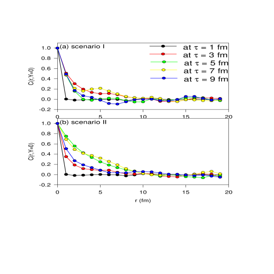
FIG. 1.: Evolution of the pion correlation fucntion with time, in scenario I and II.

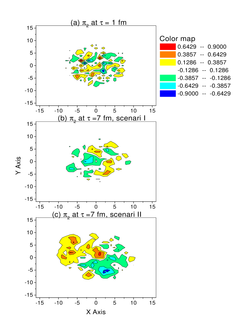
FIG. 2.: Contour plot of the $\pi_{2}$ component of the pion field at rapidity Y=0, at initial time $\tau_{i}$=1 fm/c and after evolution for 7 fm/c.

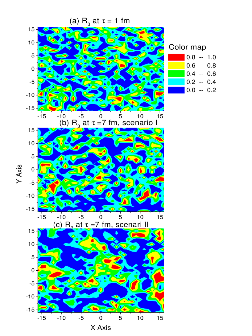
FIG. 3.: Contour plot of the neutral to total pion ratio, at rapidity Y=0, at initial time $\tau_{i}$=1 fm/c and after evolution for 7 fm/c.

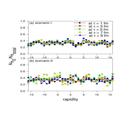
FIG. 4.: Rapidity distribution of neutral to total pion ratio, in scenario I and II. The ratio at different time intervals are shown.

REFERENCES

- [1] e-mail address:akc@veccal.ernet.in
- [2] K. Rajagopal and F. Wilczek, Nucl.Phys.B404,577,(1993). K. Rajagopal and F. Wilczek, Nucl.Phys.B399,395,(1993). K. Rajagopal, Nucl.Phys.A566,567c(1994).
- [3] J. D. Bjorken, K. L. Kowalski and C. C. Taylor , SLAC-PUB-6109 (1993), K.L. Kowalski K. L. and Taylor C. C., CWRUTH-92-6 (1992),hep-ph/9211282. J. D. Bjorken, Acta Phys. Polon. B28,2773 (1997).
- [4] A. A. Anselm and M. G. Ryskin , Phys. Lett. B 266,482 (1991), A. A. Aneslm, Phys. Lett. B217, 169(1988).
- [5] C. M. G. Lattes, Y. Fujimoto and S. Hasegawa, Phys. Reports, 154,247(1980).
- [6] J. Randrup, Phys. Rev D55,1188 (1997). J. Randrup, Nucl. Phys. A616,531 (1997). J. Randrup and R. L. Thews, Phys. Rev. D56,4392(1997). J. Schaffner-Bielich and Jorgen Randrup, Phys. Rev. C59,3329 (1999). J. Randrup, Heavy ion Phys. 9,289 (1999).
- [7] Gavin S., Gocksch A. and Pisarski R. D., Phys. Rev. Lett.72 2143, (1994). Gavin S. and Muller B. Phys. Lett.B329 486 (1994). S. Gavin, Nucl. Phys. A590,163c,1995
- [8] M. Asakawa, Z. Huang and X.N. Wang, Nucl. Phys. A590, 575c (1995). M. Asakawa, Z. Huang and X.N. Wang, hep-ph/9408299, Phys. Rev. Lett. 74 (1995) 3126. M. Asakawa, H. Minakata and B. Muller, Phys.Rev.D58, 094011(1998). M. Asakawa, H. Minakata and B. Muller, Nucl. Phys. A638,443c (1998).
- [9] A. Bochkarev and J. Kapusta, Phys. Rev. D54 4066 (1996).
- [10] C. Greiner and B. Müller, Phys. rev. D 55 1026 (1997).
- [11] T. S. Biro and C. Greiner, Phys. Rev. Lett. 79, 3138(1997).
- [12] Z. Zu and C. Greiner, hep-ph/9910562, Phys. Rev. D 62 036012 (2000).
- [13] D. H. Rischke, Phys. Rev. C, 2331 (1998)
- [14] A. K. Chaudhuri, nucl-th/9809018, Phys. Rev. D. 59 117503 (1999).
- [15] A. K. Chaudhuri, hep-ph/9904269
- [16] A. K. Chaudhuri, hep-ph/9908376
- [17] A. K. Chaudhuri, hep-ph/0007332