SLAC-PUB-8635 FERMILAB-PUB-00/286-T October 2000

Signals for Non-Commutative Interactions at
Linear Colliders

JoAnne L. Hewett^a,b, Frank J. Petriello^a, and Thomas G. Rizzo^{a a}Stanford Linear Accelerator Center

Stanford University

Stanford CA 94309, USA

^bFermi National Accelerator Laboratory

Batavia, IL 60510, USA

Recent theoretical results have demonstrated that non-commutative geometries naturally appear within the context of string/M-theory. One consequence of this possibility is that QED takes on a non-abelian nature due to the introduction of 3- and 4-point functions. In addition, each QED vertex acquires a momentum dependent phase factor. We parameterize the effects of non-commutative space-time co-ordinates and show that they lead to observable signatures in several $2\rightarrow 2$ QED processes in $e^{+}e^{-}$ collisions. In particular, we examine pair annihilation, Moller and Bhabha scattering, as well as $\gamma\gamma\rightarrow\gamma\gamma$ scattering and show that non-commutative scales of order a TeV can be probed at high energy linear colliders.

1 Introduction and Background

Although the full details of string/M-theory have yet to be unraveled, this theoretical effort has inspired a number of ideas over the years which have had significant impact on the phenomenology of particle physics. Two such examples are given by the string-inspired $E_{6}$ models of the late 1980’s[1] and the ongoing endeavor in building realistic and testable models from theories which have additional space-time dimensions[2]. Most recently, a resurgence of interest in non-commutative quantum field theory (NCQFT) and its applications[3] has developed within the context of string theory. Of course non-commutative theories are also interesting in their own right. However, it has yet to be explored whether they have any connection with the physics of the Standard Model (SM) or whether their effects could be observable in laboratory experiments. It is the purpose of this paper to begin to address these questions.

An exhaustive introduction to NCQFT is beyond the scope of the present treatment, hence we will simply outline some of the basics of the theory as well as some results which are relevant to the phenomenological analysis that follows. We will see that NCQFT results in modifications to QED which can be probed in $2\rightarrow 2$ processes in $e^{+}e^{-}$ collisions.

The essential idea of NCQFT is a generalization of the usual d-dimensional space, $R^{d}$, associated with commuting space-time coordinates to one which is non-commuting, $R^{d}_{\theta}$. In such a space the conventional coordinates are represented by operators which no longer commute, i.e.,

$$[\hat{X}_{\mu},\hat{X}_{\nu}]=i\theta_{\mu\nu}\equiv{i\over{\Lambda_{NC}^{2}}}c_{\mu\nu}\,.$$ (1)

In the last equality we have parameterized the effect in terms of an overall scale $\Lambda_{NC}$, which characterizes the threshold where non-commutative (NC) effects become relevant, and a real antisymmetric matrix $c_{\mu\nu}$, whose dimensionless elements are presumably of order unity. From our point of view the role of the NC scale $\Lambda_{NC}$ can be compared to that of $\hbar$ in conventional Quantum Mechanics which represents the level of non-commutativity between coordinates and momenta. A priori the scale $\Lambda_{NC}$ can take any value, perhaps the most likely being of order the Planck scale $\overline{M}_{Pl}$. However, given the possibility[2] of the onset of stringy effects at the TeV scale, and that values of the scale where gravity becomes strong in models with large extra dimensions can be of order a TeV, it is feasible that NC effects could also set in at a TeV. Here, we adopt this spirit and consider the possibility that $\Lambda_{NC}$ may not lie far above the TeV scale.

Note that the matrix $c_{\mu\nu}$ is not a tensor since its elements are identical in all reference frames. This leads immediately to a violation of Lorentz invariance which is quite different than that discussed most often in the literature[4] since it sets in only at energies of order $\Lambda_{NC}$. As we will see below, this violation will take the form of dimension-8 operators for the processes we consider and is thus highly suppressed at low energies. In addition, there exists a more than superficial relation between the anti-symmetric matrix $c_{\mu\nu}$ and the Maxwell field strength tensor $F_{\mu\nu}$ as NCQFT arises in string theory[5] through the quantization of strings, described by the low energy excitations of D-branes in the presence of background electromagnetic fields. The space-time components, $c_{0i}$, thus define the direction of a background E field, while the space-space components, $c_{ij}$, describe the direction of a background magnetic or string B field. Geometrically, we can then think of $c_{0i}$ and $c_{ij}$ as two 3-vectors that point in a specific pair of preferred directions in the laboratory frame. Theories with $c_{0i}(c_{ij})\neq 0$ are usually referred to as space-time(space-space) non-commutative.

NCQFT can be phrased in terms of conventional commuting QFT through the application of the Weyl-Moyal correspondence[6]

$$\hat{A}(\hat{X})\longleftrightarrow A(x)\,,$$ (2)

where $A$ represents a quantum field with $\hat{X}$ being the set of non-commuting coordinates and $x$ corresponding to the commuting set. However, in formulating NCQFT, one must be careful to preserve orderings in expressions such as $\hat{A}(\hat{X})\hat{B}(\hat{X})$. This is accomplished with the introduction of a star product, $\hat{A}(\hat{X})\hat{B}(\hat{X})=A(x)*B(x)$, where the effect of the commutation relation is absorbed into the star. Making the Fourier transform pair

$$\hat{A}(\hat{X}) = {1\over{(2\pi)^{d/2}}}\int~{}d\alpha e^{i\alpha\hat{X}}~{}a(\alpha)$$

$$a(\alpha) = {1\over{(2\pi)^{d/2}}}\int~{}dxe^{-i\alpha x}~{}A(x)\,,$$ (3)

with $x$ and $\alpha$ being real n-dimensional variables, allows us to write the product of two fields as

$$\hat{A}(\hat{X})\hat{B}(\hat{X}) = {1\over{(2\pi)^{d}}}\int~{}d\alpha d\beta e^{i\alpha\hat{X}}~{}a(\alpha)e^{i\beta\hat{X}}~{}b(\beta)$$ (4)

$$= {1\over{(2\pi)^{d}}}\int~{}d\alpha d\beta~{}e^{i(\alpha+\beta)\hat{X}-{1\over{2}}\alpha^{\mu}\beta^{\nu}[\hat{X}_{\mu},\hat{X}_{\nu}]}a(\alpha)b(\beta)\,.$$

We thus have the correspondence

$$\hat{A}(\hat{X})\hat{B}(\hat{X})\longleftrightarrow A(x)*B(x)\,,$$ (5)

provided we identify

$$A(x)*B(x)\equiv\bigg{[}e^{{i\over{2}}\theta_{\mu\nu}\partial_{\zeta\mu}\partial_{\eta\nu}}A(x+\zeta)B(z+\eta)\bigg{]}_{\zeta=\eta=0}\,.$$ (6)

Note that to leading order in $\theta$ the $*$ product is given by

$$A(x)*B(x)=AB+{i\over{2}}\theta^{\mu\nu}\partial_{\mu}A\partial_{\nu}B+{\cal O}(\theta^{2})\,.$$ (7)

Hence the non-commutative version of an action for a quantum field theory can be obtained from the ordinary one by replacing the products of fields by star products. In doing so it is useful to define a generalized commutator, known as the Moyal bracket, for two quantities $S,T$ as

$$[S,T]_{MB}=S*T-T*S\,,$$ (8)

so that the Moyal bracket of any quantity with itself vanishes. Note that the integration of a Moyal bracket of two quantities over all space-time vanishes, i.e.,

$$\int~{}d^{4}x~{}[S(x),T(x)]_{MB}=0\,,$$ (9)

which means they commute inside the integral. This can be generalized to show that the integral of a $*$ product of an arbitrary number of quantities is invariant under cyclic permutations in a manner similar to the trace of ordinary matrices. We also note that the Moyal bracket of two coordinates

$$[x_{\mu},x_{\nu}]_{MB}=x_{\mu}*x_{\nu}-x_{\nu}*x_{\mu}\,,$$ (10)

mimics the operator commutation relation in Eq. (1).

Once the products of fields are replaced by $*$ products, infinite numbers of derivatives of fields can now appear in an action, implying that all such theories are non-local. This is not surprising since, in analogy with ordinary Quantum Mechanics, one now has a spacetime uncertainty relation

$$\Delta\hat{X}^{\mu}\Delta\hat{X}^{\nu}\geq{1\over{2}}|\theta^{\mu\nu}|\,.$$ (11)

Theories with $c_{0i}\neq 0$ have an additional problematic feature in that they generally do not have a unitary $S$-matrix[7], at least in perturbation theory, since an infinite number of time derivatives are involved in $*$ products. However, it has recently been shown[8] that it may be possible to unitarize the space-time case by combining the spacial NC Super Yang Mills limit with a Lorentz transformation with finite boost velocity. On the other hand, theories with only space-space non-commutativity, $c_{ij}\neq 0$, are unitary.

There are a number of important results in NCQFT which we now state without proof, referring the interested reader to the original papers for detailed explanations. ($i$) Matsubara[9] has shown that only the $U(n)$ matrix Lie algebra is closed under the Moyal bracket, thus non-commutative gauge theories can be constructed only if they are based upon these gauge groups. Hence in order to embed the full SM in NCQFT, the usual Standard Model $SU(n)$ group factors must be extended to $U(n)$ groups. However, due to the effective non-abelian nature of the Moyal brackets, these $U(n)$ groups cannot be simply decomposed into products of $SU(n)$ and $U(1)$ factors. ($ii$) There are indications that conventional renormalizable, gauge invariant field theories remain renormalizable and gauge invariant when generalized to non-commutative spacetimes[10], although a proof does not yet exist for theories which are spontaneously broken[11]. ($iii$) Non-commutative QED, based on the group $U(1)$, has been studied by several groups[12, 13]; due to the presence of $*$ products and Moyal brackets, the theory takes on a non-abelian nature in that both 3-point and 4-point photon couplings are generated. The photonic part of the action is now

$$S_{NCQED}={-1\over{4}}\int~{}d^{4}x~{}F_{\mu\nu}*F^{\mu\nu}={-1\over{4}}\int~{}d^{4}x~{}F_{\mu\nu}F^{\mu\nu}\,,$$ (12)

where the second equality follows from the commutativity of Moyal brackets under integration, shown in Eq. (9). This action is gauge invariant under a local transformation $U(x)$ with $F_{\mu\nu}$ defined as

$$F_{\mu\nu}=\partial_{\mu}A_{\nu}-\partial_{\nu}A_{\mu}-i[A_{\mu},A_{\nu}]_{MB}\,.$$ (13)

The origin of the 3- and 4-point functions is now readily transparent. Note that the photon’s 2-point function is identical in commutative and NC spaces because quadratic forms remain unchanged. When performing the Fourier transformation of these new interactions into momentum space, the vertices pick up additional phase factors which are dependent upon the momenta flowing through the vertices. We will see below that these kinematic phases will play an important role in the collider tests of NCQFT. ($iv$) When fermions are added to the theory, covariant derivatives can only be constructed for fields of charge $0,\pm 1$. The structure of those derivatives for the $Q=\pm 1$ case is similar to that for fundamental and anti-fundamental representations in non-abelian theories. The covariant derivatives for neutral fields are either trivial (as in the case of abelian commutative $U(1)$ theory) or correspond to what would ordinarily be called the adjoint representation in the case of a commutative non-abelian theory. As before, the three-point function picks up an additional kinematic phase from the Fourier transformation of the interaction term into momentum space. This is shown explicitly in Fig. 1. The general form of the Feynman rules for NCQED can be found in Ref.[14]; the ones of relevance to the processes considered in this paper are displayed in Fig. 1. ($v$) NCQED with fermions and space-space non-commutativity has been shown[15] to be CP violating yet CPT conserving.

Figure 1: Feynman rules of NCQED.

Having now presented the basic formalism of NCQFT and subsequent modifications to QED, in the following sections we examine the effects in several $2\rightarrow 2$ processes in $e^{+}e^{-}$ collisions, including pair annihilation, Moller and Bhabha scattering, as well as in $\gamma\gamma\rightarrow\gamma\gamma$ scattering. We will see that the lowest order correction to the SM results for these transitions is given by dimension-8 operators. In addition, we find that an oscillatory azimuthal dependence is induced in these processes due to the preferred direction in the laboratory frame defined by the NC matrix $c_{\mu\nu}$. In summary, we will see that high energy linear colliders can probe non-commutative scales of order a TeV.

Before discussing our analysis for the specific processes considered here, a few additional comments are in order regarding the observation of these non-commutative effects. First, as discussed above, the vectors $c^{E}_{i}=[c_{0i}]$ and $c^{B}_{i}=[\epsilon_{ijk}c_{jk}]$ point in fixed specific directions which are the same in all reference frames. In our analysis below we define the $z$-axis as that corresponding to the direction of the incoming particles in a fixed laboratory frame with the vectors c having arbitrary components in that frame. Now, imagine a second laboratory at a different point on the surface of the Earth performing the same experiment. Clearly the co-ordinate systems of the two laboratories will be different, i.e., the beam directions and hence the $z$-axis will not be the same in the two locations. This implies that the experimentally determined values for the components of the c vectors will differ at the two laboratory sites due to their locally chosen set of co-ordinates. Hence both laboratories must convert their local co-ordinates to a common frame, e.g., with respect to the rest frame of the 3 degree K blackbody radiation or some other slowly varying astronomical co-ordinate system, so that they would measure equivalent directions and magnitudes for c. This translation of co-ordinates to a common frame will be necessary if we are to compare the results of multiple experiments for signals of non-commutativity.

In addition, even for a single experiment, the apparent directions of the c vectors will vary with time due to the rotation of the Earth and its revolution about the Sun. While the actual c vectors will always point to the same position on the sky, the co-ordinates of this position will vary continuously in the laboratory frame due to the Earth’s motion. (The effects of galactic motion should be small during the life-span of any given experiment.) Collider experiments will thus have to make use of astronometric techniques to continuously translate their laboratory co-ordinates to astronomical ones such that when events are recorded the relative orientation of the two frames would be accounted for. This should be a rather straightforward procedure for any future collider experiment to implement given that many non-accelerator based experiments already make use of these ideas.

Taking the Earth’s motion into account is particularly important for experiments which measure observable quantities that are odd in c, including for example, the $g-2$ of the muon[12], the Lamb shift[16], as well as other processes which are linear[17] in the NC parameter. If only the laboratory co-ordinates were employed, at least some of the components of c would average to zero over a sidereal day. In the cases we discuss below, the observables are even functions of c, and while we would not obtain a null effect, time averaging would result in a diminished sensitivity to $\Lambda_{NC}$.

2 Moller Scattering

For all of the scattering processes considered in this paper, except for $\gamma\gamma\rightarrow\gamma\gamma$, we can define the momenta of the incoming, represented by $p_{1,2}$, and outgoing, corresponding to $k_{1,2}$, particles in terms of the coordinates fixed in the laboratory as

$$\begin{array}[]{rcl}p_{1}^{\mu}&=&{{\sqrt{s}}\over{2}}(1,-1,0,0)\\ k_{1}^{\mu}&=&{{\sqrt{s}}\over{2}}(1,-c_{\theta},-s_{\theta}c_{\phi},-s_{\theta}s_{\phi})\end{array}\qquad\begin{array}[]{rcl}p_{2}^{\mu}&=&{{\sqrt{s}}\over{2}}(1,1,0,0)\\ k_{2}^{\mu}&=&{{\sqrt{s}}\over{2}}(1,c_{\theta},s_{\theta}c_{\phi},s_{\theta}s_{\phi})\,.\end{array}$$ (14)

Note that the ordering of the co-ordinates used in these definitions is given by $(t,z,x,y)$, so that the $z$-axis is along the beam direction as usual. Using these definitions, the bilinear products of these momenta with the matrix $c_{\mu\nu}$, which appear in the Feynman rules of Fig. 1, can be calculated to be

$$p_{1}\cdot c\cdot p_{2} = {s\over{2}}c_{01}$$

$$k_{1}\cdot c\cdot k_{2} = {s\over{2}}[c_{01}c_{\theta}+c_{02}s_{\theta}c_{\phi}+c_{03}s_{\theta}s_{\phi}]$$

$$p_{1}\cdot c\cdot k_{1} = {s\over{4}}[c_{01}(1-c_{\theta})+(c_{12}-c_{02})s_{\theta}c_{\phi}-(c_{03}+c_{31})s_{\theta}s_{\phi}]$$

$$p_{1}\cdot c\cdot k_{2} = {s\over{4}}[c_{01}(1+c_{\theta})-(c_{12}-c_{02})s_{\theta}c_{\phi}+(c_{03}+c_{31})s_{\theta}s_{\phi}]$$

$$p_{2}\cdot c\cdot k_{1} = {s\over{4}}[-c_{01}(1+c_{\theta})-(c_{12}+c_{02})s_{\theta}c_{\phi}-(c_{03}-c_{31})s_{\theta}s_{\phi}]$$ (15)

$$p_{2}\cdot c\cdot k_{2} = {s\over{4}}[-c_{01}(1-c_{\theta})+(c_{12}+c_{02})s_{\theta}c_{\phi}+(c_{03}-c_{31})s_{\theta}s_{\phi}]\,.$$

We remind the reader of the fact that $a\cdot c\cdot a=0$ for all vectors $a$ due to the antisymmetry of the matrix $c$. Note that $c_{23}$ does not appear in any of the above expressions since we have defined the $z$-axis to be along the direction of the initial beams and there is no B field associated non-commutative asymmetry relative to this direction.

The Feynman diagrams which mediate Moller scattering are displayed in Fig. 2. In this case, the NC modifications correspond to the kinematic phase which appears in each vertex. The question here is how to treat the $Z$-boson exchange contribution. While NCQED is a well defined theory, it is not immediately clear how to extend it to the full SM in a naive way even if we are only interested in tree-level fermionic interactions. Without such guidelines we see that there exist three possibilities: (i) the simplest case is if the $Z$ and photon have the same vertex structure as shown in Fig. 1, (ii) the full theory and appropriate $Zf\bar{f}$ kinematic phase are more complex, or (iii) only $\gamma f\bar{f}$ vertices pick up kinematic phases. Clearly, as far as signatures of non-commutativity are concerned, cases one and three will be qualitatively similar. Hence, for simplicity, we assume that the first possibility is realized.

Figure 2: Feynman graphs contributing to Moller scattering with the exchanged particle corresponding to a photon and $Z$-boson.

Following the Feynman rules of Fig. 1 and the momentum labeling given in Fig. 2 we see that the $t$- and $u$-channel exchange graphs now pick up kinematic phases given by

$$\phi_{t} = {1\over{2}}[p_{1}\cdot\theta\cdot k_{1}+p_{2}\cdot\theta\cdot k_{2}]$$

$$\phi_{u} = {1\over{2}}[p_{1}\cdot\theta\cdot k_{2}+p_{2}\cdot\theta\cdot k_{1}]\,.$$ (16)

Clearly, only the interference terms between the $t$- and $u$-channel diagrams pick up a relative phase when the full amplitude is squared. We define this phase as $\Delta_{Moller}$ and find it to be given by

$$\Delta_{Moller}=\phi_{u}-\phi_{t}={-{\sqrt{ut}}\over{\Lambda_{NC}^{2}}}[c_{12}c_{\phi}-c_{31}s_{\phi}]\,,$$ (17)

with the second equality following from Eq. (15). (We define the Mandelstam variables as usual: $t,u=-s(1\mp\cos\theta)/2$.) Hence the resulting differential distributions for this process appear exactly as in the SM except that the $t,u$-channel interference terms should be multiplied by $\cos\Delta_{Moller}$. Note that all of the terms involving time-space non-commutativity have dropped out of the expression for $\Delta_{Moller}$. In addition, as we take the limit $\Lambda_{NC}\rightarrow\infty$, $\cos\Delta\rightarrow 1$ so that the SM is recovered. In the limit of small $s/\Lambda^{2}_{NC}$, $\cos\Delta_{Moller}$ can be expanded where it is seen that the lowest order correction to the SM occurs at dimension-8. This is similar to the case of graviton exchange[18] in models with large extra dimensions[19] or in the Randall-Sundrum model of localized gravity[20] below threshold for graviton resonance production[21]. Perhaps the most important thing to notice, as discussed above, is that $\Delta_{Moller}\neq 0$ induces a $\phi$ dependence in a $2\rightarrow 2$ scattering process since there now exists a preferred direction in the laboratory frame.

For simplicity in our numerical results presented below, we will only consider the case $c_{12}\neq 0$. If instead $c_{31}$ is non-zero, the results will be similar except for the phase of the $\phi$ dependence. When both terms are present, the situation is in general somewhat more complex, yet will be qualitatively comparable to the case analysed below. Since we only consider one non-vanishing value of $c_{ij}$ at a time, we set its magnitude to unity when obtaining our results.

The differential cross section for Moller scattering in the laboratory center of mass frame can be written as

$${d\sigma\over{dz~{}d\phi}}={\alpha^{2}\over{4s}}\bigg{[}(e_{ij}+f_{ij})\big{(}P^{uu}_{ij}+P^{tt}_{ij}+2P^{ut}_{ij}\cos\Delta_{Moller}\big{)}+(e_{ij}-f_{ij})\big{(}{t^{2}\over{s^{2}}}P^{uu}_{ij}+{u^{2}\over{s^{2}}}P^{tt}_{ij}\big{)}\bigg{]}\,,$$ (18)

where $z=\cos\theta$, a sum over the gauge boson indices is implied, $e_{ij}=(v_{i}v_{j}+a_{i}a_{j})^{2}$ and $f_{ij}=(v_{i}a_{j}+a_{i}v_{j})^{2}$ are combinations of the electron’s vector and axial vector couplings and

$$P^{qr}_{ij}=s^{2}{{(q-m_{i}^{2})(r-m_{j}^{2})+\Gamma_{i}\Gamma_{j}m_{i}m_{j}}\over{[(q-m_{i}^{2})^{2}+(\Gamma_{i}m_{i})^{2}][(r-m_{j}^{2})^{2}+(\Gamma_{j}m_{j})^{2}]}}\,,$$ (19)

with $m_{i}(\Gamma_{i})$ being the mass (width) of the $i^{th}$ gauge boson, where $i$=1(2) corresponds to the photon($Z$). The expression for the differential Left-Right Polarization asymmetry, $A_{LR}(z,\phi)$, can be easily obtained from the above by forming the ratio

$$A_{LR}(z,\phi)=N(z,\phi)/D(z,\phi)\,,$$ (20)

where $D(z,\phi)$ is the differential cross section expression above and $N(z,\phi)$ can be obtained from $D(z,\phi)$ by the redefinition of the coupling combinations $e_{ij}$ and $f_{ij}$ as

$$e_{ij}=f_{ij}=(v_{i}v_{j}+a_{i}a_{j})(v_{i}a_{j}+a_{i}v_{j})\,.$$ (21)

Although we have expressed the cross section in an apparently covariant form using Mandelstam variables, it is not actually invariant due to the presence of $\Delta_{Moller}$ which is highly frame dependent.

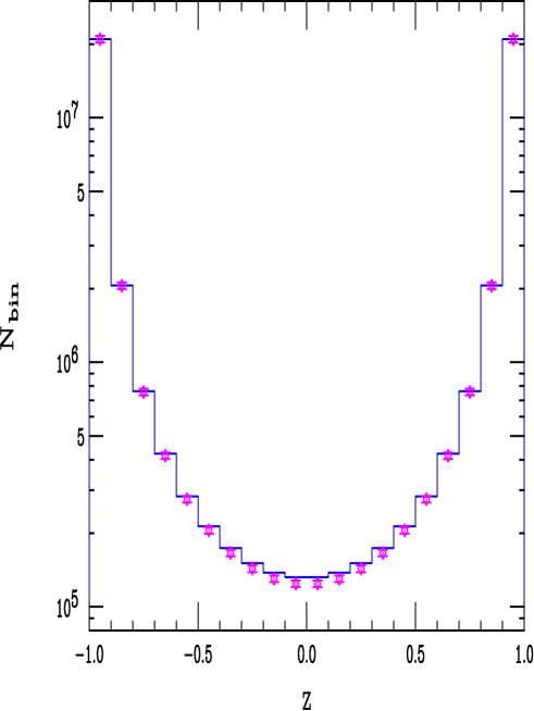
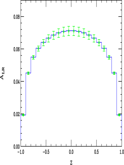
Figure 3: Binned cross section (top) and polarized asymmetry (bottom) as a function of $z=\cos\theta$ for Moller scattering at a 500 GeV linear collider assuming an integrated luminosity of 300 fb^-1. The histogram is the SM expectation while the data corresponds to $\Lambda_{NC}=\sqrt{s}$.

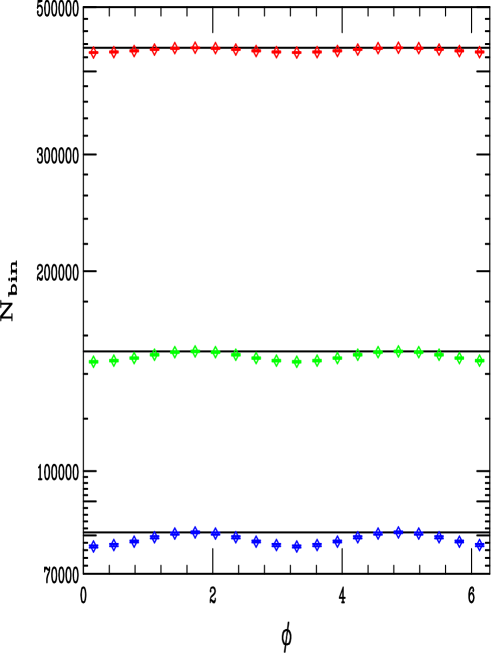
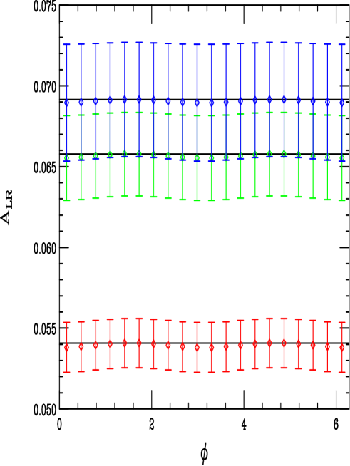
Figure 4: $\phi$ dependence of the Moller cross section (top) and left-right asymmetry (bottom) for the SM (straight lines) and for the case $\Lambda_{NC}=\sqrt{s}$ (shown as data) at a 500 GeV linear collider with a luminosity of 300 fb^-1. From top to bottom in the top panel a $z$ cut of 0.9(0.7, 0.5) has been applied with the order reversed in the lower panel.

Figure 3 displays the effect of a finite value of $\Lambda_{NC}=\sqrt{s}$ on the shape of the conventional bin-integrated, $z$-dependent event rate and $A_{LR}$ for a 500 GeV linear collider assuming an integrated luminosity of 300 $fb^{-1}$. In presenting these results we have neglected initial state radiation and beamstrahlung effects, assumed both beams are $90\%$ polarized with $\delta P/P=0.003$, and taken an overall luminosity error of $1\%$. Angular cuts of $\theta=10^{o}$ have also been applied but the entire $\phi$ range has been integrated over. As we can see from this figure, the influence of $\Lambda_{NC}^{-1}\neq 0$ appears to cause a small downward shift in the $\cos\theta$ distribution which is most noticeable at large scattering angles away from the forward and backward $t$- and $u$-channel poles from the photon exchange graph. The effect of a finite value of $\Delta_{Moller}$ is thus seen to increase the amount of destructive interference between the $u$- and $t$-channel graphs. Although the shift is apparently small it occurs over many bins and is statistically quite significant given the size of the errors at this integrated luminosity. For $A_{LR}$ there is hardly any shift from the SM values in this case.

Figure 4 presents the $z$-integrated, $\phi$ dependent distribution for both the rate and $A_{LR}$. Note that as we perform more restrictive cuts on $|z|$, the central region, which is the most sensitive to $\Lambda_{NC}$, is becoming more isolated. As can be seen from the figures, this approach enhances the $\phi$ dependence for the differential cross section. Though the $\phi$ dependence also appears to be rather weak, it is again statistically significant at this large integrated luminosity. As in the case of the $\phi$-integrated $A_{LR}$, the $z$-integrated $A_{LR}$ shows hardly any sensitivity to finite $\Lambda_{NC}$ even when a strong $|z|$ cut is applied.

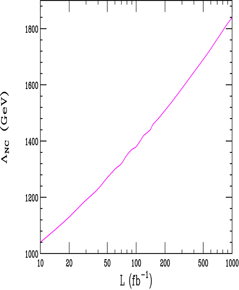
Figure 5: $95\%$ CL lower bound on $\Lambda_{NC}$ at a 500 GeV linear collider as a function of the integrated luminosity from Moller scattering via the fit described in the text.

In order to obtain a $95\%$ CL lower bound on $\Lambda_{NC}$ from Moller scattering we perform a combined fit to the total cross section, the shape of the doubly differential $z-\phi$ angular distribution and $A_{LR}(z,\phi)$. In the latter two cases we bin the NC results in a $20\times 20$ array of $z,\phi$ values and employ only statistical errors apart from the polarization uncertainty. In the case of the total rate we also include the luminosity uncertainty in the error. For a fixed value of luminosity we then compare the predictions of the SM with the case where $\Lambda_{NC}$ is finite and repeat this procedure by varying $\Lambda_{NC}$ until we obtain a $95\%$ CL bound by using a $\chi^{2}$ fit. From this procedure we obtain the search reach on $\Lambda_{NC}$ as a function of the integrated luminosity as displayed in Fig. 5. As we can see from this figure, bounds on $\Lambda_{NC}$ of order $(3-3.5)\sqrt{s}$ are obtained for reasonable luminosities.

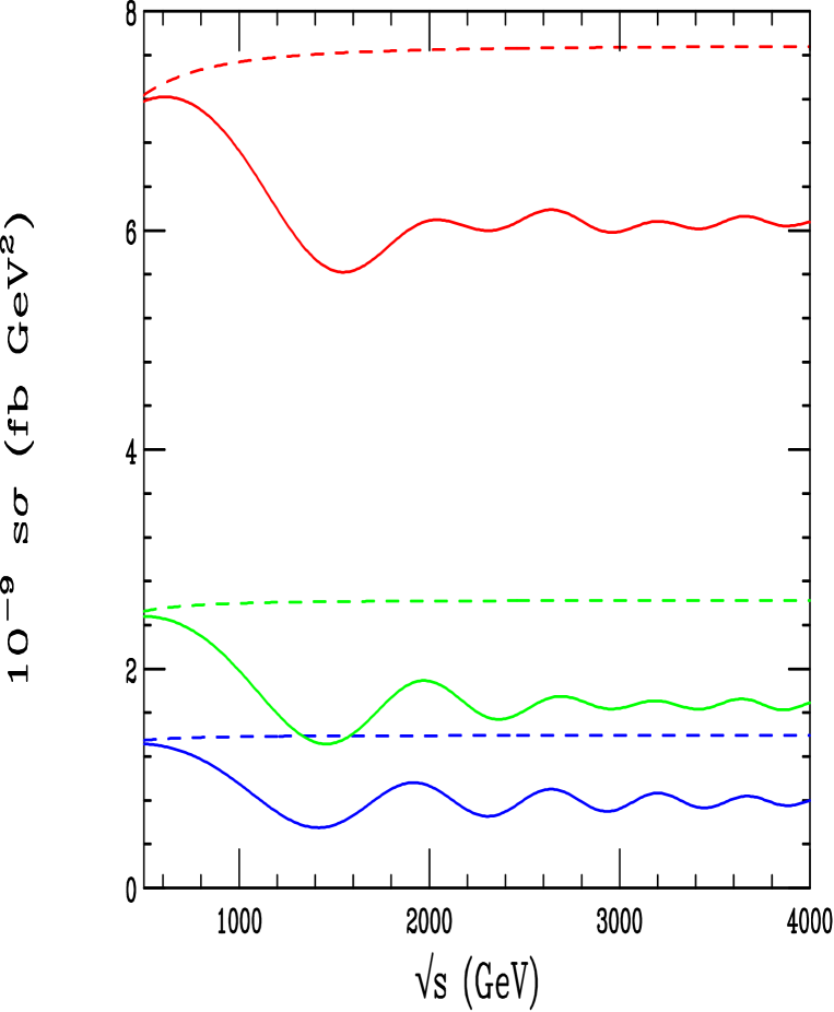
Figure 6: Scaled dependence of the Moller total cross section, subject to a angular cut (from top to bottom) of $|z|\leq 0.9(0.7,~{}0.5)$ assuming the SM (dashed curves) or $\Lambda_{NC}=$500 GeV (solid curves).

We now examine how the Moller cross section behaves as $\sqrt{s}$ grows beyond $\Lambda_{NC}$. In the SM for large $s$ we expect the scaled cross section, i.e., the product $s\cdot\sigma_{Moll}$, to be roughly constant after a cut on $|\cos\theta|$ cut is performed. Ordinarily when new operators are introduced, the modified scaled cross section is expected to grow rapidly near the appropriate scale beyond which the contact interaction limit no longer applies. However, in the present case, the theory above the scale $\Lambda_{NC}$ is a well-defined theory since it is not a low energy limit. We would thus anticipate that the $\cos\Delta_{Moller}$ factor leads to a modulation of the scaled cross section that averages out rapidly with a period that depends on the hardness of the $|\cos\theta|$ cut as the value of $\sqrt{s}$ increases. This effect is displayed in Fig. 6 and behaves exactly as expected.

3 Bhabha Scattering

The Feynman graphs which mediate Bhabha scattering in NCQED are given in Fig. 7. In this case, the $t$-and $s$-channel kinematic phases are now given by

$$\phi_{t} = {-1\over{2}}[p_{1}\cdot\theta\cdot k_{1}-p_{2}\cdot\theta\cdot k_{2}]$$

$$\phi_{s} = {-1\over{2}}[p_{1}\cdot\theta\cdot p_{2}-k_{1}\cdot\theta\cdot k_{2}]\,,$$ (22)

which implies that the interference term between the two amplitudes is sensitive to $\cos\Delta_{Bhabha}$ which is given by

$$\Delta_{Bhabha}=\phi_{s}-\phi_{t}={-1\over{\Lambda_{NC}^{2}}}[c_{01}t+{\sqrt{ut}}(c_{02}c_{\phi}+c_{03}s_{\phi})]\,.$$ (23)

Note that whereas Moller scattering was sensitive to space-space non-commutativity we see that Bhabha scattering is instead sensitive to time-space non-commutativity. Here we see that there are two distinct cases depending whether or not $\Delta_{Bhabha}$ has a $\phi$ dependence. If $c_{01}$ is non-zero then the $\phi$ dependence will be absent, whereas the two cases $c_{02},c_{03}\neq 0$ are essentially identical except for the phase of the $\phi$ dependence. We thus only consider the cases $c_{01}=1$ or $c_{02}=1$.

Figure 7: Feynman graphs contributing to Bhabha scattering with the exchanged particle corresponding to a photon and $Z$-boson.

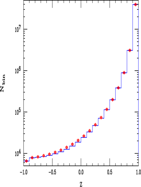
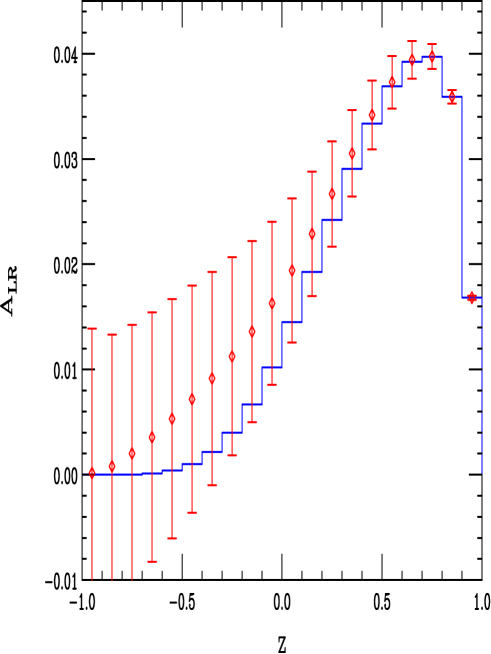
Figure 8: Same as Fig. 3 but now for Bhabha scattering assuming that $c_{01}$ is non-zero.

Using the notation above, the differential cross section in the laboratory center of mass frame for Bhabha scattering can then be written as

$${d\sigma\over{dz~{}d\phi}}={\alpha^{2}\over{2s}}\bigg{[}(e_{ij}+f_{ij})\big{(}P^{ss}_{ij}+P^{tt}_{ij}+2P^{st}_{ij}\cos\Delta_{Bhabha}\big{)}{u^{2}\over{s^{2}}}+(e_{ij}-f_{ij})\big{(}P^{ss}_{ij}{t^{2}\over{s^{2}}}+P^{tt}_{ij}\big{)}\bigg{]}\,,$$ (24)

with $A_{LR}(z,\phi)$ defined in a manner similar to that for Moller scattering by forming the ratio $N(z,\phi)/D(z,\phi)$.

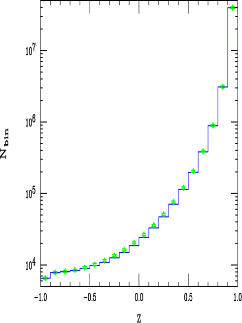
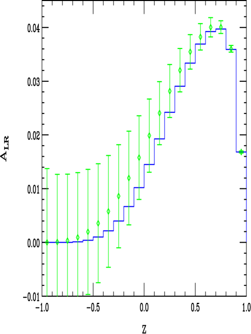
Figure 9: Same as in Fig. 8 but now assuming that $c_{02}$ is non-zero.

We first consider the case where $c_{01}$ is taken to be non-zero. Figure 8 displays the (in this case trivial) $\phi$ integrated angular distribution and $A_{LR}$ for the SM with $\Lambda_{NC}=\sqrt{s}=500$ GeV. Here one sees that a finite value of $\Lambda_{NC}^{-1}$ leads to a slight increase in the cross section at large angles and a moderate change in $A_{LR}$ in the same $z$ range. In the case where $c_{02}$ is non-zero, Fig. 9 shows the corresponding distributions. Note that the shift in the cross section looks almost identical in the two cases but the deviation in $A_{LR}$ is more shallow in the latter case. Figure 10 shows the $\phi$ dependence of the $z$-integrated distributions for the same three cuts on $\cos\theta$ discussed above in the case of Moller scattering. As before we see that the effect in the cross section is most visible for stiffer cuts which isolate the central region. In the case of $A_{LR}$ the $\phi$ dependence is too small at these integrated luminosities to be visible. In order to obtain a $95\%$ CL lower bound on $\Lambda_{NC}$ from Bhabha scattering we follow the same procedure as that discussed above for Moller scattering and obtain the results presented in Fig. 11. Here we see that the reach for $\Lambda_{NC}$ via Bhabha scattering is not quite as good as what we had found earlier for the case of Moller scattering, given only by $\simeq 2\sqrt{s}$, for both of the cases considered.

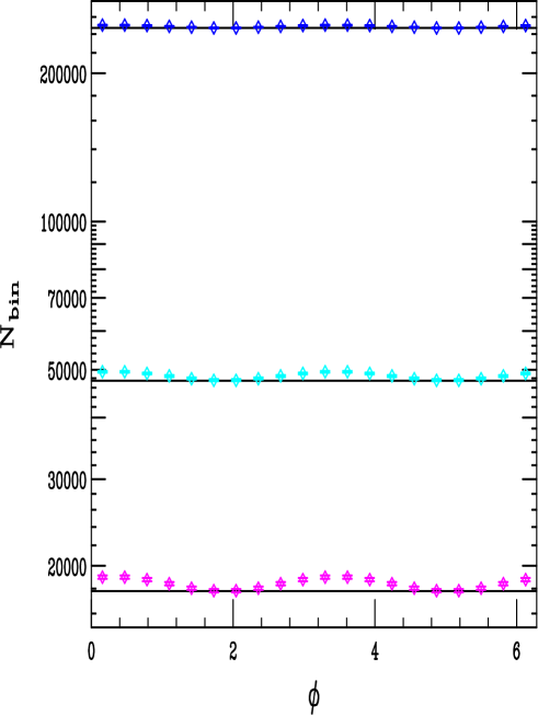
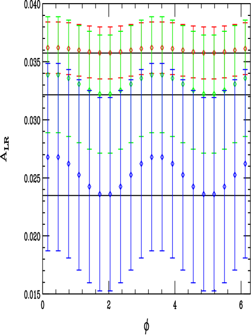
Figure 10: Same as Fig. 4 but now for Bhabha scattering with $c_{02}$ taken to be non-zero. The order for the cuts on $|\cos\theta|$ is reversed in the lower plot.

Figures 12 and 13 show the scaled cross sections for Bhabha scattering after the $z$ cuts are employed for values of $\sqrt{s}>\Lambda_{NC}$. Here we see that for both cases, the presence of a finite value for $\Delta_{Bhabha}$ leads to an increase in the constructive interference between the $s$- and $t$-channel exchanges with two very different periods. Again for values of $\sqrt{s}$ much larger than $\Lambda_{NC}$ we see that the oscillations average out to approximately half of their original amplitude.

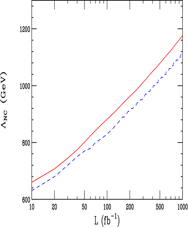
Figure 11: $95\%$ CL bounds on $\Lambda_{NC}$ as a function of luminosity from Bhabha scattering assuming either $c_{01}$ (solid) or $c_{02}$ (dashed) is non-zero.

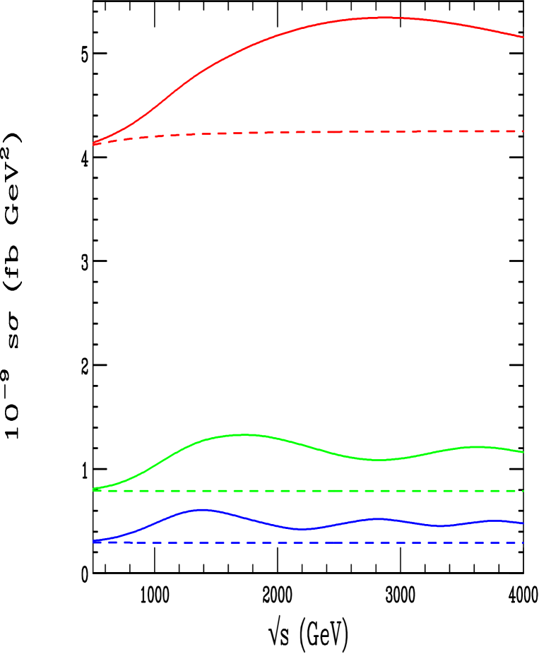
Figure 12: The scaled cross section for Bhabha scattering with $c_{01}$ non-zero.

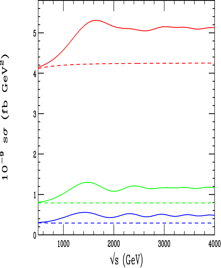
Figure 13: Same as in the previous figure but now with $c_{02}$ non-zero.

4 Pair Annihilation

The Feynman diagrams which contribute to pair annihilation in NCQED are shown in Fig. 14. Note that in this case, there is a novel s-channel contribution in NC field theories from the $3\gamma$ self-coupling, in addition to the kinematical phase factor which appears at each vertex. Due to the presence of the non-abelian like coupling, one must exercise caution in calculating the cross section to ensure that the Ward identities are satisfied and to guarantee that unphysical polarization states are not produced. Hence one must either extend the polarization sum to incorporate transverse photon polarization states or include the contribution from the production of a ghost-antighost pair to cancel the contribution of the unphysical gauge boson polarizations. This procedure is similar in manner to that performed for the parton-level scattering of $q\bar{q}\rightarrow gg$ in QCD. We find that the differential cross section in the laboratory center of mass frame for pair annihilation in NCQED is then given by

$$\frac{d\sigma}{dz\,d\phi}=\frac{\alpha^{2}}{4s}\,\bigg{[}\frac{u}{t}+\frac{t}{u}-4\,\frac{t^{2}+u^{2}}{s^{2}}\,{\rm sin}^{2}(\frac{1}{2}k_{1}\wedge k_{2})\bigg{]}\,,$$ (25)

where we have introduced the wedge product defined as $p\wedge k=p_{\mu}k_{\nu}\theta^{\mu\nu}$. Note that in this case, the contribution from the relative phases from the interference terms cancels. We also note that the sign of the modification due to NCQED does not vary since it is an even function and hence the effect does not wash out over time due to the rotation of the Earth.

Figure 14: The three tree level contributions to $e^{+}e^{-}\rightarrow\gamma\gamma$ in NCQED.

Evaluating the wedge product yields

$$\Delta_{PA}\equiv{1\over 2}k_{1}\wedge k_{2}=\frac{-s}{2\Lambda^{2}_{NC}}\bigg{[}c_{01}c_{\theta}+c_{02}s_{\theta}c_{\phi}+c_{03}s_{\theta}s_{\phi}\bigg{]}\,.$$ (26)

Note that this process is sensitive only to space-time non-commutativity. We again stress that this is only true in the CM frame; due to the violation of Lorentz invariance this will not hold in all reference frames. As discussed above, it is important to remember that although we have expressed the cross section in terms of the Lorentz invariant Mandelstam variables, $s\,,t\,,u$, the phase $\Delta_{PA}$ is not Lorentz invariant. For this reaction, we parameterize the $c_{0i}$ by introducing the angles characterizing the background E field of the theory:

$$c_{01} = {\rm cos}\alpha$$

$$c_{02} = {\rm sin}\alpha\,{\rm cos}\beta$$ (27)

$$c_{03} = {\rm sin}\alpha\,{\rm sin}\beta\,,$$

so that

$$\Delta_{PA} = \frac{-s}{2\Lambda^{2}_{NC}}\bigg{[}{\rm cos}\theta\,{\rm cos}\alpha+{\rm sin}\theta\,{\rm sin}\alpha\,{\rm cos}(\phi-\beta)\bigg{]}$$ (28)

$$= \frac{-s}{2\Lambda^{2}_{NC}}\,{\rm cos}\theta_{NC}\,,$$

where $\theta_{NC}$ is the angle between the E field and the direction of the outgoing photon denoted with momenta $k_{1}$. Note that $\beta$ simply defines the origin of the $\phi$ axis; we will hereafter set $\beta=\pi/2$. This parameterization provides a good physical interpretation of the NC effects. (Note that the $c_{0i}$ are not independent; in pulling out the overall scale $\Lambda_{NC}$ we can always impose the constraint $|c_{01}|^{2}+|c_{02}|^{2}+|c_{03}|^{2}=1$.) Here, we consider three physical cases: $\alpha=0$, $\alpha=\pi/2$, and $\alpha=\pi/4$, which correspond to the background E fields being at an angle $\alpha$ from the beam axis. The correction term $\Delta_{PA}$ then takes the following forms in each of these cases:

$$\Delta_{PA}(\alpha=0) = \frac{-s}{2\Lambda^{2}_{NC}}\,{\rm cos}\theta$$

$$\Delta_{PA}(\alpha=\pi/2) = \frac{-s}{2\Lambda^{2}_{NC}}\,{\rm sin}\theta\,{\rm sin}\phi$$

$$\Delta_{PA}(\alpha=\pi/4) = \frac{-s}{2{\sqrt{2}}\Lambda_{NC}^{2}}\,\bigg{[}{\rm cos}\theta+{\rm sin}\theta\,{\rm sin}\phi\bigg{]}.$$ (29)

As in the previous processes we considered, a striking feature of these correction terms are their $\phi$ dependence, arising from a preferred direction which is not parallel to the beam axis.

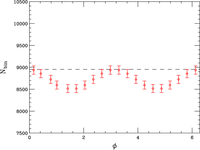
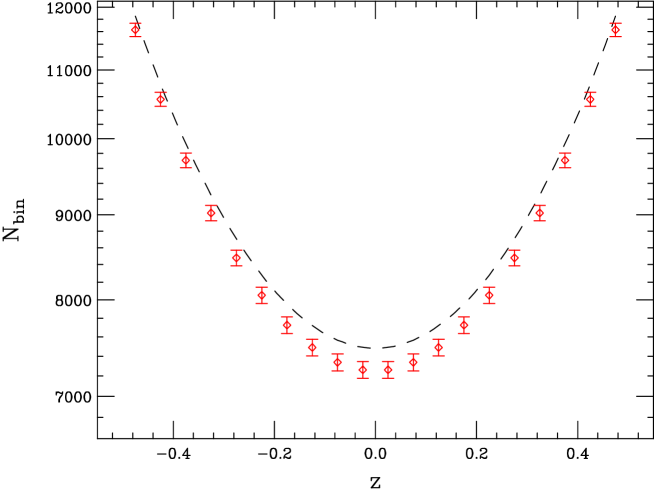
Figure 15: $\phi$ dependence (top) and $\theta$ dependence (bottom) of the $e^{+}e^{-}\rightarrow\gamma\gamma$ cross section for the case $\alpha=\pi/2$. We take $\Lambda_{NC}={\sqrt{s}}=500$ GeV, and assume a luminosity of $500\,{\rm fb}^{-1}$. In the top panel a cut of $|z|<0.5$ has been employed. The dashed line corresponds to the SM expectations and the ‘data’ points represent the NCQED results.

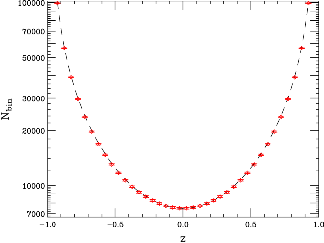
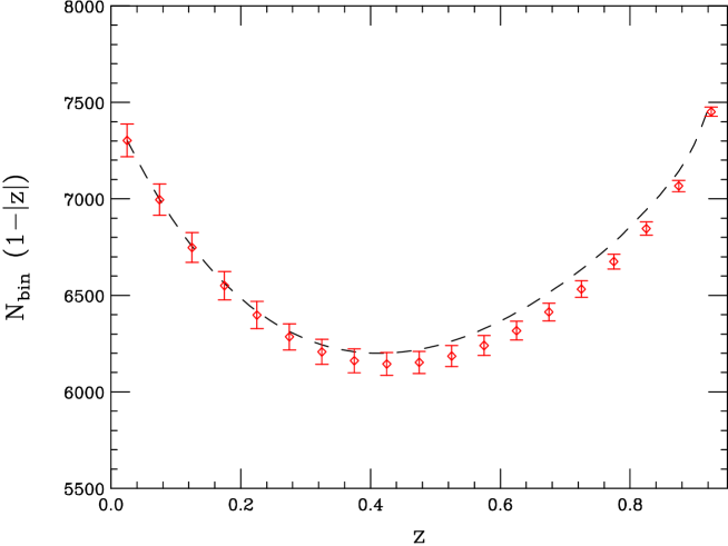
Figure 16: $\theta$ dependence of the $e^{+}e^{-}\rightarrow\gamma\gamma$ cross section for the case $\alpha=0$. We again use $\Lambda_{NC}={\sqrt{s}}=500$ GeV, and a luminosity of $500\,{\rm fb}^{-1}$. In the bottom panel, note that the number of events in each bin is scaled by $1-|z|$.

In Figs. 15 and 16 we present the bin-integrated event rates, taking $\Lambda_{NC}=\sqrt{s}$ for purposes of demonstration, which show the angular dependences of the NC deviations for the two cases $\alpha=\pi/2$ and $\alpha=0$, taking $\Lambda_{NC}={\sqrt{s}}=500$ GeV and a luminosity of $500\,{\rm fb}^{-1}$. For the case of $\alpha=0$ we have also scaled the angular distribution by the factor $1-|z|$ in order to emphasize the deviation from the Standard Model in the peaking region. Note that the NC contributions lower the event rate from that expected in the SM in the central region. As expected, the $\alpha=0$ case shows no $\phi$ dependence since the preferred direction is parallel to the beam axis, while the $\phi$ distribution for $\alpha=\pi/2$ exhibits a strong oscillatory behavior. The case $\alpha=\pi/4$, as well as more general choices of $\alpha$, simply extrapolates between these two extremes.

To obtain a 95% CL lower bound on $\Lambda_{NC}$, we perform a fit to the total cross section and the angular distributions employing the procedure discussed above. Our results are presented in Fig. 17 for three values of $\alpha$, where we see that the NC search reach from pair annihilation is approximately given by $1.5\sqrt{s}$. This is inferior in comparison to that obtained in the case of Moller and Bhabha scattering, due, in part, to the large available statistics in the latter cases. The scaled cross sections, after employing identical $z$ cuts as in the previous two sections, are presented in Fig. 18. Here, we see again that the anticipated high energy behavior is realized.

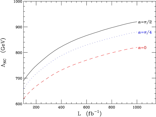
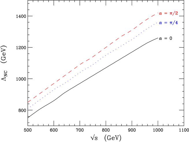
Figure 17: $95\%$ CL bound on $\Lambda_{NC}$ from pair annihilation as a function of luminosity (top) and ${\sqrt{s}}$ (bottom). In the top panel we set ${\sqrt{s}}=500$ GeV, while in the bottom panel we assume a luminosity of $500\,{\rm fb}^{-1}$.

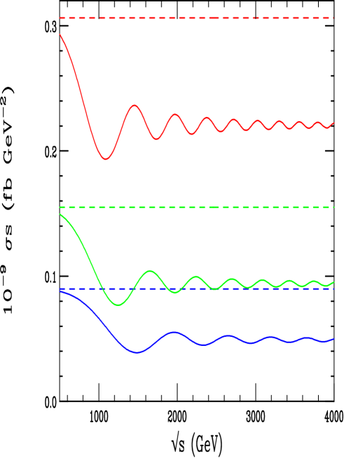
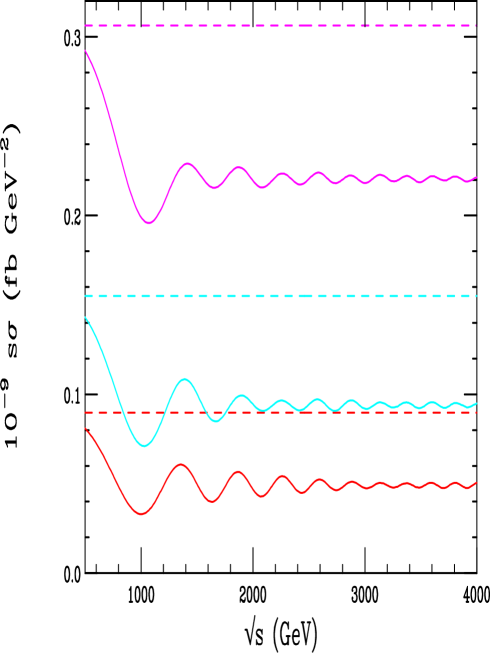
Figure 18: The scaled cross section for pair annihilation for $\alpha=0,\pi/2$ corresponding to the (top, bottom) panels, respectively.

5 $\gamma\gamma\rightarrow\gamma\gamma$ at Linear Colliders

Future linear colliders have the option of running in a photon-photon collision mode[22], in which laser photons are Compton back-scattered off the incoming fermion beams. The lowest order SM contributions arise at the 1-loop level with fermions and $W$ bosons propagating in the loop. Since the exact SM calculation of this box diagram mediated process is rather tedious[23], there exist various approximations in the literature[24] which are valid in the regime where the center of mass energy is large compared to the $W$ mass. Since this process only occurs at loop-level in the SM, it has been proposed as a useful test of new physics which contributes to the amplitude at the tree level in, for example, supersymmetry[24] or quantum gravity models with large extra dimensions[25]. In the present case, NCQED also predicts new contributions to $\gamma\gamma\rightarrow\gamma\gamma$ at tree-level, and hence we examine how well this process can bound $\Lambda_{NC}$.

We will consider only tree-level NC contributions since the NC generalization of the full electroweak SM is unknown and coupling constant suppressed. There are four diagrammatic contributions in this case: three from the $s$, $t$, and $u$ channels of photon exchange and one from the four-point photon coupling. These are presented in Fig. 19. Denoting the incoming photon momenta by $p_{1}$ and $p_{2}$, and the outgoing photon momenta by $k_{1}$ and $k_{2}$ as before, we find six non-vanishing NC helicity amplitudes:

$${\cal M}_{+--+}^{NC} = -32\pi\alpha\,\frac{\hat{t}}{\hat{s}}\,\bigg{[}\,{\rm sin}(\frac{1}{2}p_{1}\wedge k_{1})\,{\rm sin}(\frac{1}{2}p_{2}\wedge k_{2})+\frac{\hat{t}}{\hat{u}}\,{\rm sin}(\frac{1}{2}p_{1}\wedge k_{2})\,{\rm sin}(\frac{1}{2}p_{2}\wedge k_{1})\bigg{]}$$

$${\cal M}_{++++}^{NC} = 32\pi\alpha\,\bigg{[}\,\frac{\hat{u}-\hat{t}}{\hat{s}}\,{\rm sin}(\frac{1}{2}p_{1}\wedge p_{2})\,{\rm sin}(\frac{1}{2}k_{1}\wedge k_{2})\,+\,\bigg{(}\frac{\hat{u}}{\hat{t}}-\frac{2\hat{u}}{\hat{s}}\bigg{)}\,{\rm sin}(\frac{1}{2}p_{1}\wedge k_{1})$$ (30)

$$\times\,{\rm sin}(\frac{1}{2}p_{2}\wedge k_{2})+\,\bigg{(}\frac{\hat{t}}{\hat{u}}-\frac{2\hat{t}}{\hat{s}}\bigg{)}\,{\rm sin}(\frac{1}{2}p_{1}\wedge k_{2})\,{\rm sin}(\frac{1}{2}p_{2}\wedge k_{1})\bigg{]},$$

where we have made use of the relation $\hat{s}+\hat{t}+\hat{u}=0$ and the $\hat{s}$ denotes the parton-level center-of-mass frame. The other four amplitudes are related to these by ${\cal M}_{----}^{NC}={\cal M}_{++++}^{NC}$; $\,{\cal M}_{+--+}^{NC}(k_{1},k_{2})={\cal M}_{-++-}^{NC}(k_{1},k_{2})={\cal M}_{+-+-}^{NC}(k_{2},k_{1})={\cal M}_{-+-+}^{NC}(k_{2},k_{1})$. The corresponding SM amplitudes can be found in Refs. [24, 25] and will be given in the appendix.

Figure 19: The tree level contributions to $\gamma\gamma\rightarrow\gamma\gamma$ in NCQED.

The kinematics of this process are more complicated than those of the previous cases. The backscattered photons have a broad energy distribution, and the collision no longer occurs in the center of mass frame, i.e., the CM and laboratory frames no longer coincide. As NC theories violate Lorentz invariance, the differential cross section is no longer invariant under boosts along the z-axis and we are thus forced to consider this process in the laboratory frame. Letting $x_{1}$ and $x_{2}$ denote the fraction of the fermion energy carried by each of the backscattered photons, the photon momenta become

$$p_{1}^{\mu} = \frac{x_{1}{\sqrt{s}}}{2}(1,1,0,0)$$

$$p_{2}^{\mu} = \frac{x_{2}{\sqrt{s}}}{2}(1,-1,0,0)$$

$$k_{1}^{\mu} = E_{1}(1,c_{\theta},s_{\theta}c_{\phi},s_{\theta}s_{\phi})$$

$$k_{2}^{\mu} = ((x_{1}+x_{2})\frac{{\sqrt{s}}}{2}-E_{1},(x_{1}-x_{2})\frac{{\sqrt{s}}}{2}-E_{1}c_{\theta},-E_{1}s_{\theta}c_{\phi},-E_{1}s_{\theta}s_{\phi})\,,$$ (31)

where $E_{1}$ is given by

$$E_{1}=\frac{x_{1}x_{2}{\sqrt{s}}}{x_{1}+x_{2}-(x_{1}-x_{2})\,{\rm cos}\theta}\,.$$ (32)

Note that the Mandelstam invariants appearing in the amplitudes are now those for the photon-photon center of mass frame, with, e.g., $\sqrt{\hat{s}}=x_{1}x_{2}\sqrt{s}$.

We define the observable amplitudes by summing over the helicities of the outgoing photons:

$$|{\cal M}_{++}|^{2} = \sum_{ij}|{\cal M}_{++ij}|^{2}\,,$$

$$|{\cal M}_{+-}|^{2} = \sum_{ij}|{\cal M}_{+-ij}|^{2}\,,$$ (33)

which also include the SM contributions. The lab frame differential cross section for this process is

$$\frac{d\sigma}{d\Omega} = \frac{1}{128\pi^{2}s}\,\int\,\int\,dx_{1}\,dx_{2}\,\frac{E_{1}}{E_{2}}\,\frac{f(x_{1})f(x_{2})}{x_{1}x_{2}}\,\bigg{[}\bigg{(}\frac{1+\xi(x_{1})\xi(x_{2})}{2}\bigg{)}\,|M_{++}|^{2}\,$$ (34)

$$+\,\bigg{(}\frac{1-\xi(x_{1})\xi(x_{2})}{2}\bigg{)}\,|M_{+-}|^{2}\,\bigg{]}\,,$$

where $E_{1},\,\,E_{2}$ denote the outgoing photon energies, $f(x)$ is the photon number density function, and $\xi(x)$ the helicity distribution function, which is presented in the appendix. The distribution functions depend upon the variable set $(P_{e1},\,P_{l1},\,P_{e2},\,P_{l2})$, which represent the polarizations of the initial fermion and laser beams. In this paper we set $|P_{e}|=0.9$ and $|P_{l}|=1.0$, leaving six independent combinations: $(+,\,+,\,+,\,+),$ $\,(+,\,+,\,+,\,-),$ $(+,\,+,\,-,\,-),$ $(+,\,-,\,+,\,-),$ $(-,\,+,\,+,\,-),$ and $(+,$ $\,-,\,-,\,-),$ where, for example, $(+,\,-,\,+,\,-)$ means $P_{e1}=0.9$, $P_{l1}=-1.0$, $P_{e2}=0.9$, and $P_{l2}=-1.0$. We use the approximate SM amplitudes found in [24, 25], valid for $m_{W}^{2}/x_{p}\,<1$, where $x_{p}$ represents any of the photonic Mandelstam invariants. To validate this approximation we employ the cuts

$$|{\rm cos}(\theta)|\,\leq\,0.8\,,\;\;\;\;{\sqrt{0.4}}\,<\,x_{i}\,<\,x_{max}\,.$$ (35)

$x_{max}$ is the maximum fraction of the fermion beam energy that a backscattered photon can carry away; numerically, $x_{max}\approx 0.83$. Evaluating the wedge products in the NC amplitudes in the lab frame yields

$$p_{1}\wedge p_{2} = \frac{-c_{01}x_{1}x_{2}s}{2\Lambda^{2}_{NC}}$$

$$p_{1}\wedge k_{1} = \frac{-x_{1}E_{1}{\sqrt{s}}}{2\Lambda^{2}_{NC}}\,\bigg{[}\,c_{01}\,(1-c_{\theta})-c_{02}s_{\theta}c_{\phi}-c_{03}s_{\theta}s_{\phi}-c_{12}s_{\theta}c_{\phi}+c_{31}s_{\theta}s_{\phi}\,\bigg{]}$$

$$p_{2}\wedge k_{1} = \frac{x_{2}E_{1}{\sqrt{s}}}{2\Lambda^{2}_{NC}}\,\bigg{[}\,c_{01}\,(1+c_{\theta})+c_{02}s_{\theta}c_{\phi}+c_{03}s_{\theta}s_{\phi}-c_{12}s_{\theta}c_{\phi}+c_{31}s_{\theta}s_{\phi}\,\bigg{]}$$

$$p_{1}\wedge k_{2} = \frac{-x_{1}E_{1}{\sqrt{s}}}{2\Lambda^{2}_{NC}}\,\bigg{[}\,\frac{c_{01}x_{2}{\sqrt{s}}}{E_{1}}-c_{01}(1-c_{\theta})+c_{02}s_{\theta}c_{\phi}+$$

$$c_{03}s_{\theta}s_{\phi}+c_{12}s_{\theta}c_{\phi}-c_{31}s_{\theta}s_{\phi}\,\bigg{]}$$

$$p_{2}\wedge k_{2} = \frac{-x_{2}E_{1}{\sqrt{s}}}{2\Lambda^{2}_{NC}}\,\bigg{[}\,\frac{-c_{01}x_{1}{\sqrt{s}}}{E_{1}}+c_{01}(1+c_{\theta})+c_{02}s_{\theta}c_{\phi}+$$

$$c_{03}s_{\theta}s_{\phi}-c_{12}s_{\theta}c_{\phi}+c_{31}s_{\theta}s_{\phi}\,\bigg{]}$$

$$k_{1}\wedge k_{2} = \frac{-E_{1}{\sqrt{s}}}{2\Lambda^{2}_{NC}}\,\bigg{[}\,(x_{1}+x_{2})\{c_{02}s_{\theta}c_{\phi}+c_{03}s_{\theta}s_{\phi}+c_{01}c_{\theta}\}$$ (36)

$$-(x_{1}-x_{2})\{c_{01}-c_{12}s_{\theta}c_{\phi}+c_{31}s_{\theta}s_{\phi}\}\bigg{]},$$

where, as before, we can interpret the $c_{\mu\nu}$ in terms of the directions of the background $E$ and $B$ fields, with, the z-axis has being defined to be along the direction of the initial beams. Note that in this case, however, we have defined $p_{1}$ to be in the positive z-direction. Two important properties of these expressions are that the presence of both $c_{0i}$ and $c_{ij}$ indicates that $\gamma\gamma\rightarrow\gamma\gamma$ is sensitive to both space-time and space-space non-commutativity, unlike the previously examined processes, and the disappearance of $c_{23}$ indicates that B fields parallel to the beam axis are unobservable as in the case of Moller scattering. We consider three different possibilities: (i) $c_{01}=1$, with all others vanishing; (ii) $c_{03}=1$, with all others vanishing; and (iii) $c_{12}=-1$, with all others vanishing. In terms of the angular parameterization, case (i) corresponds to an E field parallel to the beam axis (denoted by $\alpha=0$ in our discussion of $e^{+}e^{-}\rightarrow\gamma\gamma$), case (ii) to an E field perpendicular to the beam axis ($\alpha=\pi/2$ in $e^{+}e^{-}\rightarrow\gamma\gamma$), and case (iii) to a B field perpendicular to the beam axis. As noted earlier for $e^{+}e^{-}\rightarrow\gamma\gamma$, $c_{02}$ and $c_{03}$ are equivalent up to a redefinition of $\phi$, as are $c_{12}$ and $c_{31}$. Note, however, that despite their apparent similarity, the space-time and space-space components are not equivalent up to a redefinition of $\phi$. Redefining $\phi$ in an attempt to relate $c_{03}$ and $c_{12}$ inflicts a sign change in the amplitudes, which affects the interference between the SM and NC amplitudes.

In Figs. 20, 21, and 22 we display the bin-integrated angular distributions assuming a 500 GeV $e^{+}e^{-}$ linear collider with an integrated luminosity of $500\,{\rm fb}^{-1}$ and employing the cuts discussed above. We also take $\Lambda_{NC}=\sqrt{s}$ for purposes of demonstration. As can be seen from the figures, the effects of NC space-time yield marked increases in both the $z$ and $\phi$ distributions over the SM expectations, whereas this process is seen to be rather insensitive to space-space non-commutativity. The NC space-space corrections also do not strictly increase the SM result, unlike the other two cases, due to an interference effect between the SM and space-space NC contributions, and from the small magnitude of the NC effect in this case.

Figure 23 displays the $95\%$ CL search reach for the NC scale $\Lambda_{NC}$ as a function of luminosity for the three cases with the polarization state $(+,-,+,-)$ as well as for the case $c_{01}$ with all polarization configurations. As expected, $\gamma\gamma$ scattering is relatively insensitive to space-space non-commutativity yielding bounds that are essentially just below $\sqrt{s}$. However, in the case of space-time NC, we see that the potential limits are comparable to that obtainable from pair annihilation and are of order $1.5\sqrt{s}$. 2 photon scattering also nicely complements $e^{+}e^{-}\rightarrow\gamma\gamma$ as one is sensitive to $c_{01}$ with the other depending on $c_{02}$ and $c_{03}$.

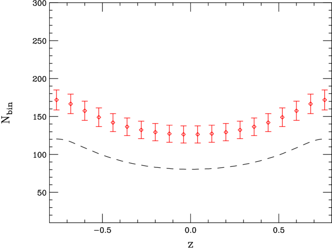
Figure 20: Angular dependence of the $\gamma\gamma\rightarrow\gamma\gamma$ cross section for the case $c_{01}=1$. We take $\Lambda_{NC}={\sqrt{s}}=500$ GeV, and a luminosity of $500\,{\rm fb}^{-1}$ and employ the cuts discussed in the text.

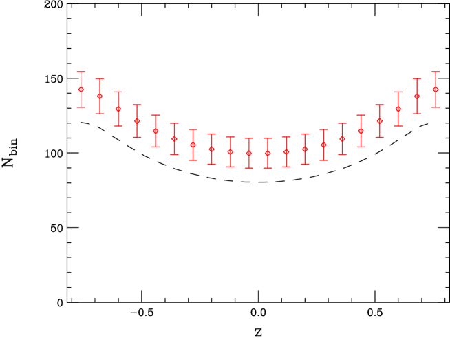
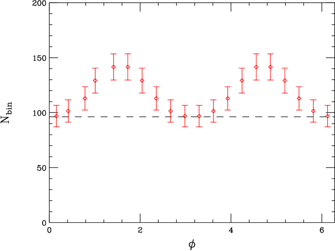
Figure 21: $\theta$ (top) and $\phi$ dependence (bottom) of the $\gamma\gamma\rightarrow\gamma\gamma$ cross section for the case $c_{03}=1$. We again take $\Lambda_{NC}={\sqrt{s}}=500$ GeV, with a luminosity of $500\,{\rm fb}^{-1}$.

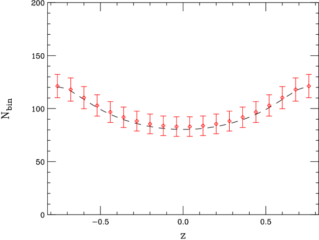
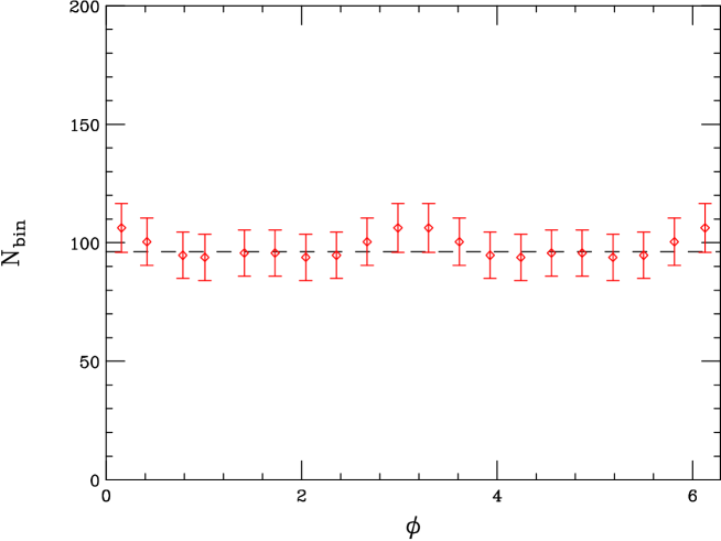
Figure 22: Same as the previous figure, only for $c_{12}=-1$.

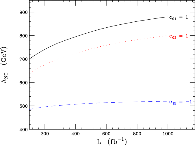
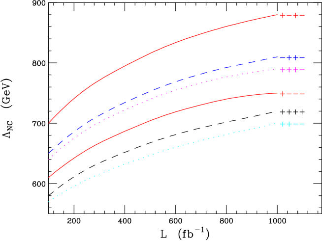
Figure 23: $95\%$ CL bound on $\Lambda_{NC}$ from $\gamma\gamma\rightarrow\gamma\gamma$ as a function of luminosity for ${\sqrt{s}}=500$ GeV. Top panel: the three cases of $c_{\mu\nu}$ discussed in the text with the polarization state $(+,-,+,-)$, and bottom panel: all polarization states with $c_{01}=1$.

6 Conclusions

In summary, we have examined the testable nature of non-commutative quantum field theory by analyzing various $2\rightarrow 2$ processes at high energy $e^{+}e^{-}$ linear colliders. We have parameterized the non-commutative relationship in terms of an overall NC scale, $\Lambda_{NC}$, and an anti-symmetric matrix $c_{\mu\nu}$ which is related to the direction of the background electromagnetic field present in these theories. We have seen that these theories give rise to modifications to QED, resulting in a non-abelian like nature with 3- and 4-point photon self-couplings, as well as momentum dependent phase factors appearing at each possible vertex in NCQED. We have seen that both Bhabha and Moller scattering are affected by the interference momentum dependent phase factors, whereas pair annihilation also receives contributions from the 3-point function. We have also examined $\gamma\gamma\rightarrow\gamma\gamma$, which is sensitive to both the 3- and 4-photon self-couplings.

In all the processes considered in the text, the NC affects arise at lowest order from dimension-8 operators. In addition, they generate an azimuthal dependence, which is not present in the SM, due to the NC preferred direction in space-time. These effects are not Lorentz invariant, and caution must be exercised in evaluating them, both theoretically and experimentally.

The above four processes are complementary in terms of probing the NC parameter space. Pair annihilation and Bhabha scattering, together, explore the full parameter space for Space-Time non-commutativity, whereas Moller scattering is sensitive to 2 of the parameters in the case of Space-Space NC. Two photon scattering simultaneously probes Space-Space and Space-Time NC, but is found to be rather insensitive numerically to the Space-Space case. In all of these transitions, the effects of B fields parallel to the beam axis are unobservable. We summarize our results for the $95\%$ CL search reach for the NC scale in Table 1. We see that NCQED can be probed to scales of order a TeV, which is where one would expect NCQFT to become important, if stringy effects or if the fundamental Planck scale are also at the TeV scale.

Process	Structure Probed	Bound on $\Lambda_{NC}$
$e^{+}e^{-}\rightarrow\gamma\gamma$	Space-Time	$740-840$ GeV
Moller Scattering	Space-Space	1700 GeV
Bhabha Scattering	Space-Time	1050 GeV
$\gamma\gamma\rightarrow\gamma\gamma$	Space-Time	$700-800$ GeV
	Space-Space	500 GeV

Table 1: Summary of the $95\%$ CL search limits on the NC scale $\Lambda_{NC}$ from the various processes considered above at a 500 GeV $e^{+}e^{-}$ linear collider with an integrated luminosity of 500  ${\mathrm{fb}}^{-1}$.

Note Added: While this paper was being completed, a related work [26] appeared. There is some overlap between the processes considered in this paper with what is contained here, however, we disagree completely with their results. We also note that crossing symmetry can be maintained in NCQFT as long as one exercises care to also switch the appropriate momenta in the wedge products.

Acknowledgements

The authors would like to thank D. Atwood, H. Davoudiasl, and A. Kronfeld for discussions. TGR thanks S. Gardner at the University of Kentucky for the use of facilities. F. P. was supported in part by a NSF Graduate Research Fellowship.

Appendix

In this appendix we present the SM amplitudes and photon distribution functions relevant for the process $\gamma\gamma\rightarrow\gamma\gamma$. For a more detailed discussion the reader is referred to [22, 23, 24, 25].

As discussed in the text, the one loop contributions to $\gamma\gamma\rightarrow\gamma\gamma$ arise from $W$ boson and fermion loops. At high energies, which we are considering, there is only one non-negligible independent helicity amplitude. The approximate amplitudes for the $W$ contribution is

$$\frac{{\cal M}_{++++}^{(W)}(s,t,u)}{\alpha^{2}}\approx 12+12\left(\frac{u-t}{s}\right)\left[\ln\left(\frac{-u-i\varepsilon}{m_{W}^{2}}\right)-\ln\left(\frac{-t-i\varepsilon}{m_{W}^{2}}\right)\right]$$

$$+16\left(1-\frac{3tu}{4s^{2}}\right)\left(\left[\ln\left(\frac{-u-i\varepsilon}{m_{W}^{2}}\right)-\ln\left(\frac{-t-i\varepsilon}{m_{W}^{2}}\right)\right]^{2}+\pi^{2}\right)$$

$$+16s^{2}\left[\frac{1}{st}\ln\left(\frac{-s-i\varepsilon}{m_{W}^{2}}\right)\ln\left(\frac{-t-i\varepsilon}{m_{W}^{2}}\right)+\frac{1}{su}\ln\left(\frac{-s-i\varepsilon}{m_{W}^{2}}\right)\ln\left(\frac{-u-i\varepsilon}{m_{W}^{2}}\right)\right.$$

$$+\left.\frac{1}{tu}\ln\left(\frac{-t-i\varepsilon}{m_{W}^{2}}\right)\ln\left(\frac{-u-i\varepsilon}{m_{W}^{2}}\right)\right],$$ (37)

where $\alpha\approx 1/137$, $m_{W}$ represents the mass of the $W$ boson and $\varepsilon$ is a small positive quantity defining the branch cut prescription. The fermion contribution gives rise to the approximate amplitude

$$\frac{{\cal M}_{++++}^{(f)}(s,t,u)}{\alpha^{2}Q_{f}^{4}}\approx-8-8\left(\frac{u-t}{s}\right)\left[\ln\left(\frac{-u-i\varepsilon}{m_{f}^{2}}\right)-\ln\left(\frac{-t-i\varepsilon}{m_{f}^{2}}\right)\right]$$

$$-4\left(\frac{t^{2}+u^{2}}{s^{2}}\right)\left(\left[\ln\left(\frac{-u-i\varepsilon}{m_{f}^{2}}\right)-\ln\left(\frac{-t-i\varepsilon}{m_{f}^{2}}\right)\right]^{2}+\pi^{2}\right),$$ (38)

where $Q_{f}$ is the fermion charge in units of the positron charge, and $m_{f}$ is the mass of the fermion in the loop. The other amplitudes are related to these by

$${\cal M}_{+-+-}(s,t,u)\,=\,{\cal M}_{+--+}(s,u,t)\,=\,{\cal M}_{++++}(u,t,s).$$ (39)

We now present the expressions for the photon distributions. We define the auxiliary functions

$$C(x)\equiv\frac{1}{1-x}+(1-x)-4r(1-r)-P_{e}\,P_{l}\,r\,z(2r-1)(2-x),$$ (40)

where $r=x/[z(1-x)]$, and

$$\sigma_{{}_{C}}=\left(\frac{2\pi\alpha^{2}}{m_{e}^{2}z}\right)\left[\left(1-\frac{4}{z}-\frac{8}{z^{2}}\right)\ln(z+1)+\frac{1}{2}+\frac{8}{z}-\frac{1}{2(z+1)^{2}}\right]$$

$$+P_{e}\,P_{l}\left(\frac{2\pi\alpha^{2}}{m_{e}^{2}z}\right)\left[\left(1+\frac{2}{z}\right)\ln(z+1)-\frac{5}{2}+\frac{1}{z+1}-\frac{1}{2(z+1)^{2}}\right].$$ (41)

Here $z$ is a variable describing the laser photon energy; varying $z$ affects the value of $x_{max}$, the maximum value of the fermion beam energy that the backscattered photons can acquire. We set $z=2(1+{\sqrt{2}})$ in our analysis, which maximizes $x_{max}$. In terms of these functions the photon number and helicity distribution functions take the form

$$f(x,P_{e},P_{l};z) = \left(\frac{2\pi\alpha^{2}}{m_{e}^{2}z\sigma_{{}_{C}}}\right)C(x)$$ (42)

$$\xi(x,P_{e},P_{l};z) = \frac{1}{C(x)}\left\{P_{e}\,\left[\frac{x}{1-x}+x(2r-1)^{2}\right]-P_{l}\,(2r-1)\left(1-x+\frac{1}{1-x}\right)\right\}\,.$$

References

- [1] For a review see, J.L. Hewett and T.G. Rizzo, Phys. Rep. 183, 193 (1989).
- [2] There is a large literature on this subject; see for example, N. Arkani-Hamed, S. Dimopoulos, and G. Dvali, Phys. Lett. B429, 263 (1998), and Phys. Rev. D59, 086004 (1999); I. Antoniadis, N. Arkani-Hamed, S. Dimopoulos, and G. Dvali, Phys. Lett. B436, 257 (1998); L. Randall and R. Sundrum, Phys. Rev. Lett. 83, 3370 (1999), and ibid., 4690, (1999); I. Antoniadis, Phys. Lett. B246, 377 (1990); I. Antoniadis, C. Munoz and M. Quiros, Nucl. Phys. B397, 515 (1993); I. Antoniadis and K. Benalki, Phys. Lett. B326, 69 (1994); I. Antoniadis, K. Benalki and M. Quiros, Phys. Lett. B331, 313 (1994); J. Lykken, Phys. Rev. D54, 3693 (1996); E. Witten, Nucl. Phys. B471, 135 (1996); P. Horava and E. Witten, Nucl. Phys. B460, 506 (1996) and Nucl. Phys. B475, 94 (1996).
- [3] A. Connes, Non-commutative Geometry, Academic Press, 1994; J. Gomis, M. Kleban, T. Mehen, M. Rangamani and S. Shenker, hep-th/0003215; E.T. Akhmedov, P. DeBoer and G.W. Semenoff, hep-th/0010003; A. Rajaraman and M. Rozali, hep-th/0003227; J. Gomis, T. Mehen and M.B. Wise, hep-th/0006160; J.W. Moffat, hep-th/0007181; F. Lizzi, G. Mangano and G. Miele, hep-th/0009180; J. Gomis, K. Kamimura and T. Mateos, hep-th/0009158.
- [4] V.A. Kostelecky and S. Samuel, Phys. Rev. Lett. 63, 224 (1989), Phys. Rev. Lett. 66, 1811 (1991), Phys. Rev. D39, 683 (1989), and Phys. Rev. D40, 1886 (1990); V.A. Kostelecky and R. Potting, Nucl. Phys. B359, 545 (1991) and Phys. Lett. B381, 89 (1996); S. Coleman and S.L. Glashow, Phys. Rev. D59, 116008 (1999); J. Ellis, N.E. Mavromatos and D.V. Nanopoulos, gr-qc/0005100.
- [5] N. Seiberg and E. Witten, J. High Energy Phys. 9909, 032 (1999), hep-th/9908142; M.R. Douglas and C. Hull, J. High Energy Phys. 9802, 008 (1998), hep-th/9711165; A. Connes, M.R. Douglas and A. Schwarz, J. High Energy Phys. 9802, 003 (1998), hep-th/9711162; N. Seiberg, L. Susskind and N. Toumbas, hep-th/0005040; R. Gopakumar, J. Maldacena, S. Minwalla and A. Strominger, hep-th/0005048; S. Jabbari, Phys. Lett. B455, 129 (1999); D. Bigatti and L. Susskind, hep-th/9908056; T. Pengpan and X. Xiong, hep-th/0009070; D.J. Gross, A. Hashimoto and N. Itzhaki, hep-th/0008075; J.L.F. Barbon and E. Rabinovici, hep-th/0005073.
- [6] Here we follow a number of discussions in the literature; see for example, Ihab. F. Riad and M.M. Sheikh-Jabbari, hep-th/0008132.
- [7] M. Chaichian, A. Demichev, P. Pres̆najder and A. Tureanu, hep-th/0007156; O. Aharony, J. Gomis and T. Mehen, hep-th/0006236; J. Gomis and T. Mehen, hep-th/0005129; N. Seiberg, L. Susskind and N. Toumbas, hep-th/0005015; M. Chaichan, A. Demichev, and P. Pres̆najder, Nucl. Phys. B567, 360 (2000).
- [8] R.-G. Cai and N. Ohta, hep-th/0008119.
- [9] K. Matsubara, hep-th/0003294. See, however, L. Bonora, M. Schnabl, M.M. Sheikh-Jabbari, and A. Tomasiello, Nucl. Phys. B589, 461 (2000), where the star product expansion has been extended to NC SO(n) and Sp(n) theories.
- [10] L. Bonora and M. Salizzoni, hep-th/0011083; C.P. Martin and D. Sanchez-Ruiz, Phys. Rev. Lett. 83, 476 (1999); M.M. Sheikh-Jabbari, hep-th/9903107; S. Minwalla, M. Van Raamsdonk and N. Seiberg, hep-th/9912072; I.Chepelev, R. Roiban, hep-th/9911098; T. Krajewski and R. Wulkenhaar, hep-th/9903187; I. Ya. Aref’eva, D.M. Belov, and A.S. Koshelev, hep-th/0001215; A. Matusis, L. Susskind and T. Toumbas, hep-th/0002075; J.C. Varilly and J.M. Gracia-Bondia, Int. J. Mod. Phys. A14, 1305 (1999); H. Grosse, T. Krajewski and R. Wulkenhaar, hep-th/0001182; I. Ya. Aref’ava, D.M. Belov, and A.S. Koshelev, hep-th/0001215, and Phys. Lett. B476, 431 (2000), hep-th/9912075; T. Filk, Phys. Lett. B376, 53 (1996). See, however, A. Micu and M.M. Sheikh-Jabbari, hep-th/0008057, where it is shown that the NC parameter is not renormalized at two-loops in theory.
- [11] For a discussion see F.J. Petriello, hep-th/0101109, which disagrees with the results in B.A. Campbell and K. Kaminsky, hep-th/0101086, and hep-th/0003137.
- [12] M. Hayakawa, Phys. Lett. B478, 394 (2000).
- [13] Ihab. F. Riad and M.M. Sheikh-Jabbari, hep-th/0008132; F. Ardalan and N. Sadooghi, hep-th/0009233 and hep-th/0002143; C.P. Martin and D. Sanchez-Ruiz, Phys. Rev. Lett. 83, 476 (1999); N. Chair and M.M. Sheikh-Jabbari, hep-th/0009037; J.M. Gracia-Bondia and C.P. Martin, hep-th/0002171.
- [14] The Feynman rules for NCQED and more general non-commutative gauge theories can be found in: A. Armoni, hep-th/0005208; M.M. Sheikh-Jabbari, J. High Energy Phys. 9906, 015 (1999); T. Krajewski and R. Wulkenhaar, hep-th/9903187; I. Ya Aref’eva, D.M. Belov, A.S. Koshelev and O.A. Rytchkov, hep-th/0003176.
- [15] M.M. Sheikh-Jabbari, Phys. Rev. Lett. 84, 5265 (2000).
- [16] M. Chaichian, M.M. Sheikh-Jabbari, and A. Tureanu, hep-th/0010175.
- [17] See, for example, I. Mocioiu, M. Pospelov, and R. Roiban, Phys. Lett. B489, 390 (2000). This paper obtains strong bounds from considering linear NC effects in and a Lorentz violating term in a nucleon spin coupling to an external field, i.e., a nuclear Zeeman-like splitting. However, since NCQFT has yet to be extended to the full SM, it remains to be seen if these constraints would hold in a full theory.
- [18] G.F. Giudice, R. Rattazzi and J.D. Wells, Nucl. Phys. B544, 3 (1999); J.L. Hewett, Phys. Rev. Lett. 82, 4765 (1999); T.G. Rizzo, Phys. Rev. D59, 115010 (1999).
- [19] See the first two papers in Ref. 2.
- [20] See L. Randall and R. Sundrum in Ref. 2.
- [21] H. Davoudiasl, J.L. Hewett and T.G. Rizzo, Phys. Rev. Lett. 84, 2080 (2000) and hep-ph/0006041.
- [22] I. F. Ginzburg, G. L. Kotkin, V. G. Serbo and V. I. Telnov, Nucl. Instr. Methods 205 47 (1983); I. F. Ginzburg, G. L. Kotkin, S. L. Panfil, V. G. Serbo and V. I. Telnov, Nucl. Instr. Methods 219 5 (1984).
- [23] G. Jikia and A. Tkabladze, Phys. Lett. B323 453 (1994).
- [24] G. J. Gounaris, P. I. Porfyriadis, and F. M. Renard, Phys. Lett. B452 76 (1999), and Eur. Phys. J. C9 673 (1999).
- [25] H. Davoudiasl, Phys. Rev. D60 084022 (1999).
- [26] H. Arfaei and M.H. Yavartanoo, hep-th/0010244.