RM3-TH/00-17

ROMA-1297/00

First Lattice Calculation of the Electromagnetic Operator Amplitude $\langle\pi^{0}|Q_{\gamma}^{+}|K^{0}\rangle$
GLADIATOR The SPQcdR Collaboration Southampton-Paris-Rome
D. Becirevic^a, V. Lubicz^b, G. Martinelli^a and F. Mescia^a
a Dip. di Fisica, Univ. di Roma “La Sapienza” and INFN, Sezione di Roma,
Piazzale Aldo Moro 2, I-00185 Rome, Italy.
^b Dip. di Fisica, Univ. di Roma Tre and INFN, Sezione di Roma Tre,
Via della Vasca Navale 84, I-00146 Rome, Italy.

Abstract:
We present the first lattice calculation of the matrix element of the electromagnetic operator $\langle\pi^{0}|Q_{\gamma}^{+}|K^{0}\rangle$, where $Q_{\gamma}^{+}=(Q_{d}e/16\pi^{2})\left({\bar{s}}_{L}\sigma^{\mu\nu}F_{\mu\nu}d_{R}+{\bar{s}}_{R}\sigma^{\mu\nu}F_{\mu\nu}d_{L}\right)$. This matrix element plays an important rôle, since it contributes to enhance the CP violating part of the $K_{L}\to\pi^{0}e^{+}e^{-}$ amplitude in supersymmetric extensions of the Standard Model.

1 Introduction

The origin of CP violation is one of the fundamental questions of particle physics and cosmology which remains an open problem to date. The recent measurements of $\varepsilon^{\prime}/\varepsilon$ [1] have definitively established direct CP violation and ruled out superweak scenarios. Unfortunately, we are still far from a full quantitative description of the dynamics which generate the amount of CP violation observed in hadronic processes [2]. Given the large theoretical uncertainties affecting the calculation of $\varepsilon^{\prime}/\varepsilon$, it is very useful to collect additional experimental information about CP violation in different processes. The most interesting ones are those for which CP violating effects are suppressed in the Standard Model (SM) and enhanced in its extensions. Among the processes which have been considered in the literature, we like to mention charge asymmetries in non-leptonic decays [3, 4] and CP asymmetries of hyperon decays [5].

Good candidates to provide new large CP violating effects are the supersymmetric extensions of the SM with generic flavour couplings and minimal particle content. In this framework, among the possible contributions, it has been recently recognized the importance of the electromagnetic and chromomagnetic operators (EMO and CMO)

$$Q^{\pm}_{\gamma} = \frac{Q_{d}e}{16\pi^{2}}\left({\bar{s}}_{L}\sigma^{\mu\nu}F_{\mu\nu}d_{R}\pm{\bar{s}}_{R}\sigma^{\mu\nu}F_{\mu\nu}d_{L}\right)$$ (1)

$$Q^{\pm}_{g} = \frac{g}{16\pi^{2}}\left({\bar{s}}_{L}\sigma^{\mu\nu}t^{a}G^{a}_{\mu\nu}d_{R}\pm{\bar{s}}_{R}\sigma^{\mu\nu}t^{a}G^{a}_{\mu\nu}d_{L}\right)$$ (2)

The same mechanism, the misalignment between quark and squark mass matrices, may indeed substantially increase their CP-odd contribution to physical processes. In previous studies, particular attention has been devoted to the CMO which, without conflict with the experimental determination of the $K^{0}$–$\bar{K}^{0}$ mixing amplitude, can account for the largest part of the measured $\varepsilon^{\prime}/\varepsilon$ [6]–[9].

In this paper, we consider the CP violating contribution of the EMO to $K_{L}\to\pi^{0}e^{+}e^{-}$. The master formula which has been used in the numerical calculation of the rate is [4]

$${\rm B}(K_{L}\to\pi^{0}e^{+}e^{-})_{EMO}=5.3\times 10^{-4}\left(\frac{\tilde{y}_{\gamma}(m_{\tilde{g}},x_{gq})G_{0}(x_{gq})}{\tilde{y}_{\gamma}(500{\rm GeV},1)G_{0}(1)}\right)^{2}\tilde{B}_{T}^{2}\ (\mbox{Im}\delta_{+})^{2}\,.$$ (3)

The coupling $\delta_{+}$ is related to the splitting in the down-type squark mass matrix. The definitions of $\delta_{+}$ and $\tilde{y}_{\gamma}$ can be found in sec. 2 and $x_{gq}=m^{2}_{\tilde{g}}/m^{2}_{\tilde{q}}$ is the ratio of gluino and (average) squark mass squared. The numerical coefficient in eq. (3) is the appropriate one for the operator $Q_{\gamma}^{+}$ renormalized in $\overline{MS}$ at the scale $\mu=2$ GeV.

Our main result is the first lattice calculation of the $B$ parameter $\tilde{B}_{T}$ (also defined in sec. 2), for which we obtain

$$\tilde{B}^{\overline{MS}}_{T}(\mu=2{\rm GeV})=1.21\pm 0.09\pm 0.04^{+0.07}_{-0.00}\ ,$$ (4)

where the first error is the statistical one, the second is the systematic error due to the uncertainty on the ratio of the EMO to the vector current matrix elements and the third is the error coming from the uncertainty on the renormalization of the magnetic operator.

From the experimental upper bound [10]

$${\rm B}(K_{L}\to\pi^{0}e^{+}e^{-})<5.1\times 10^{-10}\,$$ (5)

by taking $\tilde{B}_{T}$ from eq. (4), $x_{gq}=1$ and $m_{\tilde{g}}=500$ GeV, and using eq. (3), we obtain

$$|\mbox{Im}\delta_{+}|<1.0\times 10^{-3}\quad\quad(95\,\%\ C.L.)$$ (6)

The remainder of the paper is organized as follows: in sec. 2 all the formulae necessary to derive eq. (3) are presented; in sec. 3 we describe the lattice simulation and discuss the calculation of $\tilde{B}_{T}$; sec. 4 contains our conclusion.

2 EMO Contribution to ${\rm B}(K_{L}\to\pi^{0}e^{+}e^{-})$

In this section, we recall the main ingredients necessary to compute ${\rm B}(K_{L}\to\pi^{0}e^{+}e^{-})$ in SUSY and introduce all the quantities appearing in eq. (3). We discuss separately the effective Hamiltonian and the calculation of the branching ratio.

2.1 The effective Hamiltonian for the magnetic operators

The supersymmetric contribution to the effective Hamiltonian, in the case of the magnetic operators, can be written as

$${\cal H}_{MO}=C_{\gamma}^{+}(\mu)Q_{\gamma}^{+}(\mu)+C_{\gamma}^{-}(\mu)Q_{\gamma}^{-}(\mu)+C_{g}^{+}(\mu)Q_{g}^{+}(\mu)+C_{g}^{-}(\mu)Q_{g}^{-}(\mu)\ ,$$ (7)

where the operators are renormalized at the scale $\mu$. The Wilson coefficients generated by gluino exchanges at the SUSY breaking scale are given by [9, 11]

$$C_{\gamma}^{\pm}(m_{\tilde{g}}) = \frac{\pi\alpha_{s}(m_{\tilde{g}})}{m_{\tilde{g}}}\left[\left(\delta^{D}_{LR}\right)_{21}\pm\left(\delta^{D}_{LR}\right)^{*}_{12}\right]F_{0}(x_{gq})\,,$$

$$C^{\pm}_{g}(m_{\tilde{g}}) = \frac{\pi\alpha_{s}(m_{\tilde{g}})}{m_{\tilde{g}}}\left[\left(\delta^{D}_{LR}\right)_{21}\pm\left(\delta^{D}_{LR}\right)^{*}_{12}\right]G_{0}(x_{gq})\,$$ (8)

Here $(\delta^{D}_{LR})_{ij}=(M^{2}_{D})_{i_{L}j_{R}}/m^{2}_{\tilde{q}}$ denote the off-diagonal entries of the (down-type) squark mass matrix in the super-CKM basis [12]. The explicit expressions of $F_{0}(x)$ and $G_{0}(x)$ are:

$$F_{0}(x) = \frac{4x\left(1+4x-5x^{2}+4x\ln\left(x\right)+2x^{2}\ln\left(x\right)\right)}{3(1-x)^{4}}\,,$$ (9)

$$G_{0}(x) = \frac{x\left(22-20x-2x^{2}+16x\ln\left(x\right)-x^{2}\ln\left(x\right)+9\ln\left(x\right)\right)}{3(1-x)^{4}}\ ,$$ (10)

with $F_{0}(1)=2/9$ and $G_{0}(1)=-5/18$. In the following we will use the combinations $\delta_{\pm}=(\delta_{LR}^{D})_{21}\pm(\delta_{LR}^{D})^{*}_{12}=(\delta_{LR}^{D})_{21}\pm(\delta_{RL}^{D})_{21}$. These quantities are the natural couplings appearing at first order in any parity conserving ($+$) or parity violating ($-$) observable.

In the $(Q_{\gamma}^{\pm},Q_{g}^{\pm})$ basis, using the leading order (LO) anomalous dimension matrix

$$\hat{\gamma}\ =\ \ \left(\begin{array}[]{cc}\frac{8}{3}&\;0\\ &\\ {{32}\over{3}}&\;{{4}\over{3}}\\ \end{array}\right)\ ,$$ (14)

it is straightforward to derive

$$C_{\gamma}^{\pm}(\mu) = \eta^{2}\left[C_{\gamma}^{\pm}(m_{\tilde{g}})+8(1-\eta^{-1})C_{g}^{\pm}(m_{\tilde{g}})\right]\ ,$$

$$C^{\pm}_{g}(\mu) = \eta\,C_{g}^{\pm}(m_{\tilde{g}})\,,$$ (15)

where

$$\eta=\left(\frac{\alpha_{s}(m_{\tilde{g}})}{\alpha_{s}(m_{t})}\right)^{2/21}\left(\frac{\alpha_{s}(m_{t})}{\alpha_{s}(m_{b})}\right)^{2/23}\left(\frac{\alpha_{s}(m_{b})}{\alpha_{s}(\mu)}\right)^{2/25}\ .$$ (16)

2.2 Calculation of ${\rm B}(K_{L}\to\pi^{0}e^{+}e^{-})$

In order to compute the rate, besides the Wilson coefficient, we also need the matrix element of the operator $Q^{+}_{\gamma}$, which is usually expressed in term of a suitable $B$ parameter [9]

$$\langle\pi^{0}|Q^{+}_{\gamma}|K^{0}\rangle=i\frac{Q_{d}e\sqrt{2}}{16\pi^{2}m_{K}}p_{\pi}^{\mu}p_{K}^{\nu}F_{\mu\nu}B_{T}{\cal R}_{T}(q^{2})\,.$$ (17)

With respect to the standard definition of $B_{T}$, we have introduced the $q^{2}$-dependent form factor ${\cal R}_{T}(q^{2})$ (${\cal R}_{T}(0)=1$) to account for the dependence of the matrix element on the momentum transfer $q=p_{K}-p_{\pi}$. Note that, since we are using renormalized operators, $B_{T}$ depends on both the renormalization scheme and scale.

Neglecting lepton masses, and isospin breaking effects, we may write the following useful identity

$$\frac{\langle\pi^{0}e^{+}e^{-}|Q^{+}_{\gamma}|K^{0}\rangle}{{\cal R}_{T}(q^{2})}=\frac{Q_{d}\alpha B_{T}}{4\pi m_{K}f^{+}(q^{2})}\langle\pi^{0}e^{+}\nu_{e}|(\bar{\nu}_{e}\gamma_{\mu}e)(\bar{s}\gamma^{\mu}u)|K^{+}\rangle\,,$$ (18)

where $\alpha$ is the electromagnetic coupling and $f^{+}(q^{2})=f^{+}(0){\cal R}_{+}(q^{2})$ is the vector current form factor defined as

$$\langle\pi^{0}|\bar{(}\bar{s}\gamma^{\mu}u)|K^{+}\rangle={1\over\sqrt{2}}\left[\left(p_{K}^{\mu}+p_{\pi}^{\mu}-\frac{m_{K}^{2}-m_{\pi}^{2}}{q^{2}}q^{\mu}\right)f^{+}(q^{2})+\frac{m_{K}^{2}-m_{\pi}^{2}}{q^{2}}q^{\mu}f^{0}(q^{2})\right]\ .$$ (19)

Eq. (18) allows us to write ${\rm B}(K_{L}\to\pi^{0}e^{+}e^{-})_{EMO}$ in terms of the $K^{+}$ semileptonic branching ratio

$${\rm B}(K_{L}\to\pi^{0}e^{+}e^{-})_{EMO}=2\left(\frac{\alpha}{2\pi}\right)^{2}{\rm B}(K^{+}\to\pi^{0}e^{+}\nu_{e})\frac{\tau(K_{L})}{\tau(K^{+})}\frac{|{\rm Im}\Lambda^{+}_{g}\tilde{y}_{\gamma}|^{2}}{|V_{us}|^{2}}\tilde{B}_{T}^{2}\,,$$ (20)

where we have followed the notation of ref. [9] by defining

$$\mbox{Im}\Lambda^{+}_{g}\tilde{y}_{\gamma}=\frac{Q_{d}}{\sqrt{2}G_{F}m_{K}}\mbox{Im}C^{+}_{\gamma}\ ,$$ (21)

with

$$\Lambda^{+}_{g}(x_{gq}) = \delta_{+}\ G_{0}(x_{gq})$$

$$\tilde{y}_{\gamma}(m_{\tilde{g}},x_{gq}) = \frac{\pi\alpha_{s}(m_{\tilde{g}})}{m_{\tilde{g}}}\frac{Q_{d}}{\sqrt{2}G_{F}m_{K}}\eta^{2}\left[\frac{F_{0}(x_{gq})}{G_{0}(x_{gq})}+8\left(1-\eta^{-1}\right)\right]\ .$$ (22)

The definition of $\tilde{y}_{\gamma}$ given above differs from that of ref. [9] by a factor $-B_{T}$, since it is preferable to separate the Wilson coefficient from the $B$ parameter.

We have introduced the “effective” $B$ parameter $\tilde{B}_{T}$ defined as

$$\tilde{B}_{T}=\frac{B_{T}}{f^{+}(0)}\times T\ ,\quad\quad T=\frac{\int_{0}^{(m_{K}-m_{\pi})^{2}}\,dq^{2}\lambda^{(3/2)}(q^{2})|{\cal R}_{T}(q^{2})|^{2}}{\int_{0}^{(m_{K}-m_{\pi})^{2}}\,dq^{2}\lambda^{(3/2)}(q^{2})|{\cal R}_{+}(q^{2})|^{2}}\ ,$$ (23)

where $\lambda(q^{2})=(m_{K}^{2}+m_{\pi}^{2}-q^{2})^{2}-4m_{K}^{2}m_{\pi}^{2}$. $T$ is the correction due to the different $q^{2}$ dependence of the tensor and vector form factors. In the calculation of $T$, we have used the experimental determination of the $q^{2}$ dependence of the semileptonic decay rate [13].

$${\cal R}_{+}(q^{2})=1+\frac{\lambda_{+}}{m_{\pi}^{2}}q^{2}\,,\quad\quad\lambda_{+}=0.0286\pm 0.0022$$ (24)

and the slope of the tensor form factor extracted from our lattice data (see sec. 3)

$${\cal R}_{T}(q^{2})=1+\frac{\lambda_{T}}{m_{\pi}^{2}}q^{2}\ ,\quad\quad\lambda_{T}=0.022\pm 0.001\,.$$ (25)

Since the correcting factor is very close to one, $T=0.99$, its effect is practically negligible for the value of the effective $B$ parameter, $\tilde{B}_{T}$. For the same reason, the difference between our value of $\lambda_{+}$ in eq. (25) and the experimental value of eq. (24) is ininfluential to the determination of $\tilde{B}_{T}$.

In order to compute $\tilde{B}_{T}$, we also need $B_{T}$ and $f^{+}(0)$. To wit, using the data discussed in sec. 3, we have followed two different procedures:

• we have taken the value $f^{+}(0)=0.978$ from ref. [14]. This number was obtained by neglecting isospin breaking effects. Using our result for the $B$ parameter, $B_{T}=1.23\pm 0.09$, and $T=0.99$, we get $\tilde{B}_{T}=1.25\pm 0.09$;

• we have computed on our data the ratio $B_{T}/f^{+}(0)$ extrapolated to the physical meson masses, obtaining $B_{T}/f^{+}(0)=1.18\pm 0.09$. With the same value of $T$ as before, in this case we get $\tilde{B}_{T}=1.17\pm 0.09$.

The difference between the two different procedures is taken into account in the systematic error, so that we get

$$\tilde{B}_{T}=1.21\pm 0.09\pm 0.04\ .$$ (26)

To this result, we add a very generous estimate ($+6\%$) of the systematic error (to be discussed in the next section) due to the renormalization of the EMO. In this way we arrive to the result quoted in eq. (4) of the introduction. This result is consistent with previous estimates from refs. [15, 16].

We have now all the necessary elements for the calculation of ${\rm B}(K_{L}\to\pi^{0}e^{+}e^{-})_{EMO}$. Using eq. (20), the definitions (22) and the values given in table 1, we arrive to the master formula in eq. (3) which has been used, together with $\tilde{B}_{T}$, to constrain ${\rm Im}\delta_{+}$.

lj Parameter	Value and error
$G_{F}$	$1.16639\times 10^{-5}\mbox{GeV}^{-2}$
$V_{us}$	$0.2196\pm 0.0023$
$m_{K}$	$0.498$ GeV
$m_{\pi}$	$0.135$ GeV
$\tau(K_{L})$	$(5.15\pm 0.04)\times 10^{-8}$ s
$\tau(K^{+})$	$(1.2385\pm 0.0025)\times 10^{-8}$ s
${\rm B}(K^{+}\to\pi^{0}e^{+}\nu_{e})$	$0.0485\pm 0.0009$
$\alpha_{s}(M_{Z})$	$0.119\pm 0.003$

Table 1: Average and errors of the main parameters. When the error is negligible it has been omitted.

3 Lattice calculation of the EMO matrix elements

In this section, we describe the procedure followed to obtain, in our lattice simulation, the $B$ parameter, $B_{T}$ ($f^{+}(0)$), and the form factor, ${\cal R}_{T}(q^{2})$ (${\cal R}_{+}(q^{2})$), necessary to the computation of ${\rm B}(K_{L}\to\pi^{0}e^{+}e^{-})_{EMO}$. Since the calculation of the form factors on the lattice has been discussed in several papers, see for example [17] and references therein, we only give here the details which characterize the present study.

All our lattice results have been obtained using a non-perturbatively improved action [18]. The relevant operators, namely the vector and tensor currents

$$\hat{V}_{\mu} = Z_{V}(1+b_{V}ma)\left[\bar{q}\gamma_{\mu}Q+ic_{V}\partial_{\nu}\bar{q}\sigma_{\mu\nu}Q\right]\ ,$$

$$\hat{T}_{\mu\nu} = Z_{T}(\mu)(1+b_{T}ma)\left[i\bar{q}\sigma_{\mu\nu}Q+c_{T}\left(\partial_{\nu}\bar{q}\gamma_{\mu}Q-\partial_{\mu}\bar{q}\gamma_{\nu}Q\right)\right]\ ,$$ (27)

are improved. In our study, the coefficient $b_{T}$, computed at ${\cal O}(\alpha_{s})$ [19], is evaluated by using boosted perturbation theory [20]. $Z_{T}(\mu)$ was obtained in ref. [21] with the non-perturbative method of ref. [22], in the RI-MOM scheme at the renormalization scale $\mu$. Note that for the tensor current, at the NLO, the RI-MOM scheme in the Landau gauge coincides with the $\overline{MS}$ scheme. The other constants are taken from the most recent non-perturbative determinations [23, 24]. In summary, we have used the following values

$$Z_{V}=0.79\ ,\ \quad b_{V}=1.4\ ,\ \quad c_{V}=-0.09\ ,$$ (28)

$$Z_{T}(\mu=2\ \mbox{GeV})=0.87\pm 0.01\ ,\ \quad b_{T}=1.2\ ,\ \quad c_{T}=0.05\ .$$

Since the perturbative value of $Z_{T}$ is $Z_{T}(\mu=2\ \mbox{GeV})=0.934(5)$, we estimate that the systematic error due to the normalization of the lattice operator is less than $6\,\%$. Also this effect is included in the evaluation of the systematic error.

Our analysis is based on a sample of $91$ independent quenched gauge-field configurations, generated at the lattice coupling constant $\beta=6/g_{0}^{2}=6.2$, on the volume $24^{3}\times 48$. We use the combination of values of the hopping parameter, $K_{L,l}$, which are given in tab. 2. In order to calibrate the lattice spacing, $a$, and to extrapolate the form factors to the physical meson masses, we use the lattice plane method [25]. We find $a^{-1}=2.7\pm 0.1$ GeV, in agreement with previous simulations.

3.1 Extraction of the form factor

Using standard lattice techniques, we have extracted from suitable correlation functions the matrix element of the operator

$$\langle\pi^{0}|\bar{s}\sigma^{\mu\nu}d|K^{0}\rangle=i\,\left(p_{K}^{\mu}p_{\pi}^{\nu}-p_{K}^{\nu}p_{\pi}^{\mu}\right)\frac{\sqrt{2}f_{T}(q^{2})}{m_{K}+m_{\pi}}\ ,$$ (29)

where we have introduced the form factor $f_{T}(q^{2})$ to make contact with the definition used in ref. [17]. From eq. (17), one finds

$$\frac{2f_{T}(q^{2})}{m_{K}+m_{\pi}}=\frac{B_{T}{\cal R}_{T}(q^{2})}{m_{K}}\ ,$$ (30)

so that $f_{T}(0)=B_{T}$ for $m_{K}=m_{\pi}$ corresponding to degenerate quark masses, $m_{s}=m_{u,d}$.

Besides $f_{T}(q^{2})$, we have also considered the vector form factors $f^{+}(q^{2})$ and $f^{0}(q^{2})$ ($f^{+}(0)=f^{0}(0)$) appearing in eq. (19). $f_{T}(q^{2})$, $f^{+}(q^{2})$ and $f^{0}(q^{2})$ have been computed for $\vec{p}_{K}=0$ at several values of the pion momentum, $\vec{p}_{\pi}=(2\pi/L)(n_{x},n_{y},n_{z})$ in lattice units. We have results for $(n_{x},n_{y},n_{z})=(0,0,0)$, $(1,0,0)$, $(2,0,0)$, $(1,1,0)$, $(1,1,1)$ and $(1,2,0)$. The results for $f_{T}(q^{2})$ as a function of the dimensionless variable $q^{2}a^{2}$ are shown in fig. 1.

Figure 1: $f_{T}(q^{2})$ as a function of $q^{2}$ for $K_{L}=K_{l}=0.1344$. Beside every lattice point we mark the components $(n_{x},n_{y},n_{z})$ of the three momentum given to the pion in lattice units ($2\pi/La$).

At fixed quark masses, we fit the lattice form factors to the expressions

$$f_{T}(q^{2})=f_{T}(0)\left(1\,+\,\alpha_{T}\,q^{2}a^{2}\right)\ ,\quad\quad f^{+}(q^{2})=f^{+}(0)\left(1\,+\,\alpha_{+}\,q^{2}a^{2}\right)\ .$$ (31)

The slopes in eqs. (24) and (25) are given by $\lambda_{+,T}=\alpha_{+,T}m^{2}_{\pi}a^{2}$. For $f_{T}(q^{2})$ we have only used the points corresponding to $(1,0,0)$, $(1,1,0)$, labeled as squares in fig. 1, because the quality of the signal in the other cases is rather poor, and gets worse as the quark masses decrease. For completeness, in the figure, we have also shown the other points which have not been considered for the fit. The results for $f_{T}(q^{2})$ at different values of the “strange” and light quark masses, corresponding to the hopping parameters $K_{L}$ and $K_{l}$ respectively, are given in tab. 2.

$\langle\pi^{0}|\bar{s}\sigma_{\mu\nu}d|K^{0}\rangle$
$K_{L}$	$K_{l}$	$f_{T}(0)$	$\alpha_{T}$	$M^{2}_{P}(K_{L},K_{l})$	$M^{2}_{P}(K_{l},K_{l})$
0.1344	0.1344	0.95(4)	4.42(23)	0.090(1)	0.090(1)
0.1344	0.1349	0.86(4)	4.85(31)	0.073(1)	0.058(1)
0.1344	0.1352	0.90(5)	6.48(24)	0.064(1)	0.039(1)
0.1349	0.1349	0.84(5)	6.05(35)	0.058(1)	0.058(1)
0.1349	0.1352	0.81(5)	6.86(29)	0.049(1)	0.039(1)
0.1352	0.1352	0.80(6)	7.21(48)	0.039(1)	0.039(1)

Table 2: $f_{T}(0)$ and the $\alpha_{T}$ parameter for different combinations of the mesons masses, $M_{P}$, in lattice units.

3.2 Extrapolation to the physical point

The values of $f_{T}(0)$ and $\alpha_{T}$ in tab. 2 have been extrapolated to the physical point, corresponding to $M_{P}(K_{L},K_{l})=m_{K}a$ and $M_{P}(K_{l},K_{l})=m_{\pi}a$, with the lattice-plane method of ref. [25]. Two different formulae have been used:

• we have ignored the SU(3) symmetry breaking corrections, due to the $m_{s}$–$m_{u,d}$ mass difference, by making a fit of the form

  $$y=C+L\,M^{2}_{P}(K_{L},K_{l})\ ,$$ (32)

  where $y=f_{T}(0)$ or $\alpha_{T}$. The results are

  $$f_{T}(0) = 0.77(6)\;\;\;C_{f_{T}(0)}=0.67(8)\;\;\;L_{f_{T}(0)}=2.9(6)$$

  $$\alpha_{T} = 7.8(4)\;\;\;C_{\alpha_{T}}=9.9(6)\;\;\;L_{\alpha_{T}}=-60(7)$$

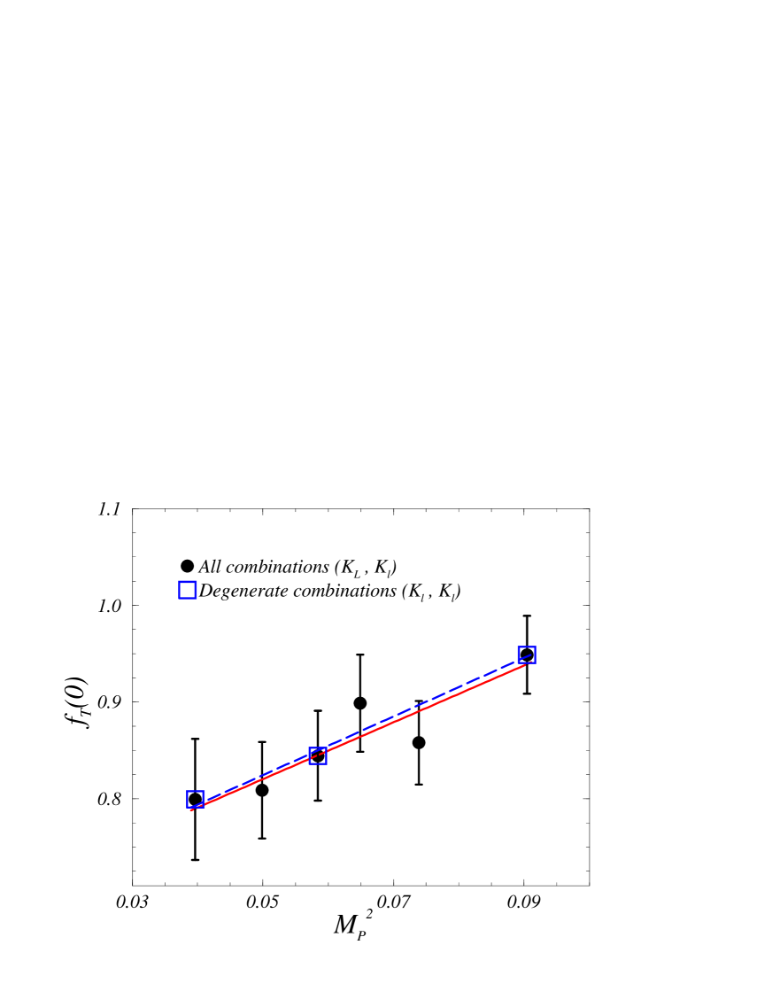
  Figure 2: $f_{T}(0)$ as a function of the squared pseudoscalar meson mass in lattice units. The full (dashed) line represents a fit of the lattice points to eq. (32) for all (degenerate) meson masses.

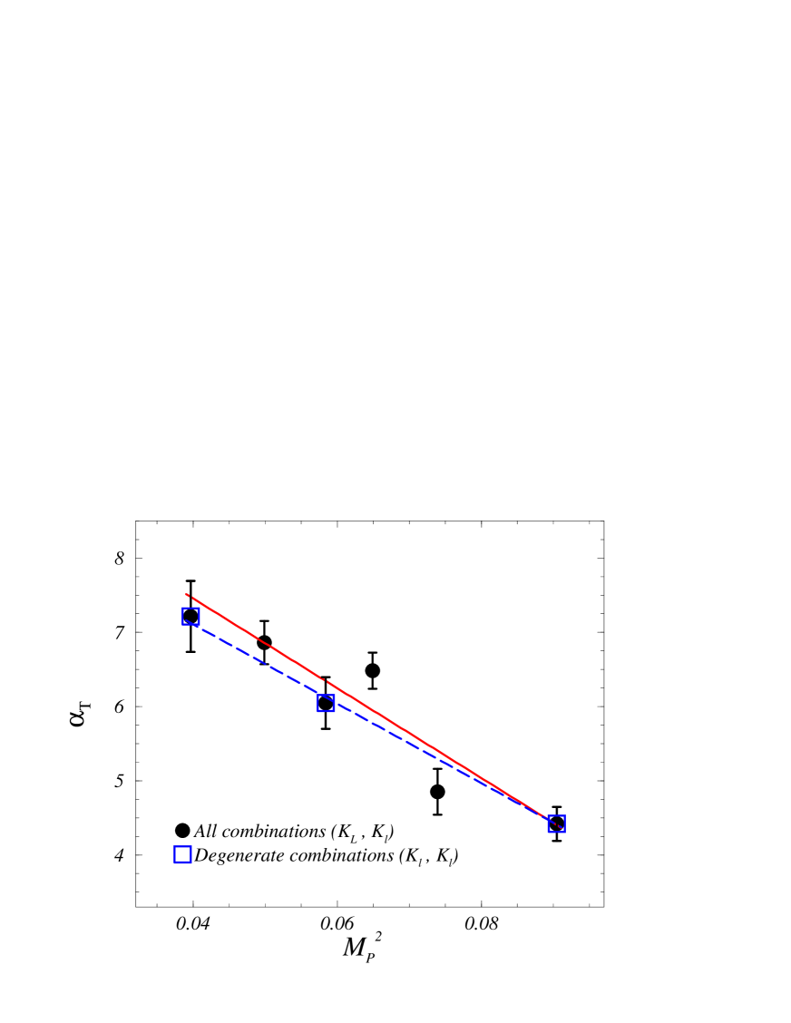
  Figure 3: $\alpha_{T}$ as a function of the squared pseudoscalar meson mass. The curves represent a fit of the lattice points to the eq. (32).

  From figs. 2 and 3, we see that SU(3) breaking effects are small since all the points are rather close to the straight lines of the fit. The two lines correspond either to a fit to all the points or to those corresponding to degenerate mesons ($M_{P}(K_{L},K_{l})=M_{P}(K_{l},K_{l})$) only.

• we have chosen for $f_{T}(0)$ and $\alpha_{T}$ a fitting formula which accounts for SU(3) breaking effects

  $$y=C+\tilde{L}\,M^{2}_{P}(K_{L},K_{l})+L\,M^{2}_{P}(K_{l},K_{l})$$ (34)

  In this case the results read

  $$f_{T}(0) = 0.78(6)\;\;\;C_{f_{T}(0)}=0.67(8)\;\;\;\tilde{L}_{f_{T}(0)}=3.1(7)\;\;\;L_{f_{T}(0)}=-0.14(72)$$

  $$\alpha_{T} = 8.1(4)\;\;\;C_{\alpha_{T}}=9.5(7)\;\;\;\tilde{L}_{\alpha_{T}}=-38(10)\;\;\;L_{\alpha_{T}}=-20(4)$$

  We conclude that SU(3) breaking effects are very small for $f_{T}(0)$ and quite small for $\alpha_{T}$. In the following, for physical applications we will use the results in eq. (LABEL:eq:ftfinal).

Using the physical $K^{0}$ and $\pi$ masses, from eq. (LABEL:eq:ftfinal) we obtain

$$B_{T}=1.23\pm 0.09\,,\quad\quad\lambda_{T}=0.022\pm 0.001\ ,$$ (36)

at a renormalization scale $\mu=2$ GeV. If one needs the operator at another value of $\mu$, the slope will remain the same, whereas $B_{T}$ scales according to the formula [26]

$$B_{T}(\mu_{2}) = \left(\frac{\alpha_{s}(\mu_{2})}{\alpha_{s}(\mu_{1})}\right)^{4/(33-2\,n_{f})}\left[1\ +\ \frac{2}{9}\left({12411-126\,n_{f}+52\,n_{f}^{2}\over(33-2\,n_{f})^{2}}\right){\alpha_{s}(\mu_{2})-\alpha_{s}(\mu_{1})\over 4\pi}\right]B_{T}(\mu_{1})$$ (37)

$$= \left(\frac{\alpha_{s}(\mu_{2})}{\alpha_{s}(\mu_{1})}\right)^{4/33}\left[1\ +\ {1379\over 2178}{\alpha_{s}(\mu_{2})-\alpha_{s}(\mu_{1})\over\pi}\right]B_{T}(\mu_{1})\,,$$

where we set $n_{f}=0$, since we are working in the quenched approximation. In ref. [21] it was shown that even the one-loop evolution gives a very satisfactory description of the scale dependence of the matrix elements of the non-perturbatively renormalized EMO.

We also present our result for the ratio $B_{T}/f^{+}(0)$ extrapolated to the physical point

$$\frac{B_{T}}{f^{+}(0)}=1.18\pm 0.09\ .$$ (38)

This number is lower than the result obtained by combining $B_{T}=1.23\pm 0.09$ and $f^{+}(0)=0.978$, namely $B_{T}/f^{+}(0)=1.26\pm 0.09$. This happens because, on our data, we get $f^{+}(0)=1.04\pm 0.06$ , which is $6\%$ larger than the result of ref. [14]. This is why it is important to have a direct determination of $B_{T}/f^{+}(0)$: systematic effects are expected to be smaller in the ratio. Moreover, the comparison between the two ways to compute $B_{T}/f^{+}(0)$ allows us to evaluate the systematic uncertainty. Indeed the difference between the two way of determining $B_{T}/f^{+}(0)$ is compatible in size with the uncertainty which can be estimated by extrapolating the data using different procedures. In this case, the different extrapolations give results varying by about $5\%$. Thus we take $5\%$ as a measure of a further systematic uncertainty on the determination of the ratio $B_{T}/f^{+}(0)$. From eqs. (36), using $f^{+}(0)=0.978$, and from eq. (38), we obtain $\tilde{B}_{T}=1.25\pm 0.09$ and $\tilde{B}_{T}=1.17\pm 0.09$, respectively. Considering the difference as a systematic error, we end up with our final result, which was given already in eq. (26).

4 Conclusion

We have presented the first lattice calculation of the matrix element $\langle\pi^{0}|Q_{\gamma}^{+}|K^{0}\rangle$. The operator is renormalized non-perturbatively in the RI-MOM scheme which, at the NLO, is equal to the $\overline{MS}$ scheme. Including the statistical and systematic uncertainties (except quenching), our final result has an error smaller than $10\%$. This allows, from the upper limit on ${\rm B}(K_{L}\to\pi^{0}e^{+}e^{-})$, to put more stringent bounds on squark-mass differences in supersymmetric extensions of the Standard Model.

References

-
[1]
A. Alavi-Harati et al. (KTeV Collab.), Phys. Rev. Lett. 83, 22 (1999);
V. Fanti et al. (NA48 Collab.), Phys. Lett. B465, 335 (1999). -
[2]
S. Bertolini, M. Fabbrichesi, J.O. Eeg, hep-ph/9802405;
J. Bijnens and J. Prades, JHEP 01, 023 (1999);
T. Hambye, G.O. Köhler, E.A. Paschos and P.H. Soldan, Nucl. Phys. B564, 391 (2000);
A.A. Bel’kov, G. Bohm, A.V. Lanyov and A.A. Moshkin, hep-ph/9907335;
S. Bosch et al., Nucl. Phys. B565, 3 (2000);
M. Ciuchini et al., Nucl. Phys. B573, 201 (2000). - [3] C. Avilez, Phys. Rev. D23, 1124 (1981)
- [4] G. Isidori, G. Martinelli and G. D’Ambrosio, Phys. Lett. B480, 164 (2000).
- [5] X.-G. He, H. Murayama, S. Pakvasa, G. Valencia, Phys. Rev. D61, 071701 (2000).
- [6] A. Masiero and H. Murayama, Phys. Rev. Lett. 83, 907 (1999);
-
[7]
K.S. Babu, B. Dutta and R. N. Mohapatra,
Phys. Rev. D61, 091701 (2000), hep-ph/9905464;
S. Khalil and T. Kobayashi, Phys. Lett. B460, 341 (1999), hep-ph/9906374;
S. Baek, J.-H. Jang, P. Ko and J.H. Park, Phys. Rev. D62, 117701 (2000), hep-ph/9907572;
M. Brhlik et al., Phys. Rev. Lett. 84, 3041 (2000), hep-ph/9909480. - [8] R. Barbieri, R. Contino and A. Strumia, Nucl. Phys. B578, 153 (2000).
- [9] A.J. Buras et al., Nucl. Phys. B566, 3 (2000).
- [10] KTeV collaboration, A. Alavi-Harati et al., hep-ex/0009030.
- [11] F. Gabbiani, E. Gabrielli, A. Masiero and L. Silvestrini, Nucl. Phys. B477, 321 (1996).
- [12] L.J. Hall, V.A. Kostelecky and S. Raby, Nucl. Phys. B267, 415 (1986).
- [13] Review of Particle Physics, Eur. Phys. J. C15, 1 (2000).
- [14] J. Gasser and H. Leutwyler, Nucl. Phys. B250, 517 (1984).
- [15] Riazuddin, N. Paver and F. Simeoni, Phys. Lett. B316, 397 (1993).
- [16] G. Colangelo, G. Isidori and J. Portoles, Phys. Lett. B470, 134 (1999).
- [17] As. Abada et al., Nucl. Phys. (Proc. Suppl.) 83-84, 268 (2000).
- [18] M. Lüscher, Les Houches Lectures on “Advanced Lattice QCD”, and refs. therein, hep-lat/9802029.
- [19] S. Sint and P. Weisz.Nucl. Phys. (Proc. Suppl.) 63, 856 (1998); S. Capitani et al., Talk given at 2nd Topical Workshop on Deep Inelastic Scattering off Polarized Targets, Zeuthen,Germany, hep-lat/9711007; A. Borelli, R. Frezzotti, E. Gabrielli and C. Pittori, Nucl. Phys. B40, 382 (1993).
- [20] G.P. Lepage and P.B. Mackenzie, Phys. Rev. D48, 2250 (1993).
- [21] D. Becirevic et al., LPTHE-ORSAY-98-33, hep-lat/9809129.
- [22] G. Martinelli, C. Pittori, C. T. Sachrajda, M. Testa and A. Vladikas, Nucl. Phys. B445 (1995) 81.
-
[23]
M. Luscher, S. Sint, R. Sommer, H. Wittig, Nucl. Phys. B491, 344 (1997);
S. Sint, P. Weiz, Nucl. Phys. B502, 251 (1997). - [24] T. Bhattacharya, R. Gupta, W. Lee and S. Sharpe, hep-lat/0009038.
- [25] C.R. Allton, V. Gimenez, L. Giusti and F. Rapuano, Nucl. Phys. B489, 427 (1997).
- [26] J. A. Gracey, Phys. Lett. B488, 175 (2000).