FERMILAB-Conf-00/279-T
SCIPP 00/37
hep–ph/0010338
October 31, 2000
Report of the Tevatron Higgs Working Group
Abstract
Despite the success of the Standard Model (SM), which provides a superb description of a wide range of experimental particle physics data, the dynamics responsible for electroweak symmetry breaking is still unknown. Its elucidation remains one of the primary goals of future high energy physics experimentation. Present day global fits to precision electroweak data based on the Standard Model favor the existence of a weakly-interacting scalar Higgs boson, which is a remnant of elementary scalar dynamics that drives electroweak symmetry breaking. The only known viable theoretical framework incorporating light elementary scalar fields employs “low-energy” supersymmetry, where the scale of supersymmetry breaking is (1 TeV). The Higgs sector of the Minimal Supersymmetric extension of the Standard Model (MSSM) is of particular interest because it predicts the existence of a light CP-even neutral Higgs boson with a mass below about 130 GeV. Moreover, over a significant portion of the MSSM parameter space, the properties of this scalar are indistinguishable from those of the SM Higgs boson.
In Run 2 at the Tevatron, the upgraded CDF and DØ experiments will enjoy greatly enhanced sensitivity in the search for the SM Higgs boson and the Higgs bosons of the MSSM. This report presents the theoretical analysis relevant for Higgs physics at the Tevatron collider and documents the Higgs Working Group simulations to estimate the discovery reach of an upgraded Tevatron for the SM and MSSM Higgs bosons. Based on a simple detector simulation, we have determined the integrated luminosity necessary to discover the SM Higgs in the mass range 100–190 GeV. The first phase of the Run 2 Higgs search, with a total integrated luminosity of 2 fb-1 per detector, will provide a 95% CL exclusion sensitivity comparable to that expected at the end of the LEP2 run. With 10 fb-1 per detector, this exclusion will extend up to Higgs masses of 180 GeV, and a tantalizing effect will be visible if the Higgs mass lies below 125 GeV. With 25 fb-1 of integrated luminosity per detector, evidence for SM Higgs production at the 3 level is possible for Higgs masses up to 180 GeV. However, the discovery reach is much less impressive for achieving a 5 Higgs boson signal. Even with 30 fb-1 per detector, only Higgs bosons with masses up to about 130 GeV can be detected with 5 significance. These results can also be re-interpreted in the MSSM framework and yield the required luminosities to discover at least one Higgs boson of the MSSM Higgs sector. With 5–10 fb-1 of data per detector, it will be possible to exclude at 95% CL nearly the entire MSSM Higgs parameter space, whereas 20–30 fb-1 is required to obtain a 5 Higgs discovery over a significant portion of the parameter space. Moreover, in one interesting region of the MSSM parameter space (at large ), the associated production of a Higgs boson and a pair is significantly enhanced and provides potential for discovering a non-SM-like Higgs boson in Run 2. Further studies related to charged Higgs boson searches and exploiting other search modes of the neutral Higgs bosons are underway and may enhance the above discovery potential.
Contents
toc
I Theoretical Aspects of Higgs Physics at the Tevatron
I.1 Introduction: the Quest for the Origin of Electroweak Symmetry Breaking
With the discovery of the top quark at the Tevatron Tevatron , the Standard Model of particle physics appears close to final experimental verification. Ten years of precision measurements of electroweak observables at LEP, SLC and the Tevatron have failed to find any definitive departures from Standard Model predictions ELW ; Arno ; strom . In some cases, theoretical predictions have been checked with an accuracy of one part in a thousand or better. The consistency of these calculations is evidenced by the excellent agreement between the value of the top quark mass measured directly at the Tevatron, and the corresponding value deduced from precisely measured electroweak observables at LEP and SLC that are sensitive to top-quark loop radiative corrections.
Although the global analysis of electroweak observables provides a superb fit to the Standard Model predictions, there is still no direct experimental evidence for the underlying dynamics responsible for electroweak symmetry breaking. The observed masses of the and bosons can be understood as a consequence of three Goldstone bosons ( and ) that end up as the longitudinal components of the gauge bosons. However, the origin of the Goldstone bosons still demands an explanation. The electroweak symmetry breaking dynamics that is employed by the Standard Model posits a self-interacting complex doublet of scalar fields, which consists of four real degrees of freedom. Renormalizable interactions are arranged in such a way that the neutral component of the scalar doublet acquires a vacuum expectation value, GeV, which sets the scale of electroweak symmetry breaking. Consequently, three massless Goldstone bosons are generated, while the fourth scalar degree of freedom that remains in the physical spectrum is the CP-even neutral Higgs boson of the Standard Model. It is further assumed in the SM that the scalar doublet also couples to fermions through Yukawa interactions. After electroweak symmetry breaking, these interactions are responsible for the generation of quark and charged lepton masses.
The self-interacting scalar field is only one model of electroweak symmetry breaking; other approaches, based on very different dynamics, are also possible. For example, one can introduce new fermions and new dynamics (i.e., new forces), in which the Goldstone bosons are a consequence of the strong binding of the new fermion fields techni . Present experimental data are not sufficient to identify with certainty the nature of the dynamics responsible for electroweak symmetry breaking. The quest to understand electroweak symmetry breaking requires continued experimentation at present and future colliders: the upgraded Tevatron, the LHC and proposed lepton colliders under development.
As described above, the Standard Model is clearly a very good approximation to the physics of elementary particles and their interactions at an energy scale of GeV and below. However, theoretical considerations teach us that the Standard Model is not the ultimate theory of the fundamental particles and their interactions. At an energy scale above the Planck scale, GeV, quantum gravitational effects become significant and the Standard Model must be replaced by a more fundamental theory that incorporates gravity.111Similar conclusions also apply to recently proposed extra-dimensional theories in which quantum gravitational effects can become significant at energies scales as low as (1 TeV) ED . It is also possible that the Standard Model breaks down at some energy scale (called ) below the Planck scale. In this case, the Standard Model degrees of freedom are no longer adequate for describing the theory above and new physics must become relevant. One possible signal of this occurrence lies in the behavior of the Standard Model couplings. The Standard Model is not an asymptotically free theory since some of the couplings (e.g., the U(1) gauge coupling, the Higgs–top-quark Yukawa coupling, and the Higgs self-coupling) eventually blow up at some high energy scale. Among these couplings, only the Higgs self-coupling may blow up at an energy scale below . Of course, there may be other experimental or theoretical hints that new degrees of freedom exist at some high energy scale below . For example, the recent experimental evidence for neutrino masses of order eV or below cannot be strictly explained in the Standard Model. Yet, one can easily write down a dimension-5 operator that is suppressed by , which is responsible for neutrino masses. If eV, then one obtains as a rough estimate GeV.
It is clear from the above discussion that the Standard Model is not a fundamental theory; at best, it is an effective field theory EFT . At an energy scale below , the Standard Model (with higher-dimension operators to parameterize the physics generated at ) provides an extremely good description of all observable phenomena. Therefore, an essential question that future experiments must address is: what is the minimum scale at which new physics beyond the Standard Model must enter? The search for the origin of electroweak symmetry breaking and the quest to identify are intimately tied together. We can consider two scenarios. In the first scenario, electroweak symmetry breaking dynamics results in the existence of a single Higgs boson as posited by the Standard Model. In this case, one would ask whether new phenomena beyond the Standard Model must enter at an energy scale that is accessible to experiment. In the second scenario, electroweak symmetry breaking dynamics does not result in a weakly-coupled Higgs boson as assumed in the Standard Model. In this case, the effective theory that describes current data is a theory that contains the Standard Model fields excluding the Higgs boson. In such an approach, the latter effective field theory must break down at in order to restore the unitarity of the theory, and new physics associated with the electroweak symmetry breaking dynamics must enter.
Although current data provides no direct evidence to distinguish between the two scenarios just described, there is indirect evidence that could be interpreted as favoring the first approach. Namely, the global Standard Model fit to electroweak data takes the Higgs mass as a variable to be fitted. The results of the LEP Electroweak Working Group analysis yields Arno :
| (1) |
In fact, direct searches at LEP show no evidence for the Higgs boson, and imply that GeV LEPHiggs at the 95% CL.222Preliminary results from the 2000 LEP run show no clear evidence of the Higgs boson, with a corresponding Higgs mass lower limit of 113.2 GeV (at 95% CL) LEPHiggsprelim ; tomjunk . Thus, it probably is more useful to quote the 95% CL upper limit that is obtained in the global Standard Model fit Arno : 333The 95% CL upper limit can change by as much as GeV depending on the analysis. More recent upper Higgs mass limits, ranging between 170 GeV and 210 GeV, were presented at the ICHEP 2000 meeting in Osaka, Japan and reviewed in ref. strom .
| (2) |
These results reflect the logarithmic sensitivity to the Higgs mass via the virtual Higgs loop contributions to the various electroweak observables. The Higgs mass range above is consistent with a weakly-coupled Higgs scalar that is expected to emerge from the Standard Model scalar dynamics (although the Standard Model does not predict the mass of the Higgs boson; rather it relates it to the strength of the scalar self-coupling).
Henceforth, we shall take the above result as an indication that the Standard Model (with a weakly-coupled Higgs boson as suggested above) is the appropriate effective field theory at the 100 GeV scale. If this is the case, then the eventual discovery of the Higgs boson will have a profound effect on the determination of , the scale at which the Standard Model must break down. The key parameter for constraining is the Higgs mass, . If is too large, then the Higgs self-coupling blows up at some scale below the Planck scale hambye . If is too small, then the Higgs potential develops a second (global) minimum at a large value of the scalar field of order quiros . Thus new physics must enter at a scale or below in order that the true minimum of the theory correspond to the observed SU(2)U(1) broken vacuum with GeV. Thus, given a value of , one can compute the minimum and maximum Higgs mass allowed. The results of this computation (with shaded bands indicating the theoretical uncertainty of the result) are illustrated in fig. 1.

Three Higgs boson mass ranges are of particular interest:
-
1.
110 GeV 130 GeV
-
2.
130 GeV 180 GeV
-
3.
180 GeV 190 GeV
In mass range 1, the Higgs boson mass lies above the present direct LEP search limit. Moreover, if the Higgs boson were discovered in this range, then fig. 1 would imply that . Finally, as we shall explain in Section I.C, this is the mass range expected in the minimal supersymmetric model. Mass range 2 corresponds to a range of Higgs masses which would be consistent with . In such a scenario, the Standard Model could in principle remain viable all the way up to the Planck scale. Finally, in mass range 3, we are still consistent with the 95% CL Higgs mass limit quoted in eq. (2). Again, a Higgs boson discovered in this mass range would imply that .
I.2 The Standard Model Higgs Boson
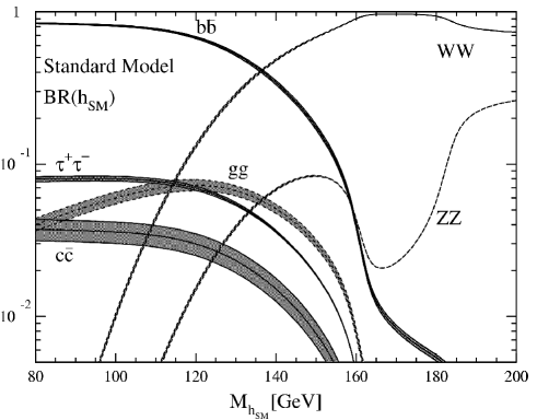
In the Standard Model, the Higgs mass is given by: , where is the Higgs self-coupling parameter. Since is unknown at present, the value of the Standard Model Higgs mass is not predicted. However, other theoretical considerations, discussed in Section I.A, place constraints on the Higgs mass as exhibited in fig. 1. In contrast, the Higgs couplings to fermions and gauge bosons are predicted by the theory. In particular, the Higgs couplings are proportional to the corresponding particle masses, as shown in fig. 2. The vertices of fig. 2 govern the most important features of Higgs phenomenology at colliders. In Higgs production and decay processes, the dominant mechanisms involve the coupling of the Higgs boson to the , and/or the third generation quarks and leptons. It should be noted that a (=gluon) coupling is induced by virtue of a one-loop graph in which the Higgs boson couples to a virtual pair. Likewise, a coupling is generated, although in this case the one-loop graph in which the Higgs boson couples to a virtual pair is the dominant contribution. Further details of Standard Higgs boson properties are given in ref. hhg .


I.2.1 Present Status of the Standard Model Higgs Boson Search
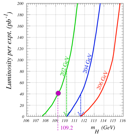
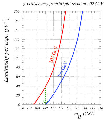
Before turning to the relevant Standard Model Higgs production processes and decay modes at the Tevatron, we briefly comment on the expected status of the Higgs search at the end of the final year of the LEP2 collider run in 2000. In 2000, the LEP2 collider operated at a variety of center-of-mass energies between 203 and 208 GeV (with most data taken at 204.9 GeV and 206.8 GeV). The total integrated luminosity exceeds 100 pb-1 per experiment. If no Higgs signal is seen, then the 95% CL lower limit on the Standard Model Higgs mass is projected to be GeV. In order to discover the Higgs boson at the level, one must have GeV. These results are based on fig. 3 and , taken from ref. egross .
One of the goals of the Higgs Working Group is to examine the potential for the upgraded Tevatron to extend the LEP2 Higgs search. We now briefly survey the dominant Higgs decay and production processes most relevant to the Higgs search at the upgraded Tevatron.
I.2.2 Standard Model Higgs Boson Decay Modes
The branching ratios for the dominant decay modes of a Standard Model Higgs boson are shown as a function of Higgs boson mass in fig. 4 and table 1 9 .
For Higgs boson masses below about 130 GeV, the
decay
dominates, while the decay can also be
phenomenologically relevant.
| [GeV] | |||||||
|---|---|---|---|---|---|---|---|
| 80 | 0.841 | ||||||
| 90 | 0.829 | ||||||
| 100 | 0.811 | ||||||
| 110 | 0.769 | ||||||
| 120 | 0.677 | 0.132 | |||||
| 130 | 0.526 | 0.287 | |||||
| 140 | 0.342 | 0.483 | |||||
| 150 | 0.175 | 0.681 | |||||
| 160 | 0.901 | ||||||
| 170 | 0.965 | ||||||
| 180 | 0.935 | ||||||
| 190 | 0.776 | 0.219 | |||||
| 200 | 0.735 | 0.261 |
These results have been obtained with the program HDECAY hdecay , and include QCD corrections beyond the leading order DSZ .444The leading electroweak corrections are small in the Higgs mass range of interest and may be safely neglected. The QCD corrections are significant for the decay widths due to large logarithmic contributions. The dominant part of these corrections can be absorbed by evaluating the running quark mass at a scale equal to the Higgs mass. In order to gain a consistent prediction of the partial decay widths one has to use masses, [where is the corresponding quark pole mass], obtained by fits to experimental data. The evolution of to is controlled by the renormalization group equations for the running masses. A recent analysis of this type can be found in ref. quarkmasses . For example, for , the following quark masses are obtained: GeV and GeV. Using GeV, it follows that the following hierarchy of Higgs branching ratios is expected for Higgs masses of order 100 GeV: and . Note that the large decrease in the charm quark mass due to QCD running is responsible for suppressing relative to , in spite of the color enhancement of the former, thereby reversing the naively expected hierarchy. In fig. 4, the shaded bands indicate the theoretical uncertainty in the predicted branching ratios. These arise primarily from the uncertainty in , and to a lesser extent the uncertainty in the quark masses.
Though one–loop suppressed, the decay is competitive
with other decays in the relevant Higgs mass region because of the
large top Yukawa
coupling and the color factor. The partial width for this decay is
primarily of interest because it determines the production
cross-section.
For Higgs boson masses above about 110 GeV, the decay mode
, where (at least) one of the bosons is
off-shell (denoted henceforth by ) becomes relevant.
Above 135 GeV, this is the dominant decay mode
13 ; 16 .
The corresponding Higgs branching ratio to is less useful
for the Tevatron Higgs search, while constituting the gold-plated mode
for the Higgs search at the LHC lhchiggs when both bosons
decay to electrons or muons.
I.2.3 Standard Model Higgs Boson Production at the Tevatron
This section describes the most important Higgs production processes at the Tevatron. The relevant cross-sections are depicted in fig. 5 (based on computer programs available from M. Spira hxsec ), and the corresponding numerical results are given in table 2 9 ; DSSW ; private .
Combining these Higgs production mechanisms with the decays discussed in the previous section, one obtains the most promising signatures.

| [GeV] | , | , | |||||
|---|---|---|---|---|---|---|---|
| 80 | 2.132 | 0.616 | 0.334 | 0.163 | |||
| 90 | 1.557 | 0.431 | 0.238 | 0.138 | |||
| 100 | 1.170 | 0.308 | 0.173 | 0.117 | |||
| 110 | 0.900 | 0.224 | 0.128 | 0.100 | |||
| 120 | 0.704 | 0.165 | |||||
| 130 | 0.558 | 0.124 | |||||
| 140 | 0.448 | ||||||
| 150 | 0.364 | ||||||
| 160 | 0.298 | ||||||
| 170 | 0.247 | ||||||
| 180 | 0.205 | ||||||
| 190 | 0.172 | ||||||
| 200 | 0.145 |
[ or ]
Given sufficient luminosity, the most promising
Standard Model Higgs discovery mechanism at the Tevatron for GeV
consists of annihilation into a virtual ( or ),
where the virtual followed by and
the leptonic decay of the Stange:1994ya .
The cross-section for (summed over both
charge states) reaches values of — pb for
GeV as shown in fig. 5,
taken from ref. 9 .
The corresponding cross-section is roughly a
factor of two lower over the same Higgs mass range. The QCD corrections
to coincide with those
of the Drell-Yan process and increase the cross-sections by about 30%
23 ; 23a0 ; 23a . The
theoretical uncertainty is estimated to be about from the
remaining scale dependence. The dependence on different sets of parton
densities is rather weak and also leads to a variation of the
production cross-sections by about 15%.
In order to discover a Higgs signal in at the Tevatron, one must be able to separate the signal from an irreducible Standard Model background. The kinematic properties of the signal and background are not identical, so by applying appropriate cuts, a statistically significant signal can be extracted given sufficient luminosity. Although the Standard Model signal can be studied experimentally, a reliable theoretical computation of the predicted differential cross-section is an essential ingredient of the Tevatron Higgs search.
At lowest order in QCD perturbation theory, the rate for production is of . The appropriate energy scale of the strong coupling constant is not fixed at lowest order, leading to a significant ambiguity in the theoretical predictions. Recently, the QCD next-to-leading order (NLO) corrections to the differential cross-section were calculated kellis . The higher order corrections greatly reduce the scale dependence of the predicted rate. Therefore, we now have a better absolute prediction from theory, and one might be tempted to simply rescale the tree-level cross-section used above to match the NLO result for the overall rate. However, the NLO calculation may also change the shape of kinematic distributions from the lowest order results. In particular, the NLO calculation determines more accurately the kinematics of the pair, and thus permits an extrapolation of the distribution to higher values than have been measured. Unfortunately, the NLO cross-sections are generally not reliable for describing details of the kinematic distributions, since these are sensitive to the details of the hadronization and fragmentation of the final state. In order to overcome this deficiency, a consistent treatment that combines the NLO calculations with the Monte Carlo simulations is required. The analyses presented in Section II of this report have not yet taken advantage of the new information provided by the NLO result.
The signatures of Higgs production in the channel are governed by the corresponding decays of the Higgs and vector boson. The dominant decay mode of the Higgs boson in the mass range of GeV is ; in this case, the leptonic decays of the final state and (these include the missing energy signature associated with ) serve as a trigger for the events and significantly reduce QCD backgrounds. The detection of the Higgs signal via the more copious four-jet final states resulting from hadronic decays of the and is severely hampered by huge irreducible backgrounds.
For GeV, the Higgs decay mode (where one is off-shell if ) becomes dominant. In this case, the final state consists of three gauge bosons, ( or ), and the like-sign di-lepton signature becomes the primary signature for Higgs discovery.
The gluon fusion processes proceeds primarily through
a top quark triangle loop 29a ; sally ; 19 , and
is the dominant neutral Higgs
production mechanism at the Tevatron, with cross-sections
of roughly — pb for
GeV,
as shown in fig. 5.
The two-loop QCD corrections enhance the gluon fusion cross-section by
about 60—100% 19 . These are dominated by
soft and collinear gluon radiation in the Standard Model 29 .555Multiple soft-gluon emission also has a large effect
on the Higgs boson transverse momentum distribution balazs .
The remaining scale dependence results in a theoretical
uncertainty of about . The dependence of the gluon fusion
cross-section on different parton densities yields roughly an additional
15% uncertainty in the theoretical prediction.
The analytical QCD corrections to Higgs boson plus one jet production
have recently
been evaluated in the limit of heavy top quarks, but there is no
numerical analysis so far 30 .
The signature is not promising at the Tevatron due to the overwhelming QCD background of production. The signature, although not thoroughly studied, probably requires a missing resolution beyond the capabilities of the upgraded CDF and DØ detectors. For GeV, the decay channel becomes dominant and provides a potential Higgs discovery mode for the Tevatron. The strong angular correlations of the final state leptons resulting from is one of the crucial ingredients for this discovery channel 5 ; dreiner .
[ or ]
Vector boson fusion is a shorthand notation for the full
process, where the quark and anti-quark both radiate
virtual vector bosons ()
which then annihilate to produce the Higgs boson. Vector
boson fusion via (and its charge-conjugate process)
is also possible, although the
relative contribution is small at the Tevatron. In fig. 5,
all contributing
processes are included, labeled for simplicity.
The resulting Standard Model cross-sections are in the range — pb for
GeV.
The QCD corrections enhance the cross-section by about 10% 23a ; 32 .
The modest fusion cross-section precludes observation of any of the rare SM Higgs decay modes in events at the Tevatron. For example, for GeV and 30 fb-1 of data, only six events are expected from the production process . Similarly, under the same assumptions, only eleven di-lepton events resulting from are expected from the same data sample prior to any acceptance cuts that are required to reduce the large , or backgrounds. Typically these cuts reduce the Higgs signal by another order of magnitude or more wbfLHC .
For GeV, the dominant Higgs decay channel is . In events, the Higgs boson would appear as a invariant mass peak in 4-jet events in which two of the jets are identified as -quarks. Note that the final state can also arise from and events. These channels are very difficult to detect due to the very large QCD backgrounds. In the case of fusion, because there are two forward jets in the full process , one may hope to be able to somewhat suppress the QCD backgrounds by appropriate cuts. A preliminary analysis is presented in Section II.B.4c. The initial conclusion is that this channel does not appear to be promising at the upgraded Tevatron.
,
The theoretical predictions for the cross-section of associated
production of a Higgs boson and a heavy quark pair,
, ()666At Tevatron energies,
the annihilation contribution
dominates over -fusion for production, whereas
the reverse is true for production.
Both mechanisms are included in the results exhibited in fig. 5 and in table 2. are shown in fig. 5 and in table 2.
The tree-level cross-section for , is displayed in fig. 5 and in table 2. Although the full NLO QCD result is not presently known, the NLO QCD corrections are known in the limit of 24 . In this limit the cross-section factorizes into the production of a pair, which is convolved with a splitting function for Higgs radiation , resulting in an increase of the cross-section by about 20–60%. However, since this equivalent Higgs approximation is only valid to within a factor of two, this result may not be sufficiently reliable.
The case of associated production of a Higgs boson and a bottom quark pair () is more subtle and requires a separate discussion. For values of (which is satisfied in practice), the total inclusive cross-section is known at next-to-leading order DSSW . The leading-order process is , where the initial quarks reside in the proton sea. Since the quark sea arises from the splitting of gluons into pairs, the final state is actually , but the final state quarks tend to reside at low transverse momentum. The next-to-leading-order correction to this process is modest, indicating that the perturbative expansion is under control. Large logarithms, , which arise in the calculation are absorbed into the distribution functions. The calculation also makes evident that the Yukawa coupling of the Higgs to the bottom quarks should be evaluated from the running mass evaluated at the Higgs mass scale, [as in the case of the QCD-corrected decay rate for ], rather than the running mass evaluated at the quark mass or the physical (“pole”) mass.
The relation between the cross-section and the cross-section requires some clarification. For example, it is not correct to simply add the results of the cross-section and the cross-section for associated production, since logarithmic terms [proportional to ] in the latter have been incorporated into the -quark distribution functions that appear in the former. However, one can subtract out these logarithmic terms. The resulting subtracted cross-section (which can be negative) can be added to the previously obtained cross-section without double counting soper ; 25 . Likewise, the processes and also contribute and the relevant logarithms must be subtracted before adding the corresponding cross-sections 25 . Nevertheless, we have checked that for the correction due to the subtracted cross-section is small DSSW ; private . Thus, the NLO QCD-corrected cross-section should provide a fairly reliable estimate to the total inclusive cross-section.777For a completely consistent computation, one would need to include two-loop (NNLO) QCD corrections to and the one-loop (NLO) QCD corrections to (and its charge-conjugate process). [Note that for , the -quark parton distribution function is of order .] The modest size of the NLO corrections to suggest that the corrections are probably small.
In practice, the total inclusive cross-section for Higgs production in association with a bottom quark pair is not measurable at the Tevatron, since one must observe one or both of the final-state quarks in order to isolate the signal above other Standard Model backgrounds. Hence one or both of the final state quarks must be produced at large transverse momentum. This is a fraction of the total inclusive cross-section, depending on the minimum transverse momentum required on one or both quarks. The leading-order process for Higgs production in association with a pair of high transverse momentum quarks is . Since this process is known only at leading order, the theoretical uncertainty in the cross-section is large. Clearly, it is very important to compute the NLO QCD corrections for the differential cross-section (as a function of the final state quark transverse momenta) for production. This computation is not yet available in the literature.
The tree-level , cross-section (as a function of ) shown in fig. 5 has been computed by fixing the scales of the initial (CTEQ4M CTEQ ) parton densities, the running coupling and the running Higgs–bottom-quark Yukawa coupling (or equivalently, the running -quark mass) at the value of the corresponding mass. In particular, by employing the running quark mass evaluated at , we are implicitly resumming large logarithms associated with the QCD-corrected Yukawa coupling. Thus, the tree-level cross-section displayed in fig. 5 implicitly includes a part of the QCD corrections to the full inclusive cross-section.888The effect of using the running -quark mass [] as opposed to the -quark pole mass [ GeV] is to reduce the cross-section by roughly a factor of two. Nevertheless, as emphasized above, the most significant effect of the QCD corrections to production arises from the kinematical region where the quarks are emitted near the forward direction. In fact, large logarithms arising in this region spoils the convergence of the QCD perturbation series since . These large logarithms (already present at lowest order) must be resummed to all orders, and this resummation is accomplished by the generation of the -quark distribution function as described above. Thus, the QCD-corrected fully inclusive cross-section is well approximated by and its QCD corrections. The latter is also exhibited in fig. 5 and is seen to be roughly an order of magnitude larger than the tree-level cross-section. Of course, this result is not very relevant for the Tevatron experimental searches in which transverse momentum cuts on the -jets are employed. Ultimately, one needs the QCD-corrected differential cross-section for (as a function of the final state -quark transverse momenta) in order to do realistic simulations of the Higgs signal in this channel.
Based on our best estimates for the production cross-sections shown in fig. 5, we conclude that in the Standard Model both processes of Higgs radiation off top and bottom quarks have very small event rates. However, in some extensions of the Standard Model, the coupling of the Higgs boson to can be significantly enhanced. This leads to enhanced production which may be observable at an upgraded Tevatron with sufficient luminosity. A concrete example (the minimal supersymmetric model at large ) will be discussed further in Section I.C.6a.
To detect enhanced production, we assume that the dominant decay of the Higgs boson is into pairs. Thus, the signal must be extracted from events with four -quarks (suggesting the need for tagging at least three of the -jets). Theoretical estimates of the Standard Model background rates are less reliable than the corresponding rates discussed above. Heavy quark production rates are typically difficult to estimate, and the situation is complicated by demanding 3 or 4 –tagged jets. Improved theoretical modeling and detailed comparisons with Run 2 Tevatron data will be essential to improve the present background estimates.
I.3 Higgs Bosons in Low-Energy Supersymmetry
Although the Higgs mass range 130 GeV GeV appears to permit an effective Standard Model that survives all the way to the Planck scale, most theorists consider such a possibility unlikely. This conclusion is based on the “naturalness” natural argument as follows. In an effective field theory, all parameters of the low-energy theory (i.e. masses and couplings) are calculable in terms of parameters of a more fundamental, renormalizable theory that describes physics at the energy scale . All low-energy couplings and fermion masses are logarithmically sensitive to . In contrast, scalar squared-masses are quadratically sensitive to . Thus, in this framework, the observed Higgs mass (at one-loop) has the following form:
| (3) |
where is a parameter of the fundamental theory and is a constant, presumably of , which is calculable within the low-energy effective theory. The “natural” value for the scalar squared-mass is . Thus, the expectation for is
| (4) |
If is significantly larger than 1 TeV (often called the hierarchy problem in the literature), then the only way to find a Higgs mass associated with the scale of electroweak symmetry breaking is to have an “unnatural” cancellation between the two terms of eq. (3). This seems highly unlikely given that the two terms of eq. (3) have completely different origins. As a cautionary note, what appears to be unnatural today might be shown in the future to be a natural consequence of dynamics or symmetry at the Planck scale. Only further experimentation that tests our present understanding can determine if the quest for new physics at scales is ultimately fruitful.
A viable theoretical framework that incorporates weakly-coupled Higgs bosons and satisfies the constraint of eq. (4) is that of “low-energy” or “weak-scale” supersymmetry Nilles85 ; Haber85 ; smartin . In this framework, supersymmetry is used to relate fermion and boson masses (and interactions). Since fermion masses are only logarithmically sensitive to , boson masses will exhibit the same logarithmic sensitivity if supersymmetry is exact. Since no supersymmetric partners of Standard Model particles have been found, we know that supersymmetry cannot be an exact symmetry of nature. Thus, we identify with the supersymmetry-breaking scale. The naturalness constraint of eq. (4) is still relevant, so in the framework of low-energy supersymmetry, the scale of supersymmetry breaking should not be much larger than about 1 TeV in order that the naturalness of scalar masses be preserved. The supersymmetric extension of the Standard Model would then replace the Standard Model as the effective field theory of the TeV scale. One could then ask: at what scale does this model break down? The advantage of the supersymmetric approach is that the effective low-energy supersymmetric theory can be valid all the way up to the Planck scale, while still being natural!
In order to begin our study of Higgs bosons in low-energy supersymmetry, we need a specific model framework. The simplest realistic model of low-energy supersymmetry is a minimal supersymmetric extension of the Standard Model (MSSM), which employs the minimal supersymmetric particle spectrum habermssm . Higgs phenomenology in the MSSM and the corresponding discovery reach at the Tevatron was a primary focus of the Higgs Working Group. Non-minimal supersymmetric approaches are also of interest and have been addressed in part by the Beyond the MSSM Working Group of this workshop btmssm .
I.3.1 The Tree-Level Higgs Sector of the MSSM
Both hypercharge and Higgs doublets are required in any Higgs sector of an anomaly-free supersymmetric extension of the Standard Model. The supersymmetric structure of the theory also requires (at least) two Higgs doublets to generate mass for both “up”-type and “down”-type quarks (and charged leptons) Inoue82 ; Gunion86 . Thus, the MSSM contains the particle spectrum of a two-Higgs-doublet extension of the Standard Model and the corresponding supersymmetric partners Haber85 ; smartin .
The two-doublet Higgs sector hhgchap4 contains eight scalar degrees of freedom: one complex doublet, and one complex doublet, . The notation reflects the form of the MSSM Higgs sector coupling to fermions: [] couples exclusively to down-type [up-type] fermion pairs. When the Higgs potential is minimized, the neutral components of the Higgs fields acquire vacuum expectation values:999The phases of the Higgs fields can be chosen such that the vacuum expectation values are real and positive. That is, the tree-level MSSM Higgs sector conserves CP, which implies that the neutral Higgs mass eigenstates possess definite CP quantum numbers.
| (5) |
where the normalization has been chosen such that . Spontaneous electroweak symmetry breaking results in three Goldstone bosons, which are absorbed and become the longitudinal components of the and . The remaining five physical Higgs particles consist of a charged Higgs pair
| (6) |
one CP-odd scalar
| (7) |
and two CP-even scalars:
(with ). The angle arises when the CP-even Higgs squared-mass matrix (in the — basis) is diagonalized to obtain the physical CP-even Higgs states (explicit formulae will be given below).
The supersymmetric structure of the theory imposes constraints on the Higgs sector of the model. For example, the Higgs self-interactions are not independent parameters; they can be expressed in terms of the electroweak gauge coupling constants. As a result, all Higgs sector parameters at tree-level are determined by two free parameters: the ratio of the two neutral Higgs field vacuum expectation values,
| (8) |
and one Higgs mass, conveniently chosen to be . In particular,
| (9) |
and the CP-even Higgs bosons and are eigenstates of the following squared-mass matrix
| (10) |
The eigenvalues of are the squared-masses of the two CP-even Higgs scalars
| (11) |
and is the angle that diagonalizes the CP-even Higgs squared-mass matrix. From the above results, one obtains:
| (12) |
In the convention where is positive (i.e., ), the angle lies in the range .
An important consequence of eq. (11) is that there is an upper bound to the mass of the light CP-even Higgs boson, . One finds that:
| (13) |
This is in marked contrast to the Standard Model, in which the theory does not constrain the value of at tree-level. The origin of this difference is easy to ascertain. In the Standard Model, is proportional to the Higgs self-coupling , which is a free parameter. On the other hand, all Higgs self-coupling parameters of the MSSM are related to the squares of the electroweak gauge couplings.
Note that the Higgs mass inequality [eq. (13)] is saturated in the limit of large . In the limit of , the expressions for the Higgs masses and mixing angle simplify and one finds
Two consequences are immediately apparent. First, , up to corrections of . Second, up to corrections of . This limit is known as the decoupling limit decoupling because when is large, one can focus on an effective low-energy theory below the scale of in which the effective Higgs sector consists only of one CP-even Higgs boson, . As we shall demonstrate below, the tree-level couplings of are precisely those of the Standard Model Higgs boson when . From eq. (I.3.1), one can also derive:
| (14) |
This result will prove useful in evaluating the CP-even Higgs boson couplings to fermion pairs in the decoupling limit.
The phenomenology of the Higgs sector depends in detail on the various couplings of the Higgs bosons to gauge bosons, Higgs bosons and fermions. The couplings of the two CP-even Higgs bosons to and pairs are given in terms of the angles and by
where
| (15) |
There are no tree-level couplings of or to . Next, consider the couplings of one gauge boson to two neutral Higgs bosons:
From the expressions above, we see that the following sum rules must hold separately for and :
Similar considerations also hold for the coupling of and to . We can summarize the above results by noting that the coupling of and to vector boson pairs or vector–scalar boson final states is proportional to either or as indicated below hhg :
| (16) |
Note in particular that all vertices in the theory that contain at least one vector boson and exactly one non-minimal Higgs boson state (, or ) are proportional to . This can be understood as a consequence of unitarity sum rules which must be satisfied by the tree-level amplitudes of the theory cornwall ; wudka .
In the MSSM, the Higgs tree-level couplings to fermions obey the following property: couples exclusively to down-type fermion pairs and couples exclusively to up-type fermion pairs. This pattern of Higgs-fermion couplings defines the Type-II two-Higgs-doublet model wise ; hhg . The gauge-invariant Type-II Yukawa interactions (using 3rd family notation) are given by:
| (17) |
where is the left-handed projection operator. [Note that (, where .] Fermion masses are generated when the neutral Higgs components acquire vacuum expectation values. Inserting eq. (5) into eq. (17) yields a relation between the quark masses and the Yukawa couplings:
| (18) |
Similarly, one can define the Yukawa coupling of the Higgs boson to -leptons (the latter is a down-type fermion). The couplings of the physical Higgs bosons to the third generation fermions is obtained from eq. (17) by using eqs. (6)–(I.3.1). In particular, the couplings of the neutral Higgs bosons to relative to the Standard Model value, , are given by
(the indicates a pseudoscalar coupling), and the charged Higgs boson couplings to fermion pairs (with all particles pointing into the vertex) are given by
We next consider the behavior of the Higgs couplings at large . This limit is of particular interest since at large , some of the Higgs couplings to down-type fermions can be significantly enhanced.101010In models of low-energy supersymmetry, there is some theoretical prejudice that suggests that , with the fermion running masses evaluated at the electroweak scale. For example, [] is disfavored since in this case, the Higgs–top-quark [Higgs–bottom-quark] Yukawa coupling blows up at an energy scale significantly below the Planck scale. Let us examine two particular large regions of interest. (i) If , then the decoupling limit is reached, in which and . From eqs. (I.3.1)–(I.3.1), it follows that the and couplings have equal strength and are significantly enhanced (by a factor of ) relative to the coupling, whereas the coupling is negligibly small. In contrast, the values of the and couplings are equal to the corresponding couplings of the Standard Model Higgs boson. To show that the value of the coupling [see eq. (I.3.1)] reduces to that of in the decoupling limit, note that eq. (I.3.1) implies that when even when . (ii) If and , then [see fig. 6] and . In this case, the and couplings have equal strength and are significantly enhanced (by a factor of ) relative to the coupling, while the coupling is negligibly small. Using eq. (I.3.1) it follows that the coupling is equal in strength to the coupling. However, the value of the coupling can differ from the corresponding coupling when [since in case (ii), where , the product need not be particularly small]. Note that in both cases above, only two of the three neutral Higgs bosons have enhanced couplings to .


The decoupling limit of is effective for all values of . It is easy to check that the pattern of all Higgs couplings displayed in eqs. (I.3.1)–(I.3.1) respects the decoupling limit. That is, in the limit where , , which means that the couplings to Standard Model particles approach values corresponding precisely to the couplings of the Standard Model Higgs boson. The region of MSSM Higgs sector parameter space in which the decoupling limit applies is large, because approaches one quite rapidly once is larger than about 200 GeV, as shown in fig. 6. As a result, over a significant region of the MSSM parameter space, the search for the lightest CP-even Higgs boson of the MSSM is equivalent to the search for the Standard Model Higgs boson. This result is more general; in many theories of non-minimal Higgs sectors, there is a significant portion of the parameter space that approximates the decoupling limit. Consequently, simulations of the Standard Model Higgs signal are also relevant for exploring the more general Higgs sector.
I.3.2 The Radiatively-Corrected MSSM Higgs Sector: (a) Higgs masses
So far, the discussion has been based on a tree-level analysis of the Higgs sector. However, radiative corrections can have a significant impact on the predicted values of Higgs masses and couplings. The radiative corrections involve both loops of Standard Model particles and loops of supersymmetric partners. The dominant effects arise from loops involving the third generation quarks and squarks and are proportional to the corresponding Yukawa couplings. Thus, we first review the parameters that control the masses and mixing of the third-generation squarks. (We shall neglect intergenerational mixing effects, which have little impact on the discussion that follows.)
For each left-handed and right-handed quark of fixed flavor, , there is a corresponding supersymmetric partner and , respectively. These are the so-called interaction eigenstates, which mix according to the squark squared-mass matrix. The mixing angle that diagonalizes the squark mass matrix will be denoted by . The squark mass eigenstates, denoted by and , are obtained by diagonalizing the following matrix
| (21) |
where and . In addition, , , and for the top-squark (or stop) mass matrix, while , , and for the bottom-squark (or sbottom) mass matrix. The squark mixing parameters are given by
Thus, the top-squark and bottom-squark masses and mixing angles depend on the supersymmetric Higgs mass parameter and the soft-supersymmetry-breaking parameters: , , , and .111111For simplicity, we shall take , and to be real parameters. That is, we are neglecting possible CP-violating effects that can enter the MSSM Higgs sector via radiative corrections. For a discussion of the implications of such effects, see refs. cpcarlos and cpcarlos2 .
The radiative corrections to the Higgs squared-masses have been computed by a number of techniques, and using a variety of approximations such as the effective potential at one-loop early-veff ; veff ; berz ; erz and two-loops zhang ; espizhang ; EZ2 [only the and two-loop results are known], and diagrammatic methods turski ; hhprl ; brig ; madiaz ; 1-loop ; completeoneloop ; hempfhoang ; weiglein . Complete one-loop diagrammatic computations of the MSSM Higgs masses have been presented by a number of groups completeoneloop ; the resulting expressions are quite complex, and depend on all the parameters of the MSSM. Partial two-loop diagrammatic results are also known hempfhoang ; weiglein . These include the contributions to the neutral CP-even Higgs boson squared-masses in the on-shell scheme weiglein .
One of the most striking effects of the radiative corrections to the MSSM Higgs sector is the modification of the upper bound of the light CP-even Higgs mass, as first noted in refs. early-veff and hhprl . Consider the region of parameter space where is large and . In this limit, the tree-level prediction for corresponds to its theoretical upper bound, . Including radiative corrections, the theoretical upper bound is increased. The dominant effect arises from an incomplete cancellation of the top-quark and top-squark loops (these effects actually cancel in the exact supersymmetric limit).121212In certain regions of parameter space (corresponding to large and large values of ), the incomplete cancellation of the bottom-quark and bottom-squark loops can be as important as the corresponding top sector contributions. For simplicity, we ignore this contribution in eq. (23) below. The qualitative behavior of the radiative corrections can be most easily seen in the large top squark mass limit, where in addition, the splitting of the two diagonal entries and the off-diagonal entry of the top-squark squared-mass matrix are both small in comparison to the average of the two stop squared-masses:
| (22) |
In this case, the upper bound on the lightest CP-even Higgs mass is approximately given by
| (23) |
where .
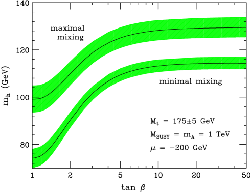
The more complete treatments of the radiative corrections cited above show that eq. (23) somewhat overestimates the true upper bound of . Nevertheless, eq. (23) correctly reflects some noteworthy features of the more precise result. First, the increase of the light CP-even Higgs mass bound beyond can be significant. This is a consequence of the enhancement of the one-loop radiative correction. Second, the dependence of the light Higgs mass on the stop mixing parameter implies that (for a given value of ) the upper bound of the light Higgs mass initially increases with and reaches its maximal value . This point is referred to as the maximal mixing case (whereas corresponds to the minimal mixing case). In a more complete computation that includes both two-loop logarithmic and non-logarithmic corrections, the values corresponding to maximal and minimal mixing are shifted and exhibit an asymmetry under as shown in fig. 7. In the numerical analysis presented in this and subsequent figures in this section, we assume for simplicity that the third generation diagonal soft-supersymmetry-breaking squark squared-masses are degenerate: , which defines the parameter .131313We also assume that , in which case it follows that up to corrections of .

Third, note the logarithmic sensitivity to the top-squark masses. Naturalness arguments that underlie low-energy supersymmetry imply that the supersymmetric particles masses should not be larger than a few TeV. Still, the precise upper bound on the light Higgs mass depends on the specific choice for the upper limit of the stop masses. The dependence of the light Higgs mass obtained by the more complete computation (to be discussed further below) as a function of is shown in fig. 8.


As noted above, the largest contribution to the one-loop radiative corrections is enhanced by a factor of and grows logarithmically with the top squark mass. Thus, higher order radiative corrections can be non-negligible for large top squark masses, in which case the large logarithms must be resummed. The renormalization group (RG) techniques for resumming the leading logarithms have been developed by a number of authors rge ; 2loopquiros ; llog ; carena . The computation of the RG-improved one-loop corrections requires numerical integration of a coupled set of RG equations llog . Although this procedure has been carried out in the literature, the analysis is unwieldy and not easily amenable to large-scale Monte-Carlo studies. It turns out that over most of the parameter range, it is sufficient to include the leading and sub-leading logarithms at two-loop order. (Some additional non-logarithmic terms, which cannot be ascertained by the renormalization group method, must also be included chhhww .) Compact analytic expressions have been obtained for the dominant one and two-loop contributions to the matrix elements of the radiatively-corrected CP-even Higgs squared-mass matrix:
| (24) |
where the tree-level contribution was given in eq. (10) and is the contribution from the radiative corrections. Diagonalizing this matrix yields radiatively-corrected values for , and the CP-even Higgs mixing angle . Explicit expressions for the , given in refs. carena and hhh , include the dominant leading and sub-leading logarithms at two-loop order (the latter are generated by an iterative solution to the RG-equations). Also included are the leading effects at one loop of the supersymmetric thresholds and the corresponding two-loop logarithmically enhanced terms, which can again be determined by iteration of the RG-equations. The most important effects of this type are squark mixing effects in the third generation. The procedures described above produce a prediction for the Higgs mass in terms of running parameters in the scheme. It is a simple matter to relate these parameters to the corresponding on-shell parameters used in the diagrammatic calculations espizhang ; chhhww .
Additional non-logarithmic two-loop contributions, which can generate a non-negligible shift in the Higgs mass (of a few GeV), must also be included.141414An improved procedure for computing the radiatively-corrected neutral Higgs mass matrix and the charged Higgs mass in a self-consistent way (including possible CP-violating effects), which incorporates one-loop supersymmetric threshold corrections to the Higgs–top-quark and Higgs–bottom-quark Yukawa couplings, can be found in ref. cpcarlos2 . A compact analytical expression that incorporates these effects at was given in ref. compact . An important source of such contributions are the one-loop supersymmetric threshold corrections to the relation between the Higgs–top-quark and Higgs–bottom-quark Yukawa couplings and the corresponding quark masses [see, e.g., eq. (29)]. These generate a non-logarithmic two-loop shift of the radiatively corrected Higgs mass proportional to the corresponding squark mixing parameters. One consequence of these contributions chhhww is the asymmetry in the predicted value of under as noted in fig. 7. Recently, the computation of has been further refined by the inclusion of genuine two-loop corrections of EZ2 . These non-logarithmic corrections, which depend on the stop mixing parameters, can slightly increase the Higgs mass. This improvement is not yet implemented in the figures shown in this section.
The numerical results displayed in figs. 6–10 are based on the calculations of refs. carena and hhh , with improvements as described in refs. weiglein and chhhww . The supersymmetric parameters in the maximal and minimal mixing cases have been chosen according to the first two benchmark scenarios of ref. benchmark (displayed in table 53 of Section III.B.2). Of particular interest is the upper bound for the lightest CP-even Higgs mass (). At fixed , the maximal value of is reached for (see fig. 10). Taking large, fig. 9 illustrates that the maximal value of the lightest CP-even Higgs mass bound is realized at large in the case of maximal mixing. For each value of , we denote the maximum value of by [this value also depends on the third-generation squark mixing parameters]. Allowing for the uncertainty in the measured value of and the uncertainty inherent in the theoretical analysis, one finds for TeV that , where
In practice, parameters leading to maximal mixing are not expected in typical models of supersymmetry breaking. Thus, in general, the upper bound on the lightest Higgs boson mass is expected to be somewhere between the two extreme limits quoted above. Cross-checks among various programs cwprog ; hehprog ; feynhiggs and rough estimates of higher order corrections not yet computed suggest that the results for Higgs masses should be accurate to within about 2 to 3 GeV over the parameter ranges displayed in figs. 7—10.
In fig. 10, we exhibit the masses of the CP-even neutral and the charged Higgs masses as a function of . The squared-masses of the lighter and heavier neutral CP-even Higgs are related by
| (25) |
Note that for all values of and [where is to be evaluated depending on the top-squark mixing, as indicated in eq. (I.3.2)]. It is interesting to consider the behavior of the CP-even Higgs masses in the large regime. For large values of and for , the off-diagonal elements of the Higgs squared-mass matrix become small compared to the diagonal elements ; . Hence the two CP-even Higgs squared-masses are approximately given by the diagonal elements of . As before, we employ the notation where refers to the asymptotic value of at large and (the actual numerical value of depends primarily on the assumed values of the third generation squark mass and mixing parameters). If , then and , whereas if , then and . This behavior can be seen in fig. 10.

I.3.3 The Radiatively-Corrected MSSM Higgs Sector: (b) Higgs couplings
Radiative corrections also significantly modify the tree-level values of the Higgs boson couplings to fermion pairs and to vector boson pairs. As discussed above, the tree-level Higgs couplings depend crucially on the value of . In first approximation, when radiative corrections of the Higgs squared-mass matrix are computed, the diagonalizing angle is renormalized. Thus, one may compute a radiatively-corrected value for . This provides one important source of the radiative corrections of the Higgs couplings. In fig. 6, we show the effect of radiative corrections on the value of as a function of for different values of the squark mixing parameters and . One can then simply insert the radiatively corrected value of into eqs. (I.3.1), (I.3.1) and (I.3.1) to obtain radiatively-improved couplings of Higgs bosons to vector bosons and to fermions.
To better understand the behavior of the Higgs boson couplings to fermion pairs, consider the radiatively corrected CP-even Higgs squared-mass matrix [eq. (24)]. The complete expressions for the individual matrix elements (even after a series of approximations in which many sub-leading terms are dropped) are quite involved, and we will not display them here. However, it is useful to examine the leading contributions to the off-diagonal element, . After including the dominant one–loop corrections induced by the top-squark sector151515If is large, bottom-squark sector effects may become important. For simplicity, these effects will be neglected in the formulae exhibited in this section., together with the two–loop, leading–logarithm effects161616This result is only valid if the splitting between the two top-squark squared-masses is small compared to . In addition, the conditions , must also be fulfilled. CMW1 ; CMW2 ,
where , , is the QCD coupling constant and is the Higgs–top-quark Yukawa coupling [eq. (18)]. The mixing angle can be determined by diagonalizing the CP-even Higgs squared-mass matrix [eq. (24)]:
| (26) |
It follows that in the limit where , either (if ) or (if ). As a result, some of the Higgs boson couplings to quark and lepton pairs [eq. (I.3.1)] can be strongly suppressed, if radiative corrections suppress the value of .171717Although is negative at tree level (implying that ), it is possible that radiative corrections flip the sign of [see eq. (I.3.3)]. Thus, the range of the radiatively corrected angle can be taken to be .
If and is large (values of are sufficient), the resulting pattern of Higgs couplings is easy to understand. In this limit, and , as noted at the end of section I.C.2. Two cases must be treated separately depending on the value of . First, if , then (assuming as in tree-level), and . In this case, the lighter CP-even Higgs boson is roughly aligned along the direction and the heavier CP-even Higgs boson is roughly aligned along the direction [see eq. (I.3.1)]. In particular, the coupling of to and is significantly diminished (since down-type fermions couple to ), while the couplings [eq. (I.3.1)] are approximately equal to those of the Standard Model [since ]. Consequently, the branching ratios of into , , , and can be greatly enhanced over Standard Model expectations CMW1 ; CMW2 ; Wells ; bdhty . Second, if then and and the previous considerations for apply now to .
For moderate or large values of , the vanishing of leads to the approximate numerical relation CMW1 :
| (27) |
where we have replaced , and the weak gauge couplings by their approximate numerical values at the weak scale. For low values of , or large values of the mixing parameters, a cancellation can easily take place for large values of . For instance, if TeV, , and GeV, a cancellation can take place for , with GeV. The heaviest CP–even Higgs boson has Standard Model–like couplings to the gauge bosons [], but the branching ratios for decays into bosons, gluons and charm quarks are enhanced with respect to the SM case: , and .
Although it is difficult to have exact cancellation of the off-diagonal element , in many regions of the supersymmetric parameter space, important suppressions may be present. Generically, the –dependent radiative corrections to depend strongly on the sign of the product ( for large and moderate ) and on the value of . For the same value of , a change in the sign of can lead to observable variations in the branching ratio for the Higgs boson decay into bottom quarks. If , the absolute value of the off–diagonal matrix element, and hence, the coupling of bottom quarks to the Standard Model–like Higgs boson tends to be suppressed (enhanced) for values of (). For larger values of , the suppression (enhancement) occurs for the opposite sign of .
In addition to the radiative corrections to couplings that enter via the renormalization of the CP-even Higgs mixing angle , there is another source of radiative corrections to Higgs couplings that is potentially important at large . Such corrections depend on the details of the MSSM spectrum (which enter via loop-effects). The corrections we wish to explore now are those that arise in the relation between and . At tree-level, the Higgs couplings to are proportional to the Higgs–bottom-quark Yukawa coupling [eq. (18)]. Deviations from the tree-level relation, eq. (18), due to radiative corrections are calculable and finite hffsusyqcd ; deltamb ; deltamb1 ; deltamb2 . One of the fascinating properties of such corrections is that in certain cases the corrections do not vanish in the limit of large supersymmetric mass parameters. These corrections grow with and therefore can be significant in the large limit. In the supersymmetric limit, bottom quarks only couple to . However, supersymmetry is broken and the bottom quark will receive a small coupling to from radiative corrections,
| (28) |
Because the Higgs doublet acquires a vacuum expectation value, the bottom quark mass receives an extra contribution equal to . Although is one–loop suppressed with respect to , for sufficiently large values of () the contribution to the bottom quark mass of both terms in eq. (28) may be comparable in size. This induces a large modification in the tree level relation [eq. (18)],
| (29) |
where . The function contains two main contributions, one from a bottom squark–gluino loop (depending on the two bottom squark masses and and the gluino mass ) and another one from a top squark–higgsino loop (depending on the two top squark masses and and the higgsino mass parameter ). The explicit form of at one–loop in the limit of is given by deltamb ; deltamb1 ; deltamb2 :
| (30) |
where , , and contributions proportional to the electroweak gauge couplings have been neglected. In addition, the function is defined by
| (31) |
and is manifestly positive. Note that the Higgs coupling proportional to is a manifestation of the broken supersymmetry in the low energy theory; hence, does not decouple in the limit of large values of the supersymmetry breaking masses. Indeed, if all supersymmetry breaking mass parameters (and ) are scaled by a common factor, the correction remains constant.
Similarly to the case of the bottom quark, the relation between and the Higgs–tau-lepton Yukawa coupling is modified:
| (32) |
The correction contains a contribution from a tau slepton–neutralino loop (depending on the two stau masses and and the mass parameter of the (“bino”) component of the neutralino, ) and a tau sneutrino–chargino loop (depending on the tau sneutrino mass , the mass parameter of the component of the chargino, , and ). It is given by deltamb1 ; deltamb2 :
| (33) |
where and are the electroweak gauge couplings. Since corrections to are proportional to and , they are expected to be smaller than the corrections to . For example, for , one finds .
From eq. (28) we can obtain the couplings of the physical neutral Higgs bosons to . First, consider the CP-odd Higgs boson [eq. (7)]. From eq. (28), we obtain for the coupling:
| (34) |
with
| (35) |
where we have used the result of eq. (29) for , and we have discarded a term of . Similarly, for the CP-even Higgs bosons [eq. (I.3.1)], we obtain for the and couplings:
| (36) |
with
| (37) |
| (38) |
The sign of is governed by the sign of , since the bottom-squark gluino loop gives the dominant contribution to Eq. (30). Henceforth, we define to be positive. Then for (), the radiatively corrected coupling in eq. (35) is suppressed (enhanced) with respect to its tree level value. In contrast, the radiative corrections to and [eqs. (37) and (38)] have a more complicated dependence on the supersymmetric parameters due to the dependence on the CP-even mixing angle . Since and are governed by different combinations of the supersymmetry breaking parameters, it is difficult to exhibit in a simple way the behavior of the radiatively corrected couplings of the CP-even Higgs bosons to the bottom quarks as a function of the MSSM parameters.
It is interesting to study different limits of the above couplings. For , the lightest CP–even Higgs boson should behave like the Standard Model Higgs boson. To verify this assertion, one can use the result for the CP-even mixing angle in the decoupling limit [eq. (14)]. Plugging this result into eq. (37), one indeed finds that in the limit of large , , which is precisely the coupling of the Standard Model Higgs boson to loganetal . Moreover, in the same limit of large , . When approaches , due to the large factor appearing in the definition of the Yukawa coupling [eq. (37)], a small departure from can induce large departures of the coupling from the Standard Model value. In contrast, for , . In this case, , while the coupling to may deviate substantially from the corresponding coupling of the Standard Model Higgs boson.
As discussed above, in the large regime, the off–diagonal elements of the Higgs squared-mass matrix can receive large radiative corrections with respect to the tree–level value. If the bottom-quark and tau-lepton mass corrections are large, then the bottom-quark and tau-lepton couplings to either or do not vanish when , but are given by and , respectively. This result is exhibited explicitly in eqs. (37)–(38). For example, in the limit of , eq. (37) yields
| (39) |
The last step above is a consequence of eq. (29) and the definition of in terms of . Likewise, in the limit of , eq. (38) yields . In both cases, the Higgs couplings to are much smaller than the corresponding Standard Model coupling only if .181818In a full one-loop computation, one must take into account the momentum dependence of the two-point functions, which leads to an effective momentum-dependent mixing angle. Nevertheless, suppressions of Higgs branching ratios persist, depending on the choice of the supersymmetric parameters, as shown in ref. hffsusyprop . Similar results apply to the Higgs couplings to .
If (which is possible if ), then the Higgs couplings to are not particularly small in the limiting cases considered above. However, a strong suppression of the couplings can still take place if the value of the CP-even Higgs mixing angle is slightly shifted away from the limiting values considered above. For example, eq. (37) implies that if . Inserting this result into the corresponding expression for the coupling, it follows that
| (40) |
Similarly, eq. (38) implies that if . Inserting this result into the corresponding expression for the coupling, it follows that
| (41) |
In both cases, we see that although the Higgs coupling to can be strongly suppressed for certain parameter choices, the corresponding Higgs coupling to may be typically unsuppressed if is very large and . In such cases, the decay mode can be the dominant Higgs decay channel for the CP-even Higgs boson with SM-like couplings to gauge bosons.
To recapitulate, a cancellation in the off–diagonal element of the CP-even Higgs squared-mass matrix (as a consequence of the radiative corrections) can lead to a strong suppression of the Higgs boson coupling to and . In general, this implies a significant increase in the corresponding Higgs branching ratios into gauge bosons and charm quark pairs. However, for very large values of and values of the bottom-quark mass corrections of order one, the Higgs branching ratio into may increase in the regions in which the decays are strongly suppressed.
A similar analysis can be used to derive radiatively corrected couplings of the charged Higgs boson to fermion pairs chhiggstotop2 ; eberl . The tree-level couplings of the charged Higgs boson to fermion pairs [eq. (I.3.1)] are modified accordingly by replacing and , respectively.
I.3.4 Present Status of the MSSM Higgs Boson Searches
Before turning to the relevant MSSM Higgs production processes and decay modes at the Tevatron, we shall survey the expected status of the MSSM Higgs search at the end of the final LEP2 collider run. At LEP2, the MSSM Higgs boson production processes are and . In very tiny regions of MSSM parameter space, the production of a instead of a is kinematically possible and is also considered. Since the coupling is proportional to , while the coupling is proportional to , these two processes are complementary throughout the vs. plane. The large (), low region [where is large, close to one] is covered via searches while the large region is covered via searches. The large region corresponds to the decoupling limit [where ], and the production cross section approaches its SM value. The discovery and exclusion limits in the latter case can be determined from the corresponding results of the Standard Model Higgs boson shown in fig. 3. In the low and low region both the and production channels contribute.
At present, the published LEP bounds for the MSSM CP-even Higgs bosons are: GeV and GeV at 95% CL LEPHiggs . These results correspond to the large region in which production is suppressed. The Higgs mass limits then arise from the non-observation of production. These limits are expected to improve slightly when the LEP2 data from 2000 are fully analyzed. Projected coverage of the MSSM parameter space via Higgs searches after the final run of LEP2 are shown in fig. 11 pjanot . The projected 95% CL exclusion contours in the vs. and vs. planes are exhibited. To make such plots, the value of and the squark mixing, which affect the radiatively corrected Higgs masses and couplings, must be specified. In general, the most conservative limits in the vs. [or ] plane are obtained in the case of maximal mixing chosen for these plots.191919The contours shown in fig. 11 do not employ the most recent set of two-loop Higgs mass radiative corrections (discussed in Section I.C.2). When these corrections are included, the theoretical upper bound on is slightly increased. This implies that the region of MSSM parameter space not ruled out by the projected LEP Higgs searches is slightly larger than the one shown in fig. 11. However, there are some regions of MSSM parameter space, in which the Higgs couplings to vector boson pairs or fermion pairs may be suppressed and small holes may appear for other choices of the supersymmetric parameters (see e.g. refs. benchmark and tomjunk ) in areas that are otherwise covered in the maximal mixing case shown in fig. 11.
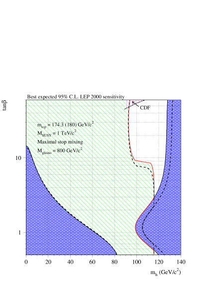
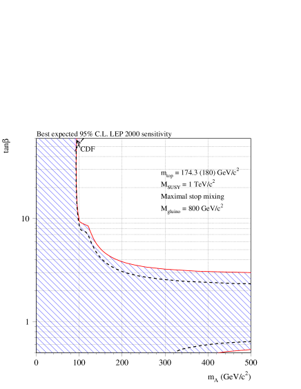
From fig. 11 and , it follows that, independent of the value of , LEP2 will be sensitive to a light Higgs boson with a mass up to about 93 GeV pjanot , depending slightly on the final luminosity collected. For low values of , the coverage is better and the search will cover up to the theoretically largest allowed value of the lightest Higgs mass, which is obtained for large values of the CP-odd Higgs mass. In this decoupling limit, the lightest Higgs has SM-like properties. The maximal LEP2 reach for a light Higgs with SM-like couplings to the boson is the same as the SM one, namely up to a mass of about 112 GeV for a discovery.
The anticipated final LEP lower bounds on the SM-like Higgs mass significantly constrain the MSSM parameter space. In particular, it is possible to derive a lower bound on as a function of the stop masses and mixing angles. As an example, fig. 12 shows the bounds on that will be obtained in the case that no Higgs boson is found at LEP with a mass below 115 GeV in the channel. This figure illustrates that the lower bound on will range between about 2.3 and 5 depending on the value of the stop masses and mixing. It is interesting to note that even for very large values of the stop masses and mixing angles, the bound on resulting from the direct bound on the Higgs mass becomes stronger than the bound on that one can get by the requirement of perturbative consistency of the theory up to scales of order (associated with the infrared fixed point solution of the top Yukawa coupling) CCPW . The constraints on the MSSM parameters that will be available from Higgs searches after the final run of LEP2 will be useful for guiding supersymmetric and Higgs particle searches at the Tevatron and the LHC.

One of the goals of the Tevatron Higgs Working Group is to examine the potential for the upgraded Tevatron to extend the LEP2 MSSM Higgs search. We begin by examining the most promising channels for MSSM Higgs discovery at the upgraded Tevatron.
I.3.5 MSSM Higgs Boson Decay Modes
In the MSSM, we must consider the decay properties of three neutral Higgs bosons (, and ) and one charged Higgs pair (). In the region of parameter space where and the masses of supersymmetric particles are large, the decoupling limit applies, and we find that the properties of are indistinguishable from the Standard Model Higgs boson.202020If supersymmetric particles are light, then the decoupling limit does not strictly apply even in the limit of . In particular, the branching ratios are modified, if the decays of into supersymmetric particles are kinematically allowed. In addition, if light superpartners exist that can couple to photons and/or gluons, then the one-loop and decay rates would also deviate from the corresponding Standard Model Higgs decay rates due to the extra contribution of the light superpartners appearing in the loops. In this case, the discussion of Section I.A.2 applies, and the decay properties of are precisely those of the Standard Model Higgs boson. In this case, the heavier Higgs states, , and , are roughly mass degenerate and cannot be observed at the upgraded Tevatron.
For values of , all Higgs boson states lie below 200 GeV in mass, and could in principle be accessible at an upgraded Tevatron (given sufficient luminosity). In this parameter regime, there is a significant area of the parameter space in which none of the neutral Higgs boson decay properties approximates that of the Standard Model Higgs boson. For example, when is large, supersymmetry-breaking effects can significantly modify the and/or the decay rates with respect to those of the Standard Model Higgs boson. Additionally, the Higgs bosons can decay into new channels, either containing lighter Higgs bosons or supersymmetric particles. In the following, the decays of the neutral Higgs bosons , and (sometimes denoted collectively by ) and the decays of charged Higgs bosons are discussed with particular emphasis on differences from Standard Model expectations.
As discussed earlier (see fig. 11), if the Higgs boson has not yet been discovered by the time the upgraded Tevatron begins its run, then the anticipated LEP limits will rule out values of below about 2.5.212121LEP will not be able to rule out small values of in a narrow range of MSSM parameter space. However, theoretical arguments favor values of , so we do not consider further the possibility of . Thus, in the following discussion, two cases are considered to illustrate the difference between “low” and “high” : and 30.
a. Neutral Higgs Boson Decays
\\[0.2cm] In the MSSM, the decay modes , dominate the neutral Higgs decay modes for large , while for small they are important for neutral Higgs masses GeV as can be seen from fig. 13a–c. As in the Standard Model case, the QCD corrections hffsmqcd reduce the partial decay widths into quarks by about 50–75% as a result of the running quark masses, while they are moderate for decays into top quarks DSZ . The dominant Higgs propagator corrections of and can to a good approximation be absorbed into the effective mixing angle hffsusyprop . As explained above, as a consequence of this universal correction the coupling of to and can be strongly suppressed for small and large . For the decays into , the supersymmetric-QCD corrections hffsusy1l ; hffsusyqcd ; bfpt ; CMW1 ; eberl ; hffsusyprop ; loganetal can be very significant for large values of and . Their dominant effect manifests itself in the relation between and the Yukawa couplings [resulting in eqs. (37) and (38)]. The dominant electroweak corrections from higgsinos to enter in the same way. The remaining process-specific electroweak one-loop corrections are typically at the level of only a few percent hffsusy1l .


, \\[0.2cm] In the MSSM, the decays are suppressed by kinematics and by angle factors [eq. (I.3.1)]. Hence, these decays are less important than in the SM. Their branching ratios turn out to be sizeable only for small and moderate or in the decoupling regime, where the light scalar Higgs particle reaches the upper bound of its mass.
, \\[0.2cm] The gluonic (photonic) decays of the Higgs bosons reach branching ratios of () in the MSSM and are expected to be unimportant at the Tevatron. A light top squark can enhance the branching ratio when its coupling has the opposite sign to the top quark contribution, and it will reduce the branching ratio in this case.
In addition to the above decay modes, which also arise in the Standard Model, there exist new Higgs decay channels that involve scalars of the extended Higgs sector and supersymmetric final states. The unambiguous observation of these modes would clearly constitute direct evidence of new physics beyond the Standard Model.
; \\[0.2cm] The decay is kinematically possible only for small values of , which would seem to have been ruled out by the present LEP Higgs mass bounds. However, there may be small regions in the MSSM parameter space, in which this decay is still kinematically allowed, consistent with the LEP Higgs search. The one-loop radiatively corrected rate for has been computed in ref. htoaa .
For GeV, the decay modes , are significant in the MSSM only for a very small range of masses (as shown in fig. 13). However, the process is not kinematically possible given the present LEP bounds on . The present LEP limits on and also suggest that is ruled out, although there may be small regions of the MSSM parameter space (as noted above) in which this latter decay mode is still allowed. For completeness, we note that for values of , the branching ratio of is dominant for a Higgs mass range of . The dominant radiative corrections to this decay arise from the corrections to the self-interaction in the MSSM and are large 7 .
, ; \\[0.2cm] The decay modes , and are important for small below the threshold. Below the corresponding thresholds, decays into off-shell Higgs and gauge bosons turn out to be important especially for small 13 . However, the MSSM parameter space where these effects are important for the Tevatron Higgs search are close to being ruled out by the anticipated LEP limits. In particular, present LEP limits already imply that the two-body decays , are kinematically forbidden. Similarly, the decay can be relevant at the Tevatron only for GeV and near its experimental lower limit.
supersymmetric particles \\[0.2cm] Higgs decays into charginos, neutralinos and third-generation squarks and sleptons can become important, once they are kinematically allowed 13a . For Higgs masses below 130 GeV, the range of supersymmetric parameter space in which supersymmetric decays are dominant is rather narrow (when the current bounds on supersymmetric particle masses is taken into account). One interesting possibility is a significant branching ratio of , which could arise for values of near its upper theoretical limit (assuming the decay is kinematically possible). Such an invisible decay mode would clearly complicate the Higgs search at the Tevatron. Note that if supersymmetric particles are directly produced and observed at the Tevatron, then new sources of Higgs boson production (either in association with a supersymmetric particle or in the decay chains of supersymmetric particle decays) may exist scottkon .
b. Charged Higgs Boson Decays
The anticipated constraints on the MSSM Higgs parameter space from LEP (see fig. 11) restrict the possible values of and . Using the tree-level relation of eq. (9), it follows that GeV.222222Using the radiatively-corrected expression for the charged Higgs mass does not significantly change this estimate. Moreover, if no Higgs signal is found at LEP, will be constrained to be larger than roughly 2.5. As will be seen in the next section, the prospects for detecting charged Higgs bosons at the upgraded Tevatron are poor unless they are light enough to appear among the decay products of the top quark. In this case, production followed by (or ) provides the most promising mechanism for discovering a charged Higgs boson at the Tevatron. These decays are kinematically allowed when , implying that GeV. Thus, there is a relevant range of MSSM parameter space ( GeV and ) in which the charged Higgs boson of the MSSM is accessible to the Tevatron Higgs search.
However, one can take a broader view. In non-supersymmetric two-Higgs doublet models, the phenomenology of the Higgs sector depends on the pattern of Higgs couplings to fermion-pairs. Type-II two-Higgs doublet models possess the same Higgs-fermion couplings as in the MSSM. Models with a different Higgs-fermion coupling pattern can also be constructed. In non-supersymmetric two-Higgs-doublet models, all the Higgs masses and the angles and are independent parameters. Thus, the restrictions on the Higgs parameters derived above in the case of the MSSM Higgs sector do not apply in the more general non-supersymmetric model. and it is quite simple to extend the charged Higgs phenomenology of the MSSM to the more general case. Additional complications arise only when the neutral Higgs bosons of the model affect the production and/or decay modes of the charged Higgs boson. Furthermore, using present experimental and theoretical knowledge, the indirect lower bound on the charged Higgs mass coming from measurement of the inclusive decay is about 165 GeV bsga in the non-supersymmetric Type-II two-Higgs-doublets model. In the MSSM, no such limit exists for , since supersymmetric particles can be exchanged in loops contributing to decay; these effects can approximately cancel out the corresponding charged-Higgs exchange contribution in some regions of MSSM parameter space.
\\[0.2cm] Because charged Higgs couplings are proportional to fermion masses [see eq. (I.3.1)], the decays to third generation quarks and leptons are dominant. In particular, for (so that the channel is closed), is favored if , while is favored only if is small. Indeed, if . The branching fractions of the two-body decay modes of the charged Higgs boson are shown in fig. 13d as a function of , and also in fig. 14 as a function of for several values of . These results apply generally to Type-II two-Higgs doublet models. For — GeV, the decay is the dominant decay mode.
The results of fig. 13d and fig. 14 include QCD quantum effects in all decays when relevant, besides in the three body decay mode . The QCD radiative corrections have been computed in ref. chhiggsdecay . Their effect on the charged Higgs branching ratios may be significant only in the region of where the and decay modes are competitive or for sufficiently large values of for the decay mode . In principle, depending on the supersymmetric parameter space, virtual supersymmetric (SUSY) particle exchange can also influence the branching ratios. The computation of radiative SUSY-QCD and SUSY-electroweak loop effects to the width of can be found in refs. chhiggstotop and chhiggstotop2 . In particular, the latter includes the resummation of the large QCD quantum effects and the dominant contributions for SUSY quantum effects, which are those associated to the redefinition of the Yukawa couplings due to bottom mass corrections (as discussed in section I.B.3).
\\[0.2cm] The decay (where is an off-shell -quark) can become competitive (and even dominant) with respect to the two body fermion decays. Only the tree-level prediction has been displayed in fig. 14. QCD radiative corrections have been computed in ref. chhiggsdecay3 . It is found that the pure QCD corrections raise the decay width of by about , and the SUSY-QCD corrections (due to gluino and third generation squark exchanges) can be comparable or even larger than the pure QCD corrections in some regions of the MSSM parameter space.
\\[0.2cm] The decay is kinematically allowed only for charged Higgs bosons that are heavier than the top quark. Hence, this mode is not relevant for the mass region which is most likely to be accessible at the Tevatron. The related decays , , where the is off-shell, can be sizeable for small and bordjo . However, as discussed above, this region of the MSSM parameter space is expected to be ruled out by the end of the LEP run. In more general non-supersymmetric two Higgs doublet models, these modes could be present, although their predicted rates are more model dependent (depending on unconstrained parameters from the neutral Higgs sector).

supersymmetric particles \\[0.2cm] Charged Higgs decay into charginos/neutralinos, and third generation squarks and sleptons can be important once they are kinematically allowed. However, for (most relevant for Tevatron phenomenology), the area of MSSM parameter space in which the two-body supersymmetric decay modes are kinematically allowed is not large baeretal ; bordjo . Still, this scenario cannot be ruled out at present (the most likely supersymmetric decay mode is ).
I.3.6 MSSM Higgs Boson Production at the Tevatron
a. Neutral Higgs Boson Production Processes
, [] \\[0.2cm] Over most of the MSSM Higgs parameter space, one of the two CP-even Higgs bosons has very suppressed couplings to , while the other one couples to with Standard Model strength. For the latter scalar state, the process [ or ] can be important. Note that the CP-even scalar has SM like-couplings to the vector bosons in two cases: (i) in the decoupling regime for the lightest Higgs boson, where and (ii) for large and low , where . In either case, the corresponding scalar has a mass less than about 130 GeV. This behavior is evident from the total cross-section curves shown in fig. 15a,b. These cross-sections include first-order QCD corrections; the corresponding factors are approximately 30% 23 . The SUSY-QCD corrections due to the exchange of virtual squarks and gluinos are not included; these are known to be small djospi .


[, , ] \\[0.2cm] The gluon fusion processes are mediated by heavy top and bottom quark triangle loops and the corresponding supersymmetric partners 29a ; spiramssm ; 21 . Gluon fusion is the dominant neutral Higgs production mechanism at the Tevatron, even for large , with cross-sections ranging from – pb (for GeV), as shown in fig. 15. However, as in the case of the Standard Model Higgs boson, the dominant final states are overwhelmed by the huge QCD background of production. Hence, it is not possible to detect at the Tevatron. Only the decay modes may be promising for large , especially if the Higgs bosons are produced in association with a jet.
As in the case of the , the two-loop QCD corrections are dominated by soft and collinear gluon radiation for small in the MSSM 29 . The factor remains nearly the same after including squark loops, since the dominant soft and collinear gluon effects are universal, thus suppressing the (s)quark mass dependence 21 .
[ or ; , ] \\[0.2cm] As noted previously, one typically finds that one of the two CP-even Higgs bosons has very suppressed couplings to , while the other one couples to with Standard Model strength. The process (CP-even Higgs production via vector boson fusion, or ) can be significant only for the SM-like scalar state. In either case the corresponding scalar has a mass less than about 130 GeV. In this mass range, observation of the Higgs boson via this channel at the Tevatron will be extremely difficult. The corresponding cross-sections are shown in fig. 15a,b. These cross-sections include first-order QCD corrections; the corresponding factors are small, enhancing the cross-section by roughly 10% 32 . The corresponding SUSY-QCD corrections are known to be small djospi , and are not included.
[, , ] \\[0.2cm] In the MSSM, Higgs boson radiation off bottom quarks becomes important for large with cross-sections of order 1 pb for and with masses of order 100 GeV and 0.1 pb for and with masses of order 200 GeV, see fig. 15. Thus, the theoretical predictions, including full NLO computations, are crucial to do realistic simulations of the MSSM Higgs signals in these channels.232323As mentioned in the corresponding discussion for , [see Section I.B.3], one also needs to evaluate and with suitable subtraction of the logarithms due to quasi-on-shell quark exchange (to avoid double counting) in order to obtain the total inclusive cross-section for production. For example, the enhancement can lead to copious -channel production of Higgs bosons via -quark fusion bhy . A complete calculation of this type, fully consistent up to does not yet exist in the literature. Moreover, as discussed in Section I.B.3, SUSY-QCD and SUSY-electroweak corrections to the coupling as those shown in eqs. (35), (37) and (38) play a very important role in enhancing or suppressing (depending on the exact supersymmetric spectrum) these production cross-sections at large CMW1 ; CMW2 ; bdhty .
Higgs Boson Pair Production \\[0.2cm] Light scalar Higgs pair production yields a cross-section at the Tevatron with fb 33 ; 34 . The cross-section for is of similar size in some regions of the MSSM parameter space [see fig. 16]. Since the process is sensitive to the trilinear coupling it is important for a partial reconstruction of the Higgs potential. One may hope that the dominant final states can be extracted from the QCD backgrounds due to the different event topologies. The two-loop QCD corrections have recently been calculated [for initial states in the limit of heavy top quarks, thus leading to a reliable result for small ]. They enhance the production cross-sections by about 70–90% and the Drell–Yan-like cross-section by about 30% 34 . SUSY-QCD corrections, considered in ref. djospi , are small and not included here.

b. Charged Higgs Boson Production Processes
\\[0.2cm] If , then the charged Higgs boson can be produced in the decay of the top quark via (and ) Roy1 ; Roy2 ; TDECAY ; bordjo . The decay mode can be competitive with the dominant Standard Model decay mode, , depending on the value of . Here, the case of a general Type-II two-Higgs doublet model [based on the Higgs-fermion couplings of eq. (I.3.1)] is considered. Since the Higgs sector of the MSSM is a Type-II two-Higgs-doublet model, the following considerations also apply to the MSSM under the assumption that there are no open charged Higgs decay channels into supersymmetric final states, i.e. . Fig. 17 shows the branching fraction as a function of for various choices of . Note that is significant for very small or very large values of , while it is suppressed for intermediate values of .


The results of fig. 17(a) incorporate one-loop QCD corrections (first computed in ref. toptochhiggsdecay ) and are thus applicable to the general Type-II two-Higgs doublet model. The QCD corrections to the branching ratio are sizeable for values of . In the MSSM, one-loop virtual supersymmetric particle exchange can also significantly influence the top quark branching ratios, depending on the choice of supersymmetric parameters. As an example, in fig. 17(b), the effects of one-loop MSSM radiative corrections is exhibited by the dashed lines for the case of GeV and the following supersymmetric parameters: TeV and GeV. The upper [lower] dashed curve corresponds to a negative [positive] value of and positive [negative] values of and . A full one-loop calculation of in the MSSM including all sources of large Yukawa couplings was presented in Ref susytoptochhiggsdecay . As explained in section I.B.3, the dominant SUSY-QCD corrections (due to gluino exchange) and SUSY-electroweak corrections are those associated with the redefinition of the Yukawa couplings due to -quark mass renormalization effects. A treatment including resummation of the leading QCD quantum effects and the dominant contributions from loop effects arising from supersymmetric particle exchange can be found in ref. chhiggstotop2 .
The total cross-section for charged Higgs production in the mass region under consideration is then given by:
| (42) |
With pb at TeV ttbarxsec , roughly 1400 events per detector will be produced in Run 2 of the Tevatron. Folding in the top quark branching ratio given in fig. 17, it is a simple matter to compute the inclusive charged Higgs cross-section for . For larger values of , the top quark that produces the charged Higgs boson must be off-shell, and one must compute the full processes and . This computation will be described in the next section. Note that if one evaluates in the region of , one obtains the single charged Higgs inclusive cross-section, (which is plotted in fig. 18242424In this computation, the renormalization and factorization scales have been chosen to be .), rather than full charged Higgs inclusive cross-section of eq. (42).252525The latter is not quite a factor of two larger than the former since can contain a charged Higgs boson; one must subtract off to avoid double-counting. As expected, in the region of , the single inclusive charged Higgs cross-section is completely dominated by on-shell production followed by the decay of one of the top quarks into a charged Higgs boson.

; , \\[0.2cm] If , then charged Higgs boson production occurs mainly through radiation off a third generation quark. Single charged Higgs associated production proceeds via the partonic processes (and the charge conjugate final state). As in the case of production, large logarithms arise for due to quasi-on-shell -channel quark exchanges, which can be resummed by absorbing them into the -quark parton densities. Thus, the proper procedure for computing the charged Higgs production cross-section is to add the cross-sections for and and subtract out the large logarithms accordingly from the calculation of the process soper ; OT . This procedure avoids double-counting of the large logarithms at , and correctly resums the leading logs to all orders. In particular, the contribution to the total cross-section coming from the kinematical region of the gluon-initiated process in which one of the two gluons splits into a pair of -quarks (one of which is collinear with the initial proton or antiproton), is incorporated into the -quark parton density. A cruder calculation would omit the contribution of the process and simply include the results of the unsubtracted process. The latter procedure would miss the resummed leading logs that are incorporated into the -quark density. However, the numerical difference between the two procedures is significant only for .
The single inclusive charged Higgs cross-section at the Tevatron is shown in fig. 18(a) as a function of the charged Higgs mass, for . These results are based on the calculations of refs. chhiggstotop and francesca and include the contributions of the process and suitably subtracted process as described above. Fig. 18(b) depicts the single inclusive charged Higgs cross-section as a function of , for and GeV. In the computations that produced these two figures, the solid lines correspond to the prediction of a general two-Higgs doublet model (without supersymmetry). Only tree-level diagrams are evaluated, with the Higgs–fermion Yukawa coupling determined by a -quark mass which is varied in the interval 2.5 GeV GeV (corresponding to the shaded band). The renormalization and factorization scales were fixed at the threshold value . The variation of these scales would change the values of the cross-section presented here. For example, a variation in the interval between and , can produce deviations up to with respect to the values shown in the figures. In low-energy supersymmetric models, the effects of the leading SUSY-electroweak corrections can significantly modify the tree-level vertex depending on the values of the MSSM parameters. This is illustrated by the dashed lines in fig. 18 which are displaced from the corresponding solid lines due to the virtual supersymmetric effects.262626The leading MSSM effects shown in fig. 18 have been implemented only in the computation of the process, , . The effects displayed correspond to the following supersymmetric parameters: GeV, GeV, GeV, GeV, and GeV. The upper [lower] dashed curve corresponds to a positive [negative] value of .
, \\[0.2cm] Pair production of charged Higgs bosons occurs via Drell-Yan annihilation. The dominant contribution, which arises from the annihilation of and quarks into a virtual photon or , is independent of . Some dependence enters through annihilation via -channel top-quark exchange, although this effect is more than one order of magnitude suppressed relative to the dominant contribution. The tree-level result for for TeV, taken from ref. kniehl1 , is shown in fig. 19. These results are obtained with the Higgs–fermion Yukawa coupling based on a fixed -quark pole mass of GeV. Note that the inclusive cross-section lies below the cross-section for single charged Higgs associated production (see fig. 18) over the entire Higgs mass range shown.
, \\[0.2cm] Associated production of a charged Higgs boson and a can occur via annihilation and -fusion kniehl2 . The contribution of annihilation to (both charge state pairs are included) is shown as function of the charged Higgs mass for and 30 in fig. 19. The annihilation always dominates over -fusion except in the parameter regime where is close to one and the charged Higgs mass is greater than about 200 GeV. The fusion contribution is greatly suppressed if , independent of the value of the charged Higgs mass.
Given the small number of events predicted (before cuts, efficiencies and backgrounds are taken into account), it seems unlikely that this process would provide a charged Higgs discovery signature at the Tevatron.

I.4 New Higgs Physics Beyond the Standard Model/MSSM
In the previous section, the particular case of the Minimal Supersymmetric Standard Model was discussed in great detail. A more agnostic approach to the study of physics beyond the Standard Model is to construct an effective Lagrangian. The effective Lagrangian is a model–independent approach that describes the effects of new physics associated with an energy scale which lies beyond the scale where experiments are performed. The effective Lagrangian can be constructed out of higher dimensional (hence non–renormalizable) operators and depends only on the particle content of the low energy theory. The discussion of this section is limited to the case of having a light Higgs boson contained in these operators. Hence, a linearly realized linear ; hisz invariant effective Lagrangian is assumed to describe the bosonic sector of the SM, keeping the fermionic sector unchanged.
There are eleven dimension–6 operators involving the gauge bosons and the Higgs scalar field which respect local , and symmetries linear . Six of these operators either affect only the Higgs self–interactions or contribute to the gauge boson two–point functions at tree level and are severely constrained from low energy physics below the present sensitivity of high energy experiments hisz . From the remaining five “blind” operators, four affect the Higgs couplings and can be written as linear ; hisz ,
| (43) |
where is the Higgs field doublet, , and with and being the field strength tensors of the and gauge fields respectively. Anomalous , , and couplings are generated by Eq. (43), which modify the Higgs boson production and decay hagiwara2 . In the unitary gauge they are given by
where . The effective couplings , , and and are related to the coefficients of the operators appearing in Eq. (43) and can be found elsewhere hagiwara2 . Of special interest is the Higgs couplings to two photons, which is given by
| (44) |
Eq. (43) also generates new contributions to the triple gauge boson vertex linear ; hisz . The operators proportional to give rise to both anomalous Higgs–gauge boson couplings and to new triple and quartic gauge boson self–couplings. On the other hand, the operators proportional to and only affect couplings and cannot be constrained by the study of anomalous trilinear gauge boson couplings.
A summary of the present bounds on the couplings introduced in eqs. (43)–(I.4) from searches at the Tevatron and LEP, and an analysis of the possible bounds attainable at the upgraded Tevatron will be discussed in Section III.C.
New physics can also modify the couplings of Higgs bosons to fermions. For example, in the topcolor model chill the coupling of a composite charged Higgs boson to charm and bottom quarks can be so large that the signal of the charged Higgs boson via the -channel process is spectacular bhy . A similar conclusion applies to the generic type-III two-Higgs-doublet model, in which both Higgs doublets couple to up-type and down-type fermions.272727Constraints on Type-III two-Higgs doublet models have been recently addressed in ref. typethree .
One can develop a more model independent approach for the effects of new physics on fermion–Higgs boson couplings by following the chiral Lagrangian methods as in the case of the vector boson–Higgs boson couplings discussed above. Such a generic analysis has yet to be applied to the Tevatron search for Higgs bosons.
II Experimental Studies
II.1 The Tevatron in Run 2
In the next run of the Tevatron collider, with the new Main Injector and Antiproton Recycler, the machine will deliver more than an order of magnitude more instantaneous luminosity, and ultimately more than two orders of magnitude integrated luminosity to the CDF and DØ experiments. This prospect greatly enhances the discovery potential for new particles, since more integrated luminosity translates into more sensitivity at higher masses. As will be seen below, this is particularly important for the search for the Higgs boson, since the discovery reach is limited by statistics.
In Run 1 the Tevatron operated with six proton and six antiproton bunches, colliding every 3.5 sec. Instantaneous luminosities at the beginning of each store typically reached 1.61031/cm2/sec, or about 2 pb-1 per week integrated luminosity delivered to the experiments. The main limitations were in the proton and antiproton beam currents, and the antiproton stacking rate.
In Run 2 the new Main Injector will provide emittance much better matched with that of the Tevatron, greatly improving the antiproton transfer efficiency to the Tevatron, and also will give a threefold increase in the antiproton production rate. At the end of each Tevatron store, beams will be decelerated and the antiprotons extracted into the new Antiproton Recycler, and re-used in the subsequent store. This will effectively double the antiproton stacking rate.
In addition the Tevatron will switch to 36-bunch operations, which will greatly alleviate the problem of multiple interactions, keeping it at roughly the same level as in Run 1. The machine energy will increase from 1.8 TeV to 2.0 TeV in the center of mass; this typically increases physics cross sections by about 30-40%.
The initial goal of Run 2 (called Run 2a) is to deliver 2 fb-1 by then end of 2002, with instantaneous luminosities of up to 21032/cm2/sec. With 3636 bunches the crossing time will be 396 nsec; however both CDF and DØ have reconfigured their front-end electronics to accommodate 132-nsec crossing times, since with subsequent improvements the Tevatron will operate with more bunches, with this collision crossing time.
Further improvements to the luminosity will require successful research and development in the areas of improved antiproton availability and controlling the effect of the beam-beam interaction. If these lead to luminosities in the range of 51032/cm2/sec, then in Run 2b the Tevatron could deliver 15 fb-1 by then end of 2007 holmes .
This report presents results of feasibility studies for Higgs searches at the Tevatron during the upcoming data taking. During Run 1, initial Higgs searches were made by both CDF juano ; cdfrun1higgs and DØhobbsfit . Figure 20 shows the Run 1 Standard Model Higgs cross section limits from CDF in each final state studied and also the limit obtained by combining all channels. In addition to the Run 1 experimental results, initial Run 2 feasibility studies were performed in refs. tev2k ; snowmass96 ; tev33 . These studies considered production of the Standard Model Higgs boson with GeV, and concluded that was needed to discover a 120 GeV Higgs boson at the level. The present study improves upon the existing work in a number of significant ways. In this report, a improved background analysis and a more realistic detector simulation has been employed. In addition, results from all the leading channels were combined, and new channels relevant for the search for Higgs bosons of higher mass were examined. We first discuss in detail the simulation and analysis methods used in this report. We then focus on the search for the Standard Model Higgs boson in a variety of channels. Finally, we consider new search techniques relevant for Higgs bosons that arise in theories beyond the Standard Model.
II.2 Simulation and Analysis Methods
The goal of the Higgs Group experimental studies is to estimate the discovery reach for the Standard Model and MSSM Higgs bosons in Run 2 and beyond at the Tevatron. This is ultimately expressed in terms of the integrated luminosity required to either exclude the Higgs with 95% confidence if it does not exist, or discover it with some statistical significance, or for example, if it does exist at some mass.
Both CDF and DØ will be significantly upgraded in Run 2, and among the most significant enhancements relevant for the Higgs search are
-
•
three-dimensional charged particle tracking in both experiments,
-
•
precise silicon vertex detectors for heavy quark tagging,
-
•
charged track triggering using the silicon detectors,
-
•
efficient electron and muon identification over the central and forward regions, and
-
•
good jet energy resolution with multiple detector elements.
Estimating the integrated luminosity thresholds requires knowledge of the signal production cross section and acceptance, identification efficiencies, and backgrounds. At the time of the Workshop, neither CDF nor DØ has had full simulation programs of the detector available. The Workshop participants agreed to estimate the Higgs reach based on an average of the expected CDF and DØ detector performance, as represented in a simple simulation, called SHW, described below.
Also, neither the final -tagging efficiency nor the mass resolution for Run 2 is known, and part of the motivation for the Workshop was to determine the potential gain from future work on these very important factors in the Higgs reach. Studies of the tagging efficiency and mass resolution are presented below, and serve as the basis for the assumptions made in the individual signal channel studies and in the SHW simulation program.
We emphasize, however, that obtaining optimal -tagging efficiency, Higgs mass resolution, and experimental backgrounds will ultimately rely, in each experiment, upon detailed studies of the data to be collected in Run 2. Our aim is to show how the final results depend on these crucial factors, with reasonably optimistic projections for what we might ultimately attain with a great deal of hard work in the coming years.
II.2.1 SHW Simulation
John Conway, Ray Culbertson, Regina Demina, Ben Kilminster, Mark Kruse, Cal Loomis, Konstantin Matchev, Maria Roco \\
The SHW simulation provides a simple simulation of the “average” detector response of the upgraded CDF and DØ detectors. The program provides an interface to the ISAJET ISAJET and PYTHIA PYTHIA Monte Carlo programs, and stores events (internally and externally) using the STDHEP package. SHW thus provides a simple interface to these Monte Carlo programs, allowing people to perform event generation, simple detector simulation, and event analysis in the same program.
A parameterized simulation such as this, by its nature, will not fully simulate all the effects of the real detectors. But this program provides a reasonably close approximation for signal and background acceptance studies, and allows the most promising channels and analyses to be compared. Where possible, the results presented in subsequent sections are compared with actual data and extrapolations of the full Run 1 detector simulation. The good agreement found in these comparisons gives confidence that the SHW simulation is accurate enough for the studies in this Workshop, considering the uncertainties in detector performance and reconstruction techniques.
SHW begins by generating events (or reading events from a file), and then determining what charged tracks and calorimeter energy deposits the detector would record. From that information the program then makes lists of trigger and reconstructed “objects” including high-ET photons, electrons, muons, hadronically decaying taus, jets (including - and -jet tagging), and heavy stable charged particles. The user of the program can put her/his event analysis code in a routine called from within this framework.
The simulation implemented in SHW operates by taking the list of generated final state particles, and for each one simulating the response of the detector in terms of charged particle tracking and calorimeter energy deposits. This information, in turn, is used to perform particle identification much as in the actual experimental data analyses.
Tracking \\
A final state charged particle will leave a track which can be reconstructed with high efficiency if it traverses the central region of the detector. The SHW package does not simulate magnetic deflection, which is very small for high- tracks (such as energetic leptons) and does not contribute significantly to the uncertainty in the reconstruction of jet energies. Any final state charged particle with and MeV/ is assumed to have a 97% probability of producing a track, which is recorded in the track list. Track momentum resolution is simulated by including Gaussian smearing in sagitta simulated as if the track were in a 1.4 Tesla magnetic field. The gaussian width comes from assuming a 1-meter tracker with a resolution of 0.08%/GeV at high .
Calorimetry \\
The calorimeter represented by SHW is segmented in a number of cells in eta and phi, controlled by parameters in the include file. Both the size of the cells and the range of coverage in pseudorapidity are set by these parameters. The default was 28 cells in azimuth, and 80 cells in the pseudorapidity range , reflecting an “average” of the CDF and DØ calorimeter segmentations.
Each calorimeter tower has an electromagnetic section and a hadronic section, in which some fraction of a particle’s energy is deposited. The response of the calorimeter in the Run 1 simulation programs provides the basis for determining how much energy each particle deposits in a calorimeter tower. For example, using a Monte Carlo simulation of single pions, it is determined that on average 25% of the energy is deposited (about half of the time; the rest of the time no energy is deposited) in the electromagnetic section, and the rest in the hadronic section. The single pion simulation shows also that in about 5% of cases the particle passes through the non-instrumented region between calorimeter cells (“cracks“).
The energy resolution of the electromagnetic calorimeter is assumed to be 20%/, with in GeV, for photons and electrons, and 80%/ for hadrons. Muons deposit minimum-ionizing energy of 0.5 GeV in the electromagnetic calorimeter, and 2.5 GeV in the hadronic calorimeter. The program assumes that a given particle deposits all its energy in a single cell.
Figure 21 shows the electromagnetic and hadronic calorimeter response as a function of incident particle energy for a CDF Monte Carlo simulation of single electrons, muons, and pions. These distributions motivate the choice of parameters in the SHW calorimeter simulation.


Once calorimeter tower energies are determined, the program performs a simple clustering algorithm, assigning towers with energy deposits to one of a list of calorimeter clusters formed from scanning the calorimeter tower energy array iteratively for the tower with maximum , and adding to the cluster thus formed any tower with energy above threshold and within =0.4, where .
The program also calculates the total missing from the individual calorimeter towers, performing a vector sum of the individual tower energies in the transverse plane.
Trigger \\
The CDF and DØ triggers rely on using fast information from the tracking and calorimeter to signal the presence of photons, leptons, jets, missing , etc. The SHW simulation uses the list of charged tracks and calorimeter tower energy deposits to arrive at a list of trigger “objects” including electromagnetic deposits, jets, missing ET, etc. These can be required in combination to simulate the actual online triggers foreseen in Run 2.
Physics objects \\
Typical analyses at hadron colliders begin by identifying photons, electrons, muons, hadronic taus, jets, and so forth and then demanding the presence of certain combinations of these objects depending on the final state to be selected. The SHW package performs this by making identification requirements on the calorimeter clusters, tracks, and raw calorimeter tower energies.
The simulation identifies photons and electrons by finding calorimeter towers with GeV in the range , having a ratio of hadronic to electromagnetic energy less than 0.125. The transverse energy in a cone of 0.4 around this tower must be less than 10% of that in the central tower. In the case of photons, there must be no track within , or one track if it has GeV/. For electrons, there must be a track within , and the highest such track must have . To simulate gaps between calorimeter cells, electrons and photons are dropped if they are near the calorimeter cell boundaries in .
Muons are identified by finding tracks coming from generated muons, and applying efficiency factors for fiducial coverage and typical reconstruction efficiency. The overall efficiency for muons is roughly 85%. No fake muons are generated from random tracks.
Hadronically decaying taus are identified by seeking calorimeter deposits in the region associated with one or three charged tracks within 10∘ of the calorimeter cluster centroid. Hadronic jets are rejected by demanding no other tracks in an annular region between 10∘ and 30∘ centered on the calorimeter cluster centroid. There must be at least one track with GeV/. Electrons are rejected by demanding that . The efficiency for hadronically decaying taus varies with the event jet environment from about 40% to 60%.
Jet clusters are formed from the list calorimeter tower energies. The algorithm seeks the maximum- tower not assigned to a cluster, then adds to the new cluster any adjacent towers within a specified cone in (default 0.4) around the seed tower. Jets can be tagged as - or -jets by first determining the true jet type by comparing the reconstructed jet with generated quark and gluon directions and energies.
There are two default algorithms available for heavy quark tagging, based on the CDF jet probability algorithm, and an algorithm which counts high-impact-parameter tracks in jets. The efficiencies for these algorithms are parametrized as a function of jet . Figure 22 shows the tagging rates per taggable jet for these parametrizations, for jets within the fiducial region.
Note, however, that some of the analyses presented in the following sections make use of parametrizations of the -tagging efficiency which differ from the default parametrizations in SHW. In this scheme there are “tight” and “loose” tagging efficiencies, as depicted in Figure 23. This algorithm is based on projections from the CDF Run 1 tagging rates, incorporating the improved vertexing possible with the new silicon detectors, and using both the secondary vertex (SECVTX) algorithm and soft lepton (SLT) tagging.
 \\
\\
 \\
\\

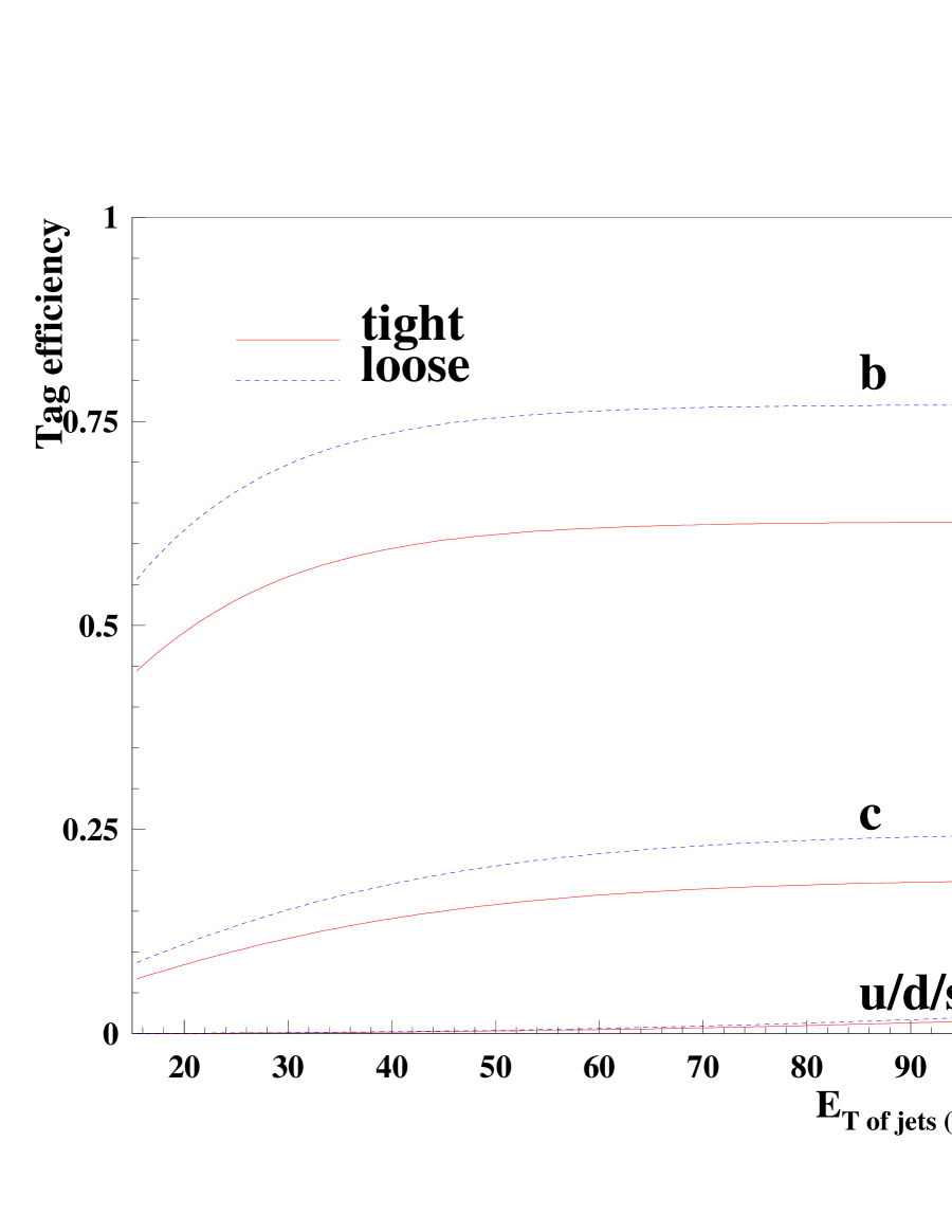
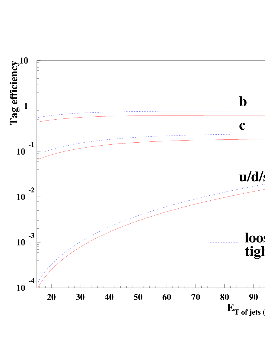
II.2.2 Study of Mass Resolution
T. Dorigo, S. Kuhlmann, R. Snihur, G. Watts, J. Womersley \\
For Higgs masses less than about 135 GeV the most promising channels in Run 2 at the Tevatron involve the decay of the Higgs to , such as the process . The signal is an excess of events having invariant mass peaked at the Higgs mass. Obtaining the best possible invariant mass resolution is therefore crucial in establishing a signal.
This section presents the results of two studies of the dijet mass resolution in the upgraded Run 2 detectors.
CDF Dijet Mass Resolution Studies \\
The decay of the Higgs boson dominates if . Our ability to extract this particle from the large QCD background in Run 2 (for instance in the final state, when associated production is sought) will therefore depend critically on the resolution we can attain on the Higgs boson mass, reconstructed from the measured -quark jet energies: both the possibility to see a bump in a dijet mass spectrum and the option to apply a mass window cut as a selection tool will strictly depend on the attainable mass resolution.
A study of jet–energy resolution in QCD dijet events with one electromagnetic jet was carried out by CDF. This study improved upon the calorimeter–only jet energy measurement typically used in Run 1 CDF (and DØ) analyses by including information from charged–particle momenta measurements and shower maximum detectors. Figure 24 shows the jet energy resolution for both the calorimeter–only jet energy algorithm and the improved algorithm. This shows roughly a 30% improvement in energy resolution.
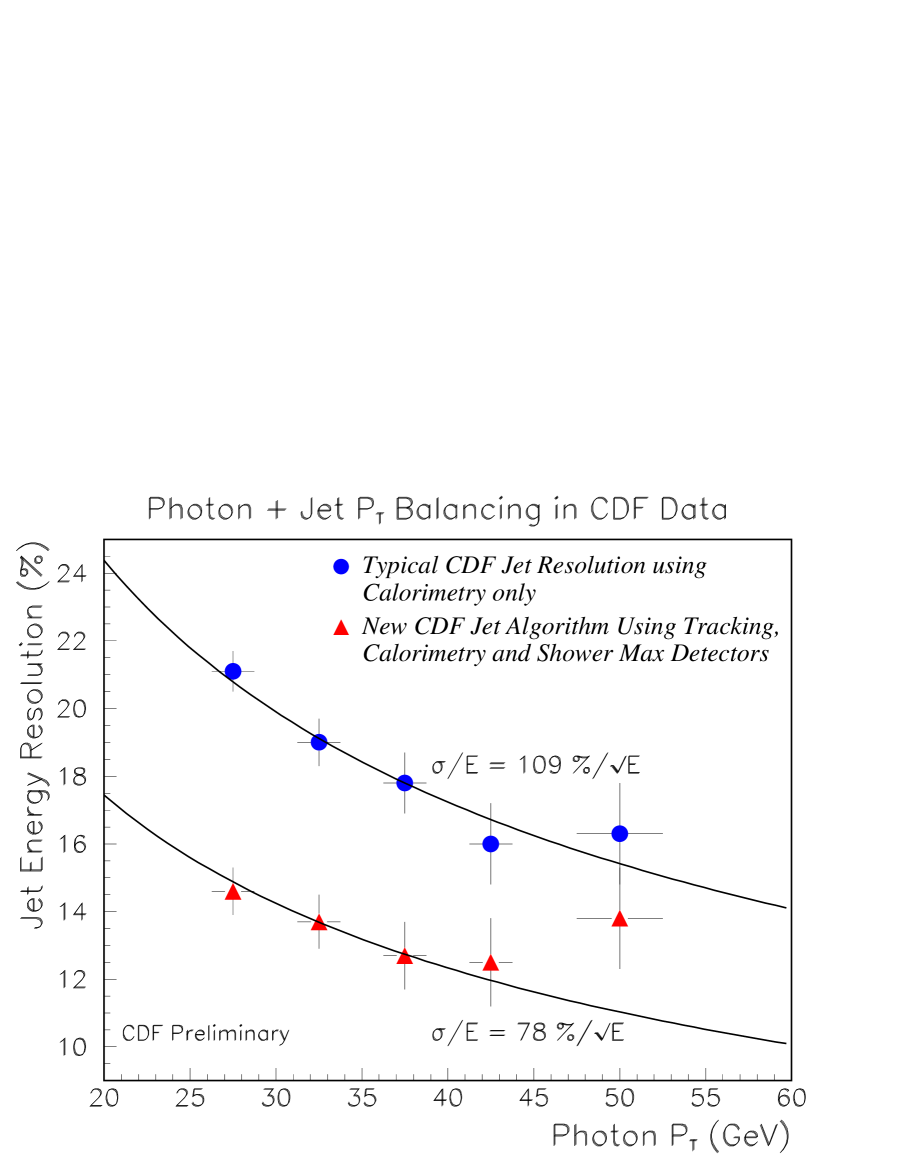
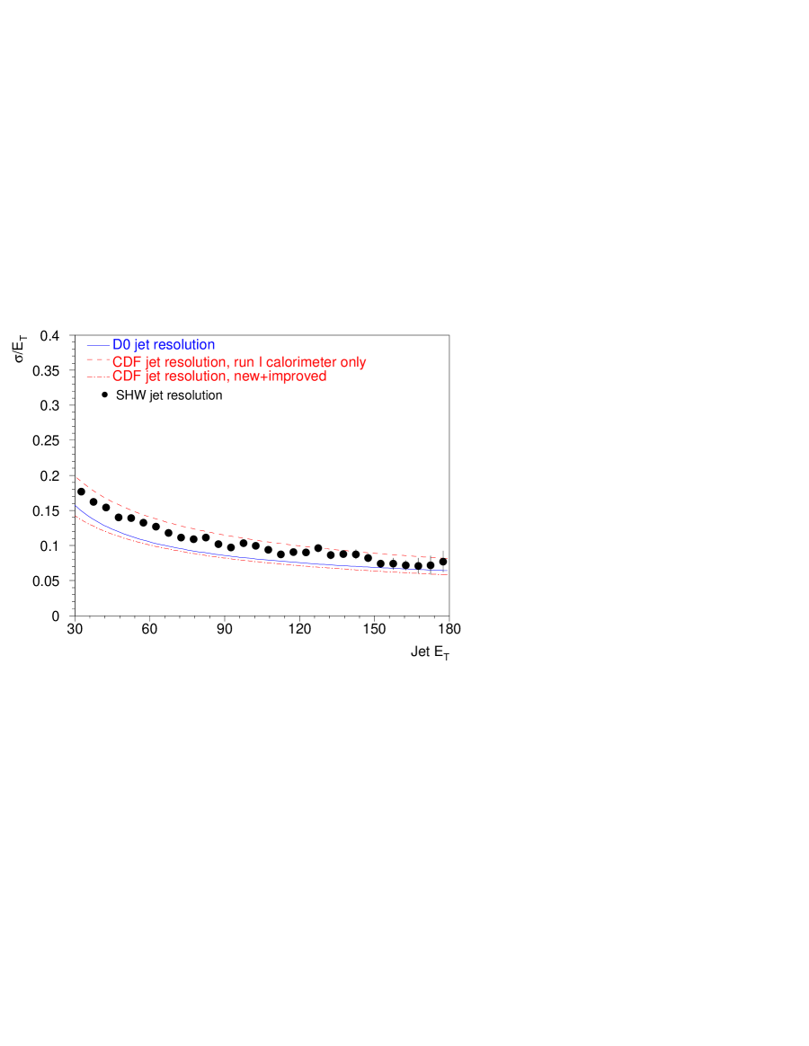
A study of the dijet mass resolution in events was performed by CDF in the context of a search for that process in events collected by an inclusive muon trigger. Two million decays were generated with the PYTHIA 5.7 Monte Carlo, and filtered as the data.
After the application of the standard CDF jet correction routine, many observable quantities were studied as a function of the difference between measured jet momenta and originating parton momenta, in the hope of using the measured values of these observables to help reducing the energy mismeasurement. The quantities that were found most useful for this purpose were the following: the muon momentum, the missing transverse energy projection along each jet, and the jet charged fraction.
The muon momentum is needed in correcting the energy of jets originating from the semileptonic decays of -quarks, because the minimum ionizing muons do not contribute linearly to the energy measured in the calorimeter. The missing , projected along the direction of the jets in the transverse plane, provides useful information on the momentum taken away by the neutrino and on a possible fluctuation of the energy measurement. The charged fraction of the jets (defined as the ratio between the total momentum of reconstructed charged tracks inside the jet cone and the jet momentum measured in the calorimeter) also helps reduce the uncertainty in the energy measurement.
By properly accounting for the value of these observables, it was possible to reduce the relative width of the dijet mass distribution, , by nearly (see Figure 25, left).
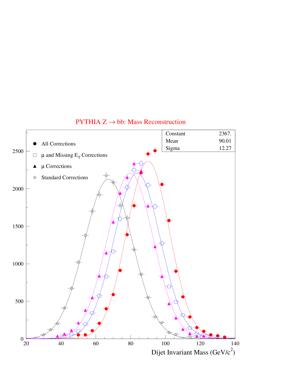
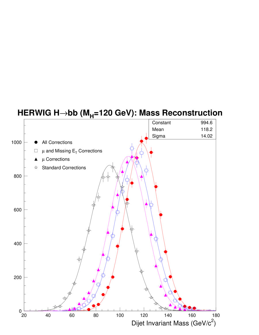
The validity of these corrections was tested with HERWIG herwig to check the effect of a different fragmentation model, and no differences were found. The corrections were also checked on a simulated sample of decays, with , and were found to be equally useful for a different resonance mass (Figure 25, right).
Finally, it was possible to show that a real sample of decays extracted from Run 1 data behaved as expected from the simulation: the reconstructed excess of events over background predictions indeed showed an average value and width in agreement with Monte Carlo predictions both before and after the application of the jet corrections (Figure 26).
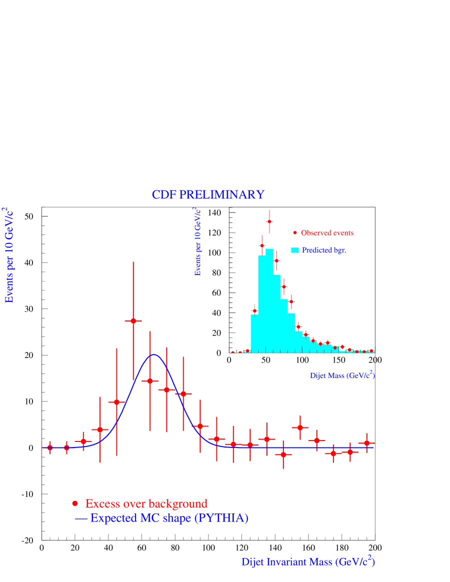
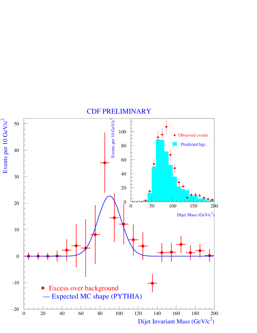
The corrections described above were specifically intended for a pair of back-to-back -quarks, when one of the two decays to a muon. Their success in improving the significance of the signal, however, demonstrates the usefulness of the chosen approach, and spurs new studies aimed at different final state topologies for the search for new resonances.
DØ Dijet Mass Study \\
This study is based on events generated using PYTHIA with a Higgs mass of 90 GeV simulated in the DØ detector. The decay was forced to in order to give a relatively “clean” dijet Higgs signal in the calorimeter. Events were generated with both initial and final state radiation (ISR and FSR) as default, but we also generated samples with neither ISR nor FSR, with only ISR, and with only FSR, for comparison purposes. Events were then passed through the D0GEANT detector simulation which provides a full simulation of the calorimeter response and resolution. (This is the Run 1, fortran-based detector simulation). The digitized events were then passed through the Run 1 calorimeter reconstruction and jet finding packages.
In the analyses presented here, we required the following standard jet selection cuts:
The reconstructed mass distributions were characterized using a fit function formed of a gaussian convoluted with two exponentials hobbsfit . The fits typically yield a per degree of freedom between 1 and 2. The bin containing the peak and the bin separation corresponding to the FWHM were found by hand.
Two jet clustering algorithms were investigated. The first is the standard DØ cone algorithm, with a cone size of . The second is the algorithm, with parameter settings of 0.5 and 1.0 ( is a close approximation to the in the cone algorithm.) In the algorithm each hit calorimeter cell forms a vector. Vectors are combined with each other to build a jet by joining the two vectors with the smallest relative to form a new vector. Combination stops when all vectors are separated by ktalg .
Our attempt throughout this study is to demonstrate the factors governing mass resolution, rather than to present final results on the resolution that can be attained. Much work will have to be done in deriving energy scale corrections before final resolution numbers are finalized.
Parton, Particle and Calorimeter Level Resolutions \\
To demonstrate the effects of hadronization, radiation, and of the calorimeter energy measurement, we have applied the same algorithm at the parton, particle and calorimeter cell levels. We used the DØ Run 1 jet finder and excluded the muon and neutrino from the decay from the parton and particle level jets. Two values of the jet size parameter were used, 0.5 and 1.0. Figure 27 shows the mass resolution obtained at the parton level. Without any gluon radiation, the Higgs mass is reconstructed perfectly (left hand pane); gluon radiation degrades this somewhat, as shown in the right hand pane which has both initial state radiation (ISR) and final state radiation (FSR) included.
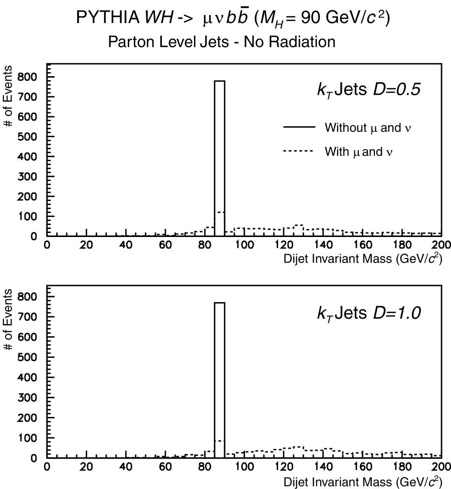
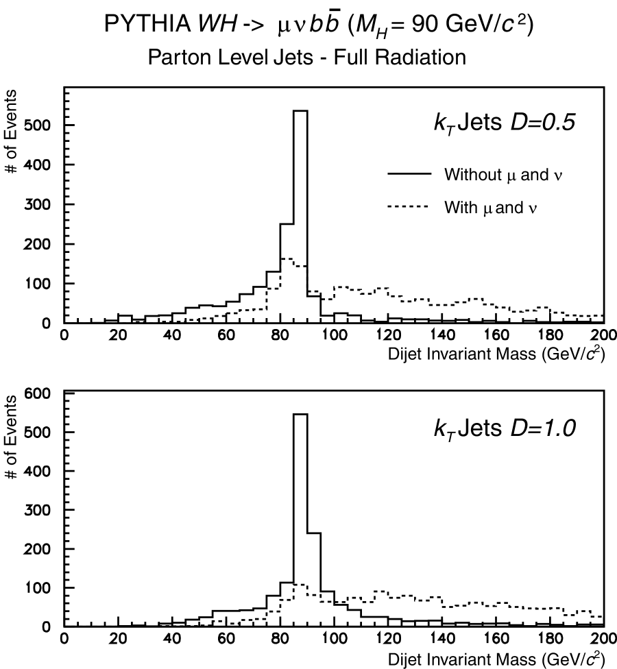
Hadronization introduces a low-side tail to the mass distributions, as may be seen in Figure 28; it is somewhat washed out when ISR and FSR are included. At this point the larger value starts to give a better resolution since it clusters more of the final state particles into the reconstructed jets.
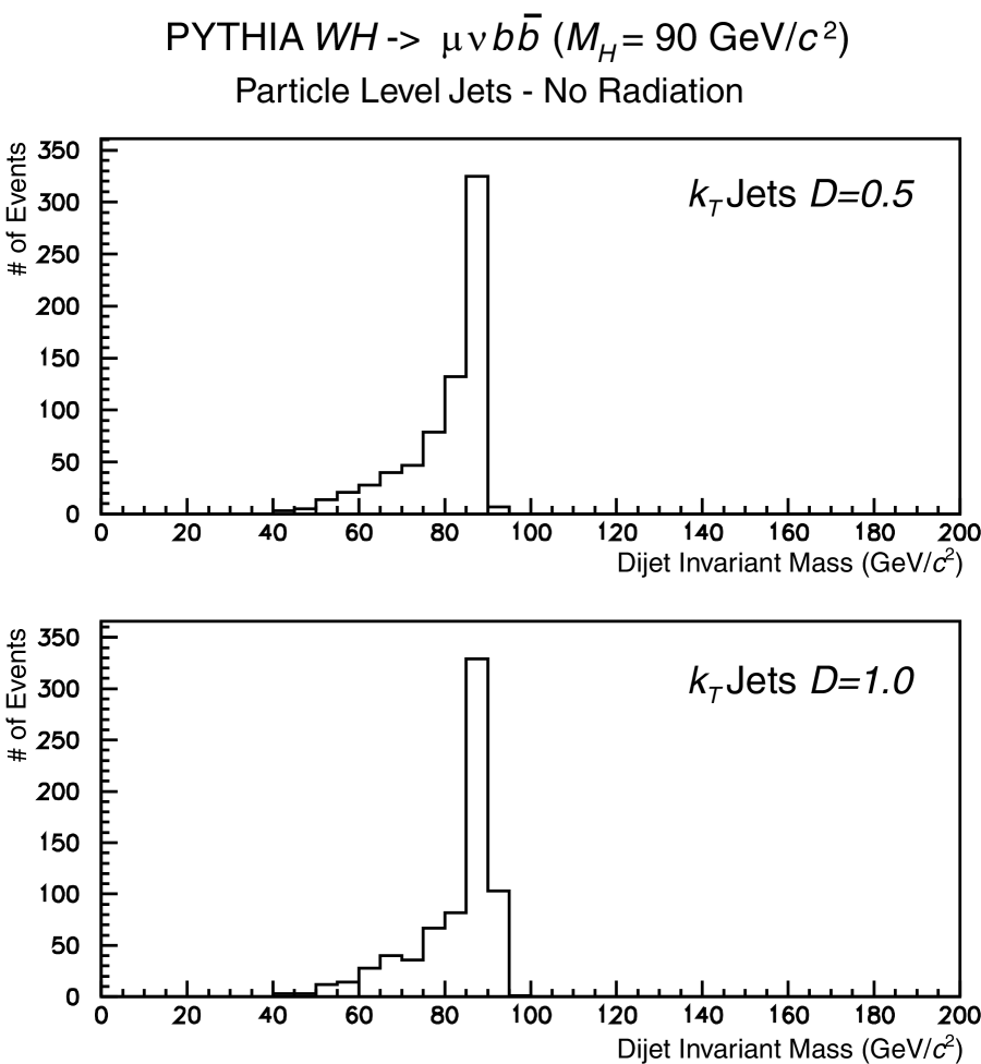
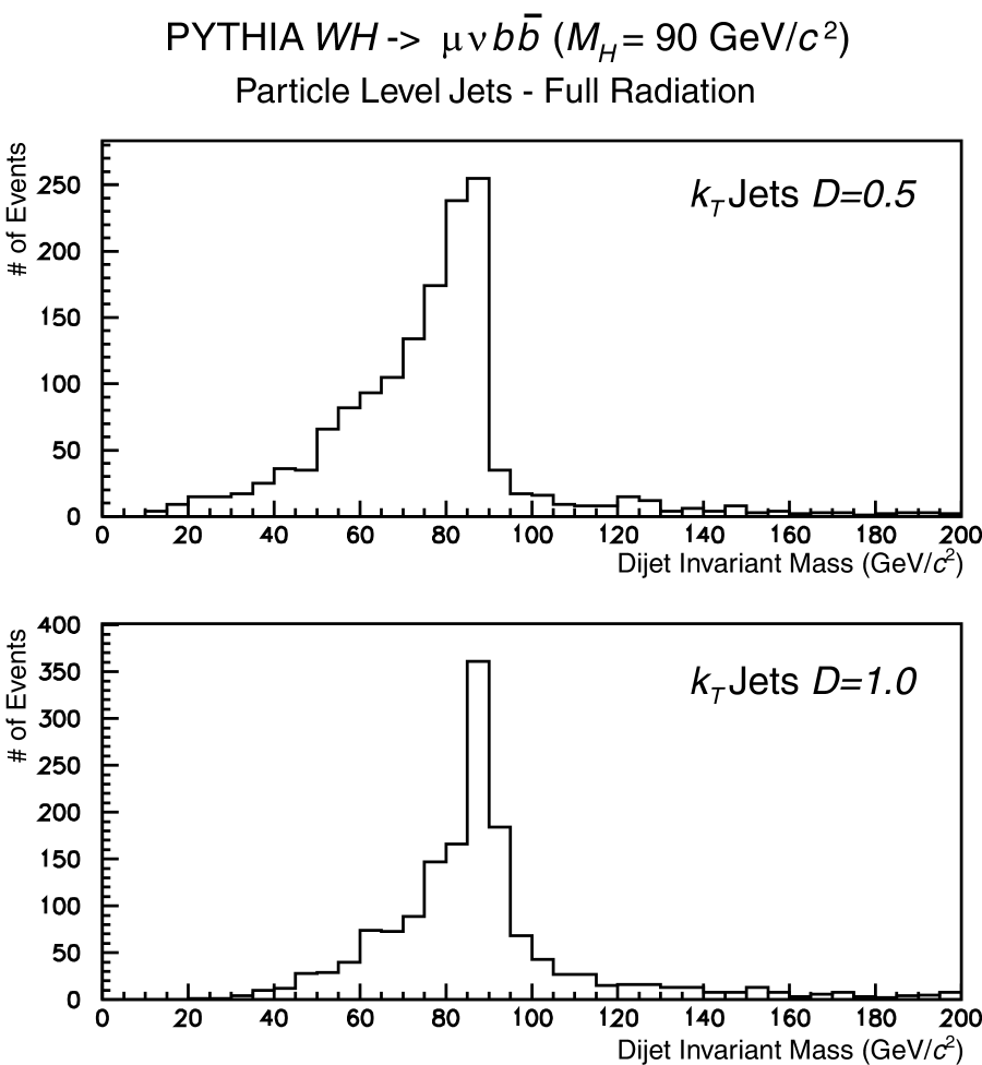
Finally at the calorimeter level we obtain the distributions in Figure 29 which correspond to what would be measured in the detector. We will now investigate the calorimeter level distributions in more detail.
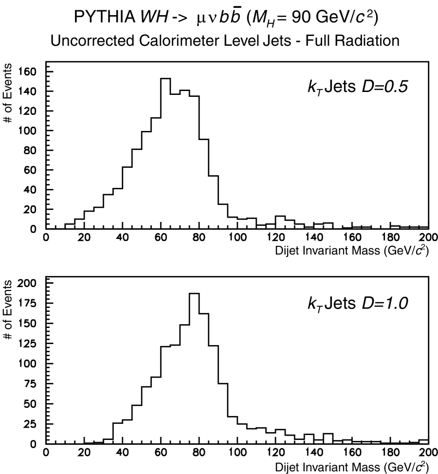
Dijet Mass Definition \\
We compared two different dijet mass estimators:
and
For the particular case of cone jets, and plotting the mass of the leading two jets in the event, the two quantities are shown in figure 30. They yield very similar fractional widths though they are not bin-by-bin identical. In most of what follows we shall use .

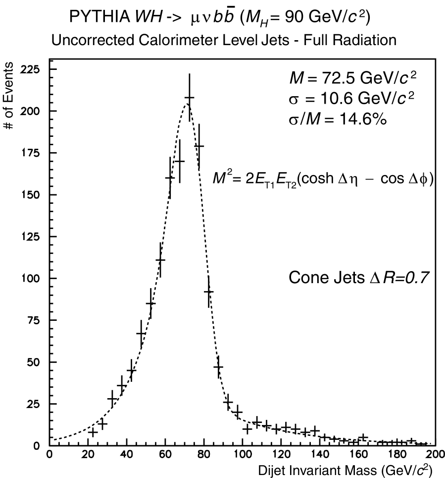
Energy Scale Corrections \\
We applied the DØ Run 1 jet energy scale corrections to the jets before forming the invariant mass. To our disappointment, the mass resolution was degraded about 10% by these “corrections”. This is perhaps not too surprising since the corrections were derived for jets at much higher and were also not optimized for -jets in any way. The DØ top mass analysis used a different set of jet corrections which would probably be more appropriate here, but these were not available in our analysis package. In what follows we shall use uncorrected jet energies.
Cone and Jets Compared \\
One of the hopes of using the algorithm was that the mass resolutions would be better. The algorithm should do a good job of recombining final state radiation with the parent parton jet because it recombines particles with a small invariant mass. The jet mass resolution shown in this paper is worse than the resolutions found by the cone jet algorithm except in the high luminosity case with . The mass resolutions from are larger than for the cone, as can be seen in Figure 31 for and 0.5. The larger value gives a better resolution and a peak mass closer to the true Higgs mass. A complete analysis of the jet mass resolution, including jet energy corrections, in progress at DØ.
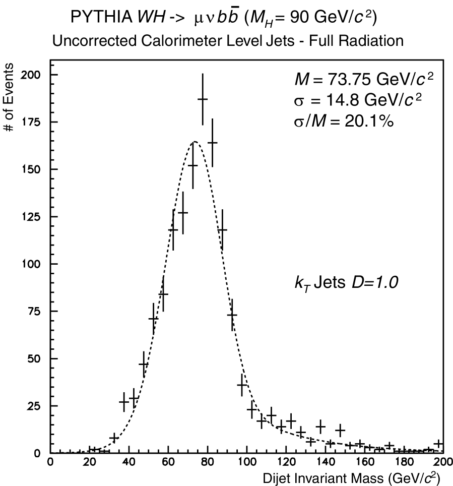
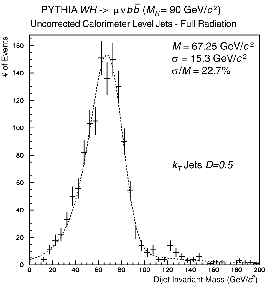
Initial and Final State Radiation \\
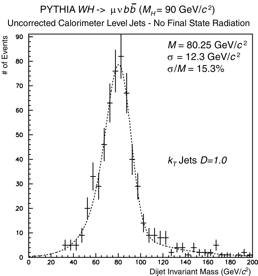
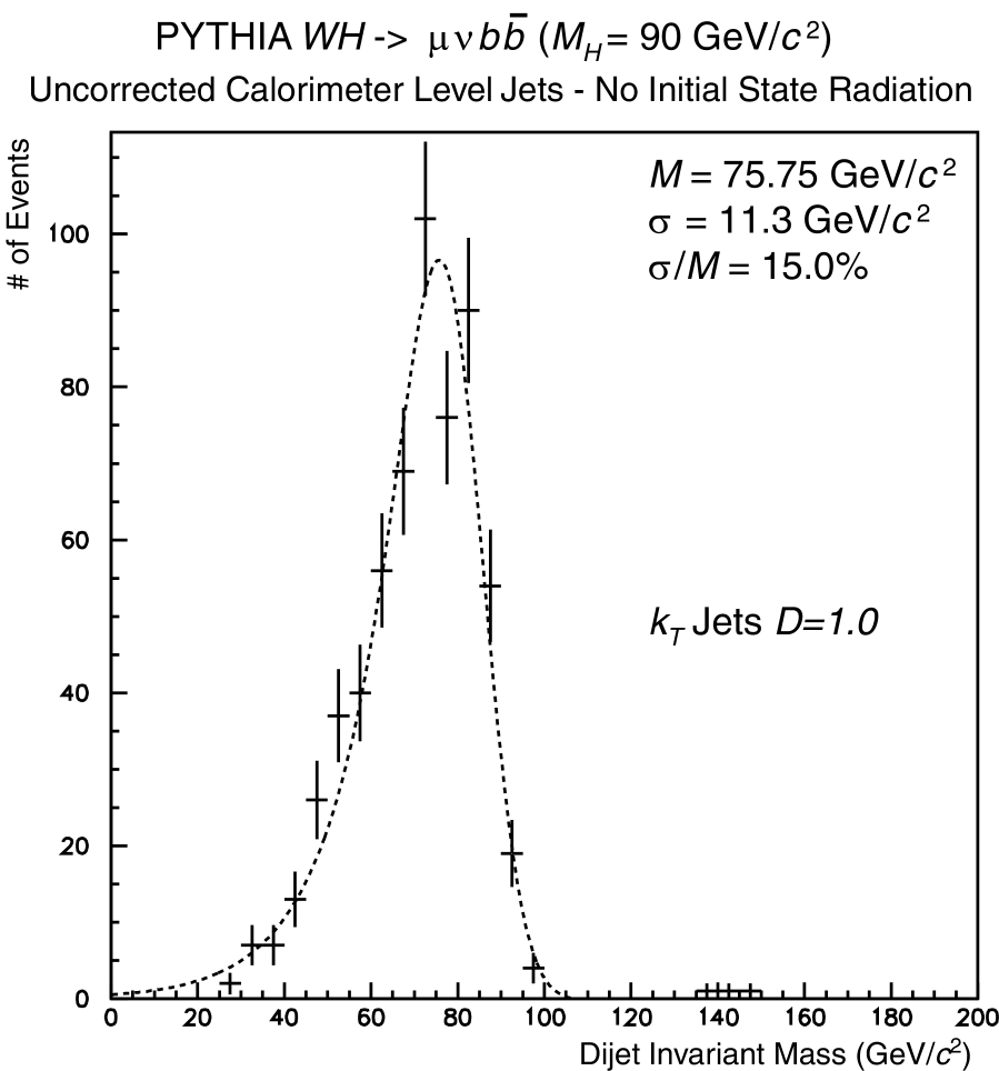
Comparison of Figure 31 with Figure 32(left), which was generated without final state radiation (FSR), shows that FSR contributes a low-end tail, because the jet algorithms fail to cluster in all the radiation. Initial State Radiation (ISR) on the other hand, contributes a high-end tail, because the jet algorithms cluster in extra (unwanted) radiation, as shown by Figure 32(right) which was generated without ISR. Comparison of the figures will also show that ISR and FSR bias the peak position by a few GeV as well as contributing to the resolution.
For , the ISR component of the mass resolution is roughly equivalent to the FSR piece; for , FSR contributes relatively more (giving a worse resolution overall). In principle, the parameter could be optimized to accept as much FSR as possible while rejecting ISR.
-quark matching \\
To simulate the effect of requiring a -tag within each of the jets used for the mass reconstruction, we required that the leading jets be the closest jets to the and parton directions. This significantly improves the resolution, because it cuts out events where one of the leading jets comes from FSR (and is hence likely to match a gluon rather than the or ). The improvement is seen both for cone jets and jets in Figure 33.
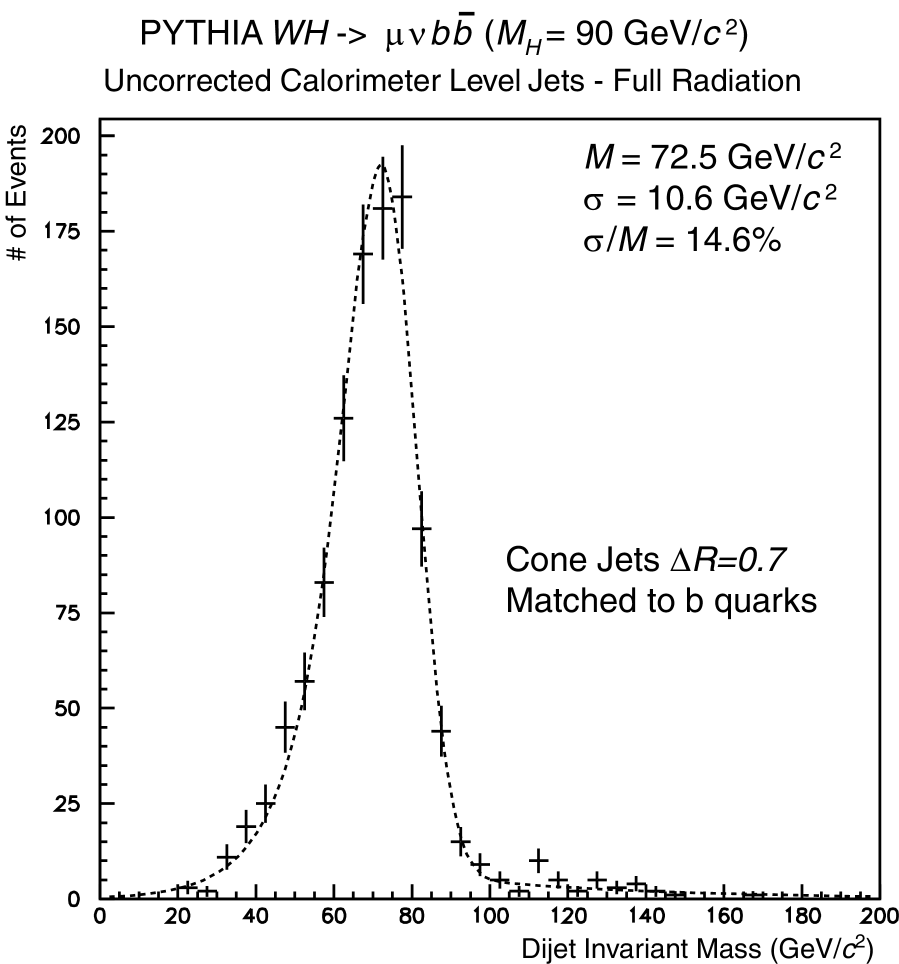
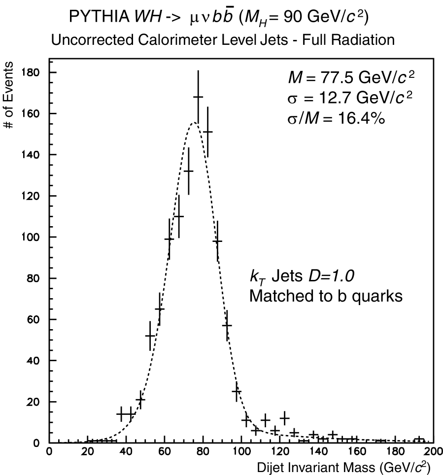
Luminosity Effects \\
We investigated the effects of multiple interactions per crossing on the dijet resolution. We overlaid real DØ zero-bias events from the highest luminosity phase of Run 1 on to our simulated Higgs events. A sample with instantaneous luminosity of cm-2s-1 was used, which has approximately 3.3 interactions per crossing on average. In Run 2b, with 100+ bunches and 132 ns between crossings, this is equivalent to cm-2s-1. The effect is shown in Figure 34 and, as can be seen, results in a significant worsening of the resolution. We have not attempted to recover the resolution but it might be possible to do better by imposing a threshold cut on calorimeter towers to remove some of the low-energy pileup.
We also investigated how the mass resolution is affected in overlaid events as a function of . Figure 35 shows the Higgs mass resolutions for both and . The smaller size exhibits less of a dependency on the luminosity. The algorithm’s parameter controls, approximately, the size of the jet, and smaller jet size will cover less calorimeter cells. Multiple interaction background can be approximated as a pedestal, distributed almost evenly in all towers of the calorimeter; so the smaller size parameter jets are affected less. The effects of multiple interactions have also been studies in the cone jet algorithms, as shown in Figure 36. The loss in resolution is similar for the algorithm.
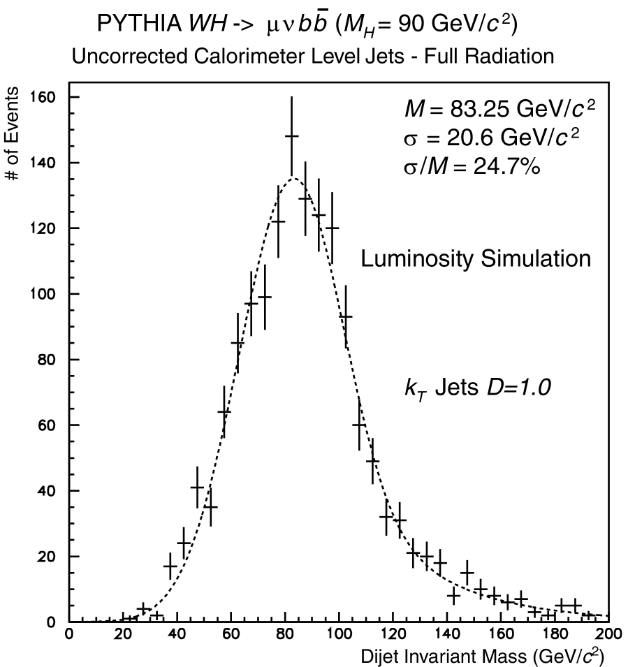
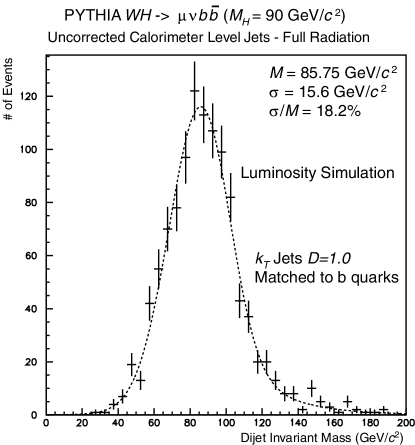
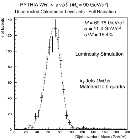
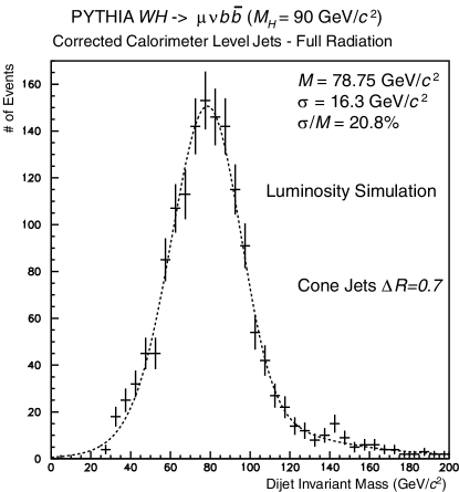
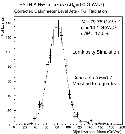
Conclusions \\
We have investigated many effects contributing to the invariant mass resolution. We find:
-
•
The algorithm is no silver bullet (at least as implemented in the DØ Run 1 software). In fact it is hard to do much better than a standard cone algorithm, especially if the jets are required to match the quark directions.
-
•
Jet energy corrections will have to be optimized for these relatively low- -quark jets.
-
•
Maintaining good resolution in the high luminosity environment of Run 2 and beyond will be a challenge. Pileup from minimum bias events can seriously degrade the energy resolution.
Table 3 summarizes the resolution and peak position of all the results.
| Cone | ||||||
|---|---|---|---|---|---|---|
| Data Sample | Peak | Width | Peak | Width | Peak | Width |
| (GeV/) | (GeV/) | (GeV/) | ||||
| Uncorr., no FSR | 80.2 | 15.3% | ||||
| Uncorr., no ISR | 75.7 | 15.0% | ||||
| Uncorr., full rad. | 72.5 | 14.6% | 73.7 | 20.1% | 67.25 | 22.7% |
| Uncorr., full rad., matching | 72.5 | 14.6% | 77.5 | 16.5% | ||
| Mult. int., uncorr., full rad. | 78.7 | 20.8% | 83.2 | 24.7% | ||
| Mult. int., uncorr., full rad., matching | 79.7 | 17.6% | 85.7 | 18.2% | 69.75 | 16.4% |
II.2.3 Study of -jet Tagging
M. Roco
To identify a jet associated with a quark, a technique, referred to as ’ tagging’, is performed by reconstructing the decay vertex of a long-lived hadron within the jet. The algorithm uses the precise track reconstruction of the silicon tracker to identify secondary vertices which are significantly displaced from the primary interaction vertex. The separation of a secondary vertex from the primary interaction vertex depends on the spatial resolution of the individual tracks associated to the secondary vertex and on the primary vertex resolution.
This report presents the results of a study performed to estimate the -tagging efficiency in and Higgs events by finding secondary vertices from -quark decays. The study is based on the MCFAST mcfast package, a useful tool designed to provide a fast simulation framework for detector design studies. It has been interfaced with either PYTHIA or ISAJET event generators for the parton fragmentation and hadronization. It performs parameterized tracking where for each generated track, a covariance matrix is assembled, which represents all the material and detector planes traversed by the ideal track. A reconstructed track is produced by smearing the generated track parameters according to this covariance matrix.
Detector Simulation \\
The implementation of the Run 2 DØ tracking detector geometry includes a solenoid which produces a 2 Tesla uniform magnetic field along the -axis. Within the magnetic field of the solenoid are the tracking detectors for charged particle identification. Drift chambers are used to simulate the scintillating central fiber tracker. A six barrel 4-layer geometry is used for the silicon microstrip tracker (SMT). For this study layers 1 and 3 of the four innermost barrels have 90o stereo angle.
The outermost barrels have single-sided detectors and therefore only give information. Layers 2 and 4 of all six barrels have 2o stereo. The barrel segments are separated by gaps containing F disks. The barrels are symmetric around and extend from cm to cm.
The beam vertex is centered at the origin with a smearing of 30 in both and and 25 cm in . In this study only one interaction per beam crossing is considered.
Tagging Algorithm \\
Given the relatively long lifetime of the quark, one can select jets arising from quark hadronization by ’tagging’ long-lived hadrons within jets. The decay of a long-lived hadron produces several charged tracks emanating from a point, or secondary vertex, separated from the primary interaction point.
Track displacement with respect to the primary vertex is measured using the perpendicular distance at the point of closest approach, or impact parameter shown in Fig. 37. The sign of is given by the location of the beamline in the transverse plane, relative to the particles’ trajectory in this plane. For positively charged tracks, the sign of is positive if the location of the beamline is outside the circle. The impact parameter resolution includes contributions coming from the intrinsic detector resolution, multiple scattering, and uncertainties from the primary vertex reconstruction. The impact parameter significance, , is a gaussian of width 1 with non-gaussian tails from heavy flavor quark content and and tracking errors. Fig. 38 shows the impact parameter and significance distributions for tracks originating from the primary vertex (top plots) and those tracks associated with the jets (bottom plots). Tracks from the hadron decays populate the tails of the distributions. Most particles in an event originate from the primary vertex.
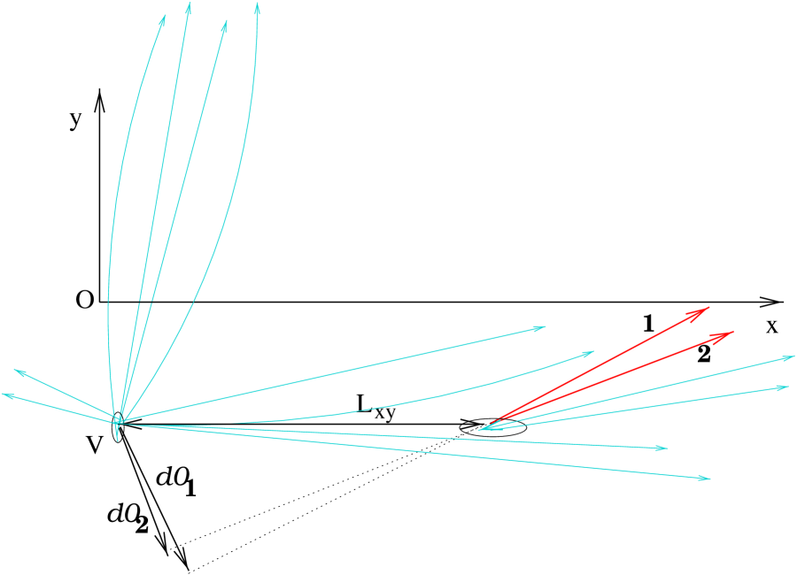
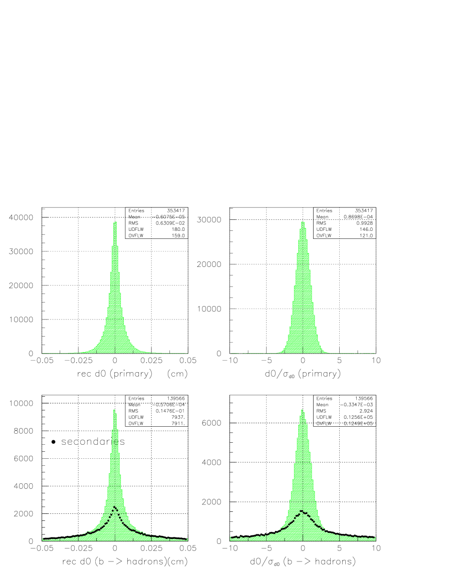
The algorithm loops over tracks associated to a jet of cone radius and 15 GeV/c. A tight selection criterion is applied in the first pass. If there are less than three tracks associated to the reconstructed decay vertex, a looser selection is applied. The selection is based on the track impact parameter significance. Fig. 39 shows the efficiency of the track selection using a sample of ISAJET events. It gives the fraction of jets, associated with either a or a hadron, which have at least three significantly displaced tracks (solid curves) for increasing cuts. The dashed curves show the corresponding efficiency if the requirement on the minimum number of tracks is relaxed to two. These plots show that a tight loose tagging scheme requiring at least two significantly displaced tracks keeps about 55% of the jets in the sample, while less than 5% of the jets associated with boson production (), mainly from charm hadron decays, are retained.
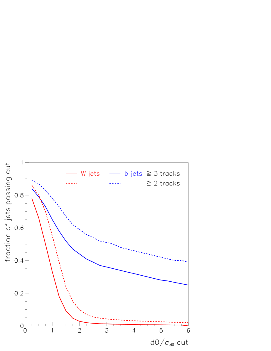
The selection criteria for the tight and loose algorithms, PASS1 and PASS2, are enumerated below:
-
PASS1 cuts:
-
-
track 0.5 GeV/c with at least 4 (axial + stereo) SMT hits
-
-
require cm to remove tracks consistent with conversions and and decays originating from the primary vertex
-
-
impact parameter significance,
-
-
give list of at least 3 candidate tracks to vertex finder
-
-
require at least 3 tracks associated to the vertex
-
-
-
PASS2 cuts:
-
-
track 1.5 GeV/c
-
-
impact parameter significance,
-
-
give list of at least 2 candidate tracks to vertex finder
-
-
require at least 2 tracks associated to the vertex
-
-
-
Secondary Vertex:
-
-
candidate tracks are passed to a 3D constrained vertex fit
-
-
find a set of pairwise compatible tracks and
-
-
reject tracks whose contribution to the overall of the fit 16
-
-
per degree of freedom of vertex fit
-
-
calculate the 2D decay length, , and its error
-
-
sign of = dot product of and the jet direction
-
-
require and cm
-
-
Candidate tracks are constrained to a common vertex to determine the transverse decay length . A vertex position is calculated and tracks with a large contribution to the overall fit are excluded. There should be at least two tracks used in the vertex fit. The reconstructed vertex is required to be within the innermost layer of the SMT, with 2.5 cm, and that the decay length significance be 3.
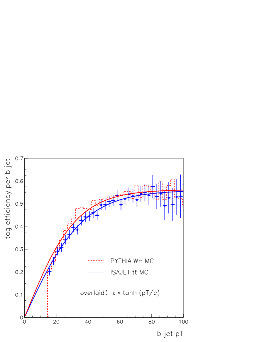
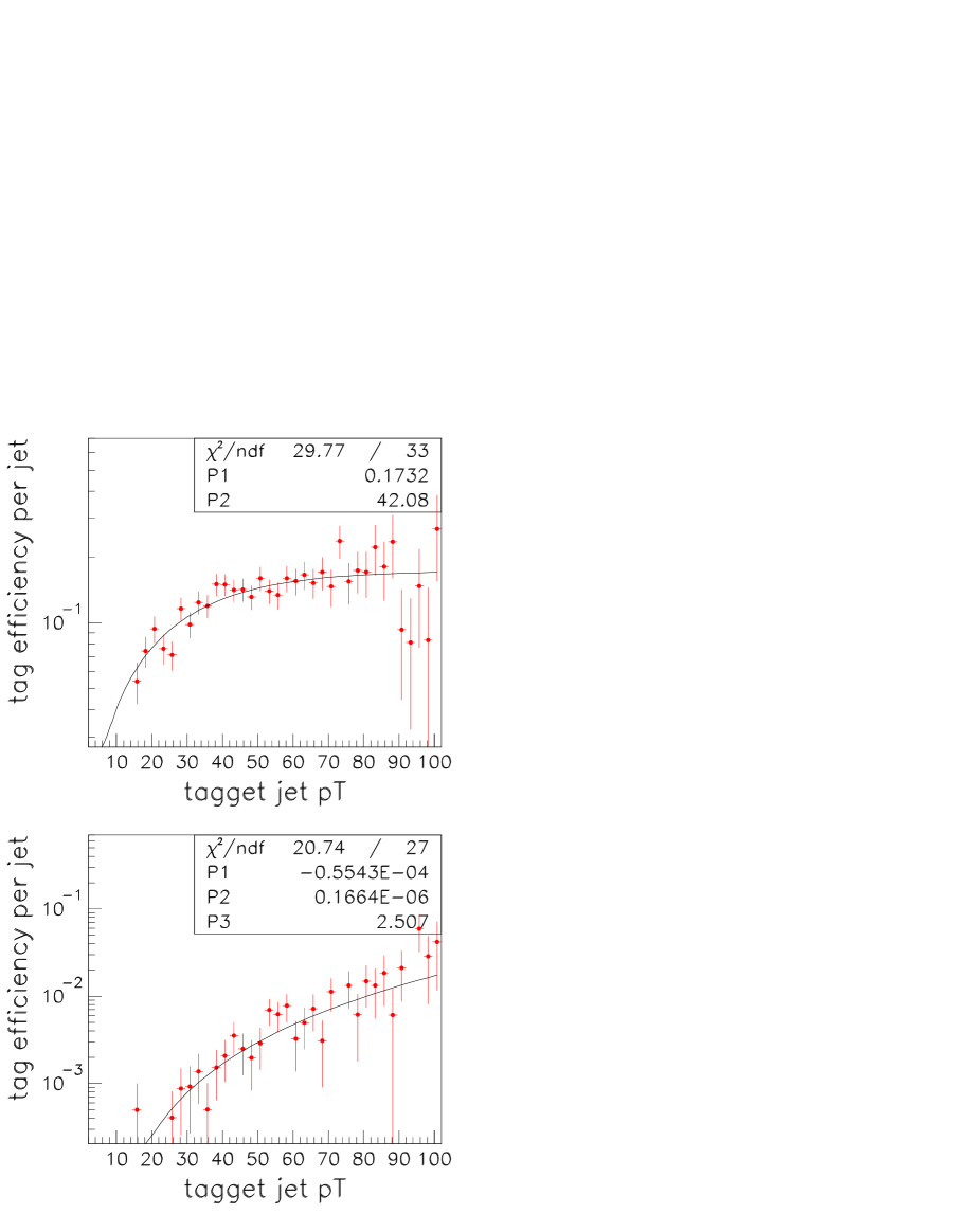
Tag Rates \\
The tag rates obtained after applying the selection criteria enumerated above are shown in Figs. 40 and 41. The plot in Fig. 40 shows a comparison of the -tag rates for two different samples, a sample generated using ISAJET shown as the points and a Higgs sample () generated using PYTHIA shown as the dashed histogram. The tag rates are parameterized in terms of the -jet using the functional form , where and are the constants obtained from the average of the two fits. This plot also shows that the difference between the rates obtained assuming different fragmentation and hadronization schemes is small.
Fig. 41 shows the efficiency of mistagging light quark or gluon jets as -jets. The tag rate for -jets, shown in the top plot, is roughly one third of the -jet tag rate. Tag rates for and jets, shown in the bottom plot, are less than 1% for GeV. However, this still presents a serious problem when dealing with background QCD multi-jet events with cross sections which are orders of magnitude larger than the or the expected Higgs production cross sections.
II.3 Low-mass Standard Model Higgs Bosons: 90–130 GeV
II.3.1 Channel
E. Barberis, W. Bokhari, P. Bhat, R. Gilmartin, H. Prosper, W. Yao\\
Previous studies tev2k ; snowmass96 ; tev33 have indicated that the channel, with and is the single most powerful channel to detect a Higgs signal over the large expected background. We present here three different analyses of this channel, each an extension of the previous. The initial analysis uses events produced by a well–established Run 1 CDF detector simulation, QFL′ and sequential selection requirements on a single variable at a time. The second analysis is similar to the first, but uses the SHW detector simulation developed for this workshop. The final analysis also uses SHW for detector simulation, but neural network techniques are employed to maximize the sensitivity. The good agreement between the first and second analyses indicates the quality of the SHW simulation, and the third analysis illustrates potential improvements to the sensitivity of this channel.
1a. , QFL′ Simulation and Traditional Techniques
This section presents study of production, where using a proven Run 1 CDF detector simulation for the signal and background estimation.
Event Samples \\
Throughout this section, we use Monte Carlo events generated with Pythia event generator and simulated with current CDF fast detector simulation, QFL′. This would allow us to have a realistic calorimeter simulation, and good central lepton identification (, and isolated tracks from decay). We do not attempt to simulate the leptons in the region ,282828This region was outside the Run 1 lepton acceptance, but it is being instrumented for Run 2. but rather, simply rescale the number of identified central leptons by the ratio of leptons between and at the generator level.
For the signal we generated 30K Pythia Monte Carlo events at each mass, in which the decays freely and Higgs is forced to decay into .
Background events come predominantly from the direct production of bosons in association with heavy quarks ( ), , single top production (, ) xsec and diboson . The requirement of two jets, along with the and isolated lepton requirements, remove essentially all generic multijet events.
To estimate the plus heavy quark backgrounds, we use the Herwig Monte Carlo program to calculate the fraction of +jet events that contain heavy quarks and the corresponding tagging efficiencies. The number of background events in a given jet multiplicity bin is then obtained as the product of heavy flavor fraction and tagging efficiency times the observed number of +jet events per 1 fb-1.
The top quark contributions ( and single top) are estimated using Pythia Monte Carlo and a theoretical calculation of pb, pb, and pb for a top quark mass of 175 GeV/.
The background is calculated using PYTHIA and a leading order cross section of 3.2 pb.
For the -tagging, we start with the jets observed in the calorimeter ( GeV and ) that are matched in a cone of to the quark at the four–vector level. The -tagging efficiency is parametrized as a function of jet using Run 1 data as described below.
-tagging Efficiency \\
The ability to tag jets with high efficiency and low mistagging rate is vital for searching for the decay of . The technique for -tagging has been well established in CDF using the Silicon Vertex tagger (SECVTX) and the Soft-Lepton Tagger (SLT), but will be much improved in the Run 2 Tevatron detectors cdfii ; d0upg . The full 3-D silicon tracker will eliminate a large fraction of mistags, allowing greater efficiency. The stand-alone pattern recognition in the silicon tracker (SVX-II and ISL) will allow tagging to extend into the region.
In this section, we use the same tag efficiencies and mistag rate per jet inside the SVX fiducial region measured in the CDF Run 1 data as in Figure 23.
The tight -tagger is the default CDF secondary vertex tagger (SECVTX). The loose -tagger includes the SLT tags with GeV and the jet-probability tags with a cut at 5%.
Trigger Requirements \\
The events are required to pass the following triggers:
-
•
High- inclusive lepton trigger ( GeV/c2 and ). (This selects , .)
-
•
GeV plus -tagging: Selects , and .
Selection Criteria \\
In order to reduce the large standard model backgrounds, we impose the following conventional selections based on the optimization of ratio, where S and B are the number of signal and the background events passing the selections.
-
•
Prompt isolated lepton with GeV/c.
-
•
Isolated tracks from decay also included ( GeV, GeV in cone ).
-
•
GeV.
-
•
Jet raw GeV, in cone
-
•
Two -tagged jets in GeV and , one tight SECVTX and other loose (SECVTX, JPB, SLT).
-
•
One jet raw GeV
-
•
No extra jet with GeV and .
-
•
Any events containing two isolated tracks ( GeV, ) are removed.
-
•
A requirement that the reconstructed mass of jet system be near the target Higgs mass. (Described below.)
Figure 42 shows the jet distributions for signal and backgrounds. We also considered requirements on the and the Higgs scattering angle in the rest frame, but these did not significantly improve the result.

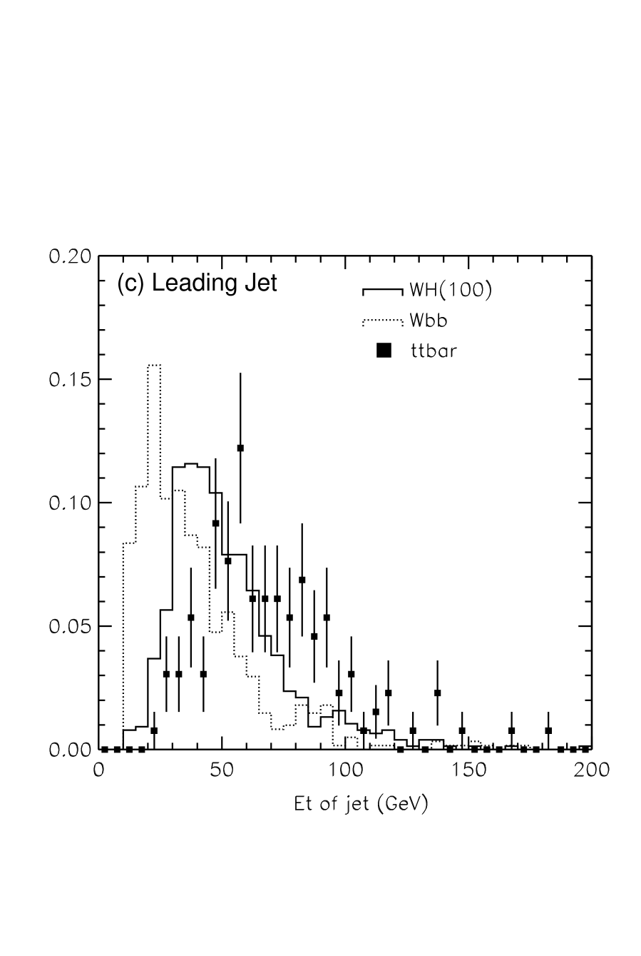
To increase the sensitivity of the search we look for a peak in the reconstructed two-jet invariant mass distribution using the 4-momenta of jets as measured by the calorimeter after correction for detector effects. With the present detector resolution, we found the dijet mass resolution GeV/c2 for the Higgs mass at 110 GeV/c2. The expected two-jet invariant mass distributions for , and are shown in Figure 43.

The studies described above in this report indicate that significant improvement in the dijet mass resolution (30%) is available if the jet reconstruction uses information from tracking and shower maximum detectors as well as the calorimeter energies used thus far. Such an improvement has been incorporated in this study by rescaling the default di-jet mass resolution down by 30%.
The mass windows we used to count for signal are listed in Table 4.
Results \\
The overall acceptance, including and dijet mass requirement, ranges from 2.0% to 2.3% and is shown in Table 4, for the Higgs mass between 90 to 130 GeV/c2. The numbers of expected events and the corresponding background estimates per 1 fb-1 are summarized in Table 4. The luminosity required for 95% CL exclusion and 5 discovery are shown in Figure 44.
| (GeV/c2) | 90 | 100 | 110 | 120 | 130 |
|---|---|---|---|---|---|
| (76.7,103.3) | (84.6,116.8) | (91.8,123.3) | (89.3,134.7) | (104.8,144.0) | |
| (pb) | 0.42 | 0.30 | 0.22 | 0.16 | 0.12 |
| B( | 2.0% | 2.2% | 2.3% | 2.3% | 1.9% |
| signal events | 8.4 | 6.6 | 5.0 | 3.7 | 2.2 |
| 21.5 | 20.6 | 18.9 | 19.7 | 15.4 | |
| 7.7 | 7.3 | 4.9 | 2.3 | 0.6 | |
| 9.6 | 12.3 | 12.2 | 13.8 | 13.0 | |
| 6.7 | 8.5 | 8.4 | 9.6 | 9.1 | |
| 2.7 | 3.5 | 3.4 | 3.9 | 3.6 | |
| background | 48.2 | 52.2 | 47.8 | 49.3 | 41.7 |
| 1.2 | 0.91 | 0.72 | 0.53 | 0.34 |

1b. , SHW Simulation and Traditional Techniques
The present study differs from the previous studies primarily in that it uses more detailed Run 2 simulation of detector efficiencies and resolutions, carried out by the SHW simulation package. The analysis uses Monte Carlo generated event samples for the signal and all backgrounds. Cross section estimates are taken either from data measurements (such as the cross section) or from theoretical predictions including highest order corrections to the particular process. Trigger efficiencies are assumed to be for this channel, physics object reconstruction (leptons, jets, ) is done by SHW. The efficiency for tagging jets is parametrized according to the efficiency measured by the CDF Run 1 detector, and cross-checked with the result of a simulation of the Run 2 DØ Microstrip Silicon Tracker.292929See Section II.B.3. The event shapes for signal and background were carefully studied to determine the selection which maximizes significance, given in the gaussian regime as . A significance value is calculated for fixed Higgs masses and different values of the di-jet (i.e. ) mass resolution, as a function of luminosity.
Event samples \\
The background processes to the channel are , , , single top production and QCD. The requirement of double tagging reduces the contribution of processes containing mostly light quark jets, such as QCD and other than . These processes will not be considered any further. Single top consists of Drell-Yan (- in the final state) and -gluon fusion (-light quark- in the final state) processes. A small contribution comes also from -light quark final states, which are simulated as well. The PYTHIA generator PYTHIA is used to simulate (for values of the Higgs mass of 80, 90, 100, 110, 120, and 130 GeV/), , , and single top events; is generated using the CompHEP package comphep . Cross section values for the different processes are listed in Table 5.
| (pb) | 3.2 | 10.6303030this is the result of multiplying the CompHep cross section by approximately a factor 1.4, as suggested by a conversation with K. Ellis | 7.5 | 2.4 | 1.0 |
Although we are not directly considering reconstructed ’s, decays into are simulated, since the can feed into the signal and background samples via the and decay modes. Detector simulation for all samples was performed using standard SHW.
Selection Criteria \\
The following selection criteria are applied:
-
•
One and only one isolated lepton (either or ), veto on additional leptons with GeV.
-
•
primary lepton GeV.
-
•
GeV
-
•
Jet veto cuts:
-
-
No extra jets with and .
-
-
extra jet with and .
-
-
-
•
cut on
The double tagging requirement consists of:
-
•
One tight tag, with efficiency parameterized, as a function of , by: 0.57(tanh(()/26.5)).
-
•
One loose tag, with efficiency of a tight tag, enhanced by a factor: 0.35(tanh(/26.5).
-
•
tagged jets GeV and .
The tagging efficiencies are obtained from fits to CDF Run 1 data, and are in good agreement with the results of a MCFAST simulation of the Run 2 detector, under similar assumptions for the tagging algorithms. Both efficiencies are rescaled by a factor 1.1 to take into account soft lepton tagging. The total double tag efficiency is in the range . Corrections are applied to relate the energy of jets and untagged jets to the initial parton energies, before QCD radiation. The sequential effect of the cuts on the event samples is shown in Table 6.
| (110 GeV) | ||||||
|---|---|---|---|---|---|---|
| Generated | 5000 | 80000 | 5000 | 45000 | 7000 | 6227 |
| One lepton (veto secondary leptons) | 2663 | 38736 | 2408 | 16149 | 3657 | 1651 |
| lepton | 1981 | 29072 | 1694 | 9761 | 2839 | 847 |
| 1763 | 22880 | 1437 | 8967 | 2558 | 779 | |
| double tag | 666 | 4512 | 497 | 4160 | 236 | 324 |
| jet vetoes | 382 | 4432 | 322 | 328 | 55 | 141 |
| cut () | 345 | 1248 | 271 | 130 | 6 | 65 |
The mass resolution of the system, after all corrections are applied to the SHW jets, is approximately 15%, and the distribution itself is shown if Figure 45. Since it is foreseen in Run II to achieve better values in dijet mass resolution, the resolution here is assumed as a free parameter and the analysis is performed for a set of different hypotheses. The effect of the resolution on the significance for a 100 GeV Higgs signal in 10 fb-1 is illustrated in Figure 46.

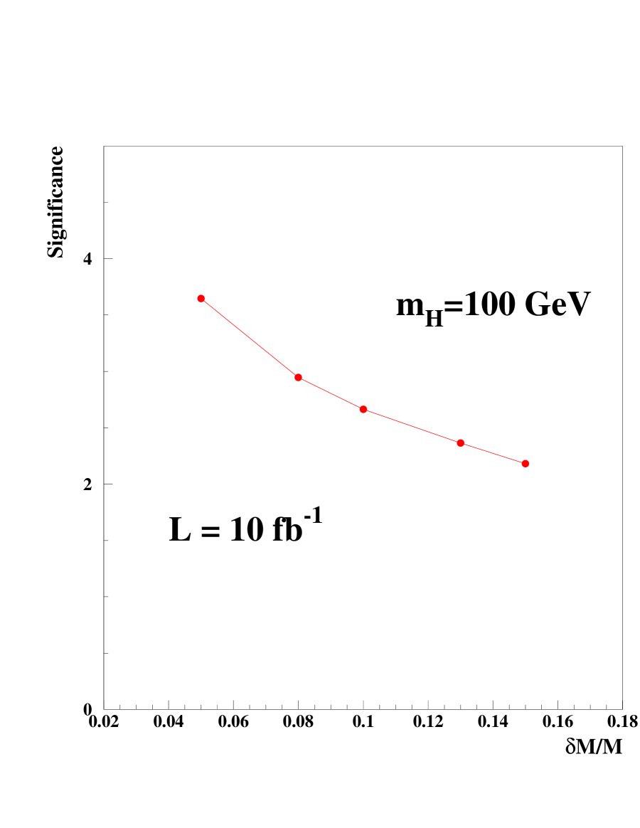
Results and Conclusions \\
The number of signal and background events after all selection cuts are applied is listed in Tables 7, 8 and 9 for three values of mass resolution and for 1 fb-1 of data. The significance values for each Higgs mass and mass resolution are listed in Table 10. Figure 47 shows the significance values scaled to 10 fb-1 as a function of Higgs mass for the different mass resolutions.
The luminosity required to observe a Higgs signal in the channel at different confidence levels is shown in Figure 48. The channel appears to be the most significant for Higgs masses below 130 GeV/.
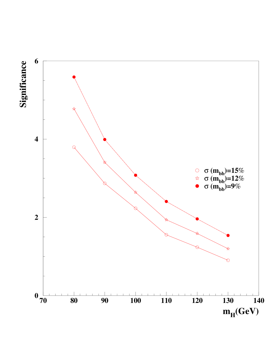
| (GeV/) | 80 | 90 | 100 | 110 | 120 | 130 |
|---|---|---|---|---|---|---|
| signal events (S) | 14 | 10 | 8 | 5 | 4 | 3 |
| 94 | 76 | 68 | 63 | 59 | 59 | |
| 10 | 11 | 11 | 11 | 11 | 10 | |
| 22 | 23 | 26 | 30 | 34 | 37 | |
| single top | 92 | 11 | 11 | 12 | 14 | 15 |
| total background (B) | 136 | 121 | 117 | 117 | 119 | 122 |
| (GeV/) | 80 | 90 | 100 | 110 | 120 | 130 |
|---|---|---|---|---|---|---|
| signal events (S) | 14 | 10 | 8 | 5 | 4 | 3 |
| 59 | 54 | 47 | 38 | 32 | 28 | |
| 8.6 | 10 | 8.8 | 7.2 | 6.0 | 4.4 | |
| 12 | 16 | 19 | 21 | 24 | 26 | |
| single top | 5.1 | 6.0 | 8.4 | 9.2 | 10 | 11 |
| total background (B) | 85 | 86 | 84 | 75 | 72 | 70 |
| 1.5 | 1.1 | 0.9 | 0.6 | 0.5 | 0.4 |
| (GeV/) | 80 | 90 | 100 | 110 | 120 | 130 |
| signal events(S) | 14 | 10 | 8 | 5 | 4 | 3 |
| 50 | 45 | 36 | 29 | 25 | 19 | |
| 7 | 10 | 9 | 6 | 4 | 2 | |
| 9 | 14 | 16 | 15 | 20 | 22 | |
| single top | 3 | 6 | 7 | 7 | 9 | 9 |
| total background (B) | 69 | 75 | 68 | 57 | 58 | 52 |
| 1.7 | 1.2 | 0.9 | 0.7 | 0.6 | 0.4 |
| (GeV/) | 80 | 90 | 100 | 110 | 120 | 130 |
|---|---|---|---|---|---|---|
| : | ||||||
| ( | 1.2 | 0.9 | 0.7 | 0.5 | 0.4 | 0.3 |
| ( | 1.5 | 1.1 | 0.8 | 0.6 | 0.5 | 0.4 |
| ( | 1.7 | 1.2 | 0.9 | 0.7 | 0.6 | 0.4 |
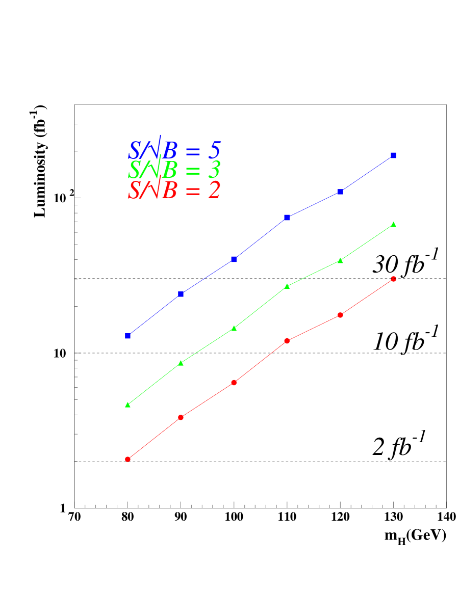
1c. , SHW Simulation and Neural Network Techniques
Optimal Event Selection \\
Given any set of variables, it is useful to construct the discriminant function , given by
where is the vector of variables and and , respectively, are the dimensional probability densities describing the signal and background prosper_bhat . A cut on the single variable yields the optimal demarcation between signal and background. The variable is related to the Bayes discriminant function, which is proportional to the likelihood ratio . The discrimination is optimal in the sense that it minimizes the probability to mis-classify events.
Of the several methods available to approximate the discriminant , neural networks are the most convenient because they approximate directly blum . To compute , we have used the JETNET package jetnet to train three-layer (that is, input, hidden and output) feed-forward networks. The training was done using the backpropagation algorithm, with the desired output for the signal set to one and that for the background set to zero.
Event Samples \\
We have considered final states with a high electron (e) or muon () and a neutrino from decay and two quarks () from Higgs decay. The events were generated using the PYTHIA program (version 6.023) for Higgs masses of = 80, 90, 100, 110, 120, 130 and 140 GeV/c2. The cross section times branching ratio (BR) for the process where , are listed in Table 11.
| (GeV/c2) | |
|---|---|
| 80 | 0.17 |
| 90 | 0.119 |
| 100 | 0.085 |
| 110 | 0.062 |
| 120 | 0.045 |
| 130 | 0.034 |
| 140 | 0.011 |
| Backgrounds | |
| 3.5 | |
| 0.165 | |
| 0.8 | |
| (pb) | |
| 1.0 | |
| 7.5 |
The background processes which are important for this search are , , and single top production (, ). They have the same signature, , as the signal. The sample was generated using CompHEP, a parton level Monte Carlo program based on exact leading order (LO) matrix elements, with the fragmentation of partons done using PYTHIA. The single top, and events were generated using PYTHIA. The (s-channel) process was generated using off-shell production, with , and selecting the final state. In Table 11 , we list the cross sections we have used for the background processes.
The SHW program was used for detector simulation. It provides a fast (approximate) simulation of the trigger, tracks, calorimeter clustering, event reconstruction and c and b-tagging. The SHW simulation predicts a di-jet mass resolution of about 14% at = 100 GeV/, varying only slightly over the mass range of interest. However, to allow for comparisons with the other and studies, we have rescaled the di-jet mass variables for all signal and background events so that the resolution is 10% at each Higgs boson mass.
Selection Criteria \\
We applied the following requirements to produce a base sample to which the neural network was then applied:
-
•
the transverse momentum of the isolated lepton GeV,
-
•
the pseudorapidity of the lepton ,
-
•
the missing transverse energy in the event GeV,
-
•
two or more jets in the event with GeV and .
In order to reduce the dominant background, we assumed that the two jets will be -tagged. We then searched for variables that discriminate between the signal and the backgrounds and arrived at the following set:
-
•
of the -tagged jets
-
•
– invariant mass of the -tagged jets
-
•
– sum of the transverse energy of all selected jets
-
•
of the lepton
-
•
of the lepton
-
•
– missing tranverse energy
-
•
– sphericity
-
•
between the -tagged jets
-
•
between the lepton and first -tagged jet
-
•
between the lepton and second -tagged jet
| GeV/c2 | 80 | 90 | 100 | 110 | 120 | 130 | 140 |
|---|---|---|---|---|---|---|---|
| Number of events | |||||||
| 12.71 | 8.65 | 8.97 | 4.81 | 4.41 | 3.71 | 1.22 | |
| 17.51 | 12.28 | 12.48 | 5.84 | 9.66 | 20.12 | 10.26 | |
| 6.89 | 7.52 | 10.32 | 1.72 | 1.00 | 0.97 | 0.18 | |
| 0.55 | 0.51 | 0.95 | 0.58 | 0.71 | 0.96 | 0.91 | |
| 2.95 | 2.46 | 5.40 | 3.44 | 5.89 | 9.33 | 8.35 | |
| 3.34 | 5.63 | 9.89 | 7.24 | 8.39 | 14.49 | 14.15 | |
| Total background | 31.23 | 28.40 | 39.04 | 18.81 | 25.67 | 45.87 | 33.84 |
The networks were configured with 7 input variables, 9 hidden nodes and one output node. The subset of variables used to train the networks, one network for each Higgs mass and for each of the three dominant backgrounds, are listed in Table 12. We show the distributions of some of these variables for and in Figures 49 and 50.
Figure 51 shows the distributions of network output for each background relative to the signal with GeV/c2. We see that all backgrounds, with the exception of , are well separated from the signal. For Higgs masses close to the mass the background is kinematically identical to the signal and therefore difficult to deal with. But for Higgs masses well above the mass the discrimination between and improves, as does that between and the other backgrounds.
The final selection is a requirement that the neural network output , which is defined to the range , satisfy in which is a Higgs–mass dependent value. The final numbers of expected signal and background events are given in Table 13.
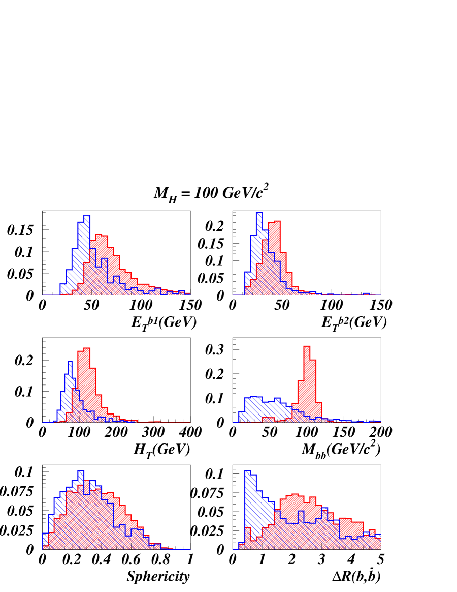
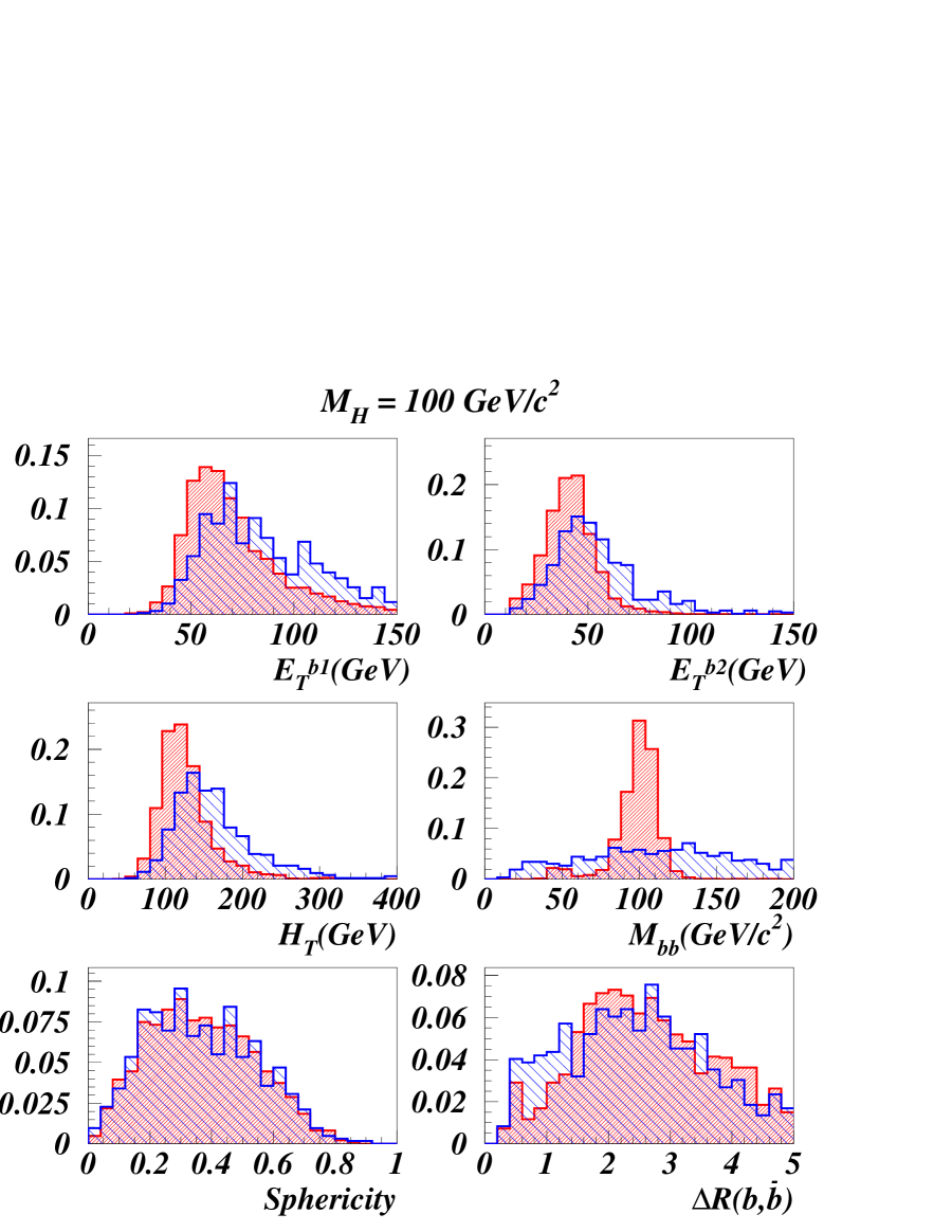
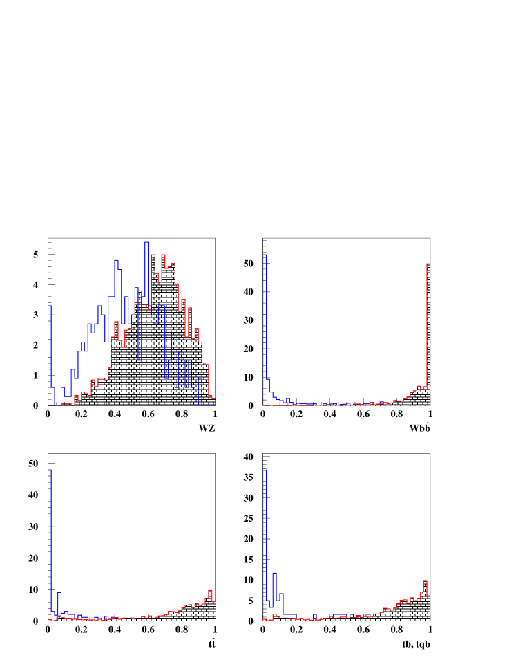
II.3.2 Channel
P. Bhat, W. Bokhari, J. Conway, R. Demina, R. Gilmartin, D. Hedin, R. Jesik, M. Kruse, H. Prosper, V. Sirotenko, W. Yao \\
The cross section times branching ratio for the mode is comparable to that for the mode discussed in the previous section. If the backgrounds at fixed efficiency were similar, the channel would have as much sensitivity as previous. Three analyses of this final state are presented here. The first is an analysis based on the CDF Run 1 result, using the QFL′ simulation. The second is an analysis selection developed using SHW simulated events. The third analysis of this section is an extension of the SHW analysis applying neural network techniques to the event selection.
2a. , QFL′ Simulation and Traditional Techniques
We have repeated the study of reported at Snowmass 96 snowmass96 using QFL′ and found consistent results. This analysis achieves sensitivity via a tight selection which reduces the background to a low level.
Event Samples\\
The event samples used in this analysis were produced as described in the section for the QFL′ analysis.
Selection Criteria\\
For the , We apply the following kinematic selection criteria:
-
•
Raw GeV to pass the trigger requirement.
-
•
Two tagged jets with GeV in .
-
•
Minimum between and any jets GeV and .
-
•
No extra jet GeV in .
-
•
No isolated track above 10 GeV in the events, where the isolation requirement is GeV over the additional tracks inside the cone .
The numbers of observed events and the corresponding background estimates for 1 fb-1 at TeV, are summarized in Table 14. As in the channel, the backgrounds are dominated by vector boson and top quark production. Generic multijet events are removed very efficiently by the requirements of two jets and large missing . This background is extremely difficult and unreliable to simulate due to the large cross section and very small acceptance, and must be estimated with real data. In the CDF Run 1 Higgs search, the dijet background was about half of the total. With tighter selection criteria, such as a back-to-back cut on the jet azimuth, the authors believe that this background will represent no more than 50% of the total without loss of signal sensitivity.
| (GeV/c2) | 90 | 100 | 110 | 120 | 130 |
|---|---|---|---|---|---|
| (pb) | 0.24 | 0.18 | 0.13 | 0.1 | 0.074 |
| () | 1.5 | 1.7 | 2.1 | 1.7 | 1.2 |
| signal (S) | 3.6 | 3.1 | 2.7 | 1.7 | 0.9 |
| backgrounds | |||||
| , | 6.53 | 5.20 | 4.9 | 4.83 | 3.77 |
| 5.43 | 4.90 | 3.4 | 1.33 | 0.0 | |
| top | 1.63 | 2.2 | 2.2 | 2.2 | 2.2 |
| backgrounda (B) | 13.6 | 12.3 | 10.4 | 8.3 | 5.9 |
aThis does not include dijet production processes, which must be estimated from data; see text.\\
2b. , SHW Simulation and Traditional Techniques
In the previous analysis, hard cuts on raw missing transverse energy and additional jet activity were used reduce the background to an acceptable level. For the analysis presented here, a different strategy is used in which a looser selection gives both larger signal and larger background but with approximately the same statistical power as the previous analysis.
Event samples \\
The signature of decays is two -jets with large invariant mass and either large missing energy (), or two opposite sign leptons with mass near that of the . These requirements effectively eliminate generic multijet events, as shown below, and leave the following background processes: , , , and single top production. The selection also picks up events with decay, particularly if the leptons escape detection. This introduces additional backgrounds from and processes and adds events to the effective signal. and events are generated using PYTHIA (for Higgs mass values of 90, 100, 110, 120, and 130 GeV). PYTHIA is also used for the , , , and single backgrounds, and CompHEP is used for and . The simulation is checked against ISAJET, and the results agree to within 8%. Cross sections and branching ratios for both the signal and background processes are taken directly from the generators without any correction factors applied, except for events which are normalized to the measured cross section. Detector simulation for all samples is performed using the SHW package.
As in the previous analysis, no estimate for the level of background from dijet production is made here, as it will require actual data.
Selection Criteria \\
events are selected by the following criteria:
-
•
2 -jets:
-
-
one tight -tagged jet with GeV and
-
-
one loose -tagged jet with GeV and
-
-
-
•
missing transverse energy GeV
-
•
the angle between the and its closest jet
-
•
reject events with one or more isolated leptons with ( GeV/c)
-
•
scalar sum of hadronic energy GeV
The -tagging and lepton identification efficiencies are all taken from SHW. The effect of the cuts on both the 100 GeV Higgs signal and background samples is shown in Table 15. As shown in Figure 52, the cut removes generic multijet background, and the additional cut on removes multijet events with due to mismeasured jets. Combined with the requirement of two -tagged jets, few generic multijet events remain; based on Run 1 data, we believe that the background from multijet events will be no more than 50% of the total background from all sources. The isolated lepton cuts reduce the backgrounds involving decay. However, significant contributions remain due to muon detection inefficiencies (which also add to the apparent of an event). This also means that events contribute to the effective signal.
It should be noted that the search mode selection requires the detection of a high lepton, so the two samples are independent. The cut helps remove background (see Figure 52), and cuts much less of the signal than the third jet veto used to veto top in previous analyses (increasing the significance by as much as 30%). Energy corrections are applied to the -jets to correct for final state radiation and undetected energy from semileptonic decays. Only the two highest -jets in an event are used as the candidate jets from the Higgs decay.
| channel | |||||||||
|---|---|---|---|---|---|---|---|---|---|
| (fb) | 27.0 | 71.5 | 137 | 135 | 668 | 2530 | 6800 | 1000 | 807 |
| generated | 7000 | 7000 | 7000 | 7000 | 20000 | 20000 | 270000 | 6223 | 55000 |
| 2 -jets | 3022 | 2798 | 2437 | 2254 | 3694 | 3802 | 119713 | 2012 | 5036 |
| GeV | 2177 | 1744 | 941 | 1297 | 2573 | 1924 | 55559 | 555 | 3686 |
| 1983 | 1538 | 840 | 1171 | 2330 | 1704 | 48657 | 491 | 3324 | |
| GeV | 1527 | 831 | 668 | 802 | 1592 | 1526 | 2004 | 200 | 1660 |
| no isolated leptons | 1376 | 364 | 609 | 401 | 1458 | 680 | 767 | 99 | 902 |
| 1014 | 271 | 412 | 268 | 314 | 96 | 286 | 32 | 194 |
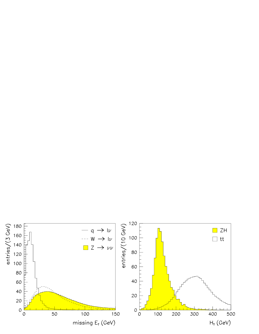
Results and Conclusions \\
Signal mass windows for each Higgs mass are determined using the nominal mass resolution obtained from SHW with -jet corrections ( for 100 GeV Higgs). The number of signal and background events expected in 1 fb-1 of data is shown in Table 16. Numbers obtained assuming a 10% mass resolution are also shown in the table. These results assume a 100% trigger efficiency. Efficiencies close to this should be obtainable with a multijet- trigger with the threshold set as low as the rates will allow. The addition of secondary vertex tagging at the trigger level would help keep the rates down if necessary, as would a veto on back–to–back jets.
| (GeV) | 90 | 100 | 110 | 120 | 130 |
|---|---|---|---|---|---|
| 70–110 | 80–125 | 85–130 | 90–140 | 95–150 | |
| (80–105) | (90–120) | (95–125) | (105–135) | (115–145) | |
| 4.9 | 3.9 | 2.8 | 1.9 | 1.3 | |
| 4.0 | 2.9 | 1.8 | 1.3 | 0.8 | |
| signal | 8.9 | 6.7 | 4.6 | 3.2 | 2.1 |
| 8.5 (8.5) | 8.0 (6.0) | 7.1 (2.9) | 5.8 (0.2) | 4.4 (0.0) | |
| 6.0 (5.9) | 5.9 (5.1) | 5.4 (2.7) | 4.7 (0.2) | 3.6 (0.0) | |
| 12.3 (7.0) | 10.3 (6.3) | 9.2 (5.6) | 8.7 (4.6) | 8.1 (3.5) | |
| 15.1 (8.5) | 12.1 (7.1) | 11.1 (6.7) | 10.5 (5.4) | 10.1 (4.2) | |
| single | 7.4 (4.6) | 8.0 (5.4) | 7.8 (5.3) | 8.0 (4.7) | 7.9 (3.8) |
| 6.3 (4.0) | 7.2 (4.7) | 7.0 (4.7) | 7.3 (4.3) | 7.2 (3.5) | |
| backgrounda | 55.6 (38.5) | 51.5 (34.6) | 47.6 (27.9) | 45.0 (19.4) | 41.3 (15.0) |
aThis does not include generic dijet production processes, which must be estimated from data; see text.\\
2c. , SHW Simulation and Neural Network Techniques
This section describes a neural network analysis applied to the final state. The technique is identical to that for the neural network analysis for the section.
Event Samples \\
The events were generated using PYTHIA for Higgs masses of 90, 100, 110, 120 and 130 GeV/c2. The principal backgrounds to production are , , single top and . The background sample was generated using CompHEP, with fragmentation done using PYTHIA, while all other samples were generated using PYTHIA. We used SHW to simulate the detector response and, as in the study, we assumed that two jets are -tagged. The cross sections for signal and background are shown in Table 17. As in the other two analyses, no dijet background is considered.
| (GeV/c2) | |
|---|---|
| 90 | 0.041 |
| 100 | 0.030 |
| 110 | 0.022 |
| 120 | 0.016 |
| 130 | 0.013 |
| Backgrounds | |
| 0.700 | |
| 0.800 | |
| (pb) | |
| 1.235 | |
| 1.000 | |
| 7.500 |
Selection Criteria \\
We applied the following requirements to produce a base sample to which the neural network was then applied:
-
•
the missing transverse momentum GeV
-
•
two or more jets in the event with GeV and
In order to reduce the dominant background, we assumed that the two jets will be -tagged.
A network was trained for each Higgs mass and for each of the backgrounds with the following variables
-
•
of the -tagged jets
-
•
– invariant mass of the -tagged jets
-
•
– sum of jet transverse energies
-
•
-
•
– sphericity
-
•
Centrality ()
-
•
-
•
Minimum (jet,)
Results and Conclusions \\
Figure 53 shows the network output distributions , respectively. From these figures it is clear that discriminating between and its principal backgrounds is much more difficult than for and that further study is needed to identify better variables. Nonetheless, the channel contributes usefully to the final result. The results for the channel are in Table 18.
| (GeV/c2) | 90 | 100 | 110 | 120 | 130 |
|---|---|---|---|---|---|
| number of events | |||||
| 6.66 | 4.37 | 3.53 | 2.76 | 2.16 | |
| 5.59 | 3.75 | 2.79 | 1.98 | 1.70 | |
| signal | 12.25 | 8.12 | 6.32 | 4.74 | 3.86 |
| 8.12 | 4.97 | 4.83 | 3.85 | 3.92 | |
| 21.70 | 13.12 | 10.68 | 8.22 | 7.53 | |
| 11.24 | 6.14 | 2.59 | 1.05 | 0.59 | |
| 7.95 | 4.49 | 1.99 | 0.90 | 0.54 | |
| 0.63 | 0.27 | 0.37 | 0.24 | 0.29 | |
| 6.83 | 2.99 | 4.27 | 5.12 | 6.40 | |
| 5.10 | 2.70 | 3.00 | 3.00 | 4.35 | |
| backgrounda | 61.57 | 34.80 | 27.73 | 22.38 | 23.62 |
aThis does not include generic dijet production processes, which must be estimated from data; see text.\\
.9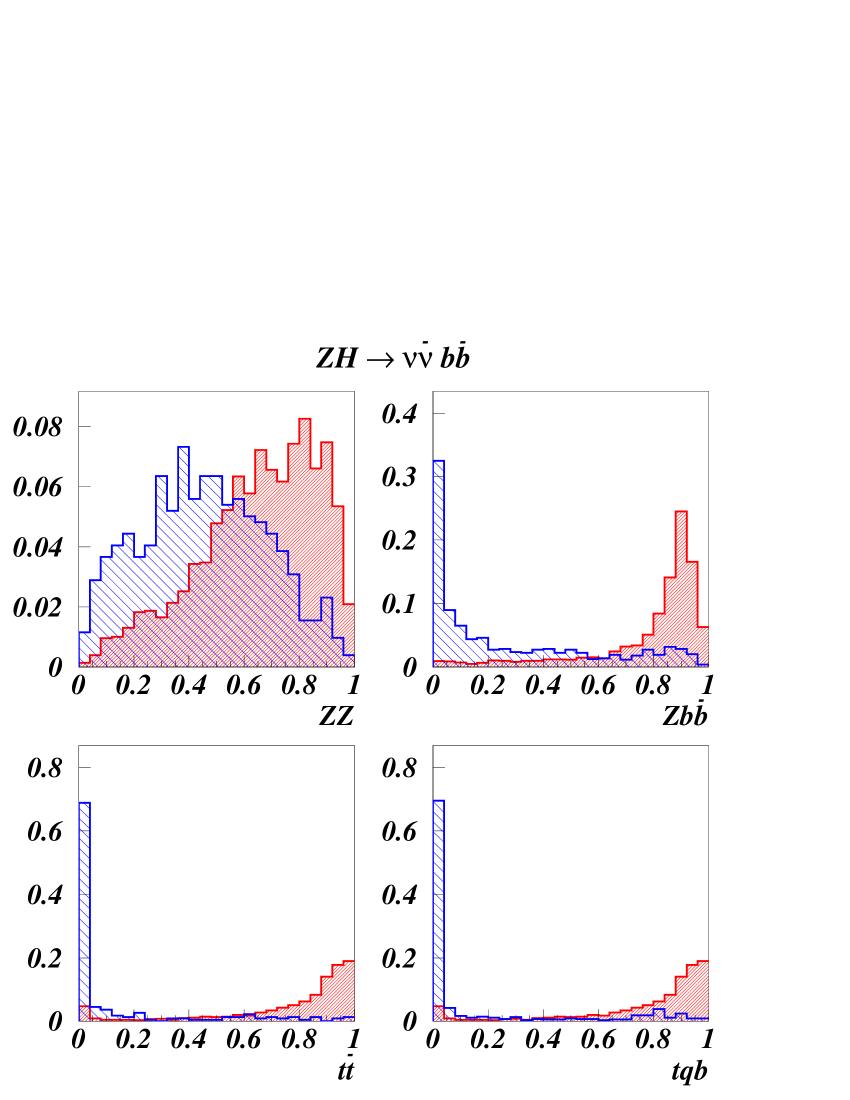
II.3.3 Channel
P. Bhat, R. Gilmartin, R. Jesik, M. Kruse, H. Prosper, W. Yao \\
Although the cross section times branching ratio for the final is roughly 1/3 that of the previous two channels, these events are easily and cleanly identified. Furthermore, given the high luminosity required for observation in the higher rate and channels, it is clear that every possible event is valuable to the Higgs search.
3a. , QFL′ Simulation and Traditional Techniques
The selection criteria for this channel are: In the channel, we select the dilepton events with the following cuts.
-
•
First lepton GeV,
-
•
Second lepton GeV,
-
•
GeV
-
•
Two -tagged jets with GeV and
The results are included with those for the channel described in section 2a.
1b. , SHW Simulation and Traditional Techniques
Event Samples\\
The event samples used in this SHW–based analysis were generated simultaneously with the samples used in the SHW–based analysis described previously.
Event Selection \\
events are selected by the following criteria:
-
•
2 -jets:
-
-
one tight -tagged jet with GeV and
-
-
one loose -tagged jet with GeV and
-
-
-
•
at least two opposite sign leptons ( or ) of the same flavor, \\ (tau’s are not explicitly searched for, but they contribute to the analysis)
-
•
both leptons with GeV/c
-
•
dilepton mass within 10 GeV/c2 of the mass
-
•
scalar sum of hadronic energy GeV
| (GeV/) | 90 | 100 | 110 | 120 | 130 |
|---|---|---|---|---|---|
| 70–110 | 80–125 | 85–130 | 90–140 | 95–150 | |
| (80–105) | (90–120) | (95–125) | (105–135) | (115–145) | |
| signal | 1.5 | 1.2 | 0.9 | 0.6 | 0.4 |
| 2.2 (2.2) | 2.1 (1.6) | 1.9 (0.8) | 1.5 (0.1) | 1.2 (0.0) | |
| 2.9 (1.6) | 2.4 (1.4) | 2.1 (1.2) | 2.0 (1.0) | 1.9 (0.8) | |
| 1.8 (1.1) | 1.9 (1.3) | 1.8 (1.2) | 1.9 (1.2) | 1.9 (1.1) | |
| background | 6.9 (4.9) | 6.4 (4.3) | 5.8 (3.2) | 5.4 (2.3) | 5.0 (1.9) |
| 0.57 (0.7) | 0.47 (0.6) | 0.37 (0.5) | 0.26 (0.4) | 0.18 (0.3) |
Results and Conclusions \\
The event flow through these cuts is similar to that in the analysis, except that there are no backgrounds involving the in this case. The two leptons in these events provide an easy, high efficiency trigger. The number of signal and background events expected in 1 fb-1, assuming a 100% efficient trigger is shown in Table 19. These events are independent of both the and samples.
Combining both the and channels, a three sigma observation of a 100 GeV/ Higgs would require 8 fb-1 for a single experiment. If a 30% improvement in mass resolution with respect to that of Run 1 can be achieved, only 5 fb-1 would be required. The mass distribution for both signal and background in 10 fb-1 is shown in fig. 54.
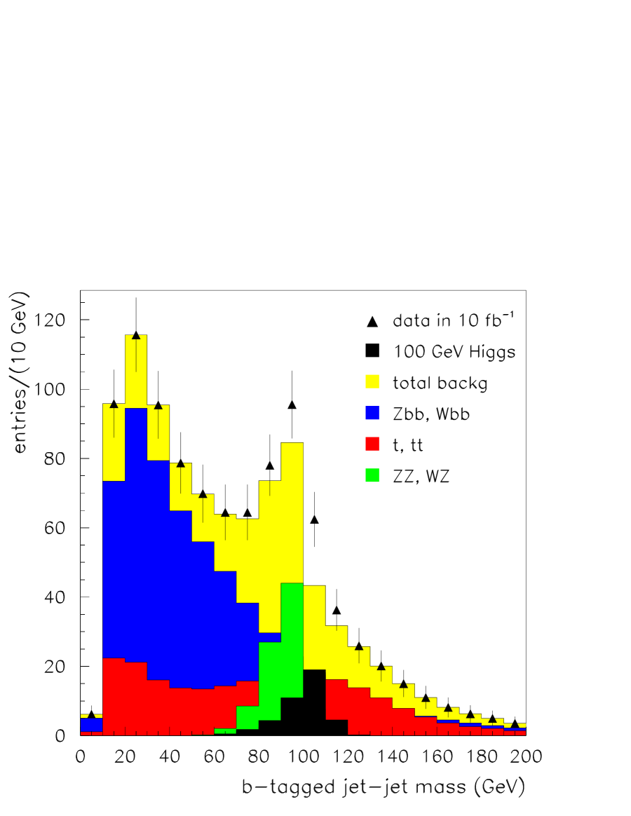
1c. , SHW Simulation and Neural Network Techniques
Event Samples \\
The events were generated using PYTHIA for Higgs masses of 90, 100, 110, 120 and 130 GeV/. The principal backgrounds to production are , , single top and . The background sample was generated using CompHEP, with fragmentation done using PYTHIA, while all other samples were generated using PYTHIA. We used SHW to simulate the detector response and, as in the study, we assumed that two jets are -tagged. The cross sections for signal and background are shown in Tables 20 and 21.
| (GeV/c2) | |
|---|---|
| 90 | 0.020 |
| 100 | 0.015 |
| 110 | 0.011 |
| 120 | 0.008 |
| 130 | 0.006 |
| backgrounds | |
| 0.35 | |
| 0.80 | |
| (pb) | |
| 1.235 | |
| 1.0 | |
| 7.5 |
| (GeV/c2) | 90 | 100 | 110 | 120 | 130 |
|---|---|---|---|---|---|
| Number of events | |||||
| 1.26 | 0.87 | 0.79 | 0.80 | 0.58 | |
| 0.61 | 0.45 | 0.61 | 1.50 | 1.42 | |
| 2.04 | 1.44 | 1.42 | 0.83 | 0.31 | |
| 0.28 | 0.05 | 0.23 | 0.44 | 0.18 | |
| total background | 2.93 | 1.94 | 2.26 | 2.77 | 1.91 |
| 0.43 | 0.45 | 0.35 | 0.29 | 0.31 | |
| 0.74 | 0.63 | 0.54 | 0.48 | 0.42 |
A network was trained for each Higgs mass and for each of the backgrounds with the following variables
-
•
of the -tagged jets
-
•
of the two leptons
-
•
– invariant mass of the -tagged jets
-
•
– invariant mass of the leptons
-
•
– sum of the transverse energy of all the jets
-
•
between the first lepton and the first -tagged jet
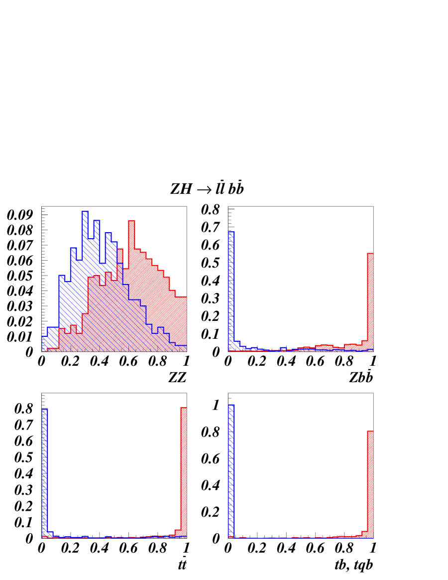
Results and Conclusions \\
Figure 55 shows the network output distributions. From these figures it is clear that discriminating between and the backgrounds is much more difficult than for and its backgrounds. Further study is needed to identify better variables if the neural network technique is to prove as powerful in this channel as in the others. We summarize the results in Table 21.
II.3.4 Channel
A. Goussiou, J. Hobbs, J. Valls, R. Vilar, D. Zeppenfeld \\
Earlier workshops tev2k ; tev33 and this study have identified the reactions and as likely modes for discovering the Higgs boson at the Tevatron. However, the great majority of events from the associated production modes and do not give final states in these channels. Roughly 70% of the final states arise from events in which the or has decayed hadronically. These modes result in a four-jet final state with two jets from the vector boson decay and two quark jets from the Higgs decay. Moreover, the same final state arises in the vector boson fusion process: (, ) when , the dominant Higgs decay mode for GeV. In the case of fusion, because there are two forward jets originating from the in the final state, one may hope to be able to suppress the Standard Model backgrounds by appropriate cuts. Three analyses of this final state are presented here. The first is an extrapolation of a published CDF Run 1 analysis and the second is a prototype analysis using a combination of SHW and data. These studies focus on the final state that arises in and production. The third is a feasibility study of the vector boson fusion process and is based on a parton-level Monte Carlo analysis.
4a. , Run 1 Extrapolation
CDF has recently published juano a search for Higgs bosons produced in association with vector bosons in pb-1 of Run 1 data. Observations are consistent with background expectation. 95% confidence level upper limits are set as a function of the Higgs mass on , with the branching ratio of the Higgs decays to . The sensitivity of the search is limited by statistics to a cross section approximately two orders of magnitude larger than the predicted cross section for standard model Higgs production. In this paper we extrapolate the results from juano to the next Tevatron Run 2 were we hope for an approximately twenty-fold increase in the total integrated luminosity as well as a significant improvement in the total acceptances.
Selection Requirements \\
The results from juano are based on a data sample recorded with a trigger which requires four or more clusters of contiguous calorimeter towers, each with transverse energy GeV, and a total transverse energy GeV. Further steps in the data reduction are: 1) four or more reconstructed jets with uncorrected GeV and . Jets are defined as localized energy depositions in the calorimeters and are reconstructed using an iterative clustering algorithm with a fixed cone of radius in space. After this initial selection the sample contains 207,604 events; 2) at least two among the four highest- jets in the event are identified (tagged) as quark candidates secvtx . There are 764 events with four or more jets and two or more -tags; 3) a cut on the transverse momentum of the system, GeV/c2 strongly discriminate against QCD direct production and flavor excitation of heavy quarks. A total of 589 events remain after this cut.
Backgrounds and efficiencies \\
The main source of background events is QCD heavy flavor production. The heavy flavor content of QCD hard processes are conventionally classified in three groups: direct production, gluon splitting, and flavor excitation. The relative contributions have been modelled with the PYTHIA Monte Carlo program PYTHIA . No attempt to estimate the normalization of this source of background directly from Monte Carlo is made due to the large number of uncertainties in the predictions.
Other backgrounds are production, + jets events with and fake double-tags. The first two are estimated from Monte Carlo and the last one from data. After trigger, kinematic and -tag requirements we expect and and + jets background events, respectively.
The combined trigger and acceptance efficiency is determined using PYTHIA followed by detector and trigger simulations. It depends on the Higgs mass and increases from for GeV/ to for GeV/. The SVX double -tagging efficiency is calculated with a combination of data and Monte Carlo samples and is with a small dependence on the Higgs mass. The total efficiency increases linearly from to for Higgs masses ranging from 70 GeV/ to 140 GeV/.
CDF Run 1 Results \\
The shape of the observed -tagged dijet invariant mass distribution is fit, using a binned maximum-likelihood method, to a combination of signal, fake double-tag events, and QCD, and + jets backgrounds. The QCD and signal normalizations are left free in the fit while the normalizations of the , + jets and fakes are constrained by Gaussian functions to their expected values and uncertainties. The fit yields pb for GeV/, statistically compatible with zero signal. For larger masses, zero signal contribution is preferred. Table 22 shows the result of the fits as a function of the Higgs mass and Figure 56 shows the -tagged dijet invariant mass distribution for the data compared to the results of the fit for GeV/.
| (GeV/) | ||||||||
|---|---|---|---|---|---|---|---|---|
| 70 | 80 | 90 | 100 | 110 | 120 | 130 | 140 | |
| Fit (pb) | ||||||||
| SM (pb) | ||||||||
| Limit (pb) | ||||||||
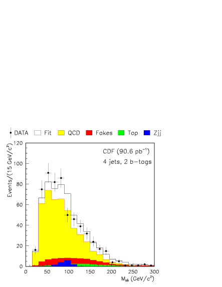
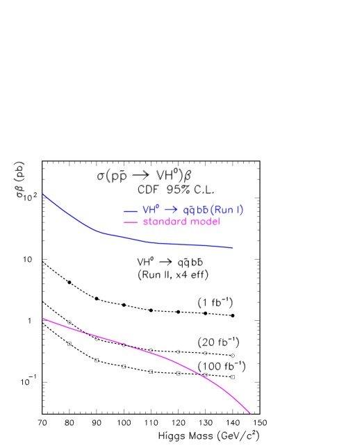

CDF Run 2 Extrapolation \\
Figure 58 shows the CDF Run 1 results for the 95% CL upper limits on as a function of the Higgs mass. In general, the obtained 95% CL statistical limits agree very well with the expected ones, except for the region of very low masses were the magnitude of the limits is strongly influenced by the fluctuation structure of the data.
A simple extrapolation to account for the expected increase in luminosity and in the total acceptances lead to improved limits by, at least, a factor .313131No account is taken here of the increase in center of mass energy from 1.8 TeV to 2.0 TeV. Here and represent the increased acceptances and luminosity factors with respect to Run 1. We consider three different luminosity scenarios for Run 2 and beyond: 1, 20 and 100 fb-1. In addition we consider the increased geometrical acceptance of the new Run 2 CDF silicon vertex detector SVX II, which will extend the -tagging capabilities up to the range . A Monte Carlo study for the process indicates a total signal improvement of in double -tag efficiencies (assuming Run 1 central -tag intrinsic efficiencies per jet). We finally consider an optimized multijet trigger for associated Higgs production in Run 2. The requirement of displaced tracks with large impact parameter at the trigger level makes it possible to relax the Run 1 multijet criteria to only 3 jets with uneven cuts and a lower threshold. A preliminary study petar shows that these cuts result on a few-fold increase in signal efficiencies without compromise the total trigger rates.
Figure 58 shows the CDF Run 1 95% CL extrapolated limits for the different luminosity scenarios combined with the roughly four times better acceptance for Run 2. Figure 58 shows the 95% CL upper limit reach as a function of the required luminosity and the Higgs mass for three different improved acceptances.
4b. , SHW Analysis
The first of these sections describes the data samples and normalizations used in the analysis. The second describes the selection criteria, and the third describes the relationship between the analysis sensitivity and hypothetical improvements in event reconstruction. The last section contains the conclusions.
Event Samples \\
For the channels considered here, the dominant background is QCD production of four jet events, two of which are -quark jets. Other backgrounds include and single- events, events, events, jet events and jet events. The relative cross sections after a basic four-jet selection are given in Table 23. One sees that the QCD multijet events completely dominate the other backgrounds. The multijet cross section in Table 23 was computed by multiplying the total four-jet cross section observed in a monitor data sample (described below) by the fraction of simulated four-jet events which have two or more -quark jets. The cross section uses the DØ published value. The remaining cross-sections are purely theoretical and were taken from either CompHep() or Pythia(all others). The QCD multijet background is roughly five orders of magnitude larger than all others. Because of this, the background calculations are made using only QCD production. All others are neglected.
| Cross Section (fb) | ||
| Sample | Total | 4-jet Accepted |
| Multijet | — | |
| 2600 | 2600 | |
| 4000 | 2700 | |
| 1400 | 900 | |
| 490 | 350 | |
| — | 2000 | |
Run 1 monitor data taken with the DØ detector were used to provide the jet rapidity and momentum distributions for the multijet background. The sample represented approximately 1 nb-1 of exposure and events were required to have passed a trigger of at least one L1 trigger tower with GeV and at least three L2 trigger jets with GeV. In addition standard quality requirements were made. The triggered sample contained approximately events. The flavor information of each jet in an event was randomly assigned according to the flavor-by-jet-rank distributions from Pythia+SHW.
Signal samples of events were generated using Pythia. The boson was forced to decay to quarks and the Higgs was required to decay to . The quark flavors in the vector boson decay were distributed according to the standard model expectation. The Pythia four-vectors were then input to SHW for detector simulation. Samples were generated for Higgs masses of 80, 90, 100, 110, 120, 130 and 140 GeV.
The final states were not directly simulated. Instead, it was assumed that the acceptance and distributions were identical to those for the modes. The mass, production cross section, and branching ratio, had of course been replaced by the corresponding quantities for the boson. Thus, we report results for inclusive production of and .
| (GeV) | Acceptance |
|---|---|
| 80 | 0.11 |
| 90 | 0.13 |
| 100 | 0.14 |
| 110 | 0.15 |
| 120 | 0.16 |
| 130 | 0.15 |
| 140 | 0.13 |
Selection Criteria \\
The analysis selection is quite simple. The requirements are:
-
•
-
•
-
•
-
•
323232For the modes, was replaced by .
-
•
.
Here is the number of cone jets in the event which satisfy and GeV. is the number of 0.5 cone jets tagged as -quark jets using the SHW -tag algorithm based on a displaced vertex or a soft lepton.333333This is a parameterization based on true jet flavor and . It includes mistag parameterizations for light quarks and -quarks. Tag jets must also satisfy and . The variables and are the difference in pseudorapidity between the two -tagged jets () and the two non-tagged jets(). The masses and are respectively the masses of the -tagged jet pair and the non -tagged jet pair in the event. For properly assigned flavors, these masses should be close to the Higgs mass and the mass . The resolution parameters and are, respectively, the RMS values of the mass distributions for the Higgs and decay products seen in simulated events.
Other simple variables (including the of the system, total energy and scalar of the four jets, rapidity boost of the and systems) have been investigated and found not to contribute significantly beyond these. The requirements arise because the signal is peaked toward narrower opening angles than the background. This arises because the and Higgs are boosted, so their decay products will on average be closer together than any given jet pair from the four jets in multijet backgrounds.
The () events should show peaks in the reconstructed dijet mass spectra near the mass for non -tagged jets and near the Higgs mass for the -tagged jets. The multijet background, on the other hand, should have no such peaks, but instead be a steeply falling distribution in both masses. This observation motivates the last two requirements which simply demand that the reconstructed masses lie near the () and Higgs masses. The distributions are shown in two-dimensional plots, for GeV, in Figure 59. In all figures, the background corresponds to a luminosity of 1 pb-1, while the signal plots correspond to 30.5 fb-1.

A number of different ways of imposing the mass condition were considered. In addition to the final choice of lower bounds on and , elliptical regions centered around the masses and diagonal lines were also considered. In the absence of backgrounds other than multijet production, the various methods gave similar results, so the simple box was chosen. If additional backgrounds, particularly top production, would be added, a requirement which also places an upper bound on the reconstructed masses might also be needed.
The effects of the selection cuts on the background and signal samples are shown in Table 25 as number of events corresponding to an integrated luminosity of 1 fb-1.
| Basic Jet Selection | , Selection | Mass Cut | |||||
|---|---|---|---|---|---|---|---|
| (GeV) | |||||||
| 80 | 58 | 860000 | 27 | 200000 | 11 | 6800 | 0.13 |
| 90 | 48 | ” | 23 | ” | 8.1 | 5400 | 0.11 |
| 100 | 38 | ” | 17 | ” | 5.6 | 3600 | 0.09 |
| 110 | 28 | ” | 12 | ” | 3.5 | 2800 | 0.07 |
| 120 | 19 | ” | 8 | ” | 2.5 | 2300 | 0.05 |
| 130 | 10 | ” | 5 | ” | 1.3 | 2000 | 0.03 |
| 140 | 4 | ” | 2 | ” | 0.45 | 1700 | 0.01 |
The data in Table 25 were used to derive luminosity requirements to achieve 95% C.L. exclusion limits, and and excesses. The significance is defined as . Here is the number of signal events for a given luminosity, and is the number of background events in the same luminosity. This measure of significance corresponds to the probability that the background fluctuates upward to at least the number of observed signal events. In all cases, one-sided, gaussian confidence intervals were used. The results are shown in Figure 60 plotted as luminosity required versus Higgs mass.

Improvements \\
There are a number of ways in which this analysis could be improved. Among them are:
-
1.
the reconstructed mass resolution is improved relative to the SHW results,
-
2.
the -quark jet identification efficiency or purity is improved and
-
3.
other analysis techniques, particularly multivariate likelihoods or neural nets, giving significantly improved background rejection or signal acceptance.
We have attempted to assess the improvements these might offer by computing the luminosity required to reach a given statistical significance for a hypothetical improvement in discrimination were made.
The most likely candidate is improved mass resolution. The current jet finding algorithm uses only calorimeter information. It has already been shown that including additional information will improve the reconstructed mass. Also, the jet corrections used in this analysis were designed only to correctly reproduce the peak positions of the mass distributions. No attempt was made to minimize the resolution. Figure 61 shows the significance versus mass resolution for GeV and 1 fb-1. This result was derived by improving the signal mass resolution by a fixed amount and making the same box selection as the standard analysis. Because is smaller, the selection requirement, , corresponds to a higher minimum mass. Thus, this procedure corresponds to a fixed acceptance (for the signal) and decreasing background. One sees that a factor of two improvement in mass resolution corresponds to a factor of four reduction in background and thus a factor of two improvement in significance.


It is also possible that as the Run 2 data are processed, we will be able to increase the -tagging efficiency or purity. Figure 61 also shows the significance as a function of tagging efficiency of the second -tagged jet. The improvement is realized by multiplying the standard SHW tag probability for the second jet by the factor shown on the abscissa with the constraint that the efficiency never exceed unity. One sees that a 50% improvement in efficiency gives only a modest gain in significance.
4c. with Forward Jet Tags
We consider the weak gauge boson fusion process, , where the quark and anti-quark both radiate vector bosons which then annihilate to produce the Higgs boson. This includes and fusion originating from all allowed combinations of initial quarks and/or antiquarks. The two scattered (anti)quarks are observed in the detector as forward jets, of to 80 GeV and provide a telltale signature for the process. Tagging these forward jets is a very powerful tool to suppress backgrounds, and has already been shown to be a highly promising tool for intermediate mass Higgs boson studies at the LHC wbfLHC .
Selection Criteria \\
Here, we concentrate on the dominant decay mode for the Higgs mass region of interest, . The Higgs boson would appear as a invariant mass peak in 4-jet events in which two of the jets are identified as quarks. Let us consider the case of GeV as an example. The signal rate is given by
| (45) |
which is reduced to about 40 fb after minimal acceptance cuts of
where and is the corresponding pseudorapidity and azimuthal angle. Here the jet separation cut is applied to all four jets, including the two -quark jets.
Backgrounds \\
An irreducible background to these signal events arises from real emission QCD corrections to production. We have calculated the SM cross section with full matrix elements, i.e. with a tree level parton Monte Carlo program. We find a cross section of 2.4 nb for this irreducible background within the minimal cuts given above and for -quark pair invariant masses above 100 GeV.
A significant reduction of the background is possible by exploiting the characteristic features of the weak boson fusion signal. The two tagging jets of the signal typically have GeV, and they are widely separated, , with the two -quark jets located between these two tagging jets, which are required to reside in opposite detector hemispheres. In addition we can increase the transverse momentum requirement for the -quark jets to 40 GeV without undue loss of signal acceptance. These additional cuts reduce the background to 30 pb for GeV while keeping a signal rate of fb.
Results and Conclusions \\
The Higgs signal would have to be seen as a invariant mass peak in this high background environment. Even assuming a invariant mass resolution of GeV, the signal to background ratio does not exceed 1/1000 within a 20 GeV invariant mass bin. Additional distributions exist which differ somewhat between the Higgs signal and the background. However, we have been unable to find cuts which significantly improve the statistical significance of the Higgs signal. The SM Higgs search via weak gauge boson fusion does not appear promising at the upgraded Tevatron.
II.3.5 Exclusive Higgs Production
M. Albrow, D. Litvintsev, P. Murat, A. Rostovtsev
There is a possibility that a light ( less than about 135 GeV) Higgs can be discovered at the Tevatron by the exclusive production process . This would lead to events with two quark jets in the central detector, and in the far forward and backward directions the scattered proton and antiproton. One could select such events by triggering on the central jets, and by measuring the trajectories of the scattered beam particles one could reconstruct very precisely the Higgs four-momentum.
The QCD process is overwhelming if one simply tries to reconstruct the di-jet invariant mass spectrum. While the mass resolution in reconstructing a jet pair at 100-130 GeV is anticipated to be about 10% as shown in the previous sections, the actual width of a Higgs in this mass region is less than 10 MeV daws , so if one can improve the mass resolution the signal to background ratio keeps improving.
In the exclusive channel there is a possibility of a factor about 50-100 improvement, limited mainly by the momentum spread of the incoming beams. The visibility of the Higgs by this technique depends on the size of the cross section for the process where the Higgs is produced (in the central region) completely exclusively, i.e. the and go down the beam pipes each having lost about in longitudinal momentum and no other particles are produced. The mechanism is as usual through intermediate loops of heavy particles (predominantly a top loop); this leaves the and in color-octet states which normally gives rise to color strings filling rapidity with hadrons. However some fraction of the time another gluon can be exchanged which neutralises (in a color sense) the and and can even leave them in their ground state. The difficulty is in calculating what this fraction is. It involves non-perturbative QCD: soft gluon calculations, soft color interactions, or Regge theory etc. In Regge theory it is the double pomeron exchange () process.
In 1990 Schäfer, Nachtmann and Schöpf scha made calculations of diffractive Higgs production at the LHC and SSC, and concluded that cross sections for the exclusive reaction could not be determined reliably. They concluded that “great effort should be invested experimentally and theoretically to better understand the properties of the pomeron and to be able to make more precise predictions.” In 1991 Bialas and Landshoff bial calculated from Regge theory that some 1% of all Higgs events may have the and in the region of very high Feynman , but did not estimate the fully exclusive process. In 1995 Cudell and Hernandez cude made a lowest order QCD calculation with the non-perturbative form factors of the proton tuned to reproduce elastic and soft diffractive cross-section measurements. They find, for the exclusive (they call this elastic) production of Higgs with = 100(130) GeV at = 1.8 TeV a cross section of about 50(30) fb, with an uncertainty about a factor of 2. The total Higgs production cross section (at 2 TeV) is about 1200(600) fb at these masses daws , so the exclusive fraction is 4% to 5%, even larger than that in the Bialas and Landshoff paper. However there are issues of “rapidity gap survival probability” and whether they are or are not implicitly included, and renormalization of the “pomeron flux”, initial and final state interactions, shadowing effects etc. All these phrases are poorly understood but are probably different ways of saying the same thing, namely that diffractive cross sections are lower than naïve Regge expectations by about an order of magnitude in hadron-hadron collisions (not in collisions). Understanding that there is a large uncertainty in this estimate, we apply a factor of 10 reduction to the estimate of ref. cude and get about 4 fb (the increase of from 1.8 to 2.0 TeV will also help).
That would mean, in Run 2 (2 fb-1) only 8 events (before applying any efficiencies). It appears that 2 fb-1 is very difficult for any Higgs searches, so we consider a Run 3 with 30 fb-1 which could give 120 events, or with 50% acceptance 60 events. This could be a discovery channel if the background is about 140 events or less. Now we come to the key of our idea.
For these exclusive events, with the Higgs produced centrally, the and each lose about in momentum, so they have . They could both be detected in Roman pot detectors and, with high resolution (10 ) tracking their momenta can be measured with very high precision (). This needs a measurement of the primary vertex (at the intersection of the two -jet directions, using SVX tracking) and good knowledge of the quadrupole, electrostatic and dipole fields from the vertex to the pots. Then the missing mass () to the measured and will have a resolution limited by the spread on the incoming beam particles’ momenta. This is about 10-4, and gives a mass resolution on the selected dijet candidates of about 200 MeV343434These numbers are still largely “back of the envelope” estimates; a proper simulation has yet to be done.. This is a factor about 50 better than the resolution on the effective mass () of the dijet and hence we get a factor 50 improvement in . Furthermore, even if the Higgs were to be discovered another way, this process has the potential of giving the best value for . We should now try to estimate the ratio to see whether there is hope that the signal could be visible.
We take CDF’s published cross section cdfb for two b-tagged jets, which starts at 150 GeV, and extrapolate down to 100(130) GeV finding 200(40) pb/GeV (in ). From our other studies, at lower mass, we expect that about of these would have a rapidity gap on each side (assuming this fraction is not -dependent). That gives 4.0(0.8) fb.GeV-1, or 0.8(0.16) fb per 200 MeV bin to be compared with a signal of around 5(3) fb in such a bin. We thus have a of order 6(20) (with the assumed reduction of the Cudell and Hernandez estimate by a factor 10). In 10 fb-1 this means 30 events on a background of 1.6 for a 130 GeV Higgs! We have not included a factor for -tagging efficiency and acceptance, but that affects both signal and background proportionately, to first order. We have also not put in the acceptance of the Roman pots for these events, which depends on Tevatron-dependent factors but should be high if the -distribution of the and is not much harder than in generic high mass diffraction.
We think it is very important to study the backgrounds as early as possible in Run 2. This means covering the region forward of = 3.5 with miniplug calorimeters (supplementing the CLC counters) and Beam Shower Counters out to the beam rapidity (). One trigger is 2 jets with nothing in both forward directions. (Looser prescaled triggers are needed to measure the non- backgrounds.) We can measure vs for generic jets and for tagged -jets out to above 100 GeV but with poor resolution and relatively wide bins. By this time we should be better able to judge how promising the Higgs search may be.
If it does look promising then, to do the Higgs search, an additional arm of Roman pot detectors must be placed on the -side after dipoles to give acceptance for down to = 0 as we have now on the -side. At present there is no warm space (spool-piece) where such pots could go. The simplest way to make such a space is by removing the Q1 quadrupoles which are redundant in Run 2 (they are being taken out at DØ) and to move the dipoles closer to the interaction point. A Beams Division study would be needed, but probably a lever arm of 1 m for pot detectors could be made, giving if positioning accuracy of 10 can be achieved (which is overkill, given the uncertainty on the incoming momenta). Moving the dipoles closer to BØ(symmetrically on the and sides) would mean moving the CDF detector by about 2 cm; we do not see that as a major problem.
This Higgs search trigger is then a high track in each forward arm, no hits in any BSC counter or either miniplug (i.e. rapidity gaps from ) and two central jets above about 20 GeV in . At a later level trigger and/or offline one selects two tagged b-jets and requires large, where is the total effective mass of the central calorimeter towers. After low missing and other clean-up cuts we would require and plot in bins dictated by the resolution. This strategy will only work for single interactions per bunch crossing, because additional interactions will spoil the gaps and pile up in . The search will be more difficult in the presence of multiple interactions but should still be possible. Precision timing on the pot tracks can (a) check that the and came from the same interaction (b) measure the position in of that interaction, and (c) correlate with the timing of the and/or jets from the time of flight barrel (in CDF). A fast trigger processor could be used to correlate and and record events when these are comparable. Off-line the cleanliness of the vertex from which the and emerged is used as a cut.
There is another process with a similar diagram to the exclusive Higgs production but with a larger cross section and this could be used to test our understanding. This is followed by . The has the same quantum numbers () as the vacuum and the Higgs. A measurement of the fraction of all (low ) which are produced in total isolation would be instructive, and could probably be made with a 2- 2-gap trigger early in Run 2. One can also study exclusive production, using the time of flight barrel in a Level 1 trigger on the or final states.
II.4 High-mass Standard Model Higgs Bosons: 130–190 GeV
Tao Han, A. Lucotte, M. Schmitt, A.S Turcot, R.-J. Zhang
As previous studies and the present studies have shown, in the Higgs mass region where the decay mode dominates the most sensitive channels are those arising from the associated production of an electroweak gauge boson and the (SM, or SM-like) Higgs boson Stange:1994ya ; GH ; steve :
| (47) |
However, as shown in the first section of this report the leading production mechanism for a SM-like Higgs boson at the Tevatron is the gluon-fusion process via heavy quark triangle loops
| (48) |
There are also contributions to production from the vector boson fusion processes353535Here and henceforth, generically denotes a boson of either on- or off-mass-shell.
| (49) |
where and are radiated from the quark partons. In Fig. 5, we present cross sections for SM Higgs boson production at the Tevatron for processes (47), (48) and (49). We see that the gluon fusion process yields the largest cross section, typically a factor of four above the associated production (47). For GeV, fusion processes become comparable to that of (47). In calculating the total cross sections, the QCD corrections have been included for all the processes 19 ; 23 ; 32 , and we have used the CTEQ4M parton distribution functions CTEQ .

Although the decay mode in Eqs. (48) and (49) would be swamped by the QCD background, the decay modes to vector boson pairs,
| (50) |
will have increasingly large branching fractions for GeV and are natural channels to consider for a heavier Higgs boson.
In Fig. 62(a), we show the cross sections for with and versus at TeV. The leptonic decay channels are also separately shown by solid and dashed curves, respectively, for
where and is a quark jet. Although the mode has a larger production rate, the mode is cleaner in terms of the SM background contamination. The corresponding modes from are smaller by about an order of magnitude. At the LHC, the channel is an important discovery mode dreiner .
It is natural to also consider the mode from the associated production in Eq. (47). It was noted Stange:1994ya that associated production with can lead to a unique like-sign lepton signature via
The production rates for these modes are denoted by solid curves in Fig. 62(b). The trilepton signal is smaller than the like-sign lepton plus jets signal by about a factor of three due to the difference of decay branching fractions to and to jets. For comparison, also shown in Fig. 62(b) are (solid) and (dashed) via . We see that the signal rates for these channels drop dramatically for a higher . Comparing the decays in Fig. 62(a) and (b), it makes the gauge boson pair modes of Eq. (50) a clear choice for Higgs boson searches beyond 130 GeV.
The purely leptonic channel in Eq. (LABEL:sigww) has been studied at SSC lnulnu and LHC energies dreiner and at a 4 TeV Tevatron GH . Despite the difficulty in reconstructing from this mode due to the two missing neutrinos, the obtained results for the signal identification over the substantial SM backgrounds were all encouraging. More recently for the 2 TeV Tevatron upgrade, there has been a parton level study parton_studies for the channels of Eq. (LABEL:sigww) and a study at the detector level for the purely leptonic channel htz of Eq. (LABEL:sigww) and like-sign lepton plus jets channel htz of Eq. (LABEL:likesign). The trilepton signature has been examined for the Tevatron and LHC Wells .
Event Samples \\
The event samples for this study were generated using the PYTHIA 6.023 event generator and SHW detector simulation. The signal cross sections have NLO QCD corrections 19 included and are based on the the CTEQ4M parton distribution functions CTEQ . For pair production of resonances, e.g. , PYTHIA incorporates the full matrix elements thereby insuring proper treatment of the final state angular correlations. Similarly for , the angular correlations between the four final state fermions have been taken into account. The full interference is simulated for production; however, the process considers only the pure contribution. For Higgs boson production in association with a gauge boson in Eq (47), the associated and decay angular distributions are treated properly. For some samples, such as where the rejection factor was high, but the cross section was also large, generator–level preselections were applied to reduce the sample passed to SHW. The production cross-sections for the principal background processes were normalized to pb, pb, pb, and pb. The measured DØ rate w3jet was used to estimate the background from with a third jet faking a electron.
II.4.1 Channel
The process can lead to the purely leptonic channel in Eq. (LABEL:sigww), where we identify the final state signal as two isolated opposite-sign charged leptons and large missing transverse energy. Such a signature has been shown to be a sensitive way to search for the Higgs in the mass range 155-180 GeV/ at the LHC dreiner .
At the Tevatron the leading SM background processes in this search are
Selection Criteria\\
We first impose basic acceptance cuts for the leptons 363636The cuts for leptons were chosen to reflect realistic trigger considerations. It is desirable to extend the acceptance in .
where is the transverse momentum and the pseudo-rapidity. The cut on the invariant mass is to remove the photon conversions and leptonic and decays. The isolation cut on removes the muon events from heavy quark () decays.373737The electron identification in the SHW simulation imposes strict isolation requirements already.


At this level, the largest background comes from the Drell-Yan process for production. However, the charged leptons in this background are very much back-to-back and this feature is also true, although to a lesser extent, for other background processes as well. On the other hand, due to the spin correlation of the Higgs boson decay products, the two charged leptons tend to move in parallel dreiner . We demonstrate this point in Figs. 64 and 64 where the distributions of the azimuthal angle in the transverse plane [] and the three-dimensional opening-angle between the two leptons [] for the signal and backgrounds are shown.383838Since we are mainly interested in the shapes of the kinematic distributions, we present them normalized to unity with respect to the total cross section with appropriate preceding cuts. This comparison motivates us to impose the cuts
| (55) |
The background can be essentially eliminated with the help of additional cuts
| (56) |
where is the relative angle between the lepton pair transverse momentum and the missing transverse momentum, which is close to 180∘ for the signal and near 0∘ for the Drell-Yan background. The two-body transverse-mass is defined for each lepton and the missing energy as
| (57) |
and the distributions are shown in Fig. 65.

We can further purify the signal by removing the high events from as well as from , as demonstrated in Fig. 67. We therefore impose
As suggested in ref. 5 , the lepton correlation angle between the momentum vector of the lepton pair and the momentum of the higher lepton () in the lepton-pair rest frame, , also has discriminating power between the signal and backgrounds. This is shown in Fig. 67. We thus select events with
| (59) |
A characteristic feature of the top-quark background is the presence of hard -jets. We thus devise the following jet-veto criteria:
Furthermore, if either of the two hard jets () is identified as a quark, the event will be also vetoed. The -tagging efficiency is taken from SHW.
The results up to this stage are summarized in Table 26 for thqqqe signal –190 GeV as well as the SM backgrounds. The acceptance cuts discussed above are fairly efficient, approximately 35% of the signal is retained while backgrounds are substantially suppressed. We see that the dominant background comes from the electroweak production, about a factor of 30 higher than the signal rate. The sub-leading backgrounds and +fake (the background where a jet mimics an electron with a probability of fake ) are also bigger than the signal. We note that although the -jet veto is effective against the background, the final results are not affected if the veto efficiency is significantly worse.


| [GeV] | 140 | 150 | 160 | 170 | 180 | 190 |
|---|---|---|---|---|---|---|
| signal [fb] | 3.9 | 4.4 | 5.2 | 4.8 | 3.6 | 2.5 |
| efficiency. [%] | 35 | 34 | 38 | 39 | 36 | 37 |
| fake | ||||||
| backgrounds [fb] | 130 | 13 | 0 | 4.4 | 2.4 | 18 |
Further Selection: Likelihood Analysis\\
One can improve the signal observability by constructing a likelihood based on some characteristic kinematic variables. We choose the variables as
-
1.
, the polar angle with respect to the beam axis of the dilepton dreiner ;
-
2.
as in Eq. (55);
-
3.
as in Eq. (55);
-
4.
as in Eq. (56);
-
5.
as in Eq. (LABEL:jetveto);
-
6.
as in Eq. (LABEL:jetveto).
We wish to evaluate the likelihood for a candidate event to be consistent with one of five event classes: a Higgs boson signal ( 190 GeV), , , or . For a single variable , the probability for an event to belong to class is given by
| (61) |
where denotes the probability density for class and variable . The likelihood of an event to belong to class is given by the normalized products of the individual for the kinematic variables:
| (62) |
The value of for a Higgs boson signal hypothesis () is shown in Fig. 68 where it can be seen that a substantial fraction of the and background can be removed for a modest loss of efficiency. The and backgrounds have similar distributions to the and have been omitted for clarity. We thus impose the requirement
| (63) |
The improved results are summarized in Table 27.
| [GeV] | 140 | 150 | 160 | 170 | 180 | 190 |
|---|---|---|---|---|---|---|
| signal [fb] | 3.1 | 3.6 | 4.5 | 4.1 | 2.9 | 2.0 |
| fake | ||||||
| backgrounds [fb] | 83 | 4.5 | 0 | 3.1 | 1.8 | 13 |

In identifying the signal events, it is crucial to reconstruct the mass peak of . Unfortunately, the mass from the decay cannot be accurately reconstructed due to the two undetectable neutrinos. However, both the transverse mass and the cluster transverse mass bho , defined as
yield a broad peak near and have a long tail below. The cluster transverse mass has a Jacobian structure with a well defined edge at . We show the nature of these two variables for the signal with GeV and the leading background in Fig. 69(a) for and (b) for after application of the likelihood cut. For a given to be studied, one can perform additional cut optimization. In Table 28, we list -dependent criteria for the signal region defined as
| (65) |
| [GeV] | 140 | 150 | 160 | 170 | 180 | 190 |
|---|---|---|---|---|---|---|
| - | 0.6 | 0.35 | 0.35 | 0.55 | 0.75 | |
| 25 | 25 | 30 | 35 | 40 | 40 | |
| min[] | 40 | 40 | 75 | 80 | 85 | 75 |
| 60 | 60 | - | - | - | - | |
| 65 | 65 | 65 | 75 | 85 | - | |
| 40 | 50 | 65 | 70 | 70 | 70 | |
| 100 | 100 | 70 | 70 | 90 | 90 | |
| - | 110 | 120 | 130 | 140 | 140 |
We illustrate the effect of the optimized cuts of Table 28 in Fig. 70, where the cluster transverse mass distribution for a GeV signal and the summed backgrounds, normalized to 30 , are shown before (a) and after the final cuts (b). A clear excess of events from the Higgs signal can be seen in Fig. 70(b). It is important to note that before application of the final cuts, the dominant backgrounds are and the +fake with other sources accounting for less than 10% of the total. Moreover, for 30 integrated luminosity, the statistical error in the background is less than 2% before application of the final cuts. We therefore argue that one should be able to normalize the SM background curve () with sufficient precision to unambiguously identify a significant excess attributable to Higgs boson signal. It should also be noted that by selectively loosening the final cuts, it is possible to maintain the same while increasing the accepted background by up to factor of 5, and the accepted signal by a factor of 2.5. This can provide a powerful cross-check of the predicted background shape and can be used to demonstrate the stability of any observed excess.
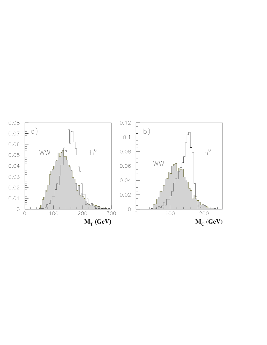
Our final results for the channel are summarized in Table 29. We have included the contributions to from the signal channels in Eqs. (47) and (49). Although they are small to begin with, they actually increase the accepted signal cross section by 12–18%. We have also included the contribution from .393939From consideration of the + background, it should be clear that improving the sensitivity by incorporating hadronic tau decays will be a difficult task. It can be seen that one may achieve a of at least 6% for 140 GeV GeV and reach 45% for GeV. The statistical significance, , for 30 fb-1 integrated luminosity, is 3 or better for GeV.
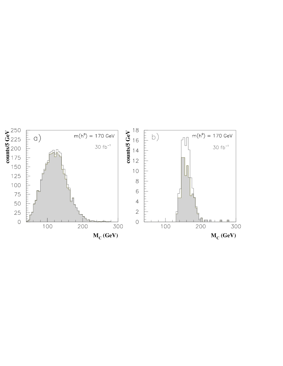
| [GeV] | 140 | 150 | 160 | 170 | 180 | 190 |
|---|---|---|---|---|---|---|
| [fb] | 2.2 | 2.4 | 1.3 | 0.93 | 0.85 | 0.73 |
| associated [fb] | 0.26 | 0.31 | 0.13 | 0.09 | 0.06 | 0.06 |
| fusion [fb] | 0.12 | 0.12 | 0.09 | 0.06 | 0.05 | 0.05 |
| signal sum [fb] | 2.6 | 2.8 | 1.5 | 1.1 | 0.96 | 0.83 |
| SM backgrounds [fb] | 39 | 27 | 4.1 | 2.3 | 3.8 | 7.0 |
| fake [fb] | 5.1 | 3.4 | 0.34 | 0.15 | 0.08 | 0.45 |
| backgrounds sum [fb] | 44 | 30 | 4.4 | 2.4 | 3.8 | 7.5 |
| 0.058 | 0.094 | 0.34 | 0.45 | 0.25 | 0.11 | |
| for 30 fb-1 | 2.1 | 2.8 | 3.9 | 3.8 | 2.7 | 1.7 |
In Fig. 71(a), we present the integrated luminosities needed to reach a 3 significance and 95% CL exclusion computed assuming Poisson probabilities as a function of .
To assess the effect of inherent systematic uncertainties, we re-evaluate the corresponding curves in Fig. 71(b) assuming a 10% systematic error for the signal and SM backgrounds.404040For the purposes of computing the effects of systematic errors on the sensitivity to a Higgs signal, we have scaled the expected background upward by a given percentage and the expected signal downward by the same percentage simultaneously. The results are somewhat degraded, but they are still encouraging.

II.4.2 Channel
For associated production, the mode can give like-sign leptons plus two-jets events Stange:1994ya ; Wells . Compared to the trilepton signature, the like-sign lepton plus jets process has a three times larger rate. Moreover, the leading SM source of like-sign and trileptons, , will generate little jet activity as both gauge bosons are required to decay leptonically to give the unique like sign signature.
The contributing channels to the final state include
The SM backgrounds are
Although the triple gauge boson production 23 in Eq. (II.4.2) constitutes an irreducible background, the , through or semileptonic decay and the background from fakes turn out to be larger. The background from background with a fake was estimated using the measured DØ rate w3jet with .


Event Selection \\
We identify the final state signal as two isolated like-sign charged leptons plus jets. A soft third lepton may be present. The basic acceptance cuts required for the leptons are
For a muon, we further demand that the scalar sum of additional track momenta within 30∘ be less than 60% of the muon momentum. We require that there are at least two jets with
| (69) |
To suppress the background, we require the leading jet to be within and to have a charged track multiplicity satisfying ; while the sub-leading jet to be within . The background typically exhibits greater jet activity; we therefore veto events having
| (70) |
and events with a fourth jet satisfying Eq. (69). The effect of the jet multiplicity and the leading jet charged track multiplicity requirements on the di-boson backgrounds can be seen in Figs. 72 and 73, respectively. To suppress backgrounds associated with heavy flavor jets, we veto the event if any of the jets have a -tag.
In Fig. 74, we present the di-jet mass distributions for the signal and backgrounds. Since the di-jets in the signal are mainly from a decay, is close to or lower than . This motivates us to further require
| (71) |
Finally, it is interesting to note that the lepton correlation angle, , has strong discriminating power to separate the signal from backgrounds as shown in Fig. 75. We then impose a final cut
| (72) |
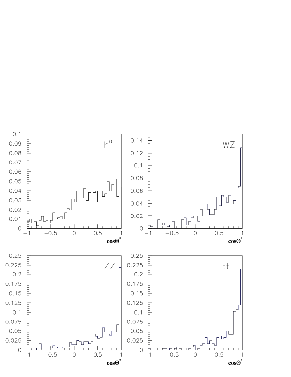
| [GeV] | 120 | 130 | 140 | 150 | 160 | 170 | 180 | 190 | 200 |
|---|---|---|---|---|---|---|---|---|---|
| signal sum [fb] | 0.093 | 0.20 | 0.34 | 0.52 | 0.45 | 0.38 | 0.29 | 0.20 | 0.16 |
| background channels | fake | Sum | |||||||
| [fb] | 0.27 | 0.06 | 0.01 | 0.15 | 0.07 | 0.02 | 0.26 | 0.83 | |
| [%] | 11 | 24 | 41 | 63 | 54 | 46 | 35 | 24 | 19 |
| [30 fb-1] | 0.56 | 1.2 | 2.0 | 3.1 | 2.7 | 2.3 | 1.7 | 1.3 | 0.96 |
With these cuts, we present the results for the signal and backgrounds in Table 30. We can see that for a given , the is larger than that for the di-lepton plus signature, reaching as high as 63%. One can consider further optimization of cuts with dependence. However, the rather small signal rate for a 30 fb-1 luminosity limits the statistical significance. Also, the systematic uncertainty in the background may be worse than the channel.
Merged Analysis \\
As described in the previous section, a final state with two same-sign leptons arises in the associated production process with decaying to (we suppress the stars for clarity of notation). One of the ’s produced in the decay will have the same sign as the primary boson, and if these two ’s both decay leptonically, a particularly clean signature results. This signature has been
developed in the search for supersymmetric particles at Run 1 in which very low background rates have been achieved. We have attempted to exploit this channel in the search for high-mass Higgs bosons.
This channel was explored in parallel by two members of the group. One of these efforts has been published htz and is described in the previous section. Later, the two analyses were merged and better performance obtained. We describe this “merged analysis” briefly in this section.
The definition of leptons and jets is retained from the analysis described above. Leptons are identified in the range and are accepted if GeV. They must be separated from all hadronic jets by , and in addition for muons, the sum of momenta of charged tracks in a cone around the muon must be less than 60% of the muon’s momentum. Jets must fall in the range and have GeV.
The selection requirements are as follows. There must be exactly two identified leptons of the same sign, and their invariant mass must be at least 2 GeV. Their isolation, computed as the sum over towers in a cone around the lepton, must be less than 3.4 GeV. Back-to-back leptons occur in background processes but rarely in the signal, so we require an acoplanarity and and acollinearity .
In contrast to the trilepton channel, we want the candidate events to show significant jet activity, expected from the hadronic decay of the third (opposite-sign) boson. There should be at least two jets but no more than six, and none of them should pass the b-tagging algorithm (impact-parameter method). To avoid -jets coming from di-boson backgrounds, we require that the two highest- jets have at least two charged tracks. Keeping in mind the mass of the , we require that these two jets have an invariant mass of no more than 200 GeV. Finally, as further evidence of high- activity, we require that the scalar sum over all calorimeter towers and muon tracks be at least 170 GeV.
The numerical values for the cuts listed above were chosen by a simple optimization program which varied all cuts simultaneously to obtain the best value for assuming in integrated luminosity of . This optimization procedure showed that some of the cuts of the two original analyses were no longer effective, and have been dropped. The signal was computed for both and production, and included decays.
Estimated backgrounds from Drell-Yan, and production are negligible. The background is serious however, and is estimated to be 0.15 fb. The background is significantly reduced with respect to the previous analysis, but still is important at 0.024 fb. Background from a or and jets is 0.15 fb based on DØ data. Contributions from triple-boson and production have been estimated and are rather small. The total background expecation is 0.48 fb.
For a SM Higgs of mass , for which the cuts above were designed, the accepted cross section is fb, giving (Table 31). For , signal events would be expected, corresponding to , for one experiment.
| (fb) | (fb) | () | ||
|---|---|---|---|---|
| 100 | 5.1 | 0.01 | 0.02 | 0.07 |
| 110 | 15.8 | 0.04 | 0.08 | 0.32 |
| 120 | 28 | 0.08 | 0.16 | 0.60 |
| 130 | 59 | 0.15 | 0.30 | 1.15 |
| 140 | 77 | 0.29 | 0.60 | 2.3 |
| 150 | 84 | 0.36 | 0.75 | 2.8 |
| 160 | 84 | 0.41 | 0.84 | 3.2 |
| 170 | 69 | 0.38 | 0.77 | 3.0 |
| 180 | 55 | 0.26 | 0.53 | 2.0 |
| 190 | 44 | 0.20 | 0.41 | 1.55 |
| 200 | 35 | 0.16 | 0.33 | 1.24 |
II.5 Higgs Bosons with Enhanced Diphoton Decay Rates
G. Landsberg, K. Matchev
The Standard Model (SM) is very economical in the sense that the Higgs doublet responsible for electroweak symmetry breaking can also be used to generate fermion masses. The Higgs boson couplings to the gauge bosons, quarks, and leptons are therefore predicted in the Standard Model, where one expects the Higgs boson to decay mostly to b-jets and tau pairs (for low Higgs masses, GeV), or to or pairs, (for higher Higgs masses, GeV). Since the Higgs boson is neutral and does not couple to photons at tree level, the branching ratio is predicted to be very small in the SM, on the order of .
In a more general framework, however, where different sectors of the theory are responsible for the physics of flavor and electroweak symmetry breaking, one may expect deviations from the SM predictions, which may lead to drastic changes in the Higgs boson discovery signatures. One such example is the so called “fermiophobic” (also known as “bosophilic” or “bosonic”) Higgs, which has suppressed couplings to all fermions, and may arise in a variety of models fermiophobe . A variation on this theme is the Higgs in certain topcolor models, which may couple to heavy quarks only topmodels . Some even more exotic possibilities have been suggested in the context of theories with large extra dimensions LED .
Finally, in the minimal supersymmetric standard model (MSSM), the width into pairs can be suppressed due to 1-loop SUSY corrections, thus enhancing the branching ratios of a light Higgs into more exotic signatures CMW1 ; Mrenna . In all these cases, the Higgs boson decays to photon pairs are mediated through a or heavy quark loop and dominate for GeV Stange:1994ya ; SMW . In the range , they compete with the mode, while for GeV, completely takes over. Current bounds from LEP LEP limits are limited by the kinematic reach of the machine. The existing Run 1 analyses at the Tevatron have utilized the diphoton plus 2 jets Lauer ; D0 ; Wilson and inclusive diphoton Wilson channels and were limited by statistics. Since they only looked for a “bosonic” Higgs, they did not consider the Higgs production mechanism through gluon fusion, which can be a major additional source of signal in certain models topmodels . Since is a very clean signature, it will allow the Tevatron to extend significantly those limits in its next run.
In this study we shall evaluate the Higgs discovery potential of the upcoming Tevatron runs for several diphoton channels. We shall concentrate on the following two questions. First, what is the absolute reach in Higgs mass as a function of the branching ratio? Second, which signature (inclusive diphotons, diphotons plus one jet, or diphotons plus two jets) provides the best reach. We believe that neither of those two questions has been adequately addressed in the literature previously.
II.5.1 Fermiophobic Higgs Bosons
Here we consider the case of a fermiophobic Higgs, i.e. models where the Higgs couplings to all fermions are suppressed. Then, the main Higgs production modes at the Tevatron are associated production, as well as fusion. All of these processes have comparable rates [see fig. 5], so it makes sense to consider an inclusive signature first Wilson .
Inclusive channel: event selection \\
We use the following cuts for our inclusive study: two photons with GeV and rapidity , motivated by the acceptance of the CDF or DØ detectors in Run 2. Triggering on such a signature is trivial; both collaborations will have diphoton triggers that are nearly fully efficient with such offline cuts.
We assume 80% diphoton identification efficiency, which we apply to both the signal and background estimates on top of the kinematic and geometrical acceptance. Again, this efficiency is motivated by the CDF/DØ EM ID efficiency in Run 1 and is not likely to change in Run 2.
Inclusive channel: background \\
The main backgrounds to the inclusive diphoton channel come from the QCD production of dijets, direct photons, and diphotons. In the former two cases a jet mimics a photon by fragmenting into a leading meson that further decays into a pair of photons, not resolved in the calorimeter.
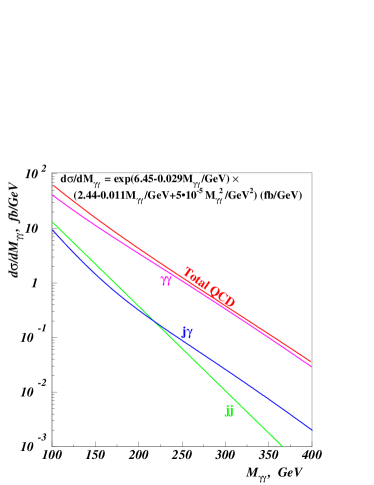
We used the PYTHIA PYTHIA event generator and the experimentally measured probability of a jet to fake a photon Lauer to calculate all three components of the QCD background. The faking probability depends significantly on the particular photon ID cuts, especially on the photon isolation requirement (see, e.g., ref. Lauer ; diboson ; monopole ). For this study we used an -dependent jet-faking-photon probability of
which is obtained by taking the -averaged faking probabilities used in the DØ Run 1 searches Lauer . The fractional error on is about 25% and is dominated by the uncertainty on the direct photon fraction in the sample used for its determination. (For high photon , however, the error is dominated by the available statistics.) This probability is expected to remain approximately the same in Run 2 for both the CDF and DØ detectors. We used 80% ID efficiency for the pair of photons, and required the photons to be isolated from possible extra jets in the event. We accounted for NLO corrections via a constant -factor of 1.34.
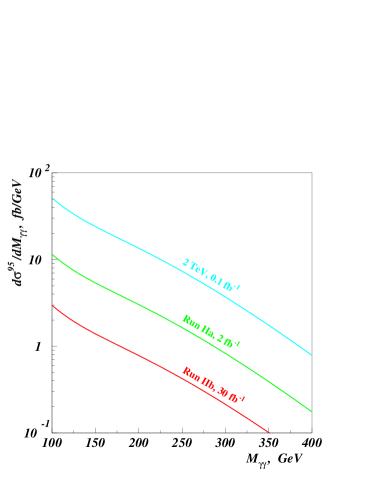
Adding all background contributions, for the total background in the inclusive diphoton channel we obtain the following parametrization:
where , , , and . In the region GeV it is dominated by direct diphoton production and hence is irreducible. The expected statistical plus systematic error on this background determination is at the level of 25%, based on the jet-faking photon probability uncertainty. For larger invariant masses, however, the accuracy is dominated by the uncertainties in the direct diphoton production cross section, which will be difficult to measure independently in Run 2, so one will still have to rely on the NLO predictions. On the other hand, for narrow resonance searches one could do self-calibration of the background by calculating the expected background under the signal peak via interpolation of the measured diphoton mass spectrum between the regions just below and just above the assumed resonance mass. Therefore, in our case the background error will be purely dominated by the background statistics. A combination of the interpolation technique and the shape information from the theoretical NLO calculations of the direct diphoton cross section is expected to result in significantly smaller background error in Run 2.
The total background, as well as the individual contributions from , and production, are shown in Fig. 76. Additional SM background sources to the inclusive diphoton channel include Drell-Yan production with both electrons misidentified as photons, production, etc. and are all negligible compared to the QCD background. The absolute normalization of the background obtained by the above method agrees well with the actual background measured by CDF and DØ in the diphoton mode Wilson ; monopole .
In Fig. 77 we show the 95% CL upper limit on the differential cross section after cuts as a function of the diphoton invariant mass , given the above background prediction (here is the product of the acceptance and all efficiencies). This limit represents sensitivity to a narrow signal when doing a counting experiment in 1 GeV diphoton mass bins. This plot can be used to obtain the sensitivity to any resonance decaying into two photons as follows. One first fixes the width of the mass window around the signal peak which is used in the analysis. Then one takes the average value of the 95% C.L. limit in across the mass window from Fig. 77 and multiplies it by , where is the width of the mass window414141The square root enters the calculation since the significance is proportional to the background to the power., to obtain the corresponding 95% CL upper limit on the signal cross-section after cuts. Similar scaling could be used if one is interested in the 3 or 5 reach.
Inclusive channel: optimum mass window \\
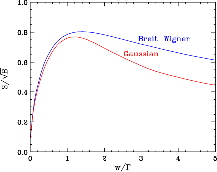
When searching for narrow resonances in the presence of large backgrounds (), the best sensitivity toward signal () is achieved by performing an unbinned maximum likelihood fit to the sum of the expected signal and background shapes. However, simple counting experiments give similar sensitivity if the size of the signal “window” is optimized. For narrow resonances the observed width424242Notice that the width is defined so that the cross-section at away from the peak is a factor of 2 smaller than the peak value (FWHM). For a Gaussian resonance the width is related to the variance by . is dominated by the instrumental effects, and is often Gaussian. The background in a narrow window centered on the assumed position of the peak in the signal invariant mass distribution could be treated as linear. Therefore, the Gaussian significance of the signal, , as a function of the window width, , is given by:
| (73) |
where erf is the error function
The function (73) is shown in Fig. 78, and has a maximum at , which corresponds to cut around the resonance maximum.
For resonances significantly wider than the experimental resolution, the shape is given by the Breit-Wigner function, and in this case the significance is:
| (74) |
This function, also shown in Fig. 78, peaks at a similar value of (). We see that for both Gaussian and Breit-Wigner resonances, the significance does not appreciably change when using a cuts. For our analysis we shall use two representative choices: and for the mass window, which we shall always center on the actual Higgs mass.
Clearly, one can do even better in principle, by suitably resizing and repositioning the mass window around the bump in the combined distribution. Because of the steeply falling parton luminosities, the signal mass peak is skewed and its maximum will appear somewhat below the actual physical mass. In our analysis we choose not to take advantage of these slight improvements, thus accounting for unknown systematics.
Inclusive channel: results \\
In Tables 32 and 33 we show the inclusive background rates in fb for different Higgs masses, for and mass window cuts, respectively.
| Significance | ||||||||||
|---|---|---|---|---|---|---|---|---|---|---|
| bknd | jet | jets | ||||||||
| (GeV) | (fb) | |||||||||
| 100. | 271.7 | 16.5 | 31.3 | 34.2 | 36.3 | 35.4 | 31.9 | 36.4 | 35.1 | 31.1 |
| 120. | 166.6 | 13.0 | 24.4 | 26.7 | 28.5 | 28.5 | 24.7 | 29.5 | 29.2 | 26.7 |
| 140. | 103.0 | 10.7 | 20.1 | 22.4 | 23.9 | 23.9 | 20.6 | 24.0 | 23.7 | 21.0 |
| 160. | 64.3 | 8.9 | 17.0 | 19.1 | 20.1 | 20.4 | 17.2 | 20.2 | 20.8 | 19.2 |
| 180. | 40.5 | 7.3 | 13.5 | 15.0 | 16.2 | 16.5 | 13.6 | 16.3 | 16.7 | 16.2 |
| 200. | 26.1 | 5.8 | 10.6 | 11.9 | 12.5 | 12.7 | 10.4 | 12.3 | 12.7 | 12.0 |
| 250. | 9.4 | 3.7 | 6.7 | 7.5 | 7.9 | 8.2 | 6.6 | 7.9 | 8.7 | 8.4 |
| 300. | 4.8 | 2.2 | 3.8 | 4.3 | 4.7 | 4.7 | 3.6 | 4.2 | 4.9 | 4.7 |
| 350. | 2.3 | 1.5 | 2.8 | 3.1 | 3.3 | 3.3 | 2.4 | 2.8 | 3.0 | 3.4 |
| 400. | 1.2 | 1.0 | 1.8 | 2.0 | 2.0 | 2.1 | 1.7 | 1.7 | 2.1 | 2.4 |
| Significance | ||||||||||
|---|---|---|---|---|---|---|---|---|---|---|
| bknd | jet | jets | ||||||||
| (GeV) | (fb) | |||||||||
| 100. | 453.4 | 14.4 | 27.0 | 29.8 | 31.7 | 30.6 | 27.7 | 31.9 | 30.5 | 26.4 |
| 120. | 278.1 | 11.3 | 21.3 | 23.5 | 25.1 | 24.9 | 21.9 | 25.5 | 25.1 | 22.5 |
| 140. | 171.9 | 9.3 | 17.5 | 19.5 | 21.0 | 21.0 | 17.7 | 20.7 | 21.0 | 18.5 |
| 160. | 107.3 | 8.0 | 15.1 | 16.7 | 18.0 | 18.2 | 15.4 | 17.8 | 18.2 | 17.3 |
| 180. | 67.6 | 6.6 | 12.2 | 13.7 | 14.6 | 14.9 | 12.4 | 14.3 | 15.2 | 14.2 |
| 200. | 43.6 | 5.4 | 10.1 | 11.4 | 12.1 | 12.1 | 9.9 | 11.9 | 12.3 | 11.1 |
| 250. | 15.7 | 3.6 | 6.5 | 7.3 | 7.7 | 7.8 | 6.4 | 7.6 | 8.5 | 8.0 |
| 300. | 8.1 | 2.1 | 3.8 | 4.2 | 4.6 | 4.5 | 3.6 | 4.3 | 4.5 | 4.5 |
| 350. | 3.9 | 1.6 | 2.7 | 3.0 | 3.4 | 3.4 | 2.6 | 3.1 | 3.5 | 3.1 |
| 400. | 2.1 | 1.1 | 1.9 | 2.2 | 2.3 | 2.4 | 1.6 | 2.1 | 2.6 | 2.4 |
Here we have added the intrinsic width and the experimental resolution in quadrature: . The width varies between 3.5 GeV for GeV and 29.0 GeV for GeV. The two tables also show the significance (for 1 fb-1 of data, and assuming ) in the inclusive diphoton channel when only associated production and fusion are included in the signal sample. We see that (as can also be anticipated from Fig. 78) a cut around the Higgs mass typically gives a better statistical significance, especially for lighter (and therefore more narrow) Higgs bosons.
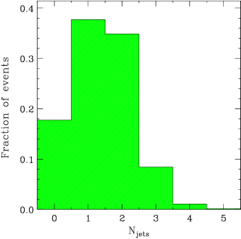

Exclusive channels: event selection \\
The next question is whether the sensitivity can be further improved by requiring additional objects in the event. The point is that a significant fraction of the signal events from both associated production and fusion will have additional hard objects, most often QCD jets. In Fig. 79 we show the “jet” multiplicity in associated production, where for detector simulation we have used the SHW package with a few modifications as in SHWmod . Here we treat “jets” in a broader context, including electrons and tau jets as well.
Previous studies Wilson ; D0 have required two or more additional QCD jets. Here we shall also consider the signature with at least one additional “jet”, where a “jet” is an object with . The advantages of not requiring a second “jet” are twofold. First, in this way we can also pick up signal from fusion, whose cross-section does not fall off as steeply with , and in fact for GeV is larger than the cross-section for associated production434343In the case of a topcolor Higgs (see the next section) we would also pick up events with initial state gluon radiation, comprising about 30% of the gluon fusion signal, which is the dominant production process for any Higgs mass.. Events from fusion typically contain two very hard forward jets, one of which may easily pass the jet selection cuts. This is illustrated in Fig. 80, where we show the pseudorapidity distribution of the two spectator jets in (a) associated production and (b) fusion. Second, by requiring only one additional jet, we win in signal acceptance. In order to compensate for the corresponding background increase, we shall consider several thresholds for the additional jet, and choose the one giving the largest significance.
For the exclusive channels we need to rescale the background from Fig. 76 as follows. From Monte Carlo we obtain reduction factors of , , , and for the jet channel, with , 25, 30 and 35 GeV, respectively. For the jets channel the corresponding background reduction is , , , and , depending on the jet cuts. These scaling factors agree well with those from the CDF and DØ data from Run 1.
Notice that we choose not to impose an invariant dijet mass () cut for the jets channel. We do not expect that it would lead to a gain in significance for several reasons. First, given the relatively high jet cuts needed for the background suppression, there will be hardly any background events left with dijet invariant masses below the (very wide) mass window. Second, the signal events from fusion, which typically comprise about of our signal, will have a dijet invariant mass distribution very similar to that of the background. Finally, not imposing the cut allows for a higher signal acceptance because of the inevitable combinatorial ambiguity for the events with jets.
The significances for the two exclusive channels, with the four different jet cuts, are also shown in Tables 32 and 33. We see that the exclusive jets channel with GeV typically gives the largest significance, but our new exclusive jet channel is following very close behind.
Exclusive channels: results \\
We are now ready to present our results for the Run 2 Tevatron reach for a bosonic Higgs. In Fig. 81 we show the 95% CL upper limit on the branching ratio , with 0.1 (cyan), 2.0 (green) and 30 (red), as a function of . For each mass point, we compare the significance for both the inclusive as well as the exclusive channels with all the different cuts, and for the limit we choose the channel with the set of cuts providing the best reach.
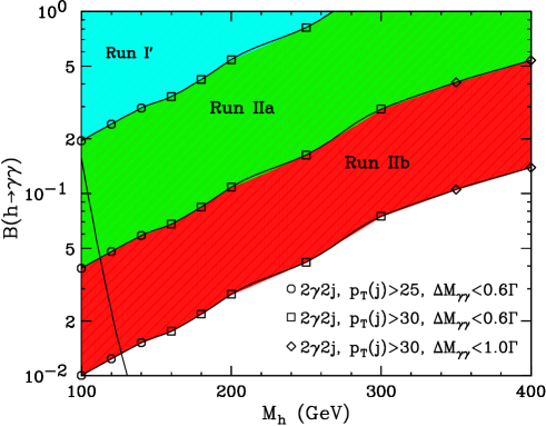
It turns out that for this case the optimal selections are
-
o:
, with GeV and ,
-
:
, with GeV and , and
-
:
, with GeV and .
In the figure we also show the HDECAY hdecay prediction for in case of a “bosonic” Higgs. The reach shown for 0.1 is intended as a comparison to Run 1, in fact for the 0.1 curve we scaled down both the signal and background cross-sections to their values at 1.8 TeV center-of-mass energy, keeping the efficiencies the same. In other words, the region marked as Run 1′ would have been the hypothetical reach in Run 1, if the improved Run 2 detectors were available at that time. As seen from Fig. 81, the reach for a “bosonic” Higgs (at 95% CL) in Run 2a and Run 2b is GeV and GeV, correspondingly. This is a significant improvement over the ultimate reach from LEP LEP limits of GeV.
II.5.2 Topcolor Higgs Bosons
Here we consider the case of a “topcolor” bosonic Higgs, where the Higgs also couples to the top and other heavy quarks topmodels . We therefore include events from gluon fusion into our signal sample. We used next-to-leading order cross-sections for gluon fusion hxsec .
In Tables 34 and 35 we show the significance (for 1 fb-1 of data, and again assuming ) in the inclusive and the two exclusive channels, for the topcolor Higgs case. Since gluon fusion, which rarely has additional hard jets, is the dominant production process, the inclusive channel typically provides the best reach. However, the channel is again very competitive, since the additional hard jet requirement manages to suppress the background at a reasonable signal cost. We see that our new channel clearly gives a better reach than the channel Lauer ; D0 ; Wilson . For Higgs masses above GeV, it sometimes becomes marginally better even than the inclusive diphoton channel. The specific jet cut and mass window size seem to be less of an issue – from Tables 34 and 35 we see that , GeV and GeV work almost equally well, and for GeV both values of are acceptable.
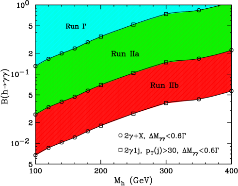
| Significance | ||||||||||
|---|---|---|---|---|---|---|---|---|---|---|
| bknd | jet | jets | ||||||||
| (GeV) | (fb) | |||||||||
| 100. | 271.7 | 54.3 | 43.4 | 44.6 | 45.1 | 42.5 | 33.6 | 37.8 | 36.4 | 32.1 |
| 120. | 166.6 | 42.5 | 35.3 | 36.9 | 37.3 | 35.3 | 26.5 | 30.8 | 30.2 | 27.5 |
| 140. | 103.0 | 35.5 | 30.4 | 32.1 | 33.0 | 31.6 | 22.3 | 25.6 | 25.1 | 22.0 |
| 160. | 64.3 | 30.1 | 27.3 | 28.8 | 29.2 | 28.3 | 19.5 | 22.4 | 22.4 | 20.3 |
| 180. | 40.5 | 24.5 | 22.4 | 23.8 | 24.5 | 23.8 | 15.7 | 18.2 | 18.3 | 17.6 |
| 200. | 26.1 | 19.9 | 18.6 | 19.9 | 20.3 | 20.0 | 12.7 | 14.4 | 14.3 | 13.3 |
| 250. | 9.4 | 12.9 | 12.5 | 13.3 | 13.6 | 13.4 | 8.4 | 9.7 | 10.2 | 9.8 |
| 300. | 4.8 | 9.1 | 8.7 | 9.3 | 9.6 | 9.4 | 4.9 | 5.6 | 5.9 | 5.9 |
| 350. | 2.3 | 8.4 | 7.9 | 8.4 | 8.4 | 7.9 | 4.0 | 4.1 | 4.5 | 4.5 |
| 400. | 1.2 | 6.4 | 6.1 | 6.1 | 6.3 | 6.2 | 3.0 | 3.0 | 3.5 | 3.1 |
| Significance | ||||||||||
|---|---|---|---|---|---|---|---|---|---|---|
| bknd | jet | jets | ||||||||
| (GeV) | (fb) | |||||||||
| 100. | 453.4 | 47.7 | 37.6 | 38.9 | 39.5 | 36.9 | 29.0 | 33.0 | 31.6 | 27.1 |
| 120. | 278.1 | 37.7 | 31.2 | 32.6 | 33.1 | 31.2 | 23.5 | 26.6 | 25.9 | 23.1 |
| 140. | 171.9 | 31.4 | 26.7 | 28.2 | 29.0 | 27.9 | 19.2 | 22.1 | 22.0 | 19.4 |
| 160. | 107.3 | 26.6 | 24.3 | 25.3 | 26.0 | 25.2 | 17.4 | 19.7 | 19.5 | 18.3 |
| 180. | 67.6 | 22.3 | 20.5 | 21.7 | 22.1 | 21.6 | 14.2 | 16.2 | 16.8 | 15.4 |
| 200. | 43.6 | 18.8 | 17.7 | 19.1 | 19.4 | 18.9 | 12.0 | 13.7 | 13.8 | 12.5 |
| 250. | 15.7 | 12.8 | 12.1 | 13.2 | 13.4 | 13.1 | 8.2 | 9.3 | 10.0 | 9.6 |
| 300. | 8.1 | 9.0 | 8.5 | 9.1 | 9.2 | 9.0 | 5.0 | 5.6 | 5.6 | 5.7 |
| 350. | 3.9 | 8.3 | 7.6 | 8.1 | 8.1 | 7.9 | 4.0 | 4.7 | 4.6 | 4.4 |
| 400. | 2.1 | 6.3 | 6.1 | 6.3 | 6.3 | 6.1 | 2.9 | 3.4 | 3.7 | 3.6 |
In Fig. 82 we show the Run 2 reach for the branching ratio as a function of the Higgs mass, for the case of a “topcolor” Higgs boson. This time the channels with the best signal-to-noise ratio are: o: inclusive , and : , with GeV; both with .
Summary \\
We have studied the Tevatron reach for Higgs bosons decaying into photon pairs (for an alternative study with similar results, see MW ). For purely “bosonic” Higgses, which only couple to gauge bosons, the channel offers the best reach, but the channel is almost as good. For topcolor Higgs bosons, which can also be produced via gluon fusion, the inclusive channel is the best, but the channel is again very competitive. We see that in both cases the channel is a no-lose option!
II.6 Enhanced MSSM Neutral Higgs Boson Production at Large
M. Roco, A. Belyaev, J. Valls
This section of the report presents a study to evaluate the sensitivity reach of the Fermilab Tevatron for the neutral Higgs bosons of the Minimal Supersymmetric Standard Model produced in association with bottom quarks, with (). Due to the strongly enhanced couplings at large , this channel becomes potentially important since it can be the dominant production and decay modes of the neutral Higgs bosons over a large region of the parameter space.
The events of interest would have four jets in the final state, two of which come from a Higgs resonance. In this Workshop two analyses have been performed, emphasizing the different strengths of the two detectors and different aspects of the signature. Each analysis is described in the next two sections, and a comparison made at the end.
DØ Analysis \\
This analysis is based on Monte Carlo simulations which have been tuned to the existing DØ detectors in a well-studied environment. It is assumed that it will be possible to maintain the excellent performance of the DØ calorimeter during Run 2. The -tagging algorithm described in Section II.A.3 is used in this analysis.
Monte Carlo Simulation \\
All signal and background event samples used in this analysis were generated using the CompHEP package comphep . CompHEP performs calculations of complete tree-level matrix elements for all parton processes with up to five partons in the final state. It has been interfaced with Pythia V6.023 spythia to simulate the parton fragmentation and hadronization. Events were generated at a center-of-mass energy, TeV. The generation of the signal and background Monte Carlo samples and the relevant tree-level cross section calculations are described in more detail in ref. sasha .
Detector Simulation \\
The signal detection efficiencies and accepted background cross sections are estimated using a fast detector simulation package, MCFAST mcfast . MCFAST performs parameterized tracking where for each generated track, a covariance matrix is assembled, which represents all the material and detector planes traversed by the ideal track. A reconstructed track is produced by smearing the generated track parameters according to this covariance matrix.
Particle momenta are smeared as prescribed in SHW using 20 and 80 for the electromagnetic and hadronic energy resolutions, respectively. The reconstruction of calorimeter clusters (jets) is based on the cone algorithm with a fixed cone radius .
The beam vertex is centered at the origin with a smearing of 30 m in both and and 25 in . In this study only one interaction per beam crossing is considered.
Signal Event Samples \\
This analysis uses only the leading order cross sections for the signal production process. Next-to-leading order corrections DSSW can be significant at the Tevatron, ranging from for 40 GeV to for 1000 GeV. It was also shown in DSSW that the largest uncertainty in the production cross section comes from varying the factorization scale, . In this analysis, the scale is chosen. Signal cross sections are determined using a running -quark mass, with varying from 3.4 to 3.1 GeV in the Higgs mass range between 90 to 300 GeV. Table 36 lists the the production cross sections for for the pseudoscalar Higgs boson , in femtobarns for 1. The cross sections after applying parton-level kinematic cuts on and are also given in Table 36. The decay branching ratios for are obtained from HDECAY hdecay . It is assumed that the SUSY particles are heavy enough such that the decays of Higgs bosons into them are kinematically forbidden.
| (fb) | (fb) | ||
|---|---|---|---|
| (GeV/c2) | (GeV/c2) | no cuts | 15 GeV/c |
| and 0.5 | |||
| 90 | 3.40 | 13.820 | 0.7492 |
| 100 | 3.38 | 8.628 | 0.5224 |
| 110 | 3.36 | 5.831 | 0.3730 |
| 120 | 3.34 | 3.730 | 0.2556 |
| 130 | 3.32 | 2.563 | 0.1924 |
| 140 | 3.30 | 1.733 | 0.1366 |
| 200 | 3.22 | 0.255 | 0.0271 |
| 250 | 3.18 | 0.064 | 0.0076 |
| 300 | 3.14 | 0.018 | 0.0024 |
Backgrounds \\
The dominant backgrounds come from QCD multi -jet production. These include the irreducible backgrounds from and , as well as the reducible backgrounds from and events with the mistagging of a light quark (), charm or gluon jet as a -jet. Table 37 lists the leading order cross sections in picobarns for the background processes considered in this study. The value of is set to 15 GeV/c for the and processes. This value is raised to 25 GeV/c for to obtain statistically significant samples after applying the selection criteria described below. From Table 37, a serious background arises from QCD production which is several orders of magnitude larger than the signal cross section. Reducing this overwhelming background requires a -tagging algorithm with a very high purity. Other background processes, such as production and , are less important and have negligible contributions after the analysis cuts are applied.
| Process | |
|---|---|
| and 0.5 | |
| 3.3 * 0.15 BR() | |
| 3.1 * 0.68 BR() | |
| 2.4 | |
| 1610.8 |
Event Selection \\
The final state is characterized by two clear signatures, the four-jet topology and a high -quark content. These properties are the main handles for suppressing the enormous QCD multi-jet backgrounds. Events are passed through a filtering algorithm intended to select hadronic events compatible with the four-jet topology and to use the -tagging information to reduce the dominant QCD backgrounds. The efficient identification of jets arising from quark production plays an important role in the search for the Higgs bosons since for sufficiently large values the neutral Higgs bosons decay predominantly to with a branching ratio of about 90.
The significance of the signal can be further improved by reconstructing the Higgs mass. The di-jet mass is reconstructed only from the -tagged jets resulting in a number of possible pair-wise combinations, . Using these combinations, it may be possible to define a smooth combinatoric background distribution with an overall normalization which can be determined from the data. Otherwise, it becomes difficult to determine the significance of a mass peak if, for instance, one takes only the combination closest to the assumed Higgs mass.

 \\
\\

The first level of event selection is performed to filter and select events which satisfy Run 1 multi-jet trigger requirements of at least four reconstructed jets in the event with 15 GeV and . The spectra of the leading jets are determined by the Higgs mass. This is illustrated in Figure 83 where the distributions of the four leading jets are shown for two signal samples, with = 100 GeV/c2 and = 200 GeV/c2. For comparison, the bottom plot shows the jet spectra for the irreducible QCD background (this plot was generated using a sample with a cut of 15 GeV/c). The following selection criteria on the of the leading jets are chosen to optimize the significance, , where and are the number of signal and background events, respectively, remaining after cuts:
-
leading jet
-
second leading jet max
-
third and fourth leading jets 30 GeV
Figure 84 shows the optimal values for the leading jet cut for four different values of the Higgs mass.
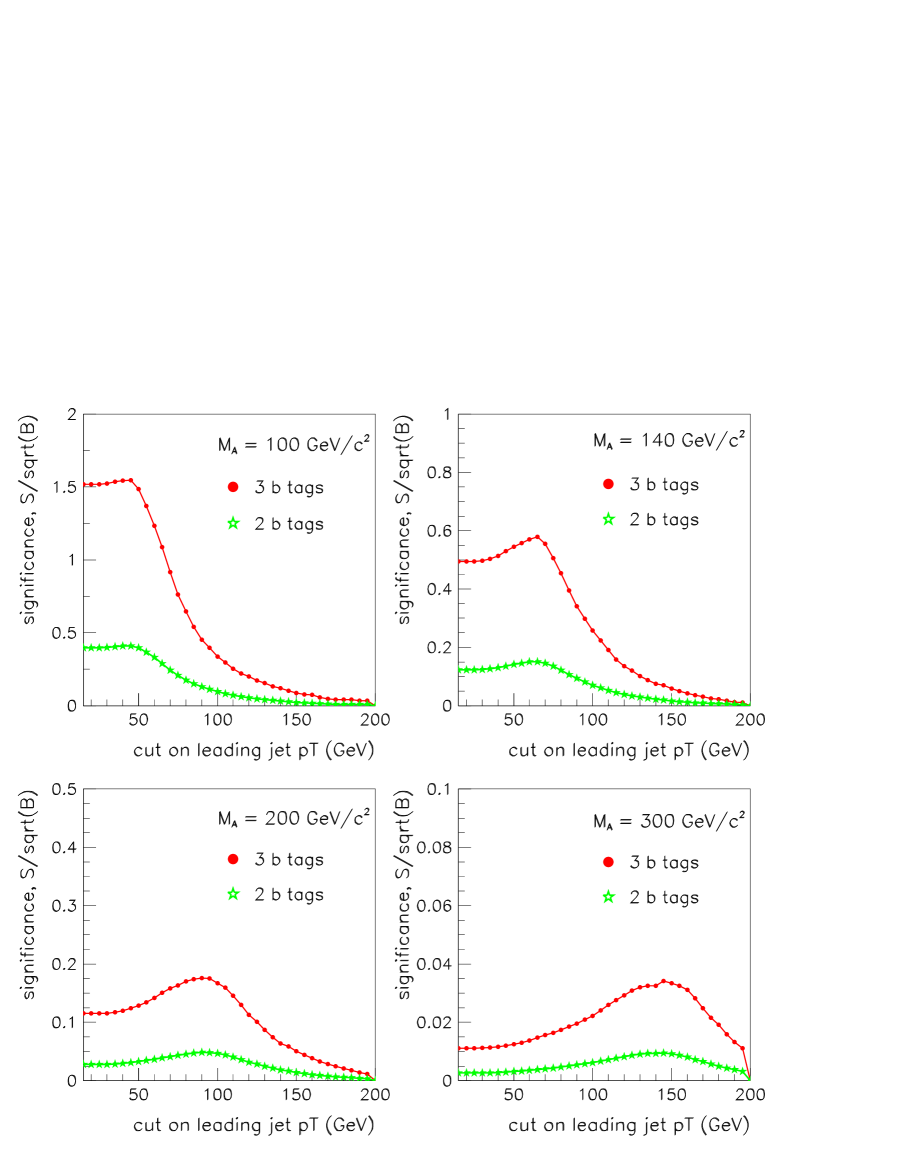
The requirement on the third and fourth jets is determined by the value of the cut used to generate the Monte Carlo samples. The selection criteria require that at least three of the four leading jets are -tagged. Table 38 lists the signal acceptances for the single channel , where is calculated after requiring the multi-jet triggers. The are calculated after the trigger and jet cuts are applied, and requiring at least two, three or four -tags, respectively. The total efficiency refers to the remaining events after the nominal selection requiring at least three -tags. Table 39 lists the number of expected events passing the selection criteria for the pseudoscalar Higgs signal and the various background processes, for an integrated luminosity of fb-1. The sensitivities and are given for = 40.
| (GeV/c2) | () | () | () | () | () | () |
|---|---|---|---|---|---|---|
| 90 | 3.46 0.03 | 27.46 0.22 | 68.87 0.24 | 34.36 0.41 | 5.23 0.30 | 0.33 0.01 |
| 100 | 3.97 0.03 | 30.95 0.22 | 69.38 0.26 | 36.79 0.37 | 5.62 0.28 | 0.45 0.01 |
| 110 | 4.39 0.04 | 33.32 0.21 | 70.75 0.28 | 36.90 0.35 | 6.64 0.28 | 0.54 0.01 |
| 120 | 4.81 0.04 | 35.63 0.20 | 70.17 0.30 | 36.27 0.34 | 6.50 0.27 | 0.62 0.01 |
| 130 | 5.39 0.04 | 36.43 0.20 | 71.32 0.30 | 38.14 0.33 | 6.46 0.26 | 0.75 0.02 |
| 140 | 5.78 0.05 | 37.69 0.20 | 70.81 0.31 | 38.37 0.32 | 6.60 0.26 | 0.84 0.02 |
| 200 | 8.20 0.06 | 38.72 0.19 | 72.08 0.33 | 38.26 0.30 | 6.33 0.24 | 1.21 0.02 |
| 250 | 9.47 0.07 | 38.63 0.19 | 70.87 0.33 | 37.12 0.30 | 7.23 0.25 | 1.36 0.03 |
| 300 | 10.78 0.08 | 38.15 0.19 | 71.07 0.33 | 36.25 0.30 | 6.80 0.24 | 1.49 0.03 |
| Higgs Mass | 90 | 100 | 110 | 120 | 130 | 140 | 200 | 250 | 300 |
|---|---|---|---|---|---|---|---|---|---|
| (GeV/c2) | |||||||||
| 0.090 | 0.078 | 0.063 | 0.046 | 0.038 | 0.029 | 0.006 | 0.002 | 0.000 | |
| 0.83 | 0.81 | 0.77 | 0.68 | 0.53 | 0.34 | 0.003 | 0.001 | 0.001 | |
| 144 | 125 | 101 | 74 | 61 | 46 | 10 | 3 | 1 | |
| 0.91 | 0.91 | 0.91 | 0.91 | 0.90 | 0.90 | 0.90 | 0.90 | 0.89 | |
| 2384 | 2225 | 2149 | 1999 | 1873 | 1571 | 598 | 297 | 127 | |
| 373 | 349 | 312 | 280 | 243 | 207 | 72 | 32 | 14 | |
| 111 | 108 | 102 | 95 | 85 | 76 | 36 | 19 | 10 | |
| 27 | 27 | 26 | 24 | 22 | 21 | 13 | 8 | 5 | |
| Total Background | 2895 | 2709 | 2589 | 2398 | 2223 | 1875 | 719 | 356 | 156 |
| 0.050 | 0.046 | 0.039 | 0.031 | 0.028 | 0.025 | 0.014 | 0.008 | 0.005 | |
| 2.68 | 2.39 | 1.98 | 1.52 | 1.30 | 1.07 | 0.37 | 0.15 | 0.07 |
Tagging Issues \\
For comparison, the total number of events passing the selection criteria which require two instead of three -tags are 235 and 1.46 events for the signal (assuming ) and background, respectively, with 100 GeV/c2. Due to the very small signal-to-background ratio, using only two -tags is not reliable for this production mode. Requiring that all four leading jets to be tagged would have the advantage of eliminating the and backgrounds. However, the signal event rate becomes substantially degraded. This study indicates that the signal to background ratio , at 100 GeV/c2, increases from 0.046 to 0.113 while the statistical significance of the signal decreases from 2.39 to 1.47. This decrease is due to the fourth jet being typically considerably softer than the third jet in the signal events as shown in Figure 83.
Let us examine the case where the -tag requirement is relaxed such that the three -tags do not necessarily have to be from the four leading jets. In this case, for 100 GeV/c2 and three -tags, there are 168 signal events with an estimated background of 2898 giving a significance of . Requiring four -tags improves the sensitivities with 0.244 and 3.52.
To simplify the algorithm for reconstructing the Higgs mass for candidate events, the selection requires that only -tags from the four leading jets are considered. This analysis is performed by requiring only three -tagged jets on account of the substantial loss of statistical significance in requiring four -tags. Tagging efficiencies are based only on displaced tracks coming from secondary vertices, not including soft lepton tags. Soft lepton tagging of jets will increase the overall -tagging efficiency, however, this has not been considered in this study. The analysis performs full vertex reconstruction and -tagging on an event-by-event basis, i.e., tagging efficiencies are not based on any rate parameterization.
Higgs Mass Reconstruction \\
One does not know a priori which -jets resulted from the Higgs decay. For each combination of tagged jets , the di-jet invariant mass is reconstructed. There are either four or six possible di-jet combinations for each event. To reduce the combinatoric background from incorrect di-jet combinations, further cuts are applied. The jets are required to be well separated azimuthally: , where the values of range from (70o,290o) for 90 GeV to (120o,240o) for 300 GeV. Alternatively, one can also use the variable to impose jet isolation.
Finally, a cut on the invariant mass of the di-jet candidate is necessary to further suppress the remaining QCD backgrounds. The di-jet mass resolution of the system coming from the Higgs decay is . For the signal event sample, all di-jet combinations which are reconstructed within of the Higgs mass constitute the signal S. Similarly, for the background samples, all di-jet combinations which are reconstructed within of the assumed Higgs mass constitute the background B.
Combining , , \\
At sufficiently large values, one of the CP-even Higgs bosons and the pseudoscalar have similar couplings and are degenerate in mass as illustrated in the following plots. The program hmsusytev.f hehprog is used to derive the couplings and masses. In Figure 85 the ratios of the CP-even Higgs couplings to as a function of pseudoscalar mass are shown for the case of maximal and minimal mixing. Figure 86 shows the mass differences () and () versus the pseudoscalar mass for different values in the maximal (top plots) or minimal (bottom plots) mixing scenarios.
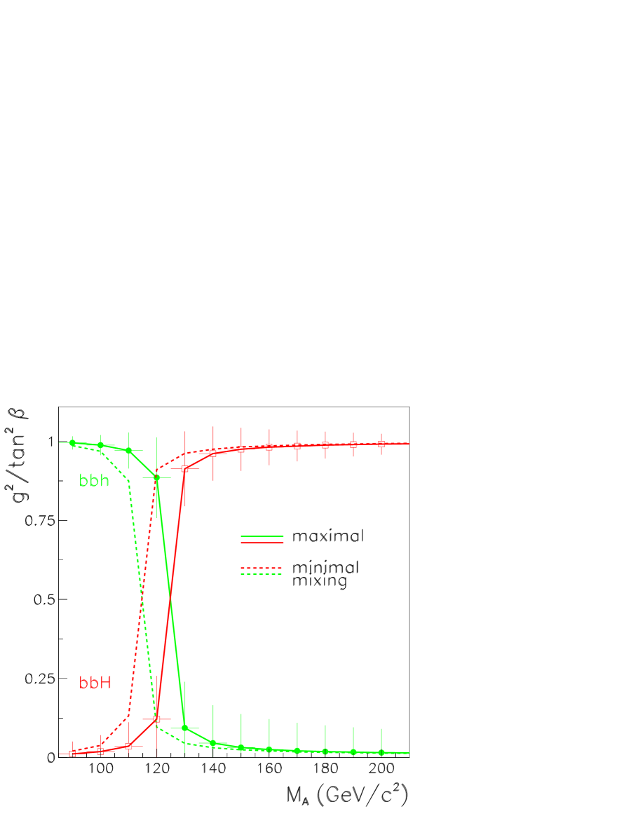
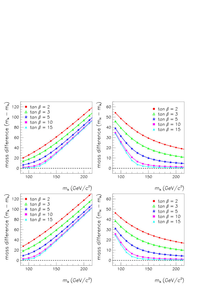
The couplings and the degree of mass degeneracy determine the additional contribution from the CP-even Higgs bosons which should be added to the pseudoscalar Higgs signal. In the case of maximal mixing, the light Higgs coupling for GeV is roughly equal to . This is also the case for the heavy Higgs coupling for GeV. However, it is not correct to simply double the signal from production since the additional contribution from may not be within the 2.5 mass window. Figure 86 shows that the mass differences between the scalar Higgs bosons and pseudoscalar are large for small values. Doubling the production rate would lead to an overestimate of the signal at low . This analysis assumes that the shapes of the di-jet mass distributions for the CP-even and the pseudoscalar Higgs bosons are identical, except for a shift in the mass peaks due to the mass differences () and (). It is also assumed that the relative normalization of the mass distributions is given by the ratio . The additional contribution from the Higgs scalars is determined by the fraction of the mass distributions within the 2.5 mass window around the assumed pseudoscalar mass .
Results \\
The signal and background estimates described above are used to estimate the discovery potential and exclusion reach for the Higgs bosons of the MSSM. For a given luminosity and an assumed Higgs mass, one can determine the minimum value of leading to a 5 discovery () or exclusion at 95 CL (1.96). The results are shown in Figure 87. The sensitivity reach in the and parameter space is shown for different values of the delivered luminosity per experiment. These results were obtained assuming maximal mixing, where SUSY parameters are chosen to give the largest predicted value for the Higgs mass. For comparison the LEP excluded region ( GeV/c2) is also shown.
In the intermediate Higgs mass range, these results indicate that the Run 2 sensitivity reach, assuming , is about 160 GeV/c2 at 95 CL exclusion with a delivered luminosity of 2 fb-1, extending up to 190 GeV/c2 with 5 fb-1. The 5 discovery reach is up to 115 GeV/c2 at 2 fb-1 and 150 GeV/c2 at 5 fb-1. For larger Higgs masses, the sensitivity reach degrades significantly due to the decreasing production rates.
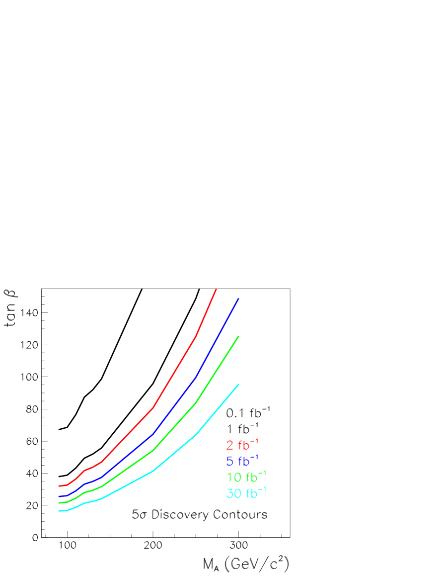
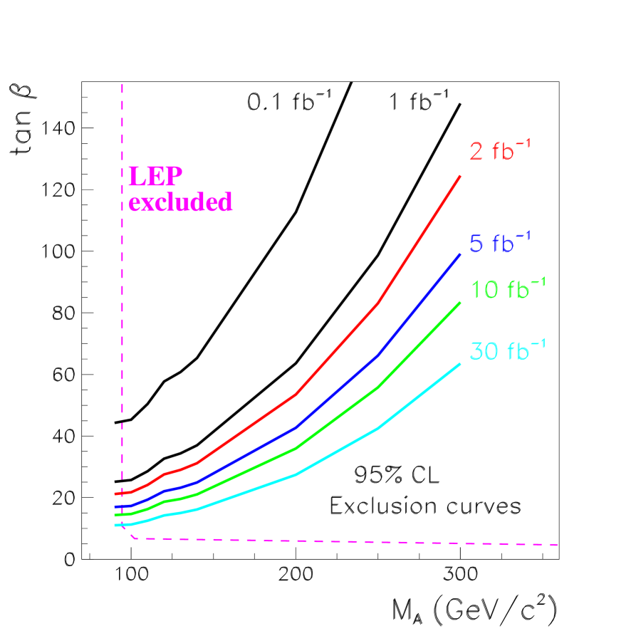
The estimates for signal efficiencies and backgrounds are affected by various systematic effects, such as the imperfect modeling of the physics processes and the detector response. Uncertainties arising from the inaccurate description and reconstruction of the energy flow, as well as the initial and final state radiation have not been studied. The main source of uncertainty in this analysis arises from the evaluation of the QCD multi -jet backgrounds. Additional factors which strongly influence the background estimates presented here include the predictions for QCD multi-jet production, the parton density distributions, the choice of scale for and higher-order corrections. Another critical issue which have not been evaluated is the effect of high luminosity conditions where the impact of overlapping interactions may become important.
Summary \\
This report has presented a strategy to search for the neutral Higgs bosons of the Minimal Supersymmetric Standard Model, where the Higgs bosons are produced in association with bottom quarks. Prospects for 5 discovery and 95 CL exclusion in the process , with , have been presented. Results indicate that the Tevatron Run 2 sensitivity reach, assuming , is about 160 GeV/c2 at 95 CL exclusion with a delivered luminosity of 2 fb-1, extending up to 190 GeV/c2 with 5 fb-1. The 5 discovery reach is up to 115 GeV/c2 at 2 fb-1 and 150 GeV/c2 at 5 fb-1. These results demonstrate that the Tevatron can significantly constrain a large fraction of the MSSM parameter space by studying the production of the neutral Higgs bosons produced in conjunction with quark pairs.
CDF analysis\\
The CDF-based analysis represents an extrapolation of the technique used in the analysis of CDF Run 1 data to the new detector geometry and improved -tagging efficiency anticipated in Run 2. The estimates of background are made from Run 1 data, with appropriate scaling for improved acceptance and efficiency444444No correction for the increased center-of-mass energy is made to either the Higgs signal or the background. This should be conservative in that, all else being equal, the sensitivity should increase with center-of-mass energy.
Figure 88 show the expected rates for production at large as a function of the Higgs mass. In this regime () is either or for masses below the light Higgs upper bound, or either the or for masses above the light Higgs upper limit. All rates are shown for the case of vanishing mixing parameters or non-mixing case defined by with the Higgs mass parameter and and the soft SUSY Yukawa breaking parameters. In all cases, a top quark mass of GeV/c2 and a SUSY mass scale of TeV are assumed. To calculate the Yukawa coupling we use a running bottom quark mass evaluated at the Higgs mass scale ( GeV/c2). All cross sections are evaluated at leading order (LO) with the CTEQ3 parton distributions functions and the renormalization scale equal to the Higgs mass.
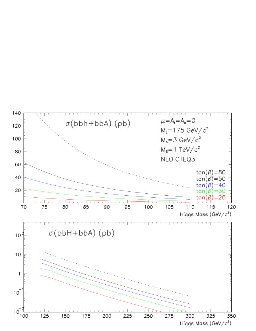
Signal Monte Carlo Simulation \\
For signal modelling we used a modified version of the parton level Monte Carlo program PAPAGENO papageno together with the Lund PYTHIA V5.6 string fragmentation and hadronization program PYTHIA . Fixed weight events with are generated at leading order (LO) and fragmented inside PYTHIA. The mass of the Higgs has been set to values between =70 GeV/c2 to 300 GeV/c2. In order to setup parton showers and fragmentation using PYTHIA, the color-flow information for colored particles is treated properly. Both initial and final state showering are allowed at energy scales corresponding to the Higgs mass. After fragmentation, events are then passed through the CDF Run 1 simulation and reconstruction code.
Event Selection \\
The CDF Run 1 multijet trigger requirements are used as the first step in the data selection. This sample is defined by events that satisfy:
-
a)
total trigger cluster GeV, and
-
b)
4 trigger clusters with GeV
where a level 2 (L2) trigger cluster is defined by a nearest-neighbor reconstruction algorithm, seeded by a tower of GeV and including only towers of GeV. The event selection follows by requiring events with at least four offline reconstructed jets with GeV and . Jets are defined as localized energy depositions in the calorimeters and are reconstructed using an iterative clustering algorithm with a fixed cone of radius in space. Jet energies are then corrected for energy losses in uninstrumented detector regions, energy falling outside the clustering cone, contributions from underlying event and multiple interactions, and calorimeter nonlinearities.
| (GeV/c2) | ||||||||||||
|---|---|---|---|---|---|---|---|---|---|---|---|---|
| 70 | 80 | 90 | 100 | 110 | 120 | 130 | 140 | 150 | 200 | 250 | 300 | |
| (GeV) | ||||||||||||
| (GeV) | ||||||||||||
| (GeV) | ||||||||||||
The typical topology of the signal events consist of two primary quarks and a Higgs , which is radiated from one of the primary quarks. There is, thus, a very high energetic primary quark with momentum of the order of the mass of the Higgs boson, , balanced by the Higgs and the other primary quark, which is generally much softer. The Higgs decays into a pair with typical transverse momentum of the order of . The four highest- (uncorrected) jets in the event are then ordered in :
| (75) |
and a mass dependent requirement made for , , and . The thresholds for these cuts are shown in Table 40 as a function of the Higgs mass. They have been optimized by maximizing the significance of the signal.
Figure 89 shows the the , distributions for two different signal Higgs masses ( GeV/c2) compared with the QCD background shapes.

We then require that at least three among the four highest- jets in the event are identified (tagged) as quark candidates. We use the CDF secondary vertex algorithm secvtx with the intrinsic Run 1 efficiencies and mistag rates per jet inside the SVX fiducial region. The results are then applied to jets at generator level within the increased geometrical acceptance of the Run 2 CDF silicon vertex detector (SVX-II). The SVX-II extends the -tagging capabilities up to the range . The -tagging algorithm begins by searching for secondary vertices that contain three or more displaced tracks. If none are found, the algorithm searches for two-track vertices using more stringent track criteria. A jet is tagged if the secondary vertex transverse displacement from the primary one exceeds three times its uncertainty.
Table 41 shows the trigger efficiency (), efficiencies (), double -tag () and triple -tag () efficiencies, and total efficiencies () as a function of the Higgs mass. The double and triple -tag efficiencies are calculated after the trigger and cuts are applied. The total efficiency applies to the triple -tag selection. All errors shown are statistical only.
Figure 90 shows the reconstructed dijet invariant mass distribution for different signal masses. The invariant mass of the dijet system is defined as . The distributions contain a Gaussian core with a resolution of –% depending slightly on the Higgs mass. To maximize the signal dijet mass resolutions we use the reconstructed invariant mass of the highest- jets in the event for masses GeV/c2. For masses GeV/c2 we use the invariant mass of the second and third highest- jets in the event. In all cases, the two highest- jets in the event are always required to be tagged. The tails of the distributions are dominated by the cases where the jet assignment in the mass reconstruction is incorrect. In most of these cases, one of the jets assigned to the Higgs is a primary quark jet.

| (GeV/c2) | (%) | (%) | (%) | (%) | (%) |
|---|---|---|---|---|---|
| 70 | |||||
| 80 | |||||
| 90 | |||||
| 100 | |||||
| 110 | |||||
| 120 | |||||
| 130 | |||||
| 140 | |||||
| 150 | |||||
| 200 | |||||
| 250 | |||||
| 300 |
Backgrounds \\
Backgrounds for the process include all sources of standard model heavy flavor multijet events. These include QCD heavy flavor production, fake multitags, (, ), + jets (), and .
QCD \\
The dominant source of background is QCD heavy flavor production. This is also the most difficult to estimate due to uncertainties in the predicted total rates as well as heavy flavor jet rates. Rather than attempting to estimate the QCD background rates directly from Monte Carlo, instead we follow the approach used in juano in the search for standard model Higgs bosons via (). In juano , the CDF Run 1 multijet data sample was used to calculate first the double tagged dijet invariant mass distribution. The shape of this distribution is then fit, using a binned maximum-likelihood method, to a combination of signal, QCD heavy flavors, fake double tags and other standard model backgrounds. The QCD heavy flavor and signal normalizations are left free in the fit while the rest of backgrounds are constrained by Gaussian functions to their expected values and uncertainties. Fake double tags are estimated from data while the other physics backgrounds are calculated from Monte Carlo. The double -tag data selection as well as details of the fit can be found in juano .
The fit yields zero signal contribution for the process for all signal masses. The results of the fit are shown in Table 42. The QCD heavy flavor background expectations are now corrected for the () and triple -tag acceptances corresponding to the present analysis. QCD heavy flavor acceptances have been calculated with the PYTHIA Monte Carlo program with its QCD leading order hard scattering processes and parton shower modelling. A sufficiently large number of events were generated with a hard scattering GeV/c in order to obtain unbiased and statistically significant samples. Below this bin no events satisfy the trigger requirements. Fake triple tag rates are calculated directly from Run 1 data using fake tagging rate parametrizations. Table 43 shows the expected QCD heavy flavor and QCD fake rates as obtained from data for the selection described in this analysis and after extrapolated to a Run 2 total integrated luminosity of 1 fb-1.
As a comparison, Table 44 shows the expected initial rates for the individual and total QCD processes leading to heavy flavors in the final state as obtained from PYTHIA. Also shown are the QCD acceptances and expected events for 1 fb-1 integrated luminosity for the present analysis. The heavy flavor content in QCD events are conventionally classified in three groups: direct production (), flavor excitation (), and gluon splitting () in initial or final state shower evolution. The relative contributions to the total cross sections are very uncertain and depend on the center of mass energy, the modelling of initial and final state radiation, shower evolution and fragmentation.
| data | QCD heavy flavors | Fakes | + jets | ||
|---|---|---|---|---|---|
| events |
| QCD heavy flavors | QCD fakes | Total QCD | |
|---|---|---|---|
| (GeV/c2) | (events per fb-1) | ||
| 70 | |||
| 80 | |||
| 90 | |||
| 100 | |||
| 110 | |||
| 120 | |||
| 130 | |||
| 140 | |||
| 150 | |||
| 200 | |||
| 250 | |||
| 300 | |||
+ jets \\
Background events have been simulated using the HERWIG herwig v5.6 Monte Carlo generator with GeV/c2. The trigger efficiency has been estimated to be from simulation. The measured CDF cross section of xs is used to estimate the expected number of events. Total initial rates and acceptances are summarized in Table 45. The errors shown include both statistical and systematic uncertainties. Systematics are dominated by the effect of the absolute energy scale, modelling of initial state radiation in HERWIG, and -tag efficiencies.
| (pb) | N | ||||||
|---|---|---|---|---|---|---|---|
| GeV/c) | (%) | (%) | (%) | (%) | (%) | (events/fb-1) | |
| Total | |||||||
| (pb) | (%) | (%) | (%) | (%) | (%) | |
|---|---|---|---|---|---|---|
| () | ||||||
| +jets | ||||||
| () | ||||||
| () | ||||||
| () |
+ jets \\
The jets background has been studied with a combination of data and Monte Carlo. The CDF measured cross sections for + jets, vj1 and + jets, vj2 are used to normalize Monte Carlo production cross sections for jet events. Generic + jets and + jets samples generated with the HERWIG Monte Carlo program vj3 and processed through the CDF simulation package were used to estimate the expected contributions after our selection cuts. The predominant source of heavy flavor production in jets events is jets () as well as some contribution of initial and final state gluon splitting and higher order diagrams leading to and events.
Table 45 shows the initial cross sections and estimated acceptances for all the + jets backgrounds leading to heavy flavor final states. The errors shown include both statistical and systematic uncertainties. The systematic uncertainties are dominated by the normalization of the measured cross sections to the predicted Monte Carlo cross sections.
Figure 91 shows the individual and total efficiencies as a function of the Higgs mass for the signal and the different standard model background contributions.

| (GeV/c2) | (events per fb-1) | |||||
|---|---|---|---|---|---|---|
| 70 | ||||||
| 80 | ||||||
| 90 | ||||||
| 100 | ||||||
| 110 | ||||||
| 120 | ||||||
| 130 | ||||||
| 140 | ||||||
| 150 | ||||||
| 200 | ||||||
| 250 | ||||||
| 300 | ||||||
| (GeV/c2) | () | () | ||
|---|---|---|---|---|
| 70 | ||||
| 80 | ||||
| 90 | ||||
| 100 | ||||
| 110 | ||||
| 120 | ||||
| 130 | ||||
| 140 | ||||
| 150 | ||||
| 200 | ||||
| 250 | ||||
| 300 | ||||
Results \\
Table 46 shows the expected number of events from each individual background contribution as well as the total backgrounds for 1 fb-1. Table 47 shows the expected number of signal events for (Standard Model case) and for as well as the signal significances as a function of the Higgs mass for 1 fb-1.
The reconstructed dijet invariant mass for the highest- jets in the event (with both jets required to be -tagged) and with present CDF Run 1 dijet resolutions is shown in Figure 92 for both signal and background. All rates are normalized to 1 fb-1.
Figure 93 shows the 95% CL exclusion limits, discovery thresholds and discovery thresholds in the – plane of the MSSM for four different total integrated luminosity scenarios, pb-1, 2 fb-1, 10 fb-1 and 30 fb-1. Figure 94 shows the required luminosity for 95% CL exclusion limits, and discovery thresholds as a function of the Higgs mass for the MSSM scenario with = 10 and 40.
In a theory with a non-minimal Higgs sector (beyond the SM), the coupling differs from the corresponding coupling of the Standard Model Higgs boson. As a result, the production cross-section for , is given by
| (76) |
where [] is the [] coupling. It is convenient to define a ratio of the Higgs production amplitude in the general model divided by the corresponding SM amplitude. In terms of the cross-sections, , where
| (77) |
Figure 95 shows the enhancement factor as a function of the Higgs mass, the integrated total luminosity, and for 95% CL, and discovery thresholds. The factor contains the entire model dependence of the cross-section and allows one to present the results in a model-independent way.


Comparison of analyses \\
Starting from quite different input assumptions and methods, the two analyses discussed above arrive at quite similar estimates for the exclusion and discovery reach for the MSSM scalar and pseudoscalar Higgses at large .
The first main difference is that the analyses use different Monte Carlo generators; the DØ analysis uses COMPHEP, whereas the CDF analysis uses a generator developed during the Workshop from a modified version of PAPAGENO with PYTHIA fragmentation. The cross sections and kinematic distributions from the two generators agree reasonably well.
The two kinematic selections proceed along similar lines, both demanding four jets. The DØ analysis demands a minimum jet transverse momentum of 30 GeV and leading and next-to-leading jet ’s which increase with Higgs mass. The CDF analysis demands GeV and four jets with a minimum of 15 GeV transverse energy.454545This is motivated by the Run 1 trigger requirements, which may loosen for Run 2 if the experiment uses the SVT to tag secondary vertices in three-jet events.
Though there are potentially four taggable jets in the signal, both analyses require three tags for optimal sensitivity. The DØ analysis assumes a tagging efficiency based on the Monte Carlo study of Section II.A.3, which has a maximum efficiency of 55%. The CDF analysis uses, conservatively, the Run 1 tagging efficiencies per taggable jet, but the much larger Run 2 detector geometry to determine taggability. This is perhaps the largest source of difference between the two analyses, since the cube of the tagging efficiency determines the signal rate.
By far the largest background comes from QCD production, and the CDF simulations of its total rate did not agree with the observed rate in analyses of Run 1 data. The only weapons against it are the requirement of the third tag and reconstructing the Higgs mass. The DØ analysis relies on Monte Carlo simulations of the background, and the CDF analysis uses Monte Carlo scaled by a factor determined with Run 1 data, and taking into account the increased center of mass energy in Run 2. Given the different signal selections, it is difficult to say how well the two methods agree.
The two analyses also take different approaches to Higgs mass reconstruction. The DØ analysis uses all possible combinations in an event, and a 15% resolution (for the correct combination) based on the MC studies. The CDF analysis uses jets 1 and 2 at high Higgs masses, and jets 2 and 3 at lower Higgs masses. The assumed resolution is that of Run 1, typically 15% for the correct combination for a 150 GeV/ Higgs mass.
All these differences nevertheless lead to quite similar estimates for exclusion and discovery. Since the reach in goes as the square of the cross section limit, the 30-40% lower reach of the DØ analysis implies that the two analyses differ by perhaps 15-20% in the end. Such differences are easily understood in the context of the foregoing paragraphs.
Both analyses assume rather conservative tagging efficiency and mass resolution; these are quite likely to be better in the actual run. Furthermore, the role of an improved trigger should be studied further; the fact that in many events one of the jets is very far forward could perhaps mean that it is optimal to require only three jets in the central region.
In any case, this search represents the main mode for discovering or ruling out the MSSM Higgs at large , and demonstrates one of the unique advantages of hadron colliders.
II.7 Charged Higgs Bosons
Dhiman Chakraborty
In this section we consider the prospects for discovering or excluding charged Higgs bosons produced in decays of top quarks at the Tevatron in Run 2. If a charged Higgs boson exists, then it can be directly produced in collisions. However, as shown in Section I.C.5.b, the cross section for inclusive charged Higgs production is probably too small to be seen at the upgraded Tevatron if . However, if is kinematically allowed then it can compete with , which is by far the dominant decay mode of top quark in the Standard Model (SM).
As previously noted, if , and if is either very small or very large, then a significant fraction of those events could contain charged Higgs bosons. We focus on a search for based on the Type II two-Higgs doublet model (2HDM) where one doublet couples exclusively to the down-type fermions, and the second doublet couples exclusively to up-type fermions hhg .464646The MSSM Higgs sector is a Type II 2HDM. However, the analysis of this section is more general, since the results depend only on the charged Higgs boson mass and the parameter which parameterizes the coupling of to fermion pairs [see eq. I.3.1]. No MSSM relations among Higgs sector parameters are imposed.
Recent results from searches for charged Higgs bosons can be found in refs. TEV ; LEP ; CLEO ; ALEPH2 . This study is an extension of a search performed by DØ based on 109 pb-1 from Run 1 TEV .
Parameter space
In the region , the total inclusive cross-section for the production of either and/or is given by:
| (78) |
in the approximation that . The parameters and uniquely fix the top quark branching ratios, given the top quark mass. In this analysis, we use the theoretical prediction that include NLO QCD corrections ttbarxsec : pb at TeV. However, only tree-level formulae for the top-quark branching ratios have been employed. Fig. 96 shows the region of the [,] plane examined in this study. The minimum for is chosen at 50 GeV, somewhat below the most recent lower limits from LEP.
This search is restricted to GeV, somewhat less than (assuming GeV); otherwise, the width of the charged Higgs becomes too large ( GeV) near the upper boundary on , and leading-order calculations become unreliable. For the same reason, is required to be GeV. Since GeV, irrespective of [,], this amounts to requiring , and thereby excludes from our analysis the dark-shaded regions at the two bottom corners of Fig. 96. The cross-hatched regions correspond to . Also shown in Fig. 96 are the decay modes of that dominate in different parts of the parameter space. Analogous charge-conjugate results hold for .

Methodology of a disappearance search
A direct search (or “appearance search”) for charged Higgs bosons covering the entire parameter space is made difficult by the variety of final state signatures. The region dominated by suffers from enormous QCD backgrounds. While it is possible to look directly for , and for , both DØ and CDF have found that an indirect “disappearance” search was a competitive option in Run 1 TEV .
With increasing statistics and enhanced detector performance, direct searches will gain strength faster than a disappearance search, but the latter, the only one considered in this study, is expected to dominate until the integrated luminosity exceeds fb-1.
In a disappearance search, one employs selection criteria optimized to detect the SM decay of . Such criteria are expected to have relatively low efficiency for decays involving . The top quark pair-production cross section is not expected to be significantly affected by the presence of a charged Higgs. Consequently, if data agree well with SM-based predictions for , regions of parameter space where is large can be excluded because in those regions one would expect fewer events than seen in data. We have considered final states containing one or two charged leptons ( or ), as was done in Run 1 analyses, although it is possible that all-hadronic final states also will be utilized in future.
The published values of the production cross section () and the mass of the top quark () from direct observation at DØ d0cs ; d0mt and CDF cdfcs ; cdfmt are based on the assumption of BR() = 1. The topic of present interest is based on a violation of this assumption, so those measurements are not relevant in our analysis. Hence, in the process of setting limits in the [,] plane, the values of and serve as input parameters.
Signal, background, and their modeling
Our search for , are based on selection criteria optimized for events which are detailed in refs. d0cs ; cdfcs . jets and jets are the main sources of physics background, while measurement fluctuations resulting in false identification of electrons, muons, and neutrinos () in QCD multijet events contribute to instrumental background.
All events are simulated using ISAJET ISAJET and a GEANT-based simulation of the Run 1 DØ detector. The efficiencies are verified using PYTHIA PYTHIA , and improvements for Run 2 are estimated from studies conducted in the course of the technical design report for DØ upgrade, as well as SHW. jets and jets events are modeled using the VECBOS tree-level parton generator interfaced with ISAJET for fragmentation and hadronization. The instrumental background is estimated using Run 1 data d0cs ; d0mt ; cdfcs ; cdfmt , on which additional suppression factors expected from detector improvements are applied.
Event selection
The final states of decaying according to the SM are characterized by the decays of the two bosons in the event. We focus on events where at least one decays into an , or a , and the associated neutrino. If the other also decays into or , then the event is classified as a “dilepton” event. If it decays into , we call it a “single lepton” event. Dilepton events are characterized by two high- isolated leptons, large , and two or more jets, both originated by quarks. Single lepton events are characterized by one high- isolated lepton, large , and three or more (nominally, four) jets, two of which are originated by quarks. Tagging of the -quark jets, either by a decay vertex separated from the primary interaction vertex, or by an associated non-isolated lepton from semileptonic decay of offers strong suppression of backgrounds in single-lepton channels. Backgrounds in dilepton channels are so small that the -tag requirement is not necessary.
| single-lepton | dilepton | |
| 20 GeV | 20 GeV | |
| 2.0 | 2.0 | |
| 20 GeV | 20 GeV | |
| leptons () | ||
| 20 GeV | 20 GeV | |
| 2.0 | 2.0 | |
| jets () | ||
| -tags | 1 or 2 | |
| Aplanarity | 0.04 | – |
| 110 GeV | 110 GeV |
The selection criteria for dilepton and single-lepton channels are summarized in Table 48. These are similar to those used to measure in Run 1 d0cs ; cdfcs . In addition to these cuts, any event with an identified lepton (hadronic decays only) with GeV and is rejected. The dilepton and single-lepton selection criteria are combined in a logical OR, so an event passing both sets of cuts is counted only once, not twice.
Efficiencies
For each top quark, there are four possible decay modes whose branching fractions depend on and : (1) ; (2) , ; (3) ; and (4) . If the decay mode of () is denoted by (), then the total acceptance for any set of selection criteria is given by
| (79) |
where is the efficiency for channel , and is the branching fraction. All depend strongly on both and ; depends on neither, and all other depend on , but not on .
The efficiencies for various channels, for = 110 GeV, are given in Table 49 in the form of a symmetric matrix. The 10 independent elements of the matrix are plotted as functions of in Figs. 97 and 98. Uncertainties in jet energy scale, particle identification, and signal modeling are the main components of systematic uncertainties. The total systematic uncertainty is estimated to be 10% of the efficiency. Statistical uncertainties are negligible.
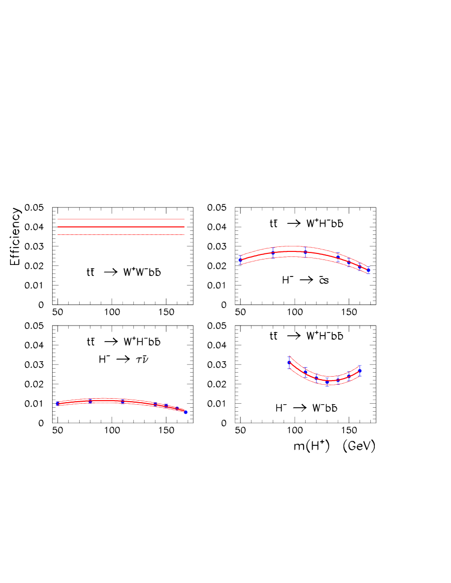
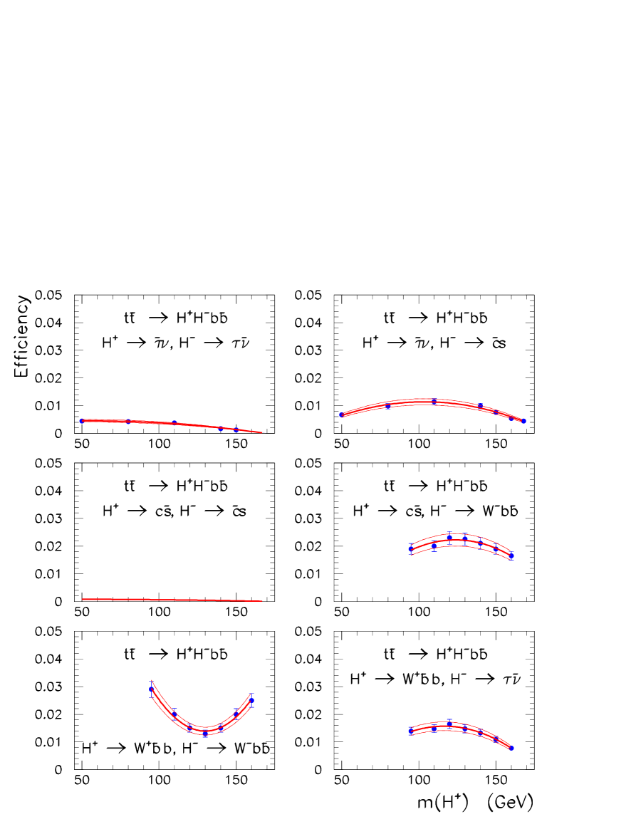
It is easy to see why the efficiencies are low in regions of parameter space dominated by (small , small ). When both top quarks decay to charged Higgs, and both charged Higgs decay to , there is no legitimate source for an isolated or , nor for large , in the final state. Compared to the SM, efficiencies are lower in regions dominated by (large ) because leptons decay hadronically most of the time, and a veto is applied to events containing s. Even when a from an decays to an or a , the lepton usually has a lower compared to one from a prompt decay of a . Regions dominated by (small , large ) are more difficult to discriminate against because real bosons are produced. However, such events are characterized by a large number of jets (up to 6), and can be suppressed somewhat by requiring that no more than two of the jets be tagged as .


Likelihood analysis
For observed events, the joint posterior probability density for and is given by
| (80) |
where , is the Poisson probability of observing events, given a total (signal + background) expectation of
| (81) |
and represents a Gaussian distribution. The means and widths of the Gaussians for the integrated luminosity , and the number of background events , are given in Table 50, while those for the acceptance , are calculated using Eq. (79), with parametrized functions for , and leading order calculations of , .
| Integrated luminosity, | fb |
|---|---|
| Estimated background, | |
| Expected signal (SM), | 24 |
Equation (80), which we parametrize as a function of and , gives a Bayesian posterior probability density for those parameters Jaynes . The prior distribution is assumed to be uniform in and in . Assuming instead that the prior is uniform in and in does not significantly alter the posterior distribution. To calculate probabilities, a Monte Carlo integration is carried out by spanning the parameter space in steps of 5 GeV in from 50 GeV to 160 GeV, with 25 uniform steps in covering the range at each value of , and performing 400,000 trials of Eq. (80) at each step.
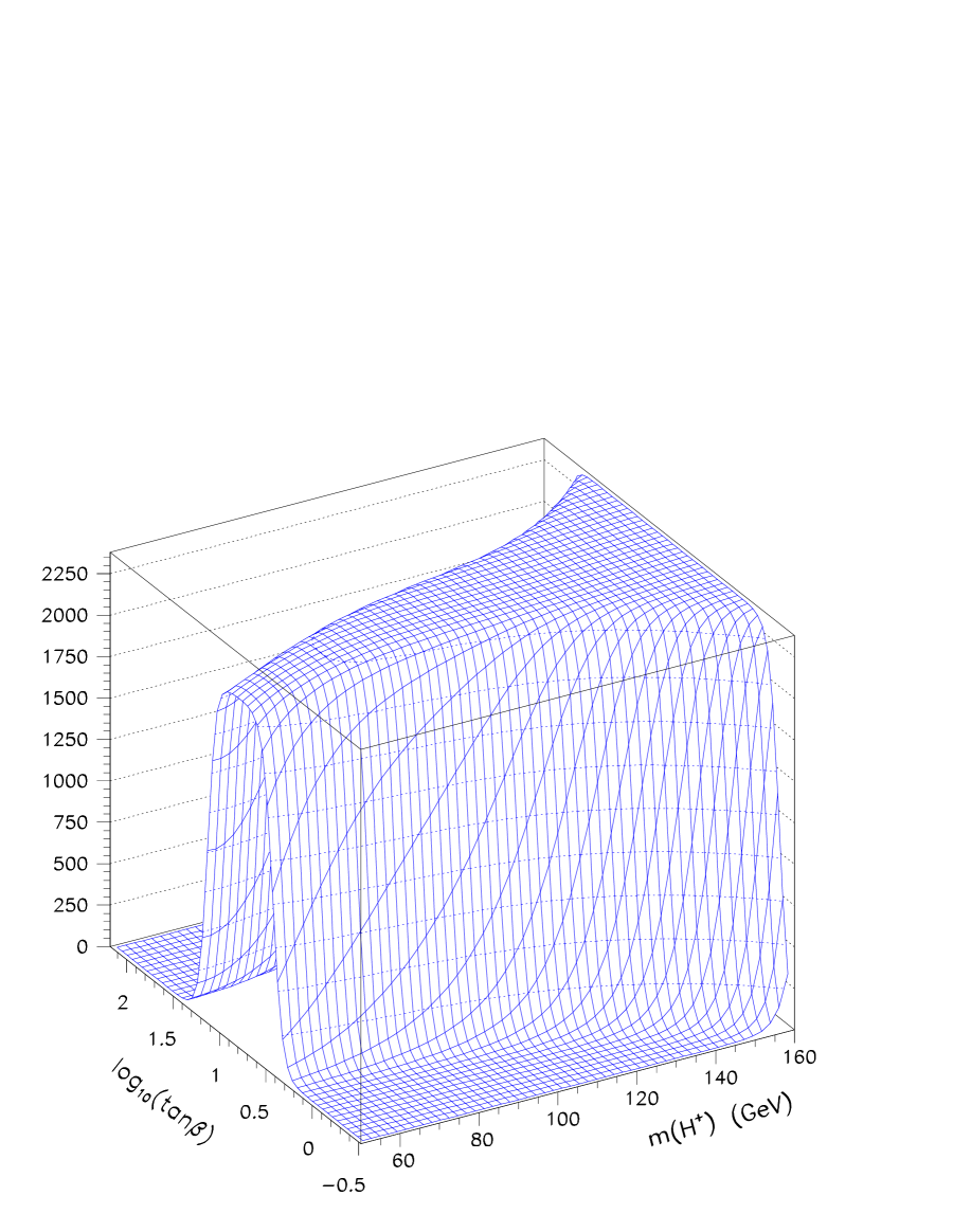
The likelihood predicted by the SM for observing events is shown in Fig. 99, while Fig. 100 shows the posterior probability density for corresponding to several values of for = 80 GeV. For a given value of , the 95% CL exclusion boundary in the [] plane is obtained by integrating the probability density , given by Eq. (80), between contours of constant . The likelihood surface corresponding to the parameters given in Table 50, and = 600, is shown in Fig. 102 for three different values of : 109 pb-1 (Run 1, TeV TEV ), 2 fb-1, and 10 fb-1.

Conclusions
Our study shows that, compared to Run 1 TEV , the search for charged Higgs bosons in decays of pair-produced top quarks will have a much greater reach in Run 2. A direct appearance search for charged Higgs bosons in decays of top quark is also possible. At the Tevatron, it would primarily involve a search for , which limits its applicability to . CDF has published results from such searches based on Run 1 data CDFch ; CDF_H+_2 which are consistent with its disappearance search results. Comparable results from an appearance search performed by DØ are expected soon. An appearance search in the region of will have to be based on . This will be more challenging since and quarks are more difficult to identify than s and s. However, if is substantially larger than , then it may be possible to distinguish (, ) from (, ) based on event kinematics. The indirect disappearance search presented here is expected to yield stronger null results than a direct appearance search for integrated luminosities up to 2–4 fb-1. If there is a charged Higgs lighter than the top quark, its presence can be detected by a disappearance search if is substantially different from , prompting a direct search to confirm discovery. Beyond Run 2, appearance searches should lead to superior results.
III Interpretation
III.1 Combined Standard Model Higgs Boson Results
J. Conway
As the results of Section II show, there is no single search channel for the Higgs which one might call “golden”; to maximize the sensitivity of the Higgs search it is necessary to combine the results of all the channels. This section presents the results of combining all Standard Model Higgs search channels, from both experiments, in terms of the integrated luminosity needed to exclude the Higgs at 95% CL (assuming it is not there) or discover it at the or level if it is.
Statistical Method \\
The statistical method employed here for combining channels is discussed in the Appendix. Briefly, the result of each search channel is treated as a counting experiment, and for a given outcome there is some Poisson probability. For all channels in both experiments, these probabilities are multiplied together to form a joint likelihood. This likelihood can be expressed as a function of the Higgs signal cross section, and can be used to set 95% CL limits or discovery significances. To take into account all possible experimental outcomes, the integrated luminosity threshold quoted below represent those values for which the desired statistical threshold is met in 50% of all possible outcomes.
Overview of results \\
The results of all the channels studied are summarized in Tables 51 and 52. The tables show the expected signal , the expected background , and the sensitivity in each channel as a function of the assumed Higgs mass. In all the low-mass channels, we have taken the numbers from assuming a 10% resolution in .
The tables indicate that of the low mass channels, the and have the most sensitivity. Also, while the dilepton mode adds significantly to the sensitivity, the all-hadronic channel brings little information to the final combination.
In comparing the different analyses, it is clear that the neural network technique results in significantly enhanced sensitivity in the three channels where it has been studied. Note that the NN- and SHW-based channel analyses do not take into account trigger inefficiency for events which otherwise pass the selection; this should be no problem in the and cases but may be a slight overestimate at low masses in the case.
For the high-mass channels, the channel has the most sensitivity, whereas the channel has nearly as good sensitivity over a broader mass range.
| Higgs Mass (GeV/) | ||||||
| Channel | Rate | 90 | 100 | 110 | 120 | 130 |
| 8.4 | 6.6 | 5.0 | 3.7 | 2.2 | ||
| (CDF) | 48 | 52 | 48 | 49 | 42 | |
| 1.2 | 0.9 | 0.7 | 0.5 | 0.3 | ||
| 10 | 8 | 5 | 4 | 3 | ||
| (SHW) | 75 | 68 | 57 | 58 | 52 | |
| 1.1 | 1.0 | 0.7 | 0.5 | 0.4 | ||
| 8.7 | 9.0 | 4.8 | 4.4 | 3.7 | ||
| (NN) | 28 | 39 | 19 | 26 | 46 | |
| 1.6 | 1.4 | 1.1 | 0.9 | 0.5 | ||
| 2.5 | 2.2 | 1.9 | 1.2 | 0.6 | ||
| (CDF) | 20.0 | 18.6 | 16.0 | 13.0 | 9.6 | |
| 0.6 | 0.5 | 0.5 | 0.3 | 0.2 | ||
| 8.9 | 6.7 | 4.6 | 3.2 | 2.1 | ||
| (SHW) | 77 | 69 | 56 | 39 | 30 | |
| 1.0 | 0.8 | 0.6 | 0.5 | 0.4 | ||
| 12 | 8 | 6.3 | 4.7 | 3.9 | ||
| (NN) | 123 | 70 | 55 | 45 | 47 | |
| 1.1 | 1.0 | 0.8 | 0.7 | 0.6 | ||
| 1.0 | 0.9 | 0.8 | 0.5 | 0.3 | ||
| (CDF) | 3.6 | 3.1 | 2.5 | 1.8 | 1.1 | |
| 0.5 | 0.5 | 0.5 | 0.4 | 0.3 | ||
| 1.5 | 1.2 | 0.9 | 0.6 | 0.4 | ||
| (SHW) | 4.9 | 4.3 | 3.2 | 2.3 | 1.9 | |
| 0.7 | 0.6 | 0.5 | 0.4 | 0.3 | ||
| 1.2 | 0.9 | 0.8 | 0.8 | 0.6 | ||
| (NN) | 2.9 | 1.9 | 2.3 | 2.8 | 1.9 | |
| 0.7 | 0.7 | 0.5 | 0.5 | 0.4 | ||
| 8.1 | 5.6 | 3.5 | 2.5 | 1.3 | ||
| (SHW) | 6800 | 3600 | 2800 | 2300 | 2000 | |
| 0.10 | 0.09 | 0.07 | 0.05 | 0.03 | ||
| Higgs Mass (GeV/) | ||||||||
|---|---|---|---|---|---|---|---|---|
| Channel | Rate | 120 | 130 | 140 | 150 | 160 | 170 | 180 |
| - | - | 2.6 | 2.8 | 1.5 | 1.1 | 1.0 | ||
| - | - | 44 | 30 | 4.4 | 2.4 | 3.8 | ||
| - | - | 0.39 | 0.51 | 0.71 | 0.71 | 0.51 | ||
| 0.08 | 0.15 | 0.29 | 0.36 | 0.41 | 0.38 | 0.26 | ||
| 0.58 | 0.58 | 0.58 | 0.58 | 0.58 | 0.58 | 0.58 | ||
| 0.11 | 0.20 | 0.38 | 0.47 | 0.54 | 0.50 | 0.34 | ||
Combined channel integrated luminosity thresholds \\
We perform determinations of the integrated luminosity thresholds combining all low-mass and high-mass channels. In the combination we assume that both experiments’ data is used by doubling each channel: we generate separate pseudoexperimental outcomes for each channel in each experiment, and combine all the results together in the final likelihood.
To take into account reasonable systematic errors, we incorporate into the likelihood a relative uncertainty on the background for each channel which is the smaller of 10% of the expected background or , where is the integrated luminosity and is the expected number of background events in 1 fb-1. Such an assumption is typical of the level of uncertainty experienced in new particle searches at the Tevatron. Note that if one does not let the systematic error decrease with integrated luminosity, numerical instability can result. More importantly, in the real experiments as the integrated luminosity increases the experimenters will have better control of the systematic errors, and will in all likelihood harden the selection criteria to improve the sensitivity while maintaining tolerable systematic uncertainties. Without the inclusion of these systematic errors, the integrated luminosity thresholds are approximately 30-50% smaller.
Reliability of the results \\
The nature of a study like this is such that the final results (here the integrated luminosity thresholds) depend on several unknown performance factors. The main factors affecting the result of this study, in particular the results in the low-mass channels, are
-
•
the -tagging efficiency,
-
•
the mass resolution, and
-
•
the backgrounds in the various channels.
All the low mass channels require two -tagged jets, which makes the result very sensitive to this efficiency. The signal efficiency increases as the square of the -tag efficiency, whereas only the , , and QCD dijet backgrounds follow the same dependence. In the gaussian limit, the integrated luminosity thresholds scale with , so even if the backgrounds are dominated by real , increasing the tag efficiency by 10% for example while maintaining the mistag rate would result in a 20% reduction in the required integrated luminosity threshold.
Both CDF and DØ will have excellent vertex tracking, and new algorithms and solid understanding of vertex tracking systematics could result in efficiencies somewhat higher than assumed in this report. However, physics effects such as multiple interactions, and/or unforeseen detector performance issues could adversely affect the tag efficiency and purity. The assumptions made here are reasonably conservative.
The mass resolution is directly related to the background - indeed the main effect of improving the resolution is of course to reduce the number of background events in the window around the Higgs mass. As noted above, since the integrated luminosity thresholds scale with , increasing the background (or worsening the resolution) by some relative amount has a the same relative effect on the thresholds.
As the careful reader will note, in the channel analyses no estimates were made of the generic dijet background. This process has a very large cross section but tiny acceptance, and is thus not modeled reliably. In the CDF Run 1 analysis, this background was about half of the total, and estimated from the data. With better understanding, this fraction could potentially be reduced. However, we conservatively assume in the final combination that this background is equal to the rest of the background, that is, half of the total. This is reflected in Table 51 by doubling the non-dijet background in the channel analyses.
Perhaps of more concern is the assumption regarding the mass resolution ultimately attainable. In the low mass region this has been assumed to be 10% (of the Higgs mass). Even with a perfect detector the physics of the jet fragmentation and gluon radiation, along with the missing neutrinos from the quark decay limit the mass resolution attainable to a lineshape with a width of about 8% with a tail on the low side. If detector-related effects can be understood and controlled well, and if all the available detector information is brought to bear, the estimate of 10% may be reasonable. Even if the mass resolution is closer to 12%, though, the resulting integrated luminosity thresholds will only be 20% larger, well within the other uncertainties inherent in this work.
Furthermore, at this level the relative strengths and weaknesses of the two detectors will ultimately determine the sensitivity to the Higgs. With more elaborate tracking, CDF will most likely excel in terms of tagging efficiency, whereas with its more hermetic calorimeter the DØ experiment may attain the best mass resolution.
Given the above discussion, the basic conclusions arrived at below are not unreasonably aggressive. Breakthroughs in technique are always possible, and have indeed been the norm in the past. For example both the Higgs search in LEP1 and the top quark search in Run 1 at the Tevatron exceeded the expectations of studies prior to machine turn-on. The studies presented here should be taken as cautiously optimistic: Using full mass spectrum fits, applying neural network techniques, improving the trigger efficiencies, adding other search mode, and improving the mass resolution and tagging efficiency beyond that projected here may all serve to dramatically improve the discovery potential for the Higgs at the Tevatron.
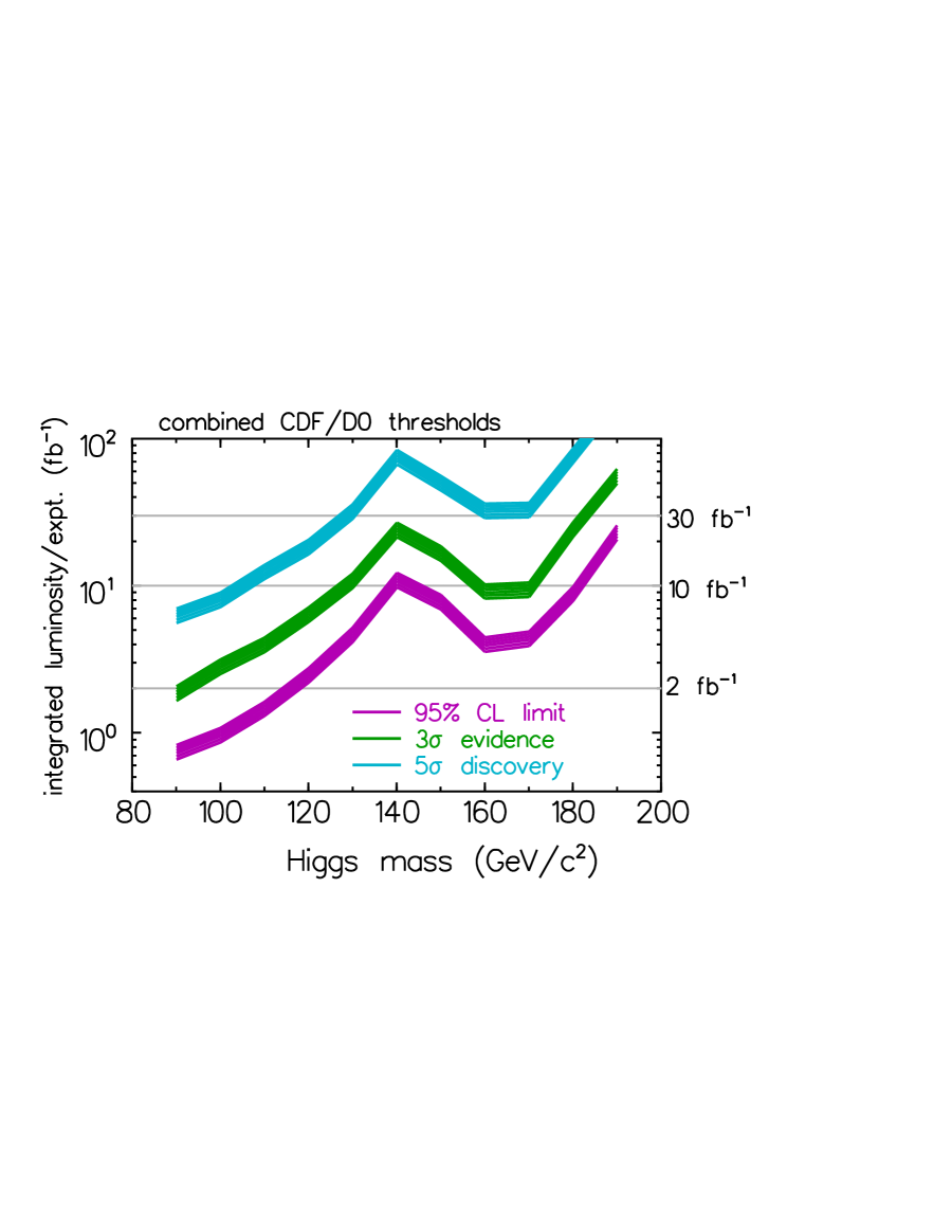
Combined channel integrated luminosity thresholds \\
Fig. 103 shows the integrated luminosity required to either exclude the SM Higgs boson at 95% CL or discover it at the or level of significance, as a function of Higgs mass, for the SHW analyses with the neural net selection. The integrated luminosity displayed in the plot is the delivered integrated luminosity per experiment; whereas the shaded bands shown are the results obtained by combining the statistical power of both experiments. The required integrated luminosity thresholds for a single experiment are very close to a factor of two higher than those for the two combined experiments. The bands extend from the calculated threshold on the low side upward in required integrated luminosity by 30% to the high side, as an indication of the range of uncertainty in the various factors discussed above. As the plots show, the required integrated luminosity increases rapidly with Higgs mass to 140 GeV, beyond which the high-mass channels play the dominant role. At the upgraded Tevatron with 2 fb-1 per detector, the 95% CL limits will barely extend the expected LEP2 limits, but with 10 fb-1, the SM Higgs boson can be excluded up to 180 GeV in the absence of a Higgs signal.
If a SM Higgs boson exists with mass less than 180 GeV, the combined sensitivity of CDF and DØ will yield evidence for the Higgs boson at the level with 20 fb-1. (The Higgs mass region around 140 GeV may require slightly more luminosity depending on the magnitude of systematic errors due to uncertainties in -tagging efficiency, background rate, the mass resolution, etc.) With 30 fb-1 integrated luminosity delivered per detector, a Higgs boson discovery may be possible for Higgs masses up to about 130 GeV, a significant extension of the LEP2 Standard Model Higgs search. The latter figure of merit is particularly significant when applied to the search for the lightest Higgs bosons of the minimal supersymmetric model. We address this case in detail in the following section.
III.2 Higgs Mass Reach in Low-Energy Supersymmetry
M. Carena, H.E. Haber, S. Mrenna and C.E.M. Wagner
III.2.1 Reinterpretation of the Standard Model Analysis in Extended Higgs Sector Theories
The Standard Model Higgs boson search simulations presented in this report can be interpreted more generally in the framework of an extended Higgs sector. Generically, extended Higgs sectors contain additional scalar states beyond with different couplings from those found in the Standard Model. The Higgs boson search strategies of Sections II.C and II.D can be applied to a CP-even neutral Higgs boson, and those of Section II.F to both CP-even and CP-odd neutral Higgs bosons. If CP is not conserved, then the neutral scalar states can be considered to be mixtures of CP-even and CP-odd scalars, and the discussion that follows must be modified accordingly cpcarlos ; cpcarlos2 . Charged Higgs boson states may also be present; the corresponding search strategies were discussed in Section II.G. Finally, signatures not considered in this report are also possible, such as the associated production of CP-even and CP-odd neutral scalars and Higgs boson decays into leptons. These additional signatures deserve a closer examination and might improve the Higgs discovery reach beyond the results given in this section.
Before considering specific extensions of the Higgs sector, it is useful to express the Standard Model results in a more model-independent fashion. We focus on the analyses based on Higgs processes in which the production and decay depend primarily on a single Higgs boson coupling. To simplify the presentation, several fixed values of integrated luminosity ( fb-1) were chosen as well as two statistical measures (95% Confidence Level exclusion, 5 discovery) for the significance of a Higgs boson signal.
As a function of the Higgs boson mass, the experimental sensitivity can be described by the ratio of the chosen level of statistical significance and the actual statistical significance for a fixed value of integrated luminosity. This ratio is denoted by and depends on the assumed integrated luminosity,474747Following the conventions of this report, the integrated luminosity is taken to be per experiment, corresponding to the total luminosity delivered to the collider. All plots shown in this section assume that equal data sets from the CDF and DØ detectors are combined. the chosen statistical measure and the Higgs boson mass. For example, if the discovery criterion is , and the expected significance of a Standard Model Higgs boson with mass 125 GeV is with 10 fb-1 of data, then at 125 GeV. This means that a 125 GeV Higgs boson from some extended Higgs sector could be discovered with 10 fb-1 of data if the production cross section times branching ratio were 1.5 times the Standard Model value. Alternatively, times more data is required for a discovery of a Standard Model Higgs boson at this mass (in the limit of Gaussian statistics, for a background limited measurement, when the significance scales as the square-root of integrated luminosity).
Once the -values are obtained, they can be applied to a particular model of an extended Higgs sector. For a given extended Higgs model, a theoretical value at a fixed can be computed for the set of parameters that define the model. The Higgs mass, , may be one of the defining input parameters of the extended Higgs model. To be more precise, at a fixed Higgs boson mass, for a given Higgs boson production process (e.g., or ) with the subsequent decay , we define
| (82) |
where the numerator corresponds to the Higgs cross section times branching ratio predicted in the extended Higgs sector model, and the denominator corresponds to the same quantity in the Standard Model. If the theoretical value lies below for a particular , then there is no experimental sensitivity to this point of the model parameter space for the assumed luminosity and statistical significance. Clearly, if =1, then the Higgs mass reach is precisely that of the Standard Model, whereas if [] the corresponding Higgs boson mass reach is increased [decreased] with respect to that of the Standard Model.
Consider first the production of a neutral scalar, , in association with a vector boson ( or ), where . For the Tevatron Standard Model Higgs search, this mechanism is relevant in the mass range GeV. In this case, the Higgs search simulations of Sections II.C.1–4 apply. The resulting -curves corresponding to a 95 CL exclusion and discovery at the 5 level are shown in fig. 104.
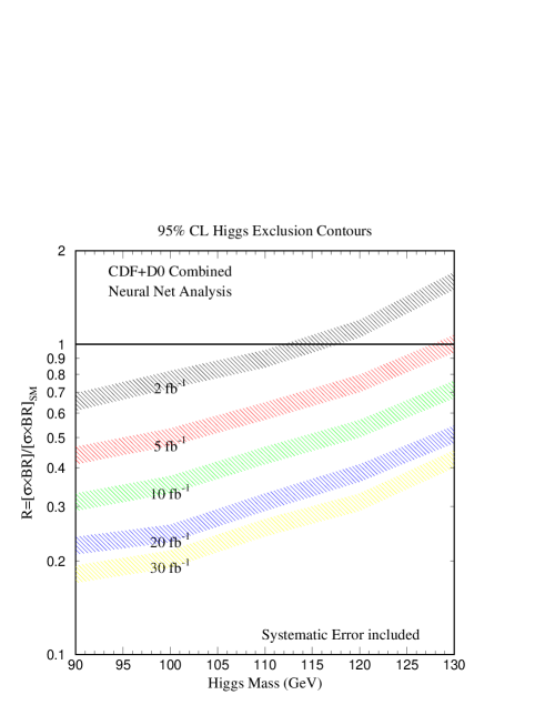
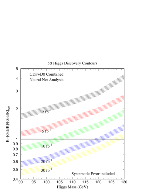
The cross section is governed by the coupling ,484848It is assumed that the ratio of and couplings is the same as in the Standard Model. This assumption is correct in multi-doublet Higgs models, but can be violated in models with higher Higgs representations wudka . while the rate for the observed final state (, where decays leptonically) depends on the branching ratio of . The relevant -curves are obtained by taking and in eq. (82):
| (83) |
These curves will be used in the next section to examine the Higgs mass reach of the upgraded Tevatron in the framework of the MSSM.
In the Higgs boson mass range of GeV, the main Tevatron discovery signature for a Standard Model Higgs boson comes from two channels: (where both ’s decay leptonically) and [ or ] (where two of the three vector bosons decay leptonically and the third decays hadronically; the same-sign dilepton final states provide the largest statistical weight). The two production mechanisms depend upon different Higgs boson couplings and are treated separately. The simulations of Section II.D are used to obtain the separate -curves shown in figs. 105 and 106. Separate theoretical -curves are defined for cases and :
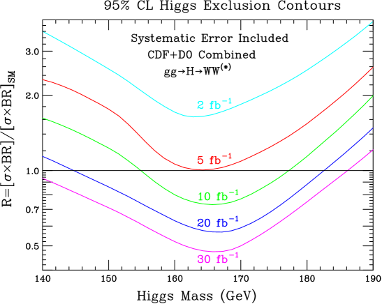
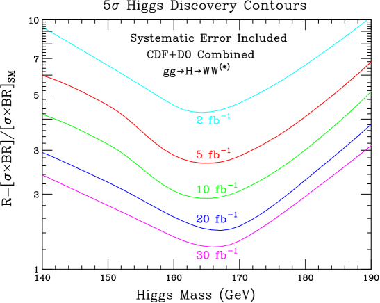
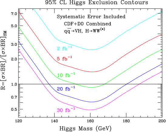
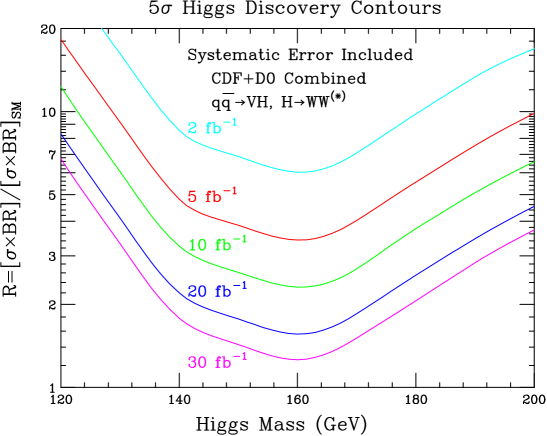
Clearly, a combination of both channels and yields the maximal sensitivity for Higgs discovery reach (or exclusion). However, this must be done on a model-by-model basis, since different couplings may be involved in the calculation of the two values in any given extension of the Standard Model. Note that in the MSSM, the coupling is significantly suppressed for GeV (in this mass range, is the heavier CP-even Higgs boson, ). Thus, in the MSSM, the predicted values of and are substantially smaller than 1.494949 is suppressed [enhanced] relative to the Standard Model for moderate [large] values of . But, at large , the suppression of is more significant than the enhancement of the rate, resulting in . As a result, the high mass Tevatron Standard Model Higgs search has no relevance for the MSSM analysis, and it will not be employed in the next section. In models of extended Higgs sectors with exotic Higgs representations, parameter ranges in which and/or are larger than one can occur. As an extreme example, models of non-minimal Higgs sectors have been constructed in which the tree-level coupling of the Higgs bosons to fermions is absent (or highly suppressed). In such “fermiophobic” Higgs models fermiophobe , the Higgs coupling to gluons (which normally occurs at one-loop via the fermion loop graph) is approximately zero and vanishes.
The last search channel considered here is Higgs production via , , followed by the decay . The ratio is defined using eq. (82) with and . Since is proportional to the square of the Yukawa coupling, , it follows that:
| (84) |
The resulting curves corresponding to a 95 CL Higgs mass exclusion and Higgs discovery at the 5 level, based on the CDF and DØ analyses of Section II.F, are shown in fig. 107. Note that the DØ analysis has greater sensitivity at large values of than the CDF analysis, whereas the CDF analysis has greater sensitivity at low values of . The case of Standard Model Higgs boson production, , would correspond to in fig. 107. Clearly, neither analysis shows any sensitivity to the production of a Standard Model Higgs boson in the channel for any reasonable luminosity.
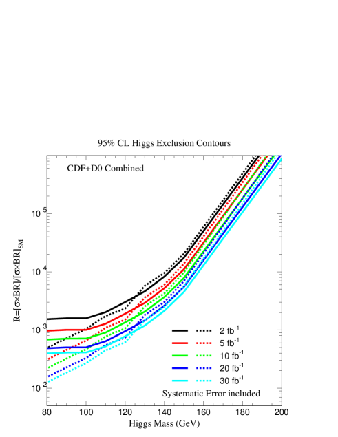
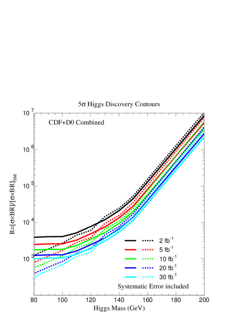
Although the values of must be quite large in order to have any sensitivity to the channel, such enhancements can readily occur in extensions of the Standard Model. The main limitation of the SM searches in this channel, is that is greatly suppressed once 135 GeV and decays to W or Z boson pairs become important. In the MSSM at large , can be significantly enhanced. In Section I.C.1 [below eq. (I.3.1)], we showed that the tree-level coupling is enhanced (relative to the Standard Model value) by a factor of for either , or , (depending on the value of ). Evaluating eq. (84) for the case where is one of the neutral Higgs bosons with an enhanced coupling to , and taking , one finds 505050The value of can be modified at large in some regions of the MSSM parameter space.
| (85) |
Since for GeV, and sensible parameter regimes exist where is possible, there is sensitivity to the channel for an interesting range of Higgs masses and for integrated luminosities as low as 2. This will be discussed further in Section III.B.3. Whereas the -curves in fig. 107 are based on the production of a CP-even neutral scalar, they also apply to the CP-odd Higgs boson, because the corresponding cross-section and decay branching ratios are very similar [see figs. 13 and 15]. Thus, one can reliably employ the -curves obtained above to production in the MSSM.
III.2.2 MSSM Higgs Sector Results: [, ],
The general MSSM parameter space involves many a priori unknown parameters. In practice, only a small subset of these parameters govern the properties of the Higgs sector. A full scan of this reduced subset is a formidable task. However, a detailed study of a few appropriately chosen points of the parameter space can help determine the ultimate MSSM Higgs discovery reach of the upgraded Tevatron.
In order to select a representative set of parameters, it is useful to study approximate analytic expressions for the elements of the CP-even Higgs boson squared-mass matrix. At tree-level, all MSSM Higgs masses and couplings are functions of and . As shown in Section I.C.2 and I.C.3, the radiative corrections to Higgs masses and couplings depend primarily on the third generation squark mass and mixing parameters (with a somewhat weaker dependence on the gluino mass). In the “generic” MSSM analysis, we derive exclusion and discovery regions in the – plane for various benchmark values of these parameters.
In the generic MSSM analysis, all the relevant MSSM parameters that govern the Higgs sector masses and couplings are regarded as independent. These parameters arise primarily from the supersymmetry-breaking sector of the theory. However, there is no underlying theoretical model of supersymmetry-breaking that yields precisely the set of benchmark parameters that we have employed in the generic MSSM analysis. An alternative approach is to choose a specific model of supersymmetry-breaking, and then derive the values of the relevant supersymmetric parameters (as a function of more fundamental model parameters). We shall illustrate this procedure in the minimal supergravity (mSUGRA) model and in simple models of gauge-mediated supersymmetry-breaking.
a. Generic MSSM Analysis \\[0.2cm]
The results of Sections II.C.1–4, based on the SHW simulation improved by neural network techniques, show that a Standard Model Higgs boson with GeV can be excluded at the 95% CL [discovered at the 5 level] for an integrated luminosity of 5 fb-1 [30 fb-1]. In Section I.C.2, it was noted that there is an upper bound to the value of the lightest CP-even neutral Higgs boson, , of the MSSM. Assuming an average squark mass parameter of TeV, then GeV. This suggests that a significant region of the MSSM parameter space can be probed by the Tevatron Higgs search with enough integrated luminosity. This can be understood by considering limiting cases of the MSSM in which some or all of the properties of one of the neutral CP-even Higgs bosons approach those of . For example, the limit corresponds to the case in which the heavy CP-even, the CP-odd and the charged Higgs decouple from the low energy effective theory and . In this “decoupling” region of MSSM parameter space, the Standard Model simulations apply directly. Other regions of MSSM parameter space exist in which behaves in part like a Standard Model Higgs boson. As discussed in Section I.C.2, in the region of and , one finds that GeV and the coupling of to pairs is nearly equal to the corresponding coupling. As long as is not significantly suppressed, the Standard Model Higgs simulation can be applied to in this MSSM parameter regime.
In the rest of the MSSM parameter space, both and couplings to vector bosons and fermions differ from those of . For the generic MSSM analysis, [, ] is computed as a function of and . Applying eq. (82) to the MSSM yields
The above equations demonstrate the complementarity of the and channels in the coverage of the – plane coming from the dependence on and of the ratio of MSSM to SM cross sections in each case. The ratio of branching ratios has a more complicated behavior as a function of the supersymmetric parameters. In a large region of the MSSM parameter space,515151This is especially true in the region of large where [ or depending on ] may be enhanced relative to the Standard Model. with [, ] is slightly above 1 (over the Higgs mass range of interest). Thus, may be slightly above 1 if [for ] or [for ]. In contrast, in the region where , the values for both and are significantly below 1, which severely limits the sensitivity of the Tevatron Higgs search. Finally, small regions of MSSM parameter space exist (as discussed in Section I.C.3), in which [ or ] is strongly suppressed relative to the Standard Model, even though is near the Standard Model value. In these regions, and the channel is not a promising search mode.
Once the values of the squark mass and mixing parameters are fixed, the two ratios [ and ] can be computed as a function of and . If the value is larger than at the same in fig. 104(a) (for a given integrated luminosity), then this point of parameter space can be excluded at the 95% CL. If is larger than at the same in fig. 104(b), then can be discovered at the 5 level. Whereas in most of the – plane, either or is the relevant Higgs boson, there are some regions of MSSM parameter space where where both Higgs bosons have comparable rates. If GeV, then the individual values of the and signals are added in quadrature before comparing to . This procedure is meant to crudely represent the fact that the two signals will add constructively as long as the mass difference is within the experimental resolution.525252One would expect some loss of significance, depending on the actual mass splitting, since some of the signal will leak out of the a priori chosen mass window. Note that the near degeneracy of and occurs only in the narrow region of MSSM parameter space when .
| Mass parameters [TeV] | (GeV) | |||||
|---|---|---|---|---|---|---|
| Benchmark | ||||||
| maximal mixing | 1.0 | 1.0 | 129 | |||
| no-mixing | 1.0 | 1.0 | 115 | |||
| suppressed production | 1.5 | 0 | 1.0 | 1.0 | 120 | |
Table 53 defines the set of benchmark parameters for the relevant supersymmetric parameters that govern the Higgs radiative corrections. These include the supersymmetric Higgs mass parameter , the third generation squark mixing parameters, and , the gluino mass , and the diagonal soft-supersymmetry-breaking third generation squark squared-masses (which we take for simplicity to be degenerate and equal to ). The maximal mixing benchmark scenario, as the name suggests, is defined as the one in which the squark mixing parameters are such that they maximize the value of the lightest CP-even Higgs boson mass for fixed values of , and . In contrast, in the no-mixing scenario, the parameters and are chosen such that the combination vanishes. In this limit, the value of the lightest CP-even Higgs boson is at its minimum for fixed values of , and . This corresponds to the minimal mixing case studied in Section I.C.2. [See fig. 7 for the dependence of on the squark mixing parameter .]
One might conclude that the maximal mixing scenario, in which can attain its maximal value for a given set of MSSM parameters, is the most conservative case for ascertaining the Higgs mass discovery reach of the upgraded Tevatron. However, a scan through the MSSM parameters away from the maximal squark mixing point reveals regions of parameter space in which the CP-even neutral Higgs boson with Standard-Model-like couplings to has suppressed couplings to . The benchmark scenario denoted by “suppressed production” in table 53 is an example of this behavior. The regions of strongly suppressed correspond to a suppressed coupling at lower and a suppressed coupling at larger . In particular, the suppression for large extends to relatively large values of , indicating a delay in the onset of the decoupling limit (where the coupling approaches the Standard Model value). This is the case when one of the Higgs bosons becomes mostly , with no coupling to down-type quarks except those induced by supersymmetry-breaking effects [see eq. (28)]. Such a Higgs boson has SM–like couplings to the and , but vanishing couplings to and . The necessary condition for this limit to arise is explained in Section I.C.3. In fact, in the suppressed benchmark scenario, all the Higgs couplings to are generally suppressed, since and [see eqs. (35), (37) and (38)]. From the analytic formulae, it can be deduced that and large values of , and are needed.
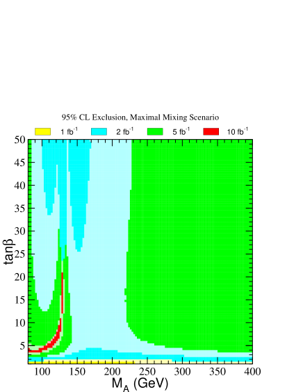
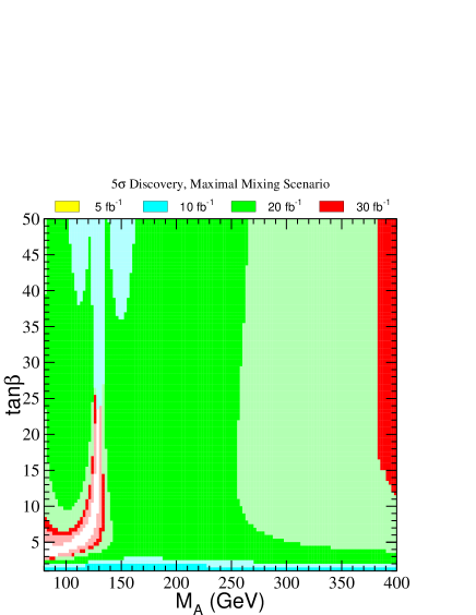
Fig. 108 shows contour plots demonstrating regions of 95 exclusion and discovery for the maximal mixing benchmark scenario as defined in table 53. This illustrates more generally the fact that the MSSM parameter space coverage in the channel depends sensitively on the maximal value of the lightest Higgs boson mass for a particular set of MSSM parameters. The darker shading of a given color illustrates how a net reduction in the detection efficiency, due to the uncertainties in -tagging efficiency, background, mass resolution and other effects, translates in a the coverage of the MSSM – plane.
A closer examination of fig. 108 shows three regions of the MSSM parameter space that raise difficulties for the Tevatron search. In the region of large and (where ), the coupling is highly suppressed, so that is the relevant process. For large and large the incomplete parameter space coverage is simply due to the fact that the lightest Higgs has SM like couplings and its mass is at the maximal value. Another problematical region of MSSM parameter space corresponds to the case of and moderate , where . If is sufficiently large, the two CP–even Higgs bosons tend to have similar masses, and both states contribute to the Higgs signal in the same mass bin. However, a hole in the coverage of the vs. plane persists in a small region for between 5 and 20, since in this case the mass difference is large and . In contrast, a signal can be observed with less integrated luminosity in the region of GeV, since and the coupling is strongly enhanced with respect to the Standard Model case, implying an increase in the branching ratio of this Higgs boson into bottom quarks.
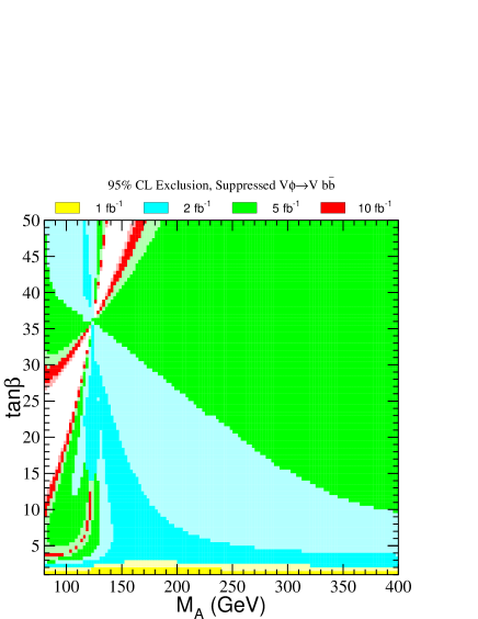
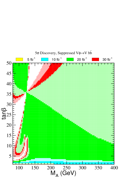
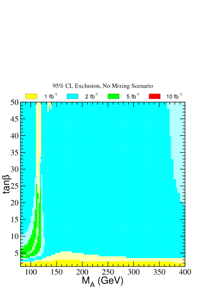
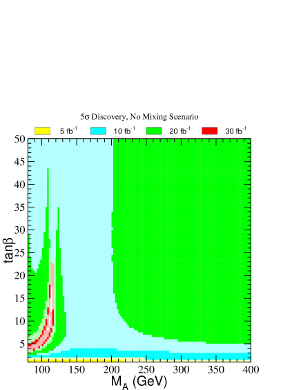
Fig. 109 illustrates the effect of the suppressed couplings for the Tevatron MSSM Higgs search for the “suppressed ” benchmark scenario of table 53. The small hole in the coverage of the vs. plane for between 5 and 15 corresponds to the same difficult region of MSSM parameter space noted in the maximal mixing case above. However, in the present case, two new larger holes open up corresponding to the regions of strongly suppressed coupling noted above. Since in this case one has 0, there is a suppression of the coupling via a suppression of the radiatively corrected value of . On the other hand, although the gluino mass and are large, the vertex corrections to the bottom Yukawa coupling have the effect of suppressing the coupling, since 0 and, hence, is also positive. Again, as explained above, the darker shading of a given color shows the uncertainty in the discovery and exclusion potential due to uncertainties in the experimental simulations.
Fig. 110 shows contours of discovery and 95% CL exclusion for the case of the “no-mixing” benchmark scenario defined in table 53, which yields the smallest value for the mass of the Higgs boson that has SM–like couplings to the and bosons as a function of the squark mixing effects. This is an optimistic scenario for the Tevatron, in which only modest values of integrated luminosity are necessary to cover a significant portion of the – plane. Note, however, that the maximal mass for the lightest Higgs boson is about 115 GeV. Much of this parameter regime will have been probed at LEP by the end of its final run.
b. Model-Dependent MSSM Analysis
H. Baer, B.W. Harris and X. Tata
The Higgs sector masses and couplings are determined from a set of soft-supersymmetry-breaking parameters that include three gaugino mass parameters, scalar squared-mass parameters for squarks, sleptons and Higgs bosons, the parameters that govern cubic scalar interactions, and the parameter that mixes the two Higgs scalars. In addition, there is also dependence on the supersymmetric Higgsino mass parameter . The latter two parameters can be exchanged for the two Higgs vacuum expectation values, under the assumption that the electroweak symmetry is broken in the usual manner. The origin of the soft-supersymmetry-breaking parameters is not presently known. Nevertheless, one may consider specific models of supersymmetry breaking, where the soft-supersymmetry-breaking parameters are specified. In such approaches, one often makes simplifying assumptions in order to reduce the total number of free parameters. Although such assumptions are ad-hoc, the resulting models do provide examples of how the soft-supersymmetry-breaking parameters could be correlated. The results of such correlations would constrain the Higgs sector of a generic MSSM. In particular, the discovery of the Higgs bosons of the MSSM would place interesting constraints on the underlying supersymmetric parameters.
In the minimal supergravity (mSUGRA) framework Nilles85 ; sugra ; sugrawork , the supersymmetry breaking takes place in a hidden sector, and supersymmetry-breaking effects are communicated to the observable sector via Planck-scale interactions. In the minimal rendition of this model the soft-supersymmetry-breaking parameters take a particularly simple form when evaluated at a very high energy scale (usually taken to be either the Planck scale or the grand unification scale). At this high-energy scale, all scalars have a common mass , all gauginos have a common mass , and all trilinear scalar couplings unify to . The low-energy Higgs and supersymmetric parameters that govern the observed Higgs and supersymmetric phenomenology are obtained via renormalization group running of soft-supersymmetry-breaking masses and couplings from the high-energy scale down to the electroweak scale. In a successful mSUGRA model, electroweak symmetry breaking is radiatively generated, since at least one of the Higgs squared-masses is driven negative in the renormalization-group evolution.
One can count the number of independent parameters in the mSUGRA framework. In addition to usual Standard Model parameters (excluding the Higgs mass), one must specify , , , and Planck-scale values for the and -parameters (denoted by and ). In principle, , and can be complex, although in the mSUGRA approach, these parameters are taken (arbitrarily) to be real. As previously noted, renormalization group evolution is used to compute the low-energy values of the mSUGRA parameters, which then fixes all the parameters of the low-energy MSSM. In particular, the two Higgs vacuum expectation values (or equivalently, and ) can be expressed as a function of the Planck-scale supergravity parameters. The simplest procedure is to express and in terms of the low-energy and parameters and the other free mSUGRA parameters (the sign of is not fixed in this process). The resulting MSSM spectrum and its interaction strengths are then determined by five parameters: , , , , and the sign of , in addition to the usual parameters of the Standard Model.
Recently, attention has been given to a class of supergravity models in which the common tree-level gaugino mass is absent. In such models, one finds a model-independent contribution to the gaugino mass anomalymed , whose origin can be traced to the super-conformal (super-Weyl) anomaly which is common to all supergravity models. This approach has been called anomaly-mediated supersymmetry breaking. In the simplest scenario, all supersymmetric particle masses are determined by one overall mass parameter (the gravitino mass, ). However, anomaly-mediation cannot be the sole source of supersymmetry-breaking in the MSSM (since in the simplest of such models, slepton squared-masses are negative). Moreover, one still needs a model for the origin of the and parameters in order to generate electroweak symmetry breaking and a realistic Higgs sector. One simple approach is to add to the theory a universal scalar mass parameter and and by hand. The resulting model depends on four parameters: , , and . A preliminary study of the Higgs boson discovery reach of the upgraded Tevatron in this scenario has been presented in ref. shufang .
In models of gauge-mediated supersymmetry breaking dine , supersymmetry breaking is transmitted to the MSSM via gauge forces. A typical structure of such models involves a hidden sector where supersymmetry is broken, a “messenger sector” consisting of particles (messengers) with SU(3)SU(2)U(1) quantum numbers, and the visible sector consisting of the fields of the MSSM gmsbreview . The direct coupling of the messengers to the hidden sector generates a supersymmetry breaking spectrum in the messenger sector. Finally, supersymmetry breaking is transmitted to the MSSM via the virtual exchange of the messengers.
In the gauge-mediated supersymmetry-breaking (GMSB) approach, the low-energy scalar and gaugino mass parameters are generated through loop-effects (while the resulting -parameters are suppressed). In minimal GMSB models, the supersymmetric particle masses are proportional to the parameter , where is the supersymmetry-breaking scale and the mass scale for the messenger particles. The origin of the and -parameters is model-dependent and lies somewhat outside the ansatz of gauge-mediated supersymmetry-breaking and must be taken to be additional free parameters. The minimal gauge-mediated (mGMSB) models of this type are parameterized in terms of , , , , and , where is the number of complete messenger multiplets ( if TeV to avoid the presence of Landau poles below ) and is the ratio of hidden sector to messenger sector vacuum expectation values of auxiliary fields pedro . As in the case of mSUGRA, one can re-express and in terms of and after the electroweak symmetry breaking conditions are imposed.
The mSUGRA and mGMSB models are incorporated in the event generator ISAJET ISAJET . The Higgs boson mass spectrum is obtained in ISAJET by minimizing the renormalization-group-improved one-loop effective potential. The minimization is performed at an optimized scale choice , which effectively includes the dominant two-loop contributions to the Higgs mass computations. The latest improvements including finite two loop effects through vertex corrections to the top and bottom Yukawa couplings are not taken into account in these analyses. Supersymmetric parameter values are used by ISAJET to calculate the various supersymmetric particle masses and mixing angles, and the Higgs boson masses and branching fractions bisset . The calculations presented here are an update of work previously presented in ref. bht .


The 95% exclusion and 5 discovery regions for the mSUGRA model are shown in fig. 112 for , and . The TH region is excluded either due to a lack of appropriate electroweak symmetry breaking, or because the lightest neutralino is not the lightest supersymmetric particle. The EX region is excluded by the negative results from LEP2 searches for chargino pair production, which require GeV. The LEP reach is shown here as indicative, assuming a maximal Higgs mass discovery potential of 108 GeV. For the region of mSUGRA parameters considered in fig. 112, the Fermilab Tevatron experiments should be able to explore the entire plane shown at 95% CL with 2 fb-1 or at with 20 fb-1.
The corresponding mSUGRA plots for are shown in fig. 112. In contrast to the small case just discussed, at large the mass of lies above the LEP2 reach. The Tevatron experiments should be able to probe the entire plane shown at 95% CL with 5 fb-1 of data. The discovery potential is more limited and requires an integrated luminosity as high as 30 fb-1 (for very large ) to ensure Higgs boson discovery.


The 95% exclusion and 5 discovery regions for the minimal gauge mediated supersymmetry breaking model, in the – plane, are shown in fig. 113, for and messenger scale GeV. The TH region is excluded due to a lack of appropriate electroweak symmetry breaking. The EX regions are excluded by experimental bounds on the mass of the lightest neutralino ( GeV). In these cases, the whole plane can be probed by Tevatron experiments at the 95% CL with 5 fb-1 of data. At the discovery level, the Tevatron experiments would need 20 fb-1 per experiment to be able to probe this model.
III.2.3 MSSM Higgs Sector Results: , [, , ]
In many extensions of the Standard Model (including the MSSM), there exists at least one non–Standard Model–like Higgs boson: its couplings to gauge bosons may vanish at tree–level or be suppressed through mixing, and their relative couplings to different fermions are not strictly set by the corresponding fermion masses. Such Higgs bosons will exist in models with many Higgs doublets when one of the doublets is mostly responsible for electroweak symmetry breaking. In the MSSM, the CP-odd scalar differs from the Standard Model Higgs boson, with enhanced couplings at large to down–type fermions and suppressed couplings to up–type ones. Additionally, when one of the CP-even Higgs bosons (either or ) has Standard Model–like couplings to the gauge bosons, the other one has a pattern of enhanced and suppressed couplings to fermions similar to that of the .
We consider the prospects for discovering such a non–Standard Model–like Higgs boson at the Tevatron, based on the signature studied in Section II.F. In the case of the MSSM, can in principle be one of three neutral Higgs bosons: , and . If is large, two of the Higgs bosons are produced with enhanced rates.535353As emphasized below eq. (I.3.1), at large the production rate of is enhanced for two of the neutral MSSM Higgs bosons: and [] if []. If these two Higgs bosons are very close in mass, then the corresponding signals should be added as they will not be distinguishable within the experimental resolution. However, over some range of and values, the two Higgs bosons with enhanced production rates are significantly split in mass. For example, for moderate values of , the corresponding mass splitting can be as much as – GeV, and the procedure for combining the signals must reflect this fact.
The previous considerations illustrate one of the limitations of encoding all the analysis information in a -curve. In some cases, knowledge of the signal size is also necessary. The expected signal in a given model is simply obtained by multiplying the Standard Model signal by the -value for the mass . Of course, the expected background in a mass window centered on the mass is unchanged by choosing a different model. The experimental sensitivity in the channel to a given set of MSSM parameters is estimated using the following algorithm. First, the CP even Higgs boson with the smallest value of is chosen as the non–Standard Model–like one. The expected signal for the CP even Higgs boson is calculated by multiplying the Standard Model signal by the -value for the CP-even Higgs boson, whereas the expected background in the mass window centered on the CP even Higgs boson mass is the same as in the Standard Model. The signal and background for is determined in a similar fashion.
The invariant mass distributions of the individual signals and are assumed to be well described by Gaussian distributions. To determine if the signals overlap, the mass splitting is compared to the quantity . The latter is the sum of two standard deviations in the invariant mass distribution of each signal assuming a mass resolution of 15%. If , then the two signals overlap within the experimental resolution. In this case, the mass window is expanded to contain both signals ( below the lightest Higgs boson mass and above the heavier one), and the number of background events within the window is calculated: . The systematic error on the background is assumed to be . This choice represents the Run 1 experience that systematic errors are roughly 10% of the number of background events, but also that the systematic errors do not increase without bound and tend to saturate at a level comparable to the statistical errors. The full error on the background, , is the quadrature of statistical and systematic errors, and the significance is defined as . If the two signals are well separated within the experimental resolution, then the significance of each signal is calculated separately: and . These two quantities are added in quadrature to determine the full significance. This algorithm is somewhat biased. For the case when both signals overlap (which coincides with the range of where the experiments might observe a signal), one must “know” that the best mass window is a larger one. It may be more realistic to choose the average Higgs boson mass as the center of the mass window of size .545454In the case when the signals do not overlap (which is not of practical interest since must be so small that the production cross section is highly suppressed), one should consider background fluctuations over all reasonable mass windows that do not overlap. Given the experimental resolution, and the maximal mass splitting possible, this is not a serious concern.
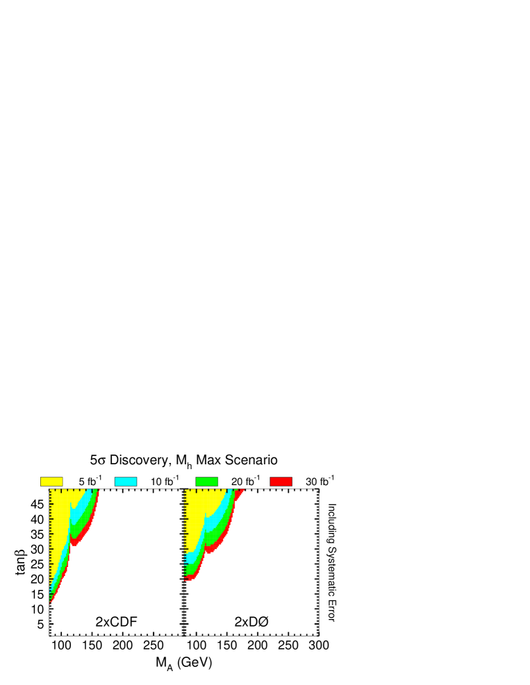
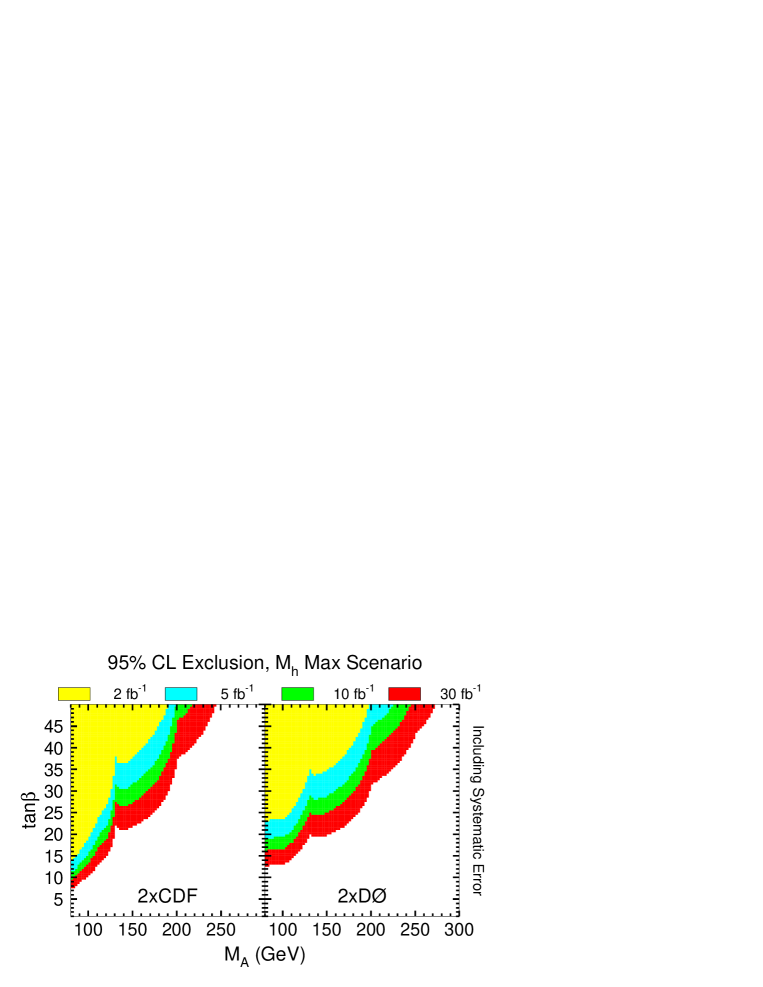
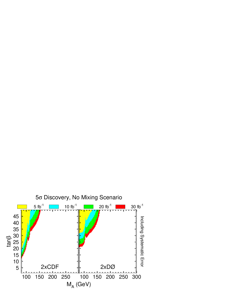
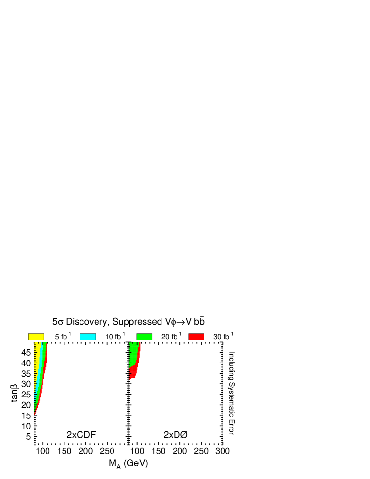
Figs. 115 and 115 are contour plots demonstrating regions of discovery and 95% C.L. exclusion for the maximal mixing benchmark scenario. Clearly, large values of , for which the CP-odd Higgs boson and one of the CP-even Higgs bosons has enhanced couplings to the bottom quarks, are necessary to render the channel experimentally viable. In fig. 117, we show the parameter space coverage for discovery in the no-mixing benchmark scenario. Comparison with fig. 115 shows that the distinction between the maximal squark mixing and no squark mixing cases is small. This can be attributed to the fact that in both cases, the parameter was taken to be rather small; hence, the effects of the vertex corrections to the bottom Yukawa coupling are small. However, this does not mean that the channel is, in general, robust under variation of the MSSM parameters. Precisely at large values of , for which the channel is promising, the vertex corrections to the bottom Yukawa coupling may become quite relevant. As explained in Section I.C., depending on the sign and magnitude of [eq. (30)], large vertex corrections to the bottom Yukawa coupling may be induced varying drastically the coverage of the – plane through the channel. For example, in the suppressed benchmark scenario, since all the Higgs couplings to are generally suppressed, the MSSM parameter coverage is reduced as shown in fig. 117.
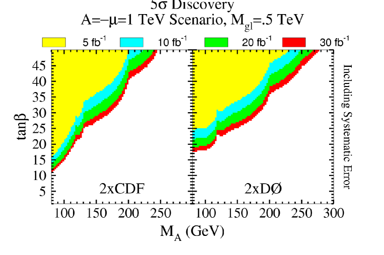
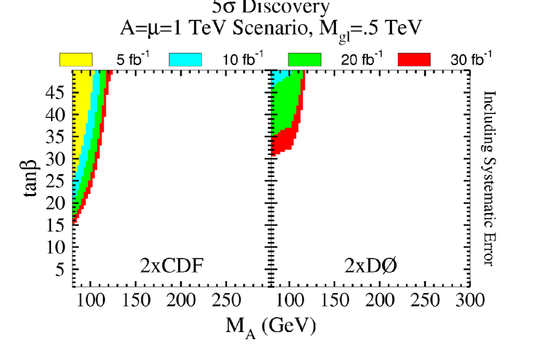
As previously noted, the leading one-loop corrections to the bottom Yukawa coupling suppress [enhance] the coupling for [], thus degrading [improving] the Higgs discovery potential in the channel. In Section I.C.3, the dependence of on the supersymmetric parameters is exhibited [eq. (30)] and its phenomenological implications are discussed. Here, we remind the reader that the sign of is governed by the sign of (in the convention where is positive), as the dominant contribution to from bottom-squark loops is proportional to . The top-squark loop contribution to adds a sub-dominant contribution proportional to , which increases [decreases] the overall magnitude of for []. The dependence of the parameter space coverage on the sign of is illustrated in figs. 119 and 119, which exhibit discovery contours for the case = 1 TeV, = 1 TeV and TeV. These plots illustrate the two possible choices for the sign of , which correspond to different signs for the loop corrections to the Higgs–bottom-quark Yukawa coupling. Moreover, since , the leading one-loop corrections are further enhanced for , thus improving the Higgs discovery potential in the channel. Thus, we see that there can be strong dependence of the potential for discovery on the specific choice of MSSM parameters. Observation of a signal in this channel will clearly suggest that is large, and can place some useful constraints on the allowed regions of MSSM parameter space.
III.2.4 MSSM Higgs Sector Summary
We may combine the results for the various channels obtained in the generic MSSM analysis to provide summary plots of the MSSM Higgs discovery reach of the upgraded Tevatron collider. For comparison, we show in each case the expected LEP final coverage of the – plane obtained from the search mode with the subsequent decay of or into or . Moreover, although not explicitly shown in the final combined plots presented here, the absence of a Higgs signal at LEP2 in the associated production process would rule out the parameter space region defined by GeV and as shown in fig. 11 in the maximal mixing scenario. The reach of the latter channel has not yet been presented in a model independent way by the LEP collaborations. Nevertheless, for the three benchmark scenarios of table 53, the excluded region at low and large will not be appreciably different from the one quoted above.
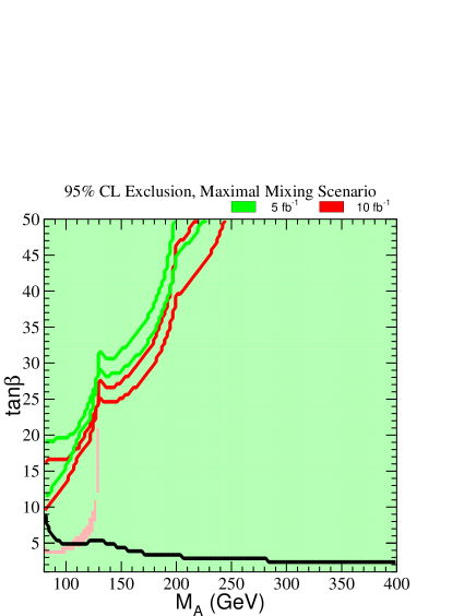
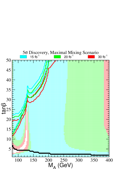
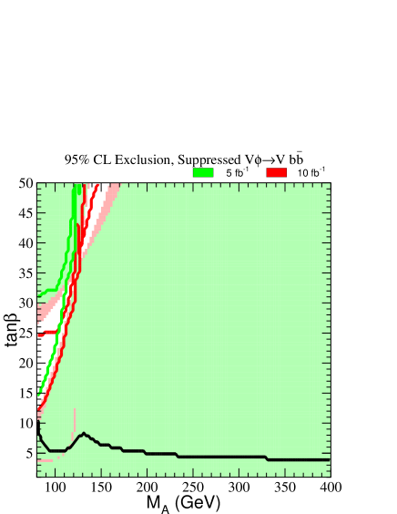
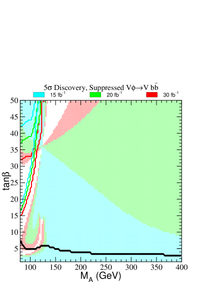
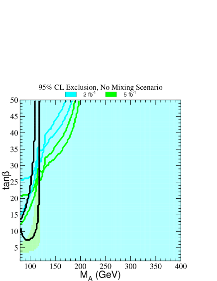
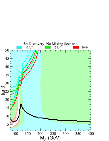
In figs. 120–122, we show the regions of 95 CL Higgs exclusion and Higgs discovery on the – plane, for representative MSSM parameter choices, via the search of neutral Higgs bosons in the channels: [, ], (shaded regions) and , [, , ], (region in the upper left-hand corner bounded by the solid lines), for different integrated luminosities as indicated by the color coding. The two sets of lines (for a given color) bounding the regions accessible by the search correspond to the CDF and DØ simulations, respectively. Finally, the solid black line (usually near the bottom of each plot) reflects the upper limit of (as a function of ) deduced from the absence of observed events at LEP2. The shaded regions presented in these figures reflects the results of the SHW simulation of improved by neutral network techniques, as described in the generic MSSM analysis presented in Section III.B.2. We do not display here the effects of systematic error due to uncertainties in -tagging efficiency, background, mass resolution and other effects. The implications of a 30% reduction in detection efficiency has already been illustrated by comparing lighter and darker color shading in figs. 108–110.
From our results, it follows that in the most demanding scenarios, (shown in figs. 120 and 122), 5 fb-1 of integrated luminosity per experiment will allow one to test nearly all of the MSSM Higgs parameter space at 95% CL. Note the importance of the complementarity between the and channels for improving the coverage of the MSSM parameter space in the low region in fig. 122, where there is a strong reduction of for the CP-even Higgs boson with strongest coupling to the vector gauge bosons.
To assure discovery of a CP-even Higgs boson at the 5 level, the luminosity requirement becomes very important. Figs. 120(b), 122(b) and 122(b) show that a total integrated luminosity of about 20 fb-1 per experiment is necessary in order to assure a significant, although not exhaustive, coverage of the MSSM parameter space. In general, we observe that the complementarity between the two channels, and , is less effective in assuring discovery of a Higgs boson as compared with a 95% CL Higgs exclusion. This is due to the much higher requirement of total integrated luminosity combined with the existence of MSSM parameter regimes which can independently suppress both Higgs production channels. Fig. 122 exhibits one of the most difficult regions of MSSM parameter space for Higgs searches at the Tevatron collider. Nevertheless, even in this case, a very high luminosity experiment can cover a significant fraction of the available MSSM parameter space.
In conclusion, Run 2 of the Tevatron (with an integrated luminosity of 2 fb-1) cannot significantly improve the MSSM Higgs mass limits obtained at LEP. However, if the integrated luminosity can be increased to 10 fb-1 and beyond, then substantial improvements beyond the LEP reach are achievable. Although the upgraded Tevatron cannot probe the entire MSSM Higgs parameter space, integrated luminosities of 20–30 fb-1 would provide close to complete coverage for a 5 discovery of the Higgs boson.
III.3 New Higgs Physics Beyond the Standard Model/MSSM
M.C. Gonzalez-Garcia, S.M. Lietti and S.F. Novaes
Effective Lagrangians provide a formalism for a model-independent description of new TeV-scale physics beyond the Standard Model. An effective Lagrangian for gauge boson–Higgs boson interactions was presented in eqs. (43)–(I.4). A set of new effective Higgs couplings are thus introduced that in principle can be measured in future experiments. In the Standard Model, these effective couplings are generated at the loop level. Thus, to discover physics beyond the Standard Model, one would have to measure these couplings with sufficient accuracy to detect deviations from Standard Model predictions.
In this section, we discuss the present limits on anomalous Higgs couplings and evaluate the improved limits attainable from searches at the upgraded Tevatron. Since the Higgs boson in the model-independent approach is not strictly the Standard Model Higgs boson (although the deviation from Standard Model behavior may be small), we shall henceforth denote the Higgs boson by for the remainder of this section.
Present Bounds from Searches at Tevatron Run 1 and LEP2
Anomalous Higgs boson couplings have been studied in Higgs and boson decays in ee ; our:lep2aaa ; our:NLCWWA ; our:NLCZZA and in collisions our:tevatronjj ; our:tevatronmis ; our:tevatron3a ; our:combined . The combined bounds on anomalous Higgs boson interactions are derived from the following data:
| (86) |
Events containing two photons plus missing transverse energy (), additional photons or charged fermions represent a signature for several theories involving physics beyond the SM. In the framework of anomalous Higgs couplings presented in eqs. (43)–(I.4), they can arise from the production of a Higgs boson which subsequently decays in two photons [second column in Eq.(LABEL:proc)]. Recent analyses of these signatures showed a good agreement with the expectations from the SM. Thus, these negative experimental results can be used to constrain new anomalous couplings in the bosonic sector of the SM.
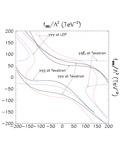

DØ has searched for high invariant–mass photon pairs in events d0jj at TeV and pb-1 of integrated luminosity. No events were observed with two–photon invariant mass in the range , which constrains the anomalous Higgs boson couplings defined in eq. (I.4) that lead to the process our:tevatronjj . In the analysis of ref. concha , the cuts of ref. d0jj were applied and included the particle identification and trigger efficiencies. The searches discussed here are limited to a Higgs boson with mass in the range , since after the threshold is reached the diphoton branching ratio of Higgs is quite reduced.
DØ has also searched for events with two photons and large missing transverse energy d0miss . No events were observed in the invariant mass range . This can be used to constrain operators leading to the processes and , where the lepton is not detected our:tevatronmis . To compare with the DØ results d0miss , the same cuts as in the last article in ref. d0miss were applied, including the particle identification and trigger efficiencies which vary from 40% to 70% per photon. After these cuts, 80% to 90% of the signal comes from associated production while 10% to 20% arises from production.
CDF has searched for events with three photons, requiring two photons in the central region of the detector, with a minimum transverse energy of 12 GeV, plus an additional photon with GeV, and a photon separation of at least cdf . These results have been used to constrain operators leading to . These same operators can be constrained by results for electron–positron collisions our:lep2aaa , in particular the recent OPAL results opal:ggg , where data taken at several energy points in the range – GeV were combined.
The calculations have included all SM (QCD plus electroweak), and anomalous contributions that lead to these final states. The SM one-loop contributions to the and vertices were introduced through the use of the effective operators with the corresponding form factors in the coupling. Neither the narrow–width approximation for the Higgs boson contributions, nor the effective boson approximation were employed. The interference effect between the anomalous signature and the SM background have been included consistently. For all analyses, the MRS (G) mrs set of proton structure functions were employed with the scale .
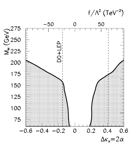
The coupling [see eq. (44)] involves and hagiwara2 . As a consequence, the anomalous signature is only possible when those couplings are not vanishing. The couplings and , on the other hand, affect the production mechanisms for the Higgs boson. Fig. 123 (a) shows the excluded region in the , plane from the different channels studied for GeV, assuming that these are the only non–vanishing couplings. Since the anomalous contribution to is zero for (see eq. (44)), the bounds become very weak close to this line, as is clearly shown in fig. 123. Note that these bounds are based on Poisson statistics.
The results obtained from the analysis of the four reactions (eq. (LABEL:proc)) can be statistically combined in order to constrain the value of the coefficients , of (eq. (43)) our:combined . Fig. 123 (b) exhibits the 95% CL exclusion region in the plane obtained from combined results.
In order to reduce the number of free parameters, one can make the assumption that all blind operators affecting the Higgs interactions have a common coupling . Fig. 124 shows the combined limits for the coupling constant for Higgs boson masses in the range of GeV.
Attainable Bounds at the Upgraded Tevatron
The effect of the anomalous operators becomes more evident with the increase of energy, and therefore, higher sensitive to smaller values of the anomalous coefficients can be achieved by studying their contribution to different processes at the upgraded Tevatron collider. Estimates for the upgraded Tevatron, with 1 fb-1 and 10 fb-1 respectively are considered here. For the reactions and , Run 1 cuts and efficiencies are used. For the final state, the effects of additional kinematic cuts to improve the sensitivity have been considered our:tevatron3a . The best results in this case are obtained for the following set of cuts: GeV, with GeV, where the three photons are ordered according to their transverse energy, i.e. , and . For these estimates, the CDF Run 1 detection cdf efficiency for photons has been assumed.
| (TeV-2) | ||||
|---|---|---|---|---|
| (GeV) | Combined | |||
| 100 | (24, 24) [13, 15] | (16, 36) [9.4, 26] | (9.2, 22) [3.3, 5.6] | (7.6, 19) [3.0, 5.6] |
| 120 | (26, 26) [14, 14] | (20, 39) [15, 27] | (8.6, 21) [3.4, 5.9] | (7.4, 18) [3.3, 5.9] |
| 140 | (30, 31) [15, 16] | (25, 44) [14, 30] | (10, 23) [4.5, 8.9] | (9.1, 20) [4.0, 8.7] |
| 160 | (36, 38) [17, 19] | (29, 50) [14, 33] | (11, 24) [6.0, 14] | (9.9,22) [5.1, 13] |
| 180 | (—, —) [—, —] | (63, 72) [46, 53] | (26, 34) [16, 24] | (24, 33) [16, 24] |
| 200 | (—, —) [—, —] | (87, 90) [50, 53] | (33, 40) [17, 23] | (32, 39) [17, 23] |
| 220 | (—, —) [—, —] | (—, —) [—, —] | (42, 45) [19, 26] | (42, 45) [19, 26] |
Table 54 contains the 95% CL limit on the anomalous couplings for the upgraded Tevatron for each individual process. All couplings are assumed equal () and the Higgs boson mass is varied in the range GeV. Combination of the results obtained from the analysis of the first three reactions in eq. (LABEL:proc) leads to the improved bounds given in the last column of Table 54. Comparing these results with those in fig. 124, we observe an improvement of about a factor 2–3 [ 4–6] for the combined limits at the upgraded Tevatron with 1 fb-1 [10 fb-1] integrated luminosity.
As mentioned previously for linearly realized effective Lagrangians, the modifications introduced in the Higgs boson and in the vector boson sectors are related to each other. Consequently, the bounds on the new Higgs couplings should also restrict the anomalous gauge–boson self interactions. Under the assumption of equal coefficients for all anomalous Higgs operators, the common Higgs boson anomalous coupling can be related to the conventional parameterization of the vertex (, ) hhpz ,
| (87) |
A different set of parameters has been also used by the LEP Collaborations in terms of three independent couplings, , , and , These parameters are related to the parameterization of Ref. hhpz through , , . Under the relations given in eq. (87) they verify .
The current experimental limit on these couplings from combined results on double gauge boson production at Tevatron and LEP2 vancouver is at 95 % CL. This limit is derived under the relations given in eq. (87) hisz and it is plotted in fig. 124 for comparison with the bounds obtained from this analysis.
Table 55 contains the 95% CL limit on the anomalous coupling using the limits on obtained through the analysis of the processes in eq. (LABEL:proc). The expected bounds that are attainable at the upgraded Tevatron are also shown. These results show that the present combined limit from the Higgs production analysis obtained here is comparable with the existing bound from gauge boson production for GeV.
| Process | |
|---|---|
| Combined Tevatron Run 1 + LEP2 | (0.084, 0.204) |
| Combined Tevatron Run 2 (1 fb-1) | (0.048, 0.122) |
| Combined Tevatron Run 2 (10 fb-1) | (0.020, 0.036) |
IV Summary and Conclusions
The next run of the Tevatron proton-antiproton collider at Fermilab will see enormous increases in luminosity, initially more than an order of magnitude larger than those in Run 1. With the new Main Injector and Antiproton Recycler rings a total integrated luminosity of 2 fb-1 should be delivered to the CDF and DØ collider experiments by the end of 2002. Continuous running over multiple years and additional improvements to the collider could result in a total data sample exceeding 10 fb-1 prior to the start of the LHC. Both CDF and DØ will have greatly improved detectors, with all new charged particle tracking and vertexing, improved calorimetry and triggering, and new offline analysis software. These improvements to the accelerator and the detectors enhance the sensitivity of the experiments for new particle searches. In particular, given sufficient integrated luminosity, the discovery of the Higgs boson at the upgraded Tevatron collider may be within reach.
In Run 1, the CDF and DØ collaborations began developing the techniques for searching for the Higgs bosons of the Standard Model (SM) and Minimal Supersymmetric Standard Model (MSSM). The Tevatron Run 1 integrated luminosity of about 100 pb-1 was too small to yield sufficient sensitivity to exclude or discover the SM Higgs. In the MSSM, certain Higgs fermion-couplings are enhanced (relative to their Standard Model values) in some regions of MSSM parameter space. As a result, one can already deduce some weak restrictions on the MSSM Higgs parameters based on the Run 1 MSSM Higgs searches for neutral Higgs production (in association with pairs) and charged Higgs bosons (resulting from top decays). This Report capitalizes on the experience gained in Run 1 in estimating the discovery and exclusion reach for the SM and MSSM Higgs bosons in Run 2, assuming that CDF and DØ combine their results to maximize the sensitivity.
Estimating the discovery and exclusion reach for Higgs bosons requires accurate knowledge of the search acceptance and expected backgrounds in the various channels. No detailed simulation existed prior to this Workshop, and so the participants developed SHW—a simple Monte Carlo simulation—to represent an “average” of the CDF and DØ experiments, taking into account the improvements to the detectors. SHW simulates the detector response to all the individual particles in the event, including tracking and calorimeter efficiency, resolution, and geometry, but does not simulate the effects of multiple interactions, the magnetic field, lateral shower development, secondary interactions, or details of the microvertex detectors. Comparisons of the simulation with the Run 1 full simulation and data are encouraging, and show agreement at the 15-20% level in acceptance.
Without the real Run 2 data, it is also difficult to get an accurate estimate of the quark jet tagging efficiency and mistag rate, the jet-jet mass resolution, and certain backgrounds that must be estimated from actual data. The philosophy in this study is to make an optimistic yet realistic estimate of the Higgs boson discovery and exclusion reach, assuming improvements to these performance parameters of the detectors and analyses. These estimates are based on Run 1 experience, albeit with less capable detectors, and detailed simulations of -tagging at the planned Run 2 detectors. Further work will be necessary to understand some of the relevant backgrounds with higher level of accuracy. The completion of the background analyses will also require direct handling of the actual Run 2 data. A more accurate estimate of the Run 2 Higgs discovery and exclusion reach can only be achieved after the Tevatron Run 2 experiments start collecting data.
Search for the Standard Model Higgs Boson \\
In the mass region of interest to the Tevatron (100 GeV GeV), the SM Higgs boson is produced most copiously via fusion, with a cross section from about 1–0.1 pb. For GeV, the Higgs boson decays dominantly to . Since the cross section for the QCD production of dijet events is orders of magnitude larger than the Higgs production cross section, the channel is not a promising channel and thus has not been investigated in this Report. For GeV, the Higgs boson decays dominantly to (where is a virtual ), and the channel is accessible to the Tevatron Higgs search.
The next largest Higgs cross section is for the production of the SM Higgs boson in association with a vector boson. The combined and cross sections is about 0.2—0.5 pb in the mass region of interest ( GeV), while the dominant Higgs decay is . These processes lead to four main final states: , , , and . Of these channels the first three have distinct signatures on which the experiments can trigger (high leptons and/or missing ) and the backgrounds are controllable, typically dominated by vector-boson pair production, production and QCD dijet production. The backgrounds can in all cases be estimated and/or cross-checked with actual data, allowing the systematic error to remain roughly a constant fraction of the total background. The signal efficiencies and backgrounds have all been estimated with both the CDF Run 1 detector simulation and with the simple SHW simulation. In addition, the selection was optimized using neural network techniques, resulting in a demonstrable gain in the significance of the Higgs signal for the and channels.
As noted above, the -tagging efficiencies and the mass resolution play a key role in determining the ultimate efficiency and background rejection. Much work remains, using real data studies, to optimize the performance in both these areas. In this regard, we have been optimistic in this Report, assuming a “loose” -tag efficiency of 75% at large jet , and a “tight” -tag efficiency of 60% at large jet . We believe that these are realistic numbers, based on simulation studies. For the mass resolution, we have assumed in the final results a 10% resolution on the “core” of the distribution; inefficiencies due to the low side tail remain after this rescaling of the simulation output. This is aggressive, but simulations suggest that a 10% mass resolution may be achievable. Moreover, given CDF’s demonstrated 12% mass resolution in events at Run 1, we believe that an ultimate goal of a 10% mass resolution is not overly optimistic.
For backgrounds we have used Monte Carlo estimates everywhere except in the channel, where there is a significant contribution from QCD dijet production. This background comes from the extreme tail of a very large cross section, and is thus very difficult to model. In the CDF Run 1 analysis of this channel, QCD dijets constituted half of the total background. DØ searches involving the same topologies have considerably lower background levels, despite the absence of a tag requirement, due to their better missing resolution. To be conservative, we have taken the unknown QCD dijet background to the channel to be equal in size to the sum of all other contributing background processes.
Larger Higgs masses ( GeV) had not been studied in previous Tevatron studies. This Workshop produced several analyses aimed at exploiting the distinct signatures present when the Higgs boson decay branching ratio to becomes appreciable. In this case, there are final states with (from the gluon-fusion production of a single Higgs boson), and and arising from associated vector boson–Higgs boson production. Three search channels emerged in the Workshop as potentially sensitive at these high Higgs masses: like-sign dilepton plus jets () events, high- lepton pairs plus missing (), and trilepton () events. Of these, the first two were found to be most sensitive.
Note that in this study, the same analysis selection has been assumed for integrated luminosities ranging over an order of magnitude. This is not the typical pattern in new particle searches in high energy physics: as the integrated luminosity increases, better understanding of signal and background separation typically leads to the tightening of selection cuts in order to keep background low while maintaining the signal efficiency. Of course, some backgrounds will remain irreducible, but it is possible that the integrated luminosity thresholds could be lowered with respect to those reported here, as experience is gained with real data.
The final combined result of the integrated luminosity required to exclude or discover the SM Higgs boson, as a function of the Higgs mass, depicted in fig. 103, is obtained by combining the sensitivity of all the channels described above, and assuming that the data from the CDF and DØ experiments can be combined. This result is achieved by forming a joint likelihood from the product of the Poisson probabilities of single-channel counting of signal and background in each channel. A nominal systematic error on the expected background was taken into account by Bayesian integration.
The final result shows that for an integrated luminosity of 10 fb-1, if the SM Higgs boson does not exist in the energy range explorable at the Tevatron, then one can attain a 95% CL exclusion for masses up to about 180 GeV. Moreover, if the SM Higgs happens to be sufficiently light ( GeV), then a tantalizing effect will be visible with the same integrated luminosity. With about 25 fb-1 of data, evidence for the Higgs boson can be obtained for the entire Higgs mass range up to 180 GeV. However, the discovery reach is considerably more limited for a 5 Higgs boson signal. Even with 30 fb-1 of integrated luminosity, only Higgs bosons with masses up to about 130 GeV can be detected with 5 significance.
Suppose that the Higgs boson mass is 115 GeV, which lies just above the 95% CL exclusion limit achieved by LEP tomjunk . At the Tevatron, with 5 fb-1 of integrated luminosity per experiment, there would be sufficient data to see a 3 excess above background, providing evidence for a Higgs boson. With 15 fb-1 of integrated luminosity per experiment, a discovery of the Higgs boson would be possible.
The above integrated luminosity requirement crucially depend on the success of a greatly improved mass resolution and -tagging rates (as compared to Run 1). Nevertheless, these results clearly provide strong motivation to the accelerator division to deliver the largest possible integrated luminosity, and to the experimental collaborations to optimize the data analyses and reconstruction techniques, and continue to study new methods and ideas for enhancing the sensitivity in this search.
Other Higgs signatures could help improve the sensitivity of the Higgs search at the Tevatron. In this Report, none of the channels corresponding to the decay mode of the Higgs have been investigated, as the small branching ratio (less than ) makes the corresponding signal rates small. Still, a significant improvement of -lepton identification could lead to a viable Higgs signal in the low Higgs-mass ( GeV) regime. This possibility deserves further study. Perhaps more promising is the detection of the Higgs boson via production (the Higgs boson is radiated off the top-quark), followed by . Initial studies rainwater suggest that this channel could be observable at the upgraded Tevatron, with a statistical significance comparable to the Higgs signals in the and channels. Clearly, if this is confirmed by a more detailed analysis, it would improve the prospects for a Higgs signal at the Tevatron, perhaps even lowering significantly the total integrated luminosity required for evidence of a Higgs signal or a discovery.
Search for Higgs Bosons of Low-Energy Supersymmetry \\
The possibility that nature is supersymmetric at the TeV scale opens up several new experimental alternatives in the search for Higgs bosons. The Minimal Supersymmetric Standard Model (MSSM) requires two Higgs doublets, which yields five physical scalars: two CP-even neutral scalars ( and ), a CP-odd scalar () and a charged Higgs pair (). At tree level, the masses and couplings of these particles are governed by two parameters, (the ratio of the two neutral Higgs field vacuum expectation values) and one of the Higgs masses (usually chosen to be ). When loop effects are taken into account, one finds that Higgs masses and couplings depend additionally on various supersymmetric mass parameters. Such effects can be significant in certain regions of the MSSM parameter space. These include an increase in the upper bound of the mass of the lightest CP-even Higgs boson ( GeV, assuming an average top squark mass no larger than 1 TeV), a possible suppression or enhancement of the dominant decay rate (where , , and/or ), and CP-violating effects that can mix the CP-even and CP-odd eigenstates.
In various regimes of the — parameter space, the phenomenology of the Higgs bosons can be very different. For example, in the regime where , known as the decoupling limit, the light scalar possesses the same production cross-sections and decay rates as , and is thus indistinguishable from the SM Higgs boson. In this case, the SM Higgs search analyses apply, while all other Higgs bosons are too heavy and not observable at the Tevatron. In contrast, if , then the properties differ significantly from those of . In this parameter range, it may be possible to detect more than one Higgs state at the Tevatron, or demonstrate that an observed Higgs signal does not correspond to the one expected from the SM Higgs boson.
In the latter case, we can still make use of the Standard Model Higgs analyses as follows. For each Higgs production/decay channel, we first define theoretical ratios (denoted collectively by ) of for Higgs production and decay in the MSSM relative to its Standard Model value. Then, we can derive a lower limit for the required luminosity in order to obtain a Higgs signal of fixed significance (e.g. 95% CL limit or a discovery). If , the result for is simply the one obtained in the Standard Model Higgs search analysis. If , then we expect to be constant in the Gaussian limit, which yields a lower limit for as a function of (say, at fixed Higgs mass). In the regime where Poisson statistics is required, this scaling is somewhat modified; the corresponding -plots were given in Section III.B.1.
The MSSM analysis proceeds as follows. The Higgs signatures arising from associated vector boson–Higgs boson production followed by Higgs decay to , treated in the SM analysis, also apply to the case of the CP-even Higgs bosons of the MSSM. For a given point in supersymmetric parameter space (which depends on , , and other supersymmetric mass parameters, such as the third generation squark masses, the gaugino masses, the trilinear couplings , and higgsino mass parameter , which govern the size of the radiative corrections), one can compute the corresponding values for the associated vector boson–Higgs boson production and subsequence Higgs decay to . Comparing with the -plots previously obtained, one can then either exclude or discover a CP-even Higgs boson of a given mass for a fixed integrated luminosity. In this way, one can map out the MSSM Higgs parameter space in the — plane (under various assumptions for the values of the other supersymmetric parameters that govern the impact of the loop-effects) and determine which parameter regimes are accessible to the Tevatron Higgs search at a given luminosity.
We have studied three examples: (i) the top-squark (stop) mixing parameters is set to zero, which minimizes the maximal value of the radiatively-corrected light CP-even Higgs mass (the so-called “minimal-mixing” or “no-mixing” scenario); (ii) the stop mixing parameters are chosen to maximize the value of the lightest CP-even Higgs mass (the “maximal-mixing” scenario); and (iii) the stop mixing parameters and the gluino mass are chosen in order to suppress the coupling of the Higgs state that is primarily produced in association with the gauge bosons (the “suppressed production” scenario). Case (iii) exemplifies a possible worst case scenario for the MSSM Higgs search at the upgraded Tevatron. In the case of minimal mixing, a Higgs boson produced in association with the gauge bosons may be excluded at the 95 CL with as little as 5 fb-1 of data per experiment, and can be discovered at the level over nearly the entire region of the — plane with less than 20 fb-1 per experiment. However, in the other two cases mentioned above, our results show that an integrated luminosity of order 20—30 fb-1 is required to obtain a 5 discovery over a significant portion of the parameter space. Yet, even in these cases, 10 fb-1 is sufficient to exclude the Higgs sector of the MSSM at the 95 CL, for most values of and (independent of the values of the stop mixing parameters, assuming that the average top squark mass is not much larger than 1 TeV), if no Higgs signal is detected. However, in the suppressed production scenario, there is a non-negligible region of the MSSM parameter space in which even a 95 CL Higgs exclusion limit is not achievable at 30 fb-1. Note that if the Higgs signature due to (with ), examined in ref. rainwater , proves to be a viable discovery mode, then the analogous MSSM Higgs signatures could improve the upgraded Tevatron coverage of the MSSM Higgs parameter space described above.
In the large regime of the MSSM, some of the neutral Higgs boson couplings to down-type fermions (such as ) are enhanced, and lead to production cross sections for Higgs bosons that are significantly larger than those of the Standard Model Higgs boson. As a result, in general two of the neutral Higgs bosons of the MSSM can also be discovered in an additional channel: production, followed by (where is either the CP-odd Higgs boson or the neutral CP-even Higgs boson with enhanced coupling to , at large ). The corresponding channel cannot be observed in the case of the SM Higgs boson, since the coupling is suppressed by a factor of and has no additional enhancement. The production of a neutral MSSM Higgs boson in association with a pair followed by Higgs decay to leads to a distinctive final state with four high- jets. These events can be observed by positively tagging at least three of these -jets, which dramatically reduces the QCD multijet background. The cross section for this process is proportional to , and is thus greatly enhanced at large . The studies presented in this Workshop show that an interesting region of the MSSM parameter space at high is accessible in Run 2. In particular, some limits already emerge with 2 fb-1 of data in the region of high and low . The region of sensitivity grows to slightly lower values of and larger values of as the luminosity is increased further. However, one finds that there are large supersymmetric and QCD corrections that must be taken into account, which will require detailed theoretical analysis in the coming years. Nevertheless, the enhanced production process increases the overall sensitivity of the Tevatron MSSM Higgs search, and provides some complementary coverage in the — plane with respect to the associated vector boson–Higgs boson production discussed above.
Finally, if the charged Higgs boson is light enough so that the decay is allowed, then the Tevatron Higgs boson search at Run 2 can discover the charged Higgs boson if is sufficiently larger than 1 (or smaller than 1, although the latter is disfavored by theoretical considerations). Again, it is possible to see a signal at Run 2 at large values of and small values of (the latter is required in order that ). With additional luminosity, the region of sensitivity in also grows, although the ultimate region of MSSM parameter space at accessible by the charged Higgs search is not as great as the corresponding region accessible by the search for enhanced production.
Conclusions \\
The search for the Higgs boson and the dynamics responsible for electroweak symmetry breaking is the central goal of high energy physics today. The Tevatron experiments, if given sufficient data, are poised to make major advances in meeting this goal. A great deal of effort remains in order to raise the performance of the accelerator to the level demanded by the Higgs search. The nominal yearly integrated luminosity for Run 2 is 2 fb-1 per year. However, 10—30 fb-1 of data (per experiment) is needed to significantly improve the Higgs search beyond the current LEP2 limits, with the higher luminosity crucial for maximizing the coverage both in the Standard Model and its supersymmetric extension.
Further challenges must be met in bringing the detectors on line and fully operational, and in developing the techniques and understanding, particularly in jet-jet mass reconstruction and jet tagging, necessary to extract the faint signal of the Higgs boson from the larger Standard Model background. In some cases, we were perhaps optimistic with regard to the expected capabilities of the detector. However, this Report clearly points to some important goals that the experimental detectors and analysis methods must achieve if the Higgs search at the Tevatron is to be successful. In some cases, the magnitude of the Standard Model backgrounds are not known at the required level of accuracy. Additional theoretical work along with background studies once higher luminosity data become available will be crucial for improving the Higgs search strategies and maximizing the chances for uncovering the Higgs signal. We believe that the results obtained in this Report provide a useful attempt to devise a realistic search strategy for Higgs bosons, and provide a benchmark for future improvements.
The LHC is expected to begin its physics run in 2006. The search for the Higgs boson is one of the primary missions of the ATLAS and CMS detector collaborations. With much larger annual luminosities and energies, they will discover the Higgs boson (in most theoretical scenarios) if it has not yet been observed. There is a window of opportunity for the Tevatron that will be open for the next six to seven years. With a little luck and a great deal of determination, the Higgs boson can be discovered at a sufficiently upgraded Tevatron. The potential physics payoff is great, and provides a strong motivation to do the work necessary to meet this challenge in the pre-LHC era.
APPENDIX
Appendix A Statistical Method for Combining Channels
John Conway, Howard Haber, John Hobbs, Harrison Prosper
The statistical method employed here for combining channels follows an essentially Bayesian approach by forming a joint likelihood for a given set of experimental outcomes, as a function of a dummy multiplier on the theoretical cross section.
For each search channel assume that we expect events from the Higgs signal and events from all backgrounds, in 1 fb-1 integrated luminosity. These values, then, can equivalently be thought of as the accepted signal and background cross sections in units of femtobarns.
In the actual experiments, after some integrated luminosity L has been recorded, one expects L signal and L background in a given channel , and observes some number . The Poisson probability for observing events, where events are expected in this channel is well known:
The joint likelihood for all channels is simply the product of these probabilities:
This likelihood tells us the absolute probability of our particular experimental outcome, but gives no information about whether or not a signal is actually present. To accomplish this one can introduce a factor which multiplies the expected signal, and determine confidence intervals on its true value from a probability density function (p.d.f.) based on the joint likelihood above. Thus, we now have , and from Bayes’ Theorem we find that this “posterior” p.d.f. can be written as
where we have expressed the sets , , and as vectors for clarity. If there is no Higgs then the function will be maximum at , and fall more and more sharply as the integrated luminosity increases. If, on the other hand, there is a Higgs (at the mass were are considering), then the posterior p.d.f. will be more and more sharply peaked at as L increases.
For a given integrated luminosity L and a given experimental outcome, then, how can one use the posterior p.d.f. in to either claim a discovery at some level of significance or exclude the predicted Higgs cross section with come confidence?
For discoveries, one usually quotes significance in units of , (say, or ) where it is understood that this refers to equivalent Gaussian standard deviations. In the method used here one finds that value of at which is a maximum, , and compares with the value evaluated for . That is, one compares the maximum likelihood to that of the null hypothesis. One can then find the number of “equivalent Gaussian ” from the ratio of these values:
and so the significance can be written as
For exclusion limits, or confidence intervals on in general, one simply performs integrals of the posterior p.d.f., which by definition is normalized to unity. Thus if we desire a 95% confidence level exclusion, we need to find that value of for which
where . If, for example, there is no Higgs and we find that we can exclude at 95% CL any value of , then we conclude that the Higgs is excluded at that confidence level, since corresponds to the Standard Model prediction for the Higgs cross section.
One can also take into account systematic errors using this method, by convoluting Gaussians representing the relative uncertainties in the and with the expression for the joint likelihood. In the method used here this is approximated by a coarse numerical integration in the likelihood calculation.
The main goal of the Higgs studies presented here, however, is to estimate the integrated luminosity needed to reach certain thresholds of significance. But clearly for a given set of expected number of signal and background events, at a certain integrate luminosity, there are many possible future experimental outcomes, some of which will and some of which will not meet the desired level of significance. Following the precedent of the LEP-II Working Group, we simply seek that integrated luminosity at which 50% of the possible future outcomes would meet the desired level.
To actually calculate these integrated luminosity thresholds requires simulating a large ensemble of pseudoexperiments, each representing a certain outcome, distributed according to their actual probability of occurrence. Then, one varies the integrated luminosity until the 50% criterion is met. Note that in the case of determining 95% CL limits, the program generates no signal events in each pseudoexperiment, whereas in the case of determining discovery thresholds, the program does generate signal events in each pseudoexperiment.
A few notes about the statistical method are in order. Firstly, in the case of a single channel with no systematic errors, for setting 95% CL limits, the Bayesian method outlined above is in exact agreement with the commonly used frequentist method described in the 1996 PDG Review of Particle Properties. In that approach one excludes at some confidence level any value of greater than that for which
This formula simply asks for that level of expected signal such that the probability of seeing or fewer events, and having or fewer background, is less than some value .
Also, in the limit of high statistics, the results of the Bayesian method outlined above agree closely with those from what one might call the “naive Gaussian approximation.” This approximation uses the values of the and to form “significances” , and then finds those values of L for which exceeds some value, namely 3 or 5 for and discoveries, respectively, and 1.96 for a 95% CL limit. This commonly used approximation breaks down, of course, in the low-statistics regime where the distributions are Poisson and not well approximated by Gaussians.
References
- (1)
- (2) F. Abe et al., [CDF Collaboration], Phys. Rev. Lett. 74 (1995) 2626; S. Abachi et al., [DØ Collaboration], Phys. Rev. Lett. 74 (1995) 2632.
- (3) D. Abbaneo et al [ALEPH, DELPHI, L3 and OPAL Collaborations, LEP Electroweak Working Group, and SLD Heavy Flavour and Electroweak Groups], CERN-EP-2000-016.
- (4) A. Straessner, talk given at the XXXVth Rencontres de Moriond (March, 2000).
- (5) D. Strom, talk given at the 5th International Symposium on Radiative Corrections (RADCOR-2000), Carmel, CA, 11–15 September, 2000.
- (6) E. Farhi and L. Susskind, Phys. Rep. 74 (1981) 277; R. K. Kaul, Rev. Mod. Phys. 55 (1983) 449; K. Lane, in The Building Blocks of Creation—From Microfermis to Megaparsecs, Proceedings of the Theoretical Advanced Study Institute (TASI 93) in Elementary Particle Physics, Boulder, CO, 6 June—2 July 1993, edited by S. Raby and T. Walker (World Scientific, Singapore, 1994).
- (7) For a review, see I. Antoniadis and K. Benakli, Int. J. Mod. Phys. A15 (2000) 4237.
- (8) A.G. Cohen, in The Building Blocks of Creation—From Microfermis to Megaparsecs, Proceedings of the Theoretical Advanced Study Institute (TASI 93) in Elementary Particle Physics, Boulder, CO, 6 June—2 July 1993, edited by S. Raby and T. Walker (World Scientific, Singapore, 1994).
- (9) P. Bock et al. [ALEPH, DELPHI, L3 and OPAL Collaborations, The LEP working group for Higgs boson searches], CERN-EP-2000-055.
- (10) S. Andringa et al., [ALEPH, DELPHI, L3 and OPAL Collaborations, The LEP working group for Higgs boson searches], paper submitted to ICHEP 2000, Osaka, Japan, 27 July–2 August 2000.
- (11) T. Junk, “Searches at LEP”, presented at the 5th International Symposium on Radiative Corrections (RADCOR-2000), Carmel, CA, 11–15 September, 2000; “Combined LEP Higgs Searches”, presented at the LEP Fest, 10 October 2000.
- (12) The most recent analysis of this type can be found in: T. Hambye and K. Riesselmann, Phys. Rev. D55 (1997) 7255.
- (13) The most recent analyses of this type can be found in: G. Altarelli and G. Isidori, Phys. Lett. B337 (1994) 141; J.A. Casas, J.R. Espinosa and M. Quirós, Phys. Lett. B342 (1995) 171; B382 (1996) 374.
- (14) K. Riesselmann, DESY-97-222 (1997) [hep-ph/9711456].
- (15) J.F. Gunion, H.E. Haber, G. Kane and S. Dawson, The Higgs Hunter’s Guide (Perseus Publishing, Reading, MA, 2000).
- (16) E. Gross, A.L. Read and D. Lellouch, CERN-EP/98-094 (1998), in Results and Perspectives in Particle Physics, Proceedings of the 12th Rencontres de Physique de la Vallee d’Aoste, La Thuile, Italy, 1–7 March, 1998, edited by Mario Greco, Istituto Naz. Fis. Nucl., 1998 (Frascati Physics Series, Volume 12).
- (17) M. Spira, hep-ph/9810289.
- (18) A. Djouadi, J. Kalinowski and M. Spira, Comput. Phys. Commun. 108 (1998) 56. The HDECAY program is available to the public from http://home.cern.ch/ mspira/proglist.html.
- (19) A. Djouadi, M. Spira and P.M. Zerwas, Z. Phys. C70 (1996) 427.
- (20) H. Fusaoka and Y. Koide, Phys. Rev. D57 (1998) 3986.
- (21) A. Djouadi, J. Kalinowski and P.M. Zerwas, Z. Phys. C70 (1996) 435; S. Moretti and W.J. Stirling, Phys. Lett. B347 (1995) 291 [E: B366 (1996) 451].
- (22) T.G. Rizzo, Phys. Rev. D22 (1980) 389; W.-Y. Keung and W.J. Marciano, Phys. Rev. D30 (1984) 248; R.N. Cahn, Rep. Prog. Phys. 52 (1989) 389.
- (23) See e.g., ATLAS Collaboration, ATLAS Detector and Physics Performance: Technical Design Report, Volume 2, ATLAS TDR 15, CERN/LHCC 99-15. The LHC Higgs search is discussed in Chapter 19.
- (24) A complete computer program library with cross-sections for all Higgs production processes relevant to the Tevatron Higgs search is available from http://home.cern.ch/ mspira/proglist.html.
- (25) D. Dicus, T. Stelzer, Z. Sullivan and S. Willenbrock, Phys. Rev. D59 (1999) 094016.
- (26) M. Spira, private communication. Spira has computed the QCD NLO correction to and has confirmed the results first obtained in ref. DSSW .
- (27) A. Stange, W. Marciano and S. Willenbrock, Phys. Rev. D49 (1994) 1354; D50 (1994) 4491.
- (28) T. Han and S. Willenbrock, Phys. Lett. B273 (1991) 167.
- (29) S. Mrenna and C. P. Yuan, Phys. Lett. B416 (1998) 200.
- (30) M. Spira, Fortschr. Phys. 46 (1998) 203.
- (31) R.K. Ellis and S. Veseli, Phys. Rev. D60 (1999) 011501.
- (32) H. Georgi, S. Glashow, M. Machacek and D.V. Nanopoulos, Phys. Rev. Lett. 40 (1978) 692.
- (33) A. Djouadi, M. Spira and P.M. Zerwas, Phys. Lett. B264 (1991) 440; S. Dawson, Nucl. Phys. B359 (1991) 283.
- (34) D. Graudenz, M. Spira and P.M. Zerwas, Phys. Rev. Lett. 70 (1993) 1372; M. Spira, A. Djouadi, D. Graudenz and P.M. Zerwas, Nucl. Phys. B453 (1995) 17.
- (35) M. Krämer, E. Laenen and M. Spira, Nucl. Phys. B511 (1998) 523.
- (36) C. Balázs and C.-P. Yuan, Phys. Lett. B478 (2000) 192.
- (37) C.R. Schmidt, Phys. Lett. B413 (1997) 391; D. de Florian, M. Grazzini and Z. Kunszt, Phys. Rev. Lett. 82 (1999) 5209.
- (38) C. Nelson, Phys. Rev. D37 (1988) 1220.
- (39) M. Dittmar and H. Dreiner, Phys. Rev. D55 (1997) 167.
- (40) T. Han, G. Valencia and S. Willenbrock, Phys. Rev. Lett. 69 (1992) 3274.
- (41) D. Rainwater and D. Zeppenfeld, JHEP 9712 (1997) 005; D. Rainwater, D. Zeppenfeld and K. Hagiwara, Phys. Rev. D59 (1999) 014037.
- (42) S. Dawson and L. Reina, Phys. Rev. D57 (1998) 5851.
- (43) R.M. Barnett, H.E. Haber and D.E. Soper, Nucl. Phys. B306 (1988) 697.
- (44) D.A. Dicus and S. Willenbrock, Phys. Rev. D39 (1989) 751.
- (45) H.L. Lai et al. [CTEQ Collaboration], Phys. Rev D55 (1997) 1280; Eur. Phys. J. C12 (1999) 375.
- (46) G. ’t Hooft, in Recent Developments in Gauge Theories, Proceedings of the NATO Advanced Summer Institute, Cargese, 1979, edited by G. ’t Hooft et al. (Plenum, New York, 1980) p. 135; E. Witten, Nucl. Phys. B188 (1981) 513; L. Susskind, Phys. Rep. 104 (1984) 181.
- (47) H.P. Nilles, Phys. Rep. 110 (1984) 1;
- (48) H.E. Haber and G.L. Kane, Phys. Rep. 117 (1985) 75.
- (49) S.P. Martin, hep-ph/9709356.
- (50) H.E. Haber, Nucl. Phys. B (Proc. Suppl.) 62A-C (1998) 469–484.
- (51) S. Ambrosanio et al., “Report of the Beyond the MSSM Subgroup for the Tevatron Run II SUSY/Higgs Workshop,” SLAC-PUB-8513 [hep-ph/0006162].
- (52) K. Inoue, A. Kakuto, H. Komatsu, and S. Takeshita, Prog. Theor. Phys. 68 (1982) 927 [E: 70 (1983) 330]; 71 (1984) 413; R. Flores and M. Sher, Ann. Phys. (NY) 148 (1983) 95.
- (53) J.F. Gunion and H.E. Haber, Nucl. Phys. B272 (1986) 1; B278 (1986) 449 [E: B402 (1993) 567].
- (54) For a review of the two-Higgs-doublet model (both non-supersymmetric and supersymmetric), see Chapter 4 of ref. hhg .
- (55) H.E. Haber and Y. Nir, Phys. Lett. B306 (1993) 327; H.E. Haber, in Physics From the Planck Scale to the Electroweak Scale, Proceedings of the US–Polish Workshop, Warsaw, Poland, September 21–24, 1994, edited by P. Nath, T. Taylor, and S. Pokorski (World Scientific, Singapore, 1995) pp. 49–63.
- (56) J.M. Cornwall, D.N. Levin and G. Tiktopoulos, Phys. Rev. Lett. 30 (1973) 1268; Phys. Rev. D10 (1974) 1145; C.H. Llewellyn Smith, Phys. Lett. 46B (1973) 233; H.A. Weldon, Phys. Rev. D30 (1984) 1547.
- (57) J.F. Gunion, H.E. Haber and J. Wudka, Phys. Rev. D43 (1991) 904.
- (58) L.J. Hall and M.B. Wise, Nucl. Phys. B187 (1981) 397.
- (59) A. Pilaftsis and C.E.M. Wagner, Nucl.Phys. B553 3 (1999).
- (60) M. Carena, J. Ellis, A. Pilaftsis and C.E.M. Wagner, Nucl. Phys. B586 (2000) 92.
- (61) Y. Okada, M. Yamaguchi and T. Yanagida, Prog. Theor. Phys. 85 (1991) 1; J. Ellis, G. Ridolfi and F. Zwirner, Phys. Lett. B257 (1991) 83.
- (62) S.P. Li and M. Sher, Phys. Lett. B140 (1984) 339; R. Barbieri and M. Frigeni, Phys. Lett. B258 (1991) 395; M. Drees and M.M. Nojiri, Phys. Rev. D45 (1992) 2482; J.A. Casas, J.R. Espinosa, M. Quiros and A. Riotto, Nucl. Phys. B436 (1995) 3 [E: B439 (1995) 466].
- (63) A. Brignole, J. Ellis, G. Ridolfi and F. Zwirner, Phys. Lett. B271 (1991) 123 [E: B273 (1991) 550].
- (64) J. Ellis, G. Ridolfi and F. Zwirner, Phys. Lett. B262 (1991) 477.
- (65) R.-J. Zhang, Phys. Lett. B447 (1999) 89.
- (66) J.R. Espinosa and R.-J. Zhang, JHEP 0003 (2000) 026.
- (67) J.R. Espinosa and R.-J. Zhang, Nucl. Phys. B586 (2000) 3.
- (68) J.F. Gunion and A. Turski, Phys. Rev. D39 (1989) 2701; Phys. Rev. D40 (1989) 2333.
- (69) H.E. Haber and R. Hempfling, Phys. Rev. Lett. 66 (1991) 1815.
- (70) A. Brignole, Phys. Lett. B277 (1992) 313.
- (71) M.A. Díaz and H.E. Haber, Phys. Rev. D45 (1992) 4246.
- (72) M.S. Berger, Phys. Rev. D41 (1990) 225; A. Brignole, Phys. Lett. B281 (1992) 284; M.A. Díaz and H.E. Haber, Phys. Rev. D46 (1992) 3086.
- (73) P.H. Chankowski, S. Pokorski and J. Rosiek, Phys. Lett. B274 (1992) 191; Nucl. Phys. B423 (1994) 437; A. Yamada, Phys. Lett. B263 (1991) 233; Z. Phys. C61 (1994) 247; A. Dabelstein, Z. Phys. C67 (1995) 495; D.M. Pierce, J.A. Bagger, K. Matchev and R. Zhang, Nucl. Phys. B491 (1997) 3.
- (74) R. Hempfling and A.H. Hoang, Phys. Lett. B331 (1994) 99.
- (75) S. Heinemeyer, W. Hollik and G. Weiglein, Phys. Rev. D58 (1998) 091701; Phys. Lett. B440 (1998) 296; Eur. Phys. J. C9 (1999) 343.
- (76) M. Carena, S. Heinemeyer, C.E.M. Wagner and G. Weiglein, CERN-TH-99-374 [hep-ph/9912223].
- (77) R. Barbieri, M. Frigeni and F. Caravaglios, Phys. Lett. B258 (1991) 167; Y. Okada, M. Yamaguchi and T. Yanagida, Phys. Lett. B262 (1991) 54; D.M. Pierce, A. Papadopoulos and S. Johnson, Phys. Rev. Lett. 68 (1992) 3678; K. Sasaki, M. Carena and C.E.M. Wagner, Nucl. Phys. B381 (1992) 66; R. Hempfling, in Phenomenological Aspects of Supersymmetry, edited by W. Hollik, R. Rückl and J. Wess (Springer-Verlag, Berlin, 1992) p. 260–279; J. Kodaira, Y. Yasui and K. Sasaki, Phys. Rev. D50 (1994) 7035.
- (78) J.R. Espinosa and M. Quiros, Phys. Lett. B266 (1991) 389.
- (79) H.E. Haber and R. Hempfling, Phys. Rev. D48 (1993) 4280.
- (80) M. Carena, J.R. Espinosa, M. Quiros and C.E.M. Wagner, Phys. Lett. B355 (1995) 209; M. Carena, M. Quiros and C.E.M. Wagner, Nucl. Phys. B461 (1996) 407.
- (81) M. Carena, H.E. Haber, S. Heinemeyer, W. Hollik, C.E.M. Wagner and G. Weiglein, Nucl. Phys. B580 (2000) 29.
- (82) H.E. Haber, R. Hempfling and A.H. Hoang, Z. Phys. C75 (1997) 539.
- (83) S. Heinemeyer, W. Hollik and G. Weiglein, Phys. Lett. B455 (1999) 179.
- (84) The program subpole of M. Carena, M. Quiros and C.E.M. Wagner now includes the leading two-loop non-logarithmic threshold corrections.
- (85) The program hmsusytev, based on ref. hhh , now includes the one-loop supersymmetric threshold corrections to the relation between the third generation Higgs Yukawa couplings and quark masses.
- (86) S. Heinemeyer, W. Hollik and G. Weiglein, Comput. Phys. Commun. 124 (2000) 76; CERN-TH-2000-055 [hep-ph/0002213] describe the programs FeynHiggs and FeynHiggsFast, respectively.
- (87) M. Carena, S. Mrenna and C.E.M. Wagner, Phys. Rev. D60 (1999) 075010.
- (88) M. Carena, S. Mrenna and C.E.M. Wagner, Phys. Rev. D62 (2000) 055008.
- (89) H. Baer and J. Wells, Phys. Rev. D57 (1998) 4446; W. Loinaz and J.D. Wells, Phys. Lett. B445 (1998) 178.
- (90) J.L. Diaz-Cruz, H.-J. He, T. Tait and C.P. Yuan, Phys. Rev. Lett. 80 (1998) 4641; C. Balázs, J.L. Diaz-Cruz, H.-J. He, T. Tait and C.P. Yuan, Phys. Rev. D59 (1999) 055016.
- (91) J.A. Coarasa, R.A. Jiménez and J. Solà, Phys. Lett. B389 (1996) 312; R.A. Jiménez and J. Solà, Phys. Lett. B389 (1996) 53; A. Bartl, H. Eberl, K. Hikasa, T. Kon, W. Majerotto and Y. Yamada, Phys. Lett. B378 (1996) 167.
- (92) L. Hall, R. Rattazzi and U. Sarid, Phys. Rev. D50 (1994) 7048; R. Hempfling, Phys. Rev. D49 (1994) 6168.
- (93) M. Carena, M. Olechowski, S. Pokorski and C.E.M. Wagner, Nucl. Phys. B426 (1994) 269.
- (94) D. Pierce, J. Bagger, K. Matchev, and R. Zhang, Nucl. Phys. B491 (1997) 3.
- (95) H.E. Haber, M.J. Herrero, H.E. Logan, S. Peñaranda, S. Rigolin and D. Temes, FERMILAB-Pub-00/138-T [hep-ph/0007006], Phys. Rev. D, in press.
- (96) S. Heinemeyer, W. Hollik and G. Weiglein, Eur. Phys. J. C16 (2000) 139.
- (97) M. Carena, D. Garcia, U. Nierste and C. Wagner, Nucl. Phys. B577 (2000) 88.
- (98) H. Eberl, K. Hidaka, S. Kraml, W. Majerotto and Y. Yamada, Phys. Rev. D62 (2000) 055006.
- (99) P. Janot, “Priorities for LEP in 2000”, preprint, and graphs available at http://alephwww.cern.ch/ janot/.
- (100) M. Carena, P.H. Chankowski, S. Pokorski and C.E.M. Wagner, Phys. Lett. B441, (1998) 205.
- (101) E. Braaten and J.P. Leveille, Phys. Rev. D22 (1980) 715; N. Sakai, Phys. Rev. D22 (1980) 2220; T. Inami and T. Kubota, Nucl. Phys. B179 (1981) 171; M. Drees and K. Hikasa, Phys. Lett. B240 (1990) 455 [E: B262 (1991) 497].
- (102) A. Dabelstein, Nucl. Phys. B456 (1995) 25.
- (103) F. Borzumati, G. R. Farrar, N. Polonsky and S. Thomas, Nucl. Phys. B555 (1999) 53.
- (104) S. Heinemeyer and W. Hollik, Nucl. Phys. B474 (1996) 32.
- (105) P. H. Chankowski, S. Pokorski and J. Rosiek, Nucl. Phys. B423 (1994) 497.
- (106) A. Djouadi, P. Janot, J. Kalinowski and P.M. Zerwas, Phys. Lett. B376 (1996) 220; A. Djouadi, J. Kalinowski, P. Ohmann and P.M. Zerwas, Z. Phys. C74 (1997) 93.
- (107) K.T. Matchev and S. Thomas, Phys. Rev. D62 (2000) 077702.
- (108) F. M. Borzumati and C. Greub, Phys. Rev. D58 (1998) 074004; D59 (1999) 057501.
- (109) A. Mendez and A. Pomarol, Phys. Lett. B252 (1990) 461; C.-S. Li, and R.J. Oakes, Phys. Rev. D43 (1991) 855; M. Drees and D.P. Roy, Phys. Lett. B269 (1991) 155; A. Djouadi and P. Gambino, Phys. Rev. D51 (1995) 218.
- (110) J.A. Coarasa, D. Garcia, J. Guasch, R.A. Jiménez and J. Solà, Phys. Lett. B425 (1998) 329; J.A. Coarasa, J. Guasch and J. Solà, in Proceedings of the 4th International Symposium on Radiative Corrections (RADCOR 98), Barcelona, Spain, 1998, edited by J. Solà.
- (111) X.-J. Bi, Y.-B. Dai and X.-Y. Qi, Phys. Rev. D61 (2000) 015002.
- (112) F.M Borzumati and A. Djouadi, hep-ph/9806301.
- (113) H. Baer, M. Bisset, D. Dicus, C. Kao and X. Tata, Phys. Rev. D47 (1993) 1062.
- (114) A. Djouadi and M. Spira, Phys. Rev. D62 (2000) 014004.
- (115) A. Djouadi, M. Spira and P.M. Zerwas, Phys. Lett. B318 (1993) 347.
- (116) S. Dawson, A. Djouadi and M. Spira, Phys. Rev. Lett. 77 (1996) 16.
- (117) C. Balázs, H.-J. He and C.P. Yuan, Phys. Rev. D60 (1999) 114001.
- (118) T. Plehn, M. Spira and P.M. Zerwas, Nucl. Phys. B479 (1996) 46 [E: B531 (1998) 655].
- (119) S. Dawson, S. Dittmaier and M. Spira, Phys. Rev. D58 (1998) 115012.
- (120) R.M. Godbole and D. P. Roy, Phys. Rev D43 (1991) 3640.
- (121) M. Guchait and P. Roy, Phys. Rev D55 (1997) 7263.
- (122) F.M. Borzumati and N. Polonsky, in Collisions at TeV Energies, P. Zerwas (Ed.), DESY-96-123D, p. 41 [hep-ph/9602433]; E. Accomando et al., Phys. Rep. 299 (1998) 1; J.A. Coarasa, J. Guasch, J. Solà and W. Hollik, Phys. Lett. B442 (1998) 326; J. Guasch and J. Solà, Phys. Lett. B416 (1998) 353.
- (123) C.S. Li and T.C. Yuan, Phys. Rev. D42 (1990) 3088; [E: D47 (1993) 2156]; A. Czarnecki and S. Davidson, Phys. Rev. D47 (1993) 3063; C.S. Li, Y.-S. Wei and J.-M. Yang, Phys. Lett. B285 (1992) 137.
- (124) J. Guasch, R.A. Jiménez and J. Solà, Phys. Lett. B360 (1995) 47; J.A. Coarasa, D. Garcia, J. Guasch, R.A. Jiménez and J. Solà, Eur. Phys. J. C2 (1998) 373.
- (125) R. Bonciani, S. Catani, M.L. Mangano and P. Nason, Nucl. Phys. B529 (1998) 424.
- (126) F. Borzumati, J.-L. Kneur and N. Polonsky, Phys. Rev. D60 (1999) 115011.
- (127) F. Olness and W.-K. Tung, Nucl. Phys. B308 (1988) 813.
- (128) A. A. Barrientos Bendezú and B. A. Kniehl, Nucl. Phys. B568 (2000) 305.
- (129) A. A. Barrientos Bendezú and B. A. Kniehl, Phys. Rev. D59 (1999) 015009.
- (130) W. Buchmüller and D. Wyler, Nucl. Phys. B268 (1986) 621; C.J.C. Burgess and H.J. Schnitzer, Nucl. Phys. B228 (1983) 454; C.N. Leung, S.T. Love and S Rao, Z. Phys. 31 (1986) 433; A. De Rújula, M.B. Gavela, P. Hernández and E. Massó, Nucl. Phys. B384 (1992) 3.
- (131) K. Hagiwara, S. Ishihara, R. Szalapski and D. Zeppenfeld, Phys. Lett. B283 (1992) 353; Phys. Rev. D48 (1993) 2182.
- (132) K. Hagiwara, R. Szalapski and D. Zeppenfeld, Phys. Lett. B318 (1993) 155.
- (133) C.T. Hill, Phys. Lett. B266 (1991) 419; B345 (1995) 483.
- (134) D. Atwood, L. Reina and A. Soni, Phys. Rev. D55 (1997) 3156.
- (135) S. Holmes, talk given at the October 1999 meeting of the International Committee for Future Accelerators, (see http://conferences.fnal.gov/icfa99/icfasem_agenda_3oct.htm).
- (136) F. Abe et al., Phys. Rev. Lett. 81 (1998) 5748.
- (137) M. Kruse, et al., Combined Standard Model VH production cross section limits for Run 1 at CDF, CDFnote 4985.
- (138) DØ Collaboration, Results from a Search for a Neutral Scalar Produced in Association with a Vector Bosons in Collisions at TeV, FERMILAB-CONF-96/258-E.
- (139) U. Heintz, S. Kuhlmann, and S. Willenbrock, in Future Electroweak Physics at the Fermilab Tevatron, Report of the TeV2000 Study Group, edited by D. Amidei and R. Brock, Fermilab-PUB-96-082 (April 1996) pp. 120–156.
- (140) W. M. Yao, in New Direction for High Energy Physics, Proceedings of the 1996 DPF/DPB Summer Study on High Energy Physics, June 25–July 12, 1996, Snowmass, Colorado, edited by D. G. Cassel, L. Trindele Gennari and R. H. Siemann, pp. 619–621.
- (141) D. Amidei et al., The TEV33 Committee Report, February, 1996; J. Womersly, DØ Note 003227, April, 1997.
- (142) F. Paige, S. Protopopescu, H. Baer and X. Tata, hep-ph/0001086 (2000). In this report, we have used ISAJET version 7.22.
- (143) T. Sjöstrand, Comp. Phys. Commun. 82 (1994) 74.
- (144) G. Marchesini et al., Comp. Phys. Commun. 67 (1992) 465.
- (145) S. Ellis and D. Soper, Phys. Rev. D48 (1993) 3160.
- (146) http:/fnpspa.fnal.gov/mcfast/current_version/mcfast/mcfast_abstract.html
- (147) M. Smith and S. Willenbrock, Phys. Rev. D54 (1996) 6696.
- (148) The CDF II Detector for Tevatron Run II, Technical Design Report.
- (149) The D0 Upgrade: Scope and Physics, (1996 Fermilab Users AnnualMeeting), and more recent updates at http://www-d0.fnal.gov/hardware/upgrade/upgrade.html
- (150) A. Pukhov, E. Boos, M. Dubinin, V. Edneral, V. Ilyin, D. Kovalenko, A. Kryukov, V. Savrin, S. Shichanin and A. Semenov, User’s manual for version 33, preprint INP-MSU-98-41-542 [hep-ph/9908288].
- (151) P.C. Bhat, R. Gilmartin and H.B. Prosper, Phys. Rev. D62 (2000) 074022.
- (152) D.W. Ruck et al., IEEE Trans. Neural Networks 1 (4) (1990) 296; E.A. Wan, IEEE Trans. Neural Networks 1 (4) (1990) 303; E.K. Blum and L.K. Li, Neural Networks 4 (1991) 511.
- (153) C. Peterson and T. Rognvaldsson, L. Lönnblad, Comp. Phys. Commun. 81 (1994) 185.
- (154) F. Abe et al., Phys. Rev. Lett. 74 (1995) 2626.
- (155) P. Maksinovic, Talk at the SUSY/Higgs Workshop, Nov. 6, 1998.
- (156) See for example S. Dawson in Perspectives on Higgs Physics II, edited by G.L. Kane (World Scientific, Singapore, 1997) pp. 68–103.
- (157) A. Schäfer, O. Nachtmann and R.Schöpf, Phys. Lett. B249 (1990) 331.
- (158) A. Bialas and P.V. Landshoff, Phys. Lett. B256 (1991) 540.
- (159) J-R. Cudell and O.F. Hernandez, Nucl. Phys. B471 (1996) 471.
- (160) F. Abe et al. [CDF Collaboration], Phys. Rev. Lett. 82 (1999) 2038.
- (161) J. Gunion and T. Han, Phys. Rev. D51 (1995) 1051.
- (162) S. Mrenna and G. L. Kane, hep-ph/9406337.
- (163) E.W.N. Glover, J. Ohnemus and S.S.D. Willenbrock, Phys. Rev. D37 (1988) 3193; V. Barger, G. Bhattacharya, T. Han and B.A. Kniehl, Phys. Rev. D43 (1991) 779.
- (164) T. Han and R.-J. Zhang, Phys. Rev. Lett. 82 (1999) 25.
- (165) T. Han, A.S. Turcot and R.-J. Zhang, Phys. Rev. D59 (1999) 093001.
- (166) The -jet rate was taken from DØ Run-I data. see, e. g., E. W. Varnes, Ph.D. thesis LBNL-40283, UC-414.
- (167) S. Abachi et al., Phys. Rev. D52 (1995) 4877.
- (168) V. Barger, T. Han and J. Ohnemus, Phys. Rev. D37 (1988) 1174.
- (169) V. Barger, N. G. Deshpande, J. L. Hewett and T. G. Rizzo, preprint OITS-499 [hep-ph/9211234]; M.A. Diaz and T.J. Weiler, preprint VAND-TH-94-1 [hep-ph/9401259]; A.G. Akeroyd, Phys. Lett. B368 (1996) 89; J. Phys. G24 (1998) 1983; A. Barroso, L. Brucher and R. Santos, Phys. Rev. D60 (1999) 035005; L. Brucher and R. Santos, Eur. Phys. J. C12 (2000) 87; G. Landsberg and K.T. Matchev, Phys. Rev. D62 (2000) 035004.
- (170) B. Dobrescu, preprint FERMILAB-PUB-99/234-T [hep-ph/9908391]; B. Dobrescu, G. Landsberg and K. Matchev, preprint FERMILAB-PUB-99/324-T [hep-ph/0005308].
- (171) L. Hall and C. Kolda, Phys. Lett. B459 (1999) 213; H. Cheng, B. A. Dobrescu and C. T. Hill, Nucl. Phys. B589 (2000) 249.
- (172) S. Mrenna, talk given at PASCOS’99, Lake Tahoe, CA, December 10-16, 1999.
- (173) A. Djouadi, M. Spira and P. M. Zerwas, Phys. Lett. B311 (1993) 255; K. Melnikov, M. Spira and O. Yakovlev, Z. Phys. C64 (1994) 401; S. Moretti and W. J. Stirling, Phys. Lett. B347 (1995) 291; Y. Liao and X. Li, Phys. Lett. B396 (1997) 225.
- (174) G. Abbiendi et al. [OPAL Collaboration], Phys. Lett. B464 (1999) 311; K. Ackerstaff et al. [OPAL Collaboration], Phys. Lett. B437 (1998) 218.
- (175) B. Lauer [DØ Collaboration] “A Search for High Mass Photon Pairs in jet jet events at TeV,” Ph.D. Thesis, University of Iowa, 1997 (unpublished).
- (176) B. Abbott et al. [D0 Collaboration], Phys. Rev. Lett. 82 (1999) 2244.
- (177) P. J. Wilson [CDF collaboration], FERMILAB-CONF-98-213-E Contributed to 29th International Conference on High-Energy Physics (ICHEP 98), Vancouver, Canada, 23-29 Jul 1998; J. A. Valls [CDF Collaboration], preprint FERMILAB-CONF-99/263-E, Proceedings of the International Europhysics Conference on High-Energy Physics (EPS-HEP99), Tampere, Finland, July 15-21, 1999.
- (178) S. Abachi et al. [D0 Collaboration], Phys. Rev. D56 (1997) 6742, and references therein.
- (179) B. Abbott et al. [D0 Collaboration], Phys. Rev. Lett. 81 (1998) 524.
- (180) J. D. Lykken and K. T. Matchev, Phys. Rev. D61 (2000) 015001 (2000); K. T. Matchev and D. M. Pierce, Phys. Rev. D60 (1999) 075004.
- (181) S. Mrenna and J. Wells, preprint UCD-2000-02 [hep-ph/0001226].
- (182) S. Mrenna, Comp. Phys. Commun. 101 (1997) 232. H. Bengtsson and T. Sjostrand, Comp. Phys. Commun. 46 (1987) 43.
- (183) A. Belyaev, DØ-Note-3611.
- (184) I. Hinchliffe, Argonne Accel. Phys. 679 (1993); S. Mrenna and T. Tait, private communication.
- (185) F. Abe et al., Phys. Rev. Lett. 80 (1998) 2773.
- (186) D. Cronnin-Hennesy et al., Measurement of + jet cross sections in 1.8 TeV collisions, CDFnote 3360.
- (187) D. Cronnin-Hennesy et al., Measurement of + jet cross sections in 1.8 TeV collisions, CDFnote 4093.
- (188) P. Azzi et al., Evaluation of the + jets background for the top search in the all-hadronic channel, CDFnote 3428.
- (189) DØ Collaboration , B. Abbott et al., Phys. Rev. Lett. 82 (1999) 4975; “Studies of the top quark at the Tevatron”, presented by D. Chakraborty on behalf of DØ and CDF Collaborations at the 13th Hadron Collider Physics Conference, FERMILAB-Conf-99/143-E.
- (190) R. Barate et al. [ALEPH Collaboration], CERN-EP-99-011 [hep-ex/9902031]; M. Acciarri et al. [L3 Collaboration], Phys. Lett. B446 (1999) 368; G. Abbiendi et al. [OPAL Collaboration], Eur. Phys. J. C7 (1999) 407.
- (191) M. S. Alam et al. [CLEO Collaboration], Phys. Rev. Lett. 74 (1995) 2885.
- (192) D. Buskulic et al. [ALEPH Collaboration], Phys. Lett. B343 (1995) 444.
- (193) B. Abbott et al. [DØ Collaboration], Phys. Rev. Lett. 79 (1997) 1203.
- (194) B. Abbott et al. [DØ Collaboration], Phys. Rev. Lett. 79 (1997) 1197.
- (195) F. Abe et al. [CDF Collaboration], Phys. Rev. Lett. 80 (1998) 2779.
- (196) F. Abe et al. [CDF Collaboration], Phys. Rev. Lett. 80 (1998) 2767.
- (197) E. T. Jaynes, Probability Theory: The Logic of Science, ftp://bayes.wustl.edu/pub/Jaynes/book.probabili-\\ty.theory/ (unpublished).
- (198) F. Abe et al. [CDF Collaboration], Phys. Rev. Lett. 79 (1997) 357.
- (199) T. Affolder et al. [CDF Collaboration], Phys. Rev. D62 (2000) 012004.
- (200) The maximal mixing and no-mixing benchmark scenarios introduced in ref. benchmark are employed here with one minor change—the gluino mass is chosen in this section to be 1 TeV rather than 800 GeV. This has a very small impact on the final Higgs mass results.
- (201) A. Chamseddine, R. Arnowitt and P. Nath, Phys. Rev. Lett. 49 (1982) 970; R. Barbieri, S. Ferrara and C. Savoy, Phys. Lett. B119 (1982) 343; L.J. Hall, J. Lykken and S. Weinberg, Phys. Rev. D27 (1983) 2359.
- (202) V. Barger, C.E.M. Wagner et al., “Report of the SUGRA Working Group for the Tevatron Run II SUSY/Higgs Workshop,” hep-ph/0003154.
- (203) L. Randall and R. Sundrum, Nucl. Phys. B557 (1999) 79; G.F. Giudice, M.A. Luty, H. Murayama and R. Rattazzi, JHEP 9812 (1998) 027; T. Gherghetta, G.F. Giudice and J.D. Wells, Nucl. Phys. B559 (1999) 27.
- (204) S. Su, Nucl. Phys. B573 (2000) 87.
- (205) M. Dine and A. Nelson, Phys. Rev. D48 (1993) 1277; M. Dine, A. Nelson, Y. Shirman, Phys. Rev. D51 (1995) 1362; M. Dine, A. Nelson, Y. Nir and Y. Shirman, Phys. Rev. D53 (1996) 2658.
- (206) G.F. Giudice and R. Rattazzi, Phys. Rep. 322 (1999) 419.
- (207) See, e.g., H. Baer, P. Mercadante, F. Paige, X. Tata and Y. Wang, Phys. Lett. B435 (1988) 109.
- (208) M. Bisset, Ph. D. thesis, Hawaii preprint, UH-511-813-94 (1994).
- (209) H. Baer, B. Harris and X. Tata, Phys. Rev. D59 (1999) 015003.
- (210) K. Hagiwara and M.L. Stong, Z. Phys. 62 (1994) 99; B. Grzadowski and J. Wudka, Phys. Lett. B364 (1995) 49; G.J. Gounaris, F.M. Renard and N.D. Vlachos, Nucl. Phys. B459 (1996) 51; W. Killian, M. Krämer and P.M. Zerwas, Phys. Lett. B381 (1996) 243; S.M. Lietti, S.F. Novaes and R. Rosenfeld, Phys. Rev. D54 (1996) 3266; F. de Campos, S.M. Lietti, S.F. Novaes and R. Rosenfeld, Phys. Lett. B389 (1996) 93 [E: B425 (1998) 413].
- (211) O.J.P. Éboli, M.C. Gonzalez-García, S.M. Lietti and S.F. Novaes, Phys. Lett. B434 (1998) 340.
- (212) F. de Campos, S.M. Lietti, S.F. Novaes and R. Rosenfeld, Phys. Rev. D56 (1997) 4384.
- (213) S.M. Lietti and S.F. Novaes, Phys. Lett. B416 (1998) 441.
- (214) F. de Campos, M.C. Gonzalez-García and S.F. Novaes, Phys. Rev. Lett. 79 (1997) 5213.
- (215) M.C. Gonzalez-García, S.M. Lietti and S.F. Novaes, Phys. Rev. D57 (1998) 7045.
- (216) F. de Campos, M.C. Gonzalez-García, S.M. Lietti, S.F. Novaes and R. Rosenfeld, Phys. Lett. B435 (1998) 407.
- (217) M.C. Gonzalez-García, S.M. Lietti and S.F. Novaes, Phys. Rev. D59 (1999) 075008.
- (218) B. Abbott et al., DØ Collaboration, talk given at 18th International Symposium on Lepton–Photon Interactions, Hamburg, Germany (1997), report FERMILAB–CONF–97/325–E.
- (219) S. Abachi et al. [DØ Collaboration], Phys. Rev. Lett. 78 (1997) 2070; B. Abbott et al. [DØ Collaboration], Phys. Rev. Lett. 80 (1998) 442. See also the DØ Collaboration public Web page: http://www-d0.fnal.gov/public/new/analyses/gauge/welcome.html.
- (220) F. Abe et al. [CDF Collaboration], Phys. Rev. Lett. 81 (1998) 1791.
- (221) K. Ackerstaff et al. [OPAL Collaboration], Eur. Phys. J. C1 (1998) 21.
- (222) M.C. Gonzalez-García, S.M. Lietti and S.F. Novaes, IFT-P-054-99 [hep-ph/9906506].
- (223) A.D. Martin, W.J. Stirling and R.G. Roberts, Phys. Lett. B354 (1995) 155.
- (224) K. Hagiwara, H. Hikasa, R.D. Peccei and D. Zeppenfeld, Nucl. Phys. B282 (1987) 253.
- (225) H.T. Diehl, in the Proceedings of the XXIX International Conference of High Energy Physics, Vancouver, BC, Canada, July 23–29, 1998, FERMILAB–CONF–98/303–E [hep-ex/9810006].
- (226) J. Goldstein, C.S. Hill, J. Incandela, S. Parke, D. Rainwater and D. Stuart, FERMILAB-Pub-00/146-T [hep-ph/0006311].