Abstract

A unique parametrization of secondary (thermal) dilepton yields in heavy-ion experiments at CERN-SPS is proposed. This parametrization resembles a thermal $q\bar{q}$ annihilation rate. This is inspired by the observation that lepton pair production rates are quantitatively similar, whether expressed in a hadronic or partonic basis. Adding the thermal yield and the background contributions (hadronic cocktail, Drell-Yan, correlated semileptonic decays of open charm) the spectral shapes of the CERES/NA45, NA38, NA50 and HELIOS/3 data from experiments with lead and sulfur beams can be well described.
PACS: 25.75.+r, 12.38.Mh, 24.85.+p
Keywords: Dileptons, deconfined matter, heavy-ion collisions, analysis of CERN-SPS experiments

1 Introduction

The typical temperature scales in heavy-ion collisions at CERN-SPS energies, extracted from hadron abundances [1] and hadron transverse momentum spectra [2, 3, 4], are in the order of $T_{c}$ (or somewhat less), where $T_{c}$ stands for the expected deconfinement and/or chiral symmetry restoration temperature in strongly interacting matter. For temperatures around that value, a critical comparison of dilepton-producing channels suggests that, in the intermediate invariant mass region, the sum of various hadronic processes essentially equals the quark-antiquark annihilation rate into lepton pairs [5]. Similarly, at lower invariant masses the various contributions to the lepton pair spectrum add up to produce a structure where the $\rho$ meson has acquired a considerable width [6]. Remarkably, there also the net dilepton spectrum closely mimics that from a free gas of annihilating quarks and antiquarks [7]. It is tempting to ascribe this duality of representations to a full or partial restoration of chiral symmetry. This interesting conjecture however needs yet to be put on a firm theoretical basis. We simply intent here to exploit its empirical power. The interested reader can consult references [8, 9] for early analyzes, [6] for a recent review, and [10, 11, 12] for a recent application.

We employ here the $q\bar{q}$ rate as a convenient parametrization of the dilepton emissivity and analyze uniquely both the $e^{-}e^{+}$ and $\mu^{-}\mu^{+}$ channels of the dilepton spectra, obtained in sulfur and lead beam reactions at the CERN-SPS. We shall make use of the analytical simplification brought about by only considering this simple process, to attempt a global fit to the world data of lepton pair production in central heavy-ion collisions at SPS energies. Since we use the $q\bar{q}$ rate in the full invariant mass range considered and for the full time evolution of matter as well, one could phrase our approach as a test of an ”extended duality” hypothesis. Again, for the moment we refrain from attempting to formulate a theoretical foundation for this fact and we first seek to check its validity in a study of heavy-ion phenomenology.

The dilepton spectra are obtained by a convolution of a rate with the space-time evolution of matter. The time evolution is split up in several stages which can be dealt with separately: (i) First, on very short time scales there are hard initial processes among the partons, being distributed according to primary nuclear parton distributions, such as the Drell-Yan process (to leading order $q\bar{q}\to l\bar{l}$) and charm production (to leading order mainly $gg\to c\bar{c}$). (ii) On intermediate times scales there are the so-called secondary interactions among the constituents of the hot and dense, strongly interacting matter. This stage is often denoted as thermal era and the emitted dileptons as thermal dileptons. (iii) If the interactions among the hadrons in a late stage cease, there are hadronic decays into dileptons and other decay products.

In the present work we focus on a parametrization of the dilepton yield from stage (ii) with a minimal parameter set and assume that the background contributions from stages (i) and (iii) are known, either by up-scaling the Drell-Yan and open charm yields from $pp$ to $AB$ collisions or by using directly the experimentally determined hadronic cocktail. One should be aware that such a schematic description may suffer from several deficits, such as missing secondary Drell-Yan processes [13], or hadronic final state interaction of open charm [14] or non-equilibrium effects [15]. Also, if the temperature is initially large enough, i.e. $T\gg T_{c}$, and the matter resides in a deconfined state, one expects a dilepton spectrum being different from the simple $q\bar{q}$ rate both in the low-mass region [16] and in the intermediate-mass region [17] (cf. [18]).

The aim of the present work is to look for a minimal description of data in a similar spirit as one comfortably parametrizes the transverse momentum spectra of hadrons by effective slope parameters and afterwards maps on flow and freeze-out temperature and non-equilibrium components. One can also draw from experiences with direct photons, where a simple parametrization of hadronic rates has simplified calculations considerably [19].

Our paper is organized as follows. In section 2 the model for the dilepton emission rate is presented. The analyses of the experimental spectra are performed in section 3. Flow effects and time evolution effects are considered in section 4. The results are summarized in section 5. The calculation of the background contributions is explained in the appendix A.

2 Model parametrization

Let $dN/(d^{4}x\,d^{4}Q)$ be the Lorentz invariant dilepton production rate from matter in local thermal equilibrium being characterized by a temperature $T$, chemical potentials $\mu_{i}$, and four-velocity $u^{\nu}$ of the flow. We base the production rate [5, 6] on the lowest-order quark-antiquark annihilation rate

$$\frac{dN}{d^{4}Q\,d^{4}x}=\frac{5\alpha^{2}}{36\pi^{4}}\exp\left\{-\frac{u\cdot Q}{T}\right\},$$ (1)

where $Q^{\mu}=(M_{\perp}\cosh Y,M_{\perp}\sinh Y,\vec{Q}_{\perp})$ is the lepton pair four-momentum with transverse mass $M_{\perp}$, transverse momentum $\vec{Q}_{\perp}$, related to the invariant mass via $M=\sqrt{M_{\perp}^{2}-Q_{\perp}^{2}}$, and rapidity $Y$. The above rate is in Boltzmann approximation, and a term related to the chemical potential(s) is suppressed. The space-time integration can be performed if a model for the set of parameters $T$, $\mu_{i}$, $u^{\mu}$ and their space-time dependence is at disposal. An obviously strong approximation is to replace all state variables by averages

$$\frac{dN}{d^{4}Q}=\frac{5\alpha^{2}}{36\pi^{4}}\exp\left\{-\frac{\langle u\rangle\cdot Q}{\langle T\rangle}\right\}\,\int d^{4}x.$$ (2)

It is one of the purposes of this paper to investigate the validity or the consequences of this potentially extreme, but remarkably simple assumption. In section 4 we discuss that the flow effects can be neglected in some region of the phase space. Then, by assuming a thermal source at midrapidity $Y_{\rm cms}$, one can make the replacement $\langle u^{\mu}\rangle\to(\cosh Y_{\rm cms},\sinh Y_{\rm cms},\vec{0})$. Taking the space-time volume $\int d^{4}x=N_{\rm eff}$ as normalization factor (which now can also include effects of finite chemical potetials) one gets the approximation

$$\frac{dN}{d^{4}Q}=\frac{5\alpha^{2}}{36\pi^{4}}N_{\rm eff}\exp\left\{-\frac{M_{\perp}\cosh(Y-Y_{\rm cms})}{T_{\rm eff}}\right\},$$ (3)

where $T_{\rm eff}\equiv\langle T\rangle$. The two parameters $T_{\rm eff}$ and $N_{\rm eff}$ are to be adjusted to the experimental data.

In a more detailed description these two parameters are mapped on a much larger parameter space, which however is constrained by hadronic observables and allows a detailed microscopic justification of $T_{\rm eff}$ and $N_{\rm eff}$.

In what follows we use Eq. (3) and confront it with the data. In doing so we implement the corresponding detector acceptance, which is most conveniently done by generating the six-fold differential rate

$$\frac{dN}{p_{\perp 1}\,dp_{\perp 1}\,p_{\perp 2}\,dp_{\perp 2}\,dy_{1}\,dy_{2}\,d\phi_{1}\,d\phi_{2}}=\frac{1}{2\pi}\frac{dN}{d^{4}Q},$$ (4)

where $p_{\perp 1,2}$, $y_{1,2}$ and $\phi_{1,2}$ denote the transverse momenta, rapidities and azimuthal angles of the individual leptons 1 and 2, which must be appropriately combined to construct the pair mass $M$, the pair transverse momentum $Q_{\perp}$ and transverse mass $M_{\perp}$.

3 Analysis of dilepton spectra

3.1 Lead beam data

The dilepton experiments in the $e^{-}e^{+}$ and $\mu^{-}\mu^{+}$ channels with the lead beam at CERN-SPS use as targets either Au or Pb. We neglect the small differences of the target nuclei and attempt a unique parametrization. The rapidity coverage of the two experiments is also fairly symmetric around midrapidity for these symmetric collisions.

3.1.1 CERES experiment

A comparison of the model defined by Eqs. (3, 4) with the lead beam data [20] is displayed in Fig. 1. With the parameter set of $Y_{\rm cms}=2.9$, $T_{\rm eff}=$ 170 MeV and $N_{\rm eff}=3.3\times 10^{4}$ fm⁴ a fairly good description of the data is accomplished. We mention that the use of external information, namely the hadronic decay cocktail and the normalization of $\langle N_{ch}\rangle=250$, is essential for describing the CERES $e^{+}e^{-}$ data [20] in central reactions Pb(158 AGeV) + Au. The normalization to $\langle N_{ch}\rangle=250$ corresponds to a centrality criterion of $\sigma_{\rm trigger}/\sigma_{\rm tot}=0.3$ [20].

We model the CERES acceptance by $p_{\perp 1,2}>$ 0.2 GeV, $\eta_{1,2}^{\rm lab}=2.1\cdots 2.65$ (with $\eta$ as pseudo-rapidity) and a relative angle $\Theta^{\rm lab}_{12}>35$ mrad between the electron and positron.

In agreement with other models [21, 22] we also describe the $Q_{\perp}$ dependence in various $M$ bins (see Fig. 1).

It should be emphasized that the above parameters $T_{\rm eff}$ and $N_{\rm eff}$ deliver also an optimum description of the direct photon data [23], as shown in [24].

3.1.2 NA50 experiment

For a description of the NA50 $\mu^{+}\mu^{-}$ data [25] in central reactions Pb(158 AGeV) + Pb, the Drell-Yan contribution and the correlated semileptonic decays of open charm mesons are needed. The latter ones are generated with PYTHIA [26] where the Drell-Yan K factor of 1.5 is adjusted to the data [27, 28] (cf. Appendix A.1) and the open charm K factor of 5.7 to the compilation cross sections of identified hadronic charm channels [29] and $\mu^{+}\mu^{-}$ data in the reaction p(450 GeV) + W [30] (cf. Appendix A.2).

To translate the cross sections delivered by PYTHIA into rates we use a thickness function of 31 mb^-1 for central collisions Pb + Pb. Actually, however, the centrality criterion is a selection of data from $E_{T}$ bin 9 with impact parameter average $\langle b\rangle<3.3$ fm and a participant number $\langle N_{\rm part}\rangle=381\pm 7$ according to [25].

The NA50 acceptance is modeled by $Y^{\rm lab}=2.9\cdots 3.9$, a Collins-Soper angle $|\cos\Theta_{\rm CS}|<0.5$ and the condition of $E>E_{\rm min}$ for the minimum energy of a muon in the laboratory, where $E_{\rm min}=E_{0}+\Delta E$ with $E_{0}=11.5$ GeV and $\Delta E=16000(\Theta-0.065)^{2}$ GeV, $0$, $13000(\Theta-0.090)^{2}$ GeV for 0.037 $<\Theta<$ 0.065, 0.065 $<\Theta<$ 0.090, 0.090 $<\Theta<$ 0.108, respectively. Note that these cuts describe the NA50 acceptance only approximately.

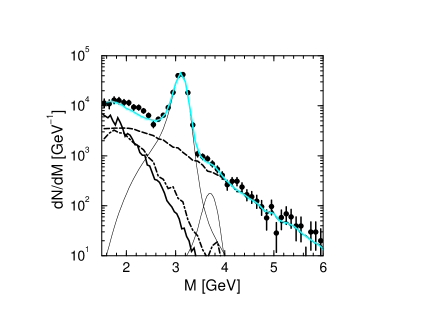
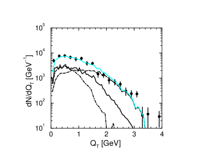
Figure 2: Comparison of our calculations with NA50 data [25]. Left panel: invariant mass distribution, right panel: $Q_{\perp}$ spectrum for the invariant mass bin $M=2.1\cdots 2.7$ GeV (solid curves: thermal contribution, dot-dashed curves: open charm, dashed curves: Drell-Yan, thin lines: parametrizations of the $J/\psi$ and $\psi^{\prime}$ contributions according to [25], gray curves: sum of these contributions).

The resulting invariant mass and transverse momentum spectra, including the thermal source contribution, are displayed in Fig. 2. The thermal source, with parameters $T_{\rm eff}$ and $N_{\rm eff}$ adjusted to the above CERES data, is needed to achieve the overall agreement with data. This unifying interpretation of different measurements has to be contrasted with other proposals of explaining the dimuon excess in the intermediate mass region either by final state hadron interactions [14] or by an abnormally large open charm enhancement [25]. The latter one should be checked experimentally [31] thus attempting a firm understanding of dilepton sources. Notice that our minimum parameter model describes the data equally well as the more detailed dynamical models [10, 11].

3.2 Sulfur beam data

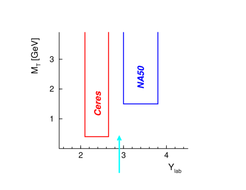
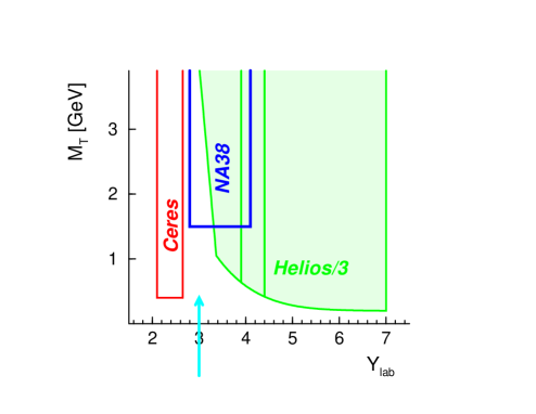
Figure 3: Coverage of the rapidity $Y_{\rm lab}$ and transverse mass $M_{\perp}$ of the various dilepton experiments. (a) left panel: lead beam, (b) right panel: sulfur beam. The arrows indicate the $pp$ center-of-mass rapidity.

Let us now turn to the older sulfur beam data (cf. [6] for a recent survey on models and an extensive reference list). Since a much larger rapidity interval is covered (see Fig. 3) we smear the source distribution (3) by a Gaussian function with a width of $\sigma=0.8$, i.e.

$$\frac{dN}{d^{4}Q}=\frac{5\alpha^{2}}{36\pi^{4}}N_{\rm eff}\int\frac{dY^{\prime}}{\sqrt{2\pi\sigma^{2}}}\exp\left\{-\frac{M_{\perp}\cosh(Y-Y^{\prime})}{T_{\rm eff}}\right\}\exp\left\{\frac{(Y^{\prime}-Y_{\rm cms})^{2}}{2\sigma^{2}}\right\}.$$ (5)

For $Y_{\rm cms}$ we choose 2.45 as suggested by an analysis of the rapidity distribution of negatively charged hadrons from NA35 [32] as displayed in Fig. 4. The width of the dilepton source, $\sigma$, is somewhat smaller than the width of the hadron distribution, cf. Fig. 4. Here we neglect also the small differences of the various target nuclei (Au, U, W) and attempt a unique parametrization of the $e^{-}e^{+}$ and $\mu^{-}\mu^{+}$ channels.

3.2.1 CERES experiment

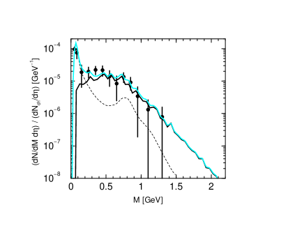
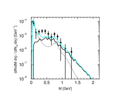
Figure 5: Comparison of our model calculations with the CERES data [33] with separately adjusted normalization factor $N_{\rm eff}=11.2\times 10^{4}$ fm⁴ (left panel) or with normalization $N_{\rm eff}=5.3\times 10^{4}$ fm⁴ adjusted to HELIOS/3 data [37] (right panel). Dashed curves: hadronic cocktail from [33], solid curves: thermal yield, gray curves: sum.

For the CERES $e^{+}e^{-}$ data [33] in central S(200 AGeV) + Au reactions, corresponding to $\langle\frac{dN_{ch}}{d\eta}\rangle=125$, the published hadronic cocktail is used. The acceptance is the same as described in subsection 3.1.1. The comparison of our calculations with the data is displayed in Fig. 5. A good description of the data is achieved by $T_{\rm eff}=160$ MeV. One observes in the left pannel of Fig. 5 indeed a fairly well reproduction of the spectral shapes for the choice of the normalization factor $N_{\rm eff}=11.2\times 10^{4}$ fm⁴. (Notice that this normalization factor is ununderstandably large. We focus here, however, on the shape of the spectra and do not attempt a change of our simple parametrization to resolve this issue, e.g. by employing another rapidity distribution. In this context we mention the second reference in [22] where, within the same transport code, the lead beam data [20] are satisfactorily reproduced but the sulfur beam data [33] strongly underestimated. Similarily, if we use the same normalization factor, as adjusted to the HELIOS/3 data (see subsection 3.2.3 below) our resulting spectrum is below the data and even outside of the systematical error bars at $M\sim 400$ MeV, see right pannel of Fig. 5.)

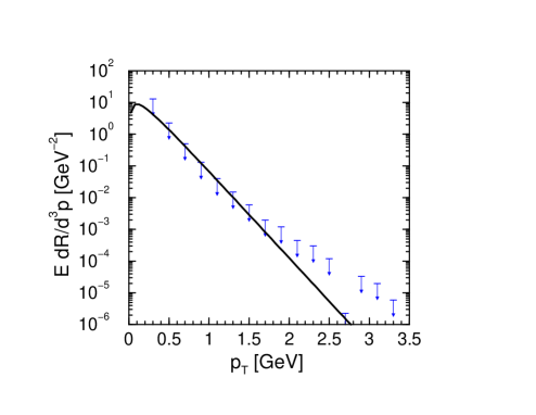
Figure 6: A comparison of the thermal photon spectrum (without transverse matter flow) with the experimental upper bounds [34] when adjusting the source strength to the HELIOS/3 data [37].

We mention additionally that adjusting the normalization to the HELIOS/3 data [37] the published upper bounds of the direct photon yields [34] are just compatible with our model calculations when adopting the model described in section 2 for photons [24] (see Fig. 6). In contrast, when choosing the normalization, which delivers an optimum description of the CERES data, one would be above the upper photon bounds in [34].

3.2.2 NA38 experiment

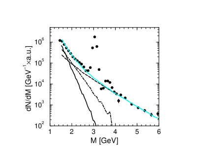
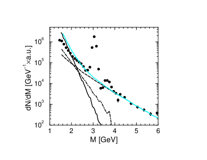
Figure 7: Comparison of our model calculations with the NA38 data [35] with separately adjusted normalization factor $N_{\rm eff}=21.3\times 10^{4}$ fm⁴ (left panel) and with normalization $N_{\rm eff}=5.3\times 10^{4}$ fm⁴ adjusted to HELIOS/3 data [37] (right panel). Meaning of the curves: thermal yield, open charm contribution and Drell-Yan (from left to right at larger $M$); gray curves: sum of all contributions;

The acceptance of this dimuon experiment is described by $Y_{\rm lab}=2.8\cdots 4.1$ and $|\cos\Theta_{\rm CS}|<0.5$. The comparison of our calculations with the NA38 data [35] for the reaction S(200 AGeV) + U in the intermediate-mass and high-mass region is displayed in Fig. 7. Adjusting the normalization factor to the data we achieve an optimum description by $N_{\rm eff}=1.3\times 10^{4}$ fm⁴ (left pannel), while the use of the normalization, adjusted to HELIOS/3 data, results in a unsatisfactory data description (right pannel in Fig. 7). It should be emphasized that all other data sets we are analyzing are for more restrictive central events. It is therefore clear that the required normalization factor for the NA38 data is smaller.

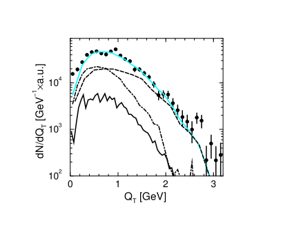
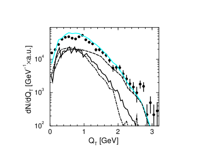
Figure 8: Comparison of our model calculations with the transverse momentum spectrum of dileptons from NA38 [35] in the intermediate-mass region $M=2.1\cdots 2.7$ GeV. Normalizations as in Fig. 7.

The available transverse momentum spectrum of NA38 is also nicely reproduced in shape (see Fig. 8).

Recently, the NA38/50 collaboration published also dilepton data in the low-mass region [36]. Since we have no reliable background contribution (hadronic cocktail) within the given acceptance at hand we discard the inclusion of these data in our analysis.

3.2.3 HELIOS/3 experiment

While we can nicely reproduce the Drell-Yan background for the HELIOS/3 experiment (cf. [37]), our PYTHIA simulations deliver another open charm contribution than the one used in previous analyses [5]. Since the accurate knowledge of the background contributions is necessary prerequisite, we use therefore for our analysis the difference $\mu^{+}\mu^{-}$ spectra of S(200 AGeV) + W and p(200 GeV) + W reactions [37], thus hoping to get rid of the background since these spectra are appropriately normalized. The centrality selection for these data is a multiplicity larger than 100 in the pseudo-rapidity bin $3.5\cdots 5.2$ resulting in an averaged multiplicity of 134.6 [37].

The acceptance is described by $M_{\perp}>max\left\{4(7-2Y_{\rm lab})\mbox{GeV},\sqrt{4m_{\mu}^{2}+\left(\frac{15{\mbox{{\small GeV}}}}{\cosh Y_{\rm lab}}\right)^{2}}\right\}$ and the data are binned in the rapidity intervals $Y_{\rm lab}=3.0\cdots 3.9,3.9\cdots 4.4,4.4\cdots 7.0$. It is in particular this wide rapidity span and the binning which require the Gaussian smearing of the dilepton source. Considering the rapidity-integrated yield, as done in most previous analyses when only the integrated data were at disposal, discards an important information and allows a unique description of the CERES lead beam data and HELIOS/3 sulfur beam data without any problem [38].

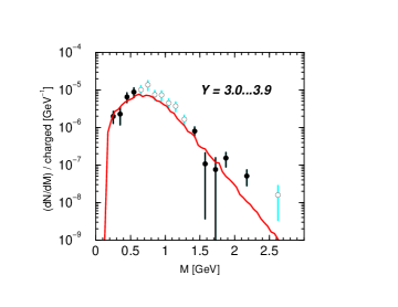
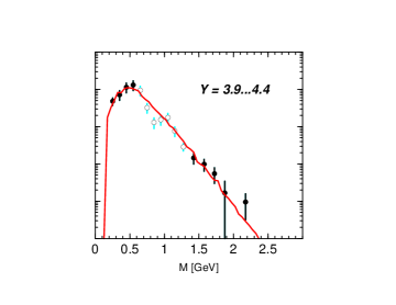
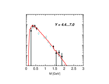
Figure 9: Comparison of our model calculations with the normalized HELIOS/3 difference data [S(200 A$\cdot$GeV) + W minus p(200 A$\cdot$GeV) + W] in various rapidity bins [37] with a unique normalization factor $N_{\rm eff}=5.3\times 10^{4}$ fm⁴. The black dots indicate data groups for which also $Q_{\perp}$ spectra are available (cf. Fig. 10).

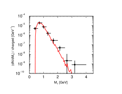
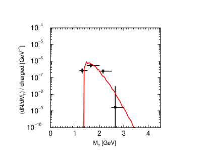
Figure 10: Comparison of our model calculations with the HELIOS/3 difference data [37] for the $M_{\perp}$ distributions with a unique normalization factor $N_{\rm eff}=2\times 5.3\times 10^{4}$ fm⁴ within the rapidity bin $Y_{\rm lab}=3.0\cdots 4.4$ for the invariant mass intervals $M=0.2\cdots 0.6$ GeV (left panel) and $M=1.35\cdots 2.5$ GeV (right panel). The additional factor 2 in the normalization is from a mismatch of these data compared with the ones in Fig. 9.

As seen in Fig. 9 the difference spectra in the various rapidity bins are fairly well described for $N_{\rm eff}=5.3\times 10^{4}$ fm⁴. (Notice that, in comparison with the lead beam data, also this normalization is quite large.) The $M_{\perp}$ spectra in the two available $M$ bins for the integrated rapidity bin $Y=3\cdots 4.4$ are also described in gross features, see Fig. 10. (Integrating the experimental $M_{\perp}$ spectra in this figure one finds a factor of 2 difference to the spectra in Fig. 9 when integrating these over the corresponding $M$ intervals. This is accounted for in the Fig. 10.)

4 Discussion of flow and time evolution effects

4.1 Flow effects

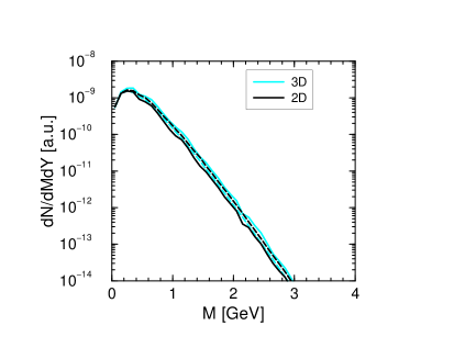
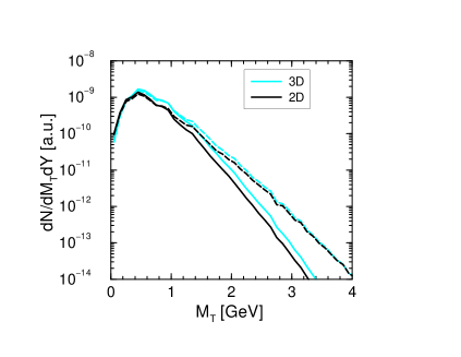
Figure 11: Sensitivity of the dilepton spectra at midrapidity against transverse flow within the blast wave model. Left panel: $dN/dM\,dY$, right panel: $dN/dM_{\perp}\,dY$. Solid curves: without transverse flow, dashed curves: with transverse flow $v_{\perp}=$ 0.6 (left panel) or 0.4 (right panel). The black (gray) curves are for a 2 (3) dimensional expansion (cf. [11] for further details).

As qualitatively discussed in [11] flow effects affect mainly the $Q_{\perp}$ or $M_{\perp}$ spectra. Explicit formulae for the dilepton spectra are given in [11] for (i) spherical expansion and (ii) longitudinally boost-invariant expansion superimposed on transverse expansion. In Fig. 11 we show the result of Monte Carlo simulations of the rates $dN/dM\,dY$ and $dN/dM_{\perp}\,dY$ at $Y=0$ for various values of the transverse flow velocity. One observes that the invariant mass spectra, delivered by a Monte Carlo procedure for generating the distribution Eq. (4), are indeed insensitive against flow (see Fig. 11, left panel). This is known for case (ii) for some time [39]. In contrast, the $Q_{\perp}$ spectra are sensitive against flow as demonstrated in the right panel of Fig. 11, in particular in the large-$Q_{\perp}$ region. However, as seen in Figs. 1 and 2, the large $Q_{\perp}$ region is dominated by the background contributions (hadronic cocktail or Drell-Yan). Therefore, one can indeed neglect the flow. Note that the key for this statement is a constraint on transverse flow from hadronic data. The analyzes of the $m_{\perp}$ spectra of several hadron species point to flow velocities $\langle v_{\perp}\rangle$ in the range from 0.43 c [2, 4] to 0.55 c [3]. Since the flow is expected to increase continuously with time due to acceleration from pressure, the transverse flow of hadrons at kinetic freeze-out is a temporal maximum value. The spatial and timewise average of the flow, relevant for dilepton and photon emission, must be smaller than the quoted values.

The situation may change at RHIC and LHC, where higher initial temperatures, and consequently larger pressures, cause a stronger transverse flow which could be manifest in dilepton $Q_{\perp}$ spectra.

4.2 Time evolution effects

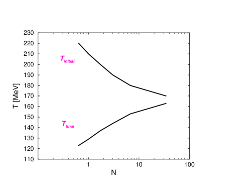
Figure 12: The change of the initial and final temperatures as a function of the normalization factor $N$.

Let us now discuss time evolution effects. As an example we show in Fig. 12 such initial temperatures and the corresponding final temperatures as a function of an normalization factor, $N$, which deliver the same invariant mass spectra in the range covered by the CERES and NA50 lead beam experiments displayed in Figs. 1 and 2. In calculating the curves in Fig. 12 the time evolution according to $T=T_{\infty}+(T_{\rm initial}-T_{\infty})\exp\left\{-\frac{t}{t_{2}}\right\}$, $V(t)=N\frac{A+B}{2.5n_{0}}\exp\left\{\frac{t}{t_{1}}\right\}$, with $T_{\infty}=110$ MeV, $t_{1}=5$ fm/c, $t_{2}=8$ fm/c is used as in [11] (cf. [40]), where $A,B$ are the mass numbers of the colliding nuclei, $n_{0}=0.17$ fm^-3. The temperature evolution starts at $T_{\rm initial}$ and is stopped at $T_{\rm final}$. (Such a temperature and volume evolution have been used first in [7] to show that the superposition of the thermal $q\bar{q}$ annihilation rate and the hadronic cocktail reproduces the shape of the CERES data obtained with the sulfur beam [33].) From Fig. 12 one can infer that, if the final temperature $T_{\rm final}$ is identified with the hadron kinetic freeze-out temperature of, e.g., 125 MeV according to [2], the corresponding initial temperature $T_{\rm initial}$ would be 215 MeV. This statement, however, depends on the assumed temperature evolution. For instance, in case of a bag model equation of state a different weighting would occur and therefore different values of the initial and final temperatures would follow. Nevertheless, the merging of the initial and final temperatures, $T_{\rm initial}$ and $T_{\rm final}$, at 170 MeV, displayed in Fig. 12, suggests to use only $T_{\rm eff}$ and $N_{\rm eff}$ instead of more parameters. Indeed, the above time evolution equations and the values displayed in Fig. 12 reproduce the value of $N_{\rm eff}=\int dt\,V(t)$ as used in subsection 3.1.

5 Summary

An attempt is reported to explain nearly the whole set of the dilepton data in recent CERN-SPS experiments with heavy-ion beams. We assume that the dilepton emissivity is the same as that in $q\bar{q}$ annihilation. This hypothesis is made to work in the low mass region and in the intermediate mass region possibly for different reasons. Whether several channels add up to smooth out a spectrum with intrinsic structure (“kinematical saturation”) or whether those structure are broadened and washed out is not addressed here. Note that while we find a good overall reproduction of the shapes of the experimental spectra, only the lead beam data can be explained with a unique and reasonable normalization.

As main result we emphasize that the average temperature of $T_{\rm eff}=160\cdots 170$ MeV used in this study is in good agreement with the temperature deduced from measured hadron ratios [1]. Since $T_{\rm eff}$ is an average, one can conclude that the achieved maximum temperatures are above this value and, therefore, in a region where deconfinement is expected according to lattice QCD calculations [41], which presently advocate a deconfinement temperature of $T_{c}=170$ MeV or somewhat larger.

In the present work we restrict ourselves to central collisions (except for the NA38 data) and compare several experiments with $e^{+}e^{-}$ and $\mu^{+}\mu^{-}$ channels. On the basis of this study an analysis of the $E_{\perp}$ dependence of the combined NA38 and NA50 data seems feasible. This is of interest since, due to the impact parameter dependence, some interpolation from lead beam data to sulfur beam data is desirable.

Our study is not a substitute for a detailed dynamical analysis. It is rather meant as a baseline calculation, designed to point out the underlying and unifying features of the experimental data, and to eventually extract a simpler physical message. We encourage dynamical microscopic prescriptions to attempt the global study performed here.

With respect to the recent heavy-ion experiments at CERN-SPS with lower beam energies (40 AGeV) an interesting question is whether the featureless $q\bar{q}$ spectrum is compatible with the upcoming data.

Acknowledgments

Stimulating discussions with W. Cassing, L. Capelli, O. Drapier, A. Drees, V. Koch, M. Mazera, R. Rapp, E. Scomparin, and G. Zinovjev are gratefully acknowledged. O.P.P. thanks for the warm hospitality of the nuclear theory group in the Research Center Rossendorf. The work is supported by BMBF 06DR921, WTZ UKR-008-98 and STCU-015.

Appendix A Background contributions

Since we compose the dilepton spectra of incoherently added thermal and background contributions one has carefully to check the reliability of the background estimates. We employ here the event generator PYTHIA [26] (version 6.104) for $pp$ collisions and scale the results to $AB$ collisions. Particular care has to be taken with the K factors. We use the parton distribution function set MRS D-’.

A.1 Drell-Yan

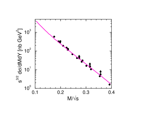
Figure 13: A comparison of the Drell-Yan cross section delivered by PYTHIA (with K factor as described in text) with the data [27].

In Fig. 13 a data compilation of the Drell-Yan cross sections [27] as a function of the scaling variable $M/\sqrt{s}$ and our PYTHIA simulations are displayed. The appropriate K factor is ${\cal K}_{\rm DY}=1.2$. Notice, however, that these data samples are for different beam energies and display a slight breaking of the anticipated scaling. Instead, independent fits of the invariant mass distributions of the data from [27, 28] deliver an averaged K factor of 1.5.

The intrinsic transverse parton momentum distribution can be fixed by the dilepton $Q_{\perp}$ spectrum in the Drell-Yan region $M>4.2$ GeV. A comparison with the NA38 data [35] delivers a value of $\langle k_{\perp}^{2}\rangle=(0.8\,\mbox{GeV})^{2}$ (see Fig. 14). We use in all calculations (also for charm) this value. The K factor is less affected by variations of $\langle k_{\perp}^{2}\rangle$.

A.2 Open charm

We use here PYTHIA with charm mass parameter $m_{c}=1.5$ GeV and default fragmentation ”hybrid”. There are two different sources of a determination of the open charm K factor. Either one uses the hadronic channels, i.e. cross sections of identified $D^{0}$ and $D^{+}$ mesons from Fermi lab experiments, which are compiled in [29], or the NA50 dilepton data [30] for the reaction p(450 GeV) + W. Fig. 15 shows the comparison with hadron channels, which deliver K factors of ${\cal K}_{D^{0}}=5.4$ and ${\cal K}_{D^{+}}=6.8$ resulting in an averaged open charm K factor of ${\cal K}_{c}=5.7$. Obviously these data do not constrain the K factor very reliably. A sharper constraint is given by the dilepton channel which confirms this value as seen in Fig. 16. The uncomfortably large K factor points to higher order processes which, however, could change the spectral shapes. In this respect the envisaged experiments by the NA60 collaboration [31] to identify explicitly open charm are very important for this dilepton source.

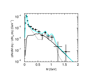
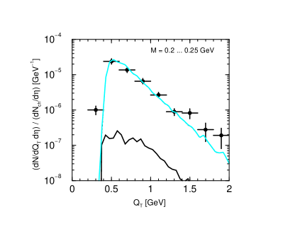
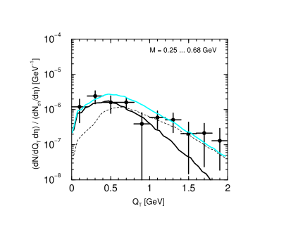
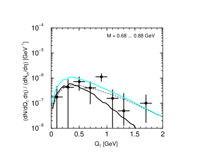
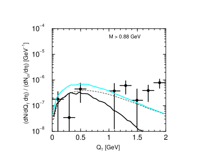
Figure 1: Comparison of our model with the preliminary CERES data [20]. Upper middle panel: invariant mass distribution, lower four panels: $Q_{\perp}$ spectra for various invariant mass bins (dashed lines: hadronic cocktail, solid curves: thermal yield, gray curves: sum).

Figure 4: A Gaussian fit to the NA35 data of negatively charged hadrons [32]. The arrow indicates the center of the Gaussian which has a width of $\sigma_{h^{-}}=1.1$.

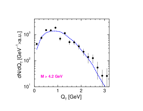
Figure 14: Unnormalized transverse momentum distribution of dileptons in the Drell-Yan region, $M>4.2$ GeV, in the NA38 experiment [35]. The solid curve is our result from PYTHIA simulations with $\langle k_{\perp}^{2}\rangle=(0.8\,\mbox{GeV})^{2}$. A value of $\langle k_{\perp}^{2}\rangle=(1\,\mbox{GeV})^{2}$, as implemented in the recent PYTHIA version 6.143, results in an apparently worse description of the data.

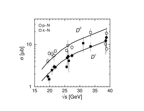
Figure 15: A comparison of the open charm cross section (data compilation from [29]) with our PYTHIA calculations (with K factors as described in text).

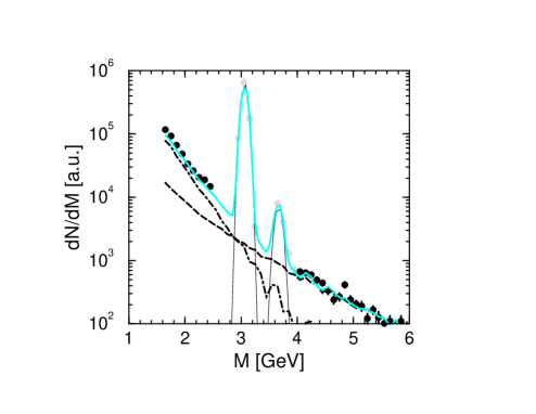
Figure 16: A comparison of our PYTHIA calculations with the dilepton spectrum in p(450 GeV) + W reactions [30]. Dashed curve: Drell-Yan, dot-dashed curve: open charm contribution, gray curve: sum of all contributions. Included are parametrizations of the $J/\psi$ and $\psi^{\prime}$ contributions according to [30].

References

-
[1]
P. Braun-Munzinger, J. Stachel, J.P. Wessels,
N. Xu, Phys. Lett. B 344 (1995) 43, B 365 (1996) 1,
J. Cleymans, K. Redlich, Phys. Rev. Lett. 81 (1998) 5284,
P. Braun-Munzinger, I. Heppe, J. Stachel, Phys. Lett. B 465 (1999) 15. -
[2]
B. Kämpfer, O.P Pavlenko, A. Peshier, M. Hentschel,
G. Soff, J. Phys. G 23 (1997) 2001c,
B. Kämpfer, hep-ph/9612336. - [3] B. Tomasik, U.A. Wiedemann, U. Heinz, nucl-th/9907096, and Nucl. Phys. A 663 (2000) 753c.
- [4] E.L. Bratkovskaya, W. Cassing, C. Greiner, M. Effenberger, U. Mosel, A. Sibirtsev, Nucl. Phys. A 675 (2000) 661.
- [5] G.Q. Li, C. Gale, Phys. Rev. C 58 (1998) 2914, Phys. Rev. Lett. 81 (1998) 1572.
- [6] R. Rapp, J. Wambach, hep-ph/9909229, Adv. Nucl. Phys. in print.
-
[7]
F. Klingl, W. Weise, hep-ph/9802211,
F. Klingl, Ph.D. thesis Munich 1998. - [8] Z. Huang, Phys. Lett. B 361 (1995) 131.
- [9] A.V. Leonidov, P.V. Ruuskanen, Eur. Phys. J. C 4 (1998) 519.
- [10] R. Rapp, E. Shuryak, Phys. Lett. B 473 (2000) 13.
- [11] K. Gallmeister, B. Kämpfer, O.P. Pavlenko, Phys. Lett. B 473 (2000) 20.
- [12] R.A. Schneider, W. Weise, hep-ph/0008083.
- [13] C. Spieles, L. Gerland, N. Hammon, M. Bleicher, S.A. Bass, H. Stöcker, W. Greiner, C. Lourenco, R. Vogt, Eur. Phys. J. C 5 (1998) 349.
- [14] Z. Lin, X.N. Wang, Phys. Lett. B 444 (1998) 245.
- [15] B. Kämpfer, O.P. Pavlenko, Phys. Lett. B 289 (1992) 127.
- [16] A. Peshier, M. Thoma, Phys. Rev. Lett. 84 (2000) 841.
- [17] B. Kämpfer, O.P. Pavlenko, A. Peshier, G. Soff, Phys. Rev. C 52 (1995) 2704.
- [18] P. Aurenche, F. Gelis, R. Kobes, H. Zaraket, Phys. Rev. D 60 (1999) 076002.
- [19] H. Nadeau, J. Kapusta, P. Lichard, Phys. Rev. C 45 (1992) 3034.
-
[20]
S. Esumi (for the CERES collaboration),
Proc. 15th Winter Workshop on Nuclear Dynamics, Jan. 1999, Park City,
B. Lenkeit, Nucl. Phys. A 661 (1999) 23c; Ph. D. thesis, Heidelberg 1998. - [21] R. Rapp, J. Wambach, Eur. Phys. J. A 6 (1999) 415.
-
[22]
V. Koch, C. Song, Phys. Rev. C 54 (1996) 1903,
V. Koch, nucl-th/9903008. - [23] Aggarwal et al. (WA98), nucl-ex/000606, nucl-ex/000607.
- [24] K. Gallmeister, B. Kämpfer, O.P. Pavlenko, Phys. Rev. C 62 (2000) 057901.
-
[25]
E. Scomparin (for the NA50 Collaboration),
Nucl. Phys. A 610 (1996) 331c, J. Phys. G 25 (1999) 235c,
P. Bordalo et al. (NA50), Nucl. Phys. A 661 (1999) 538c. - [26] T. Sjöstrand, Comp. Phys. Commun. 82 (1994) 74.
-
[27]
D.M. Kaplan et al., Phys. Rev. Lett. 40 (1978) 435,
A.S. Ito et al., Phys. Rev. D 23 (1981) 604,
C.N. Brown et al., Phys. Rev. Lett. 63 (1989) 2637. -
[28]
J. Badier et al., Z. Phys. C 26 (1985) 489
P.L. McGaughey et al., Phys. Rev. D 50 (1994) 3038. - [29] P. Braun-Munzinger, D. Miskowiec, A. Drees, C. Lorenco, Eur. Phys. J. C 1 (1998) 123.
- [30] L. Capelli, Talk at CERN–Workshop ’Charm Production in Nucleus Nucleus Collisions’, Dec. 2–3, 1999, http://www.cern.ch/NA50/papers.html.
- [31] C. Cicalo et al. (NA60), Letter of Intent, CERN/SPSC 99-15, SPSC/I221, May 1999.
- [32] T. Alber et al. (NA35), Eur. Phys. J. C 2 (1998) 643.
- [33] G. Agakhiev et al. (CERES), Phys. Rev. Lett. 75 (1995) 1272.
- [34] R. Albrecht et al. (WA80), Phys. Rev. Lett. 77 (1996) 2392.
- [35] M.C. Abreu et al. (NA38), Phys. Lett. B 423 (1998) 207.
- [36] M.C. Abreu et al. (NA38 and NA50), Eur. Phys. J. C 13 (2000) 69.
- [37] A.L.S. Angelis et al. (HELIOS/3), Eur. Phys. J. C 13 (2000) 433.
- [38] W. Cassing, E.L. Bratkovskaya, R. Rapp, J. Wambach, Phys. Rev. C 57 (1998) 916.
- [39] K. Kajantie, M. Kataja, L. McLerran, P.V. Ruuskanen, Phys. Rev. D 34 (1986) 811.
- [40] R. Rapp, G. Chanfray, J. Wambach, Nucl. Phys. A 617 (1997) 472.
- [41] F. Karsch, Nucl. Phys. Proc. Suppl. 83-84 (2000) 14.