JYFL-5/00

hep-ph/0010319

20 October, 2000

TRANSVERSE ENERGY FROM MINIJETS
IN ULTRARELATIVISTIC NUCLEAR COLLISIONS:
A NEXT-TO-LEADING ORDER ANALYSIS

K.J. Eskola^a,b and K. Tuominen^a

^a Department of Physics, University of Jyväskylä,
P.O.Box 35, FIN-40351, Jyväskylä, Finland
^b Helsinki Institute of Physics,
P.O.Box 9, FIN-00014, University of Helsinki, Finland

Abstract

We compute in next-to-leading order (NLO) perturbative QCD the amount of transverse energy produced into a rapidity region $\Delta Y$ of a nuclear collision from partons created in the few-GeV subcollisions. The NLO formulation assumes collinear factorization and is based on the subtraction method. We first study the results as a function of the minimum transverse momentum scale and define and determine the associated $K$-factors. The dependence of the NLO results on the scale choice and on the size of $\Delta Y$ is also studied. The calculations are performed for GRV94 and CTEQ5 sets of parton distributions. Also the effect of nuclear shadowing to the NLO results is investigated. The main results are that the NLO results are stable relative to the leading-order (LO) ones even in the few-GeV domain and that there exists a new kinematical region not present in the LO, which is responsible for the magnitude of the $K$-factors. The dependence on the size of $\Delta Y$ is found to be practically linear within two central units of rapidity, and the scale dependence present at RHIC energies is seen to vanish at the LHC energies. Finally, the effect of NLO corrections to the determination of transverse energies and multiplicities in nuclear collisions is discussed within the framework of parton saturation.

1 Introduction

The heavy ion community experiences currently a new exciting period as the first data in ultrarelativistic heavy ion collisions at BNL-RHIC are being analysed and the first physics results are coming out. These include the observation by the PHOBOS collaboration of an increased activity in Au+Au collisions at $\sqrt{s}=56$ and $130\,A{\rm GeV}$ [1]: the number of charged particles per participant pair clearly increases from that in Pb+Pb collisions at the CERN-SPS at $\sqrt{s}=17.3\,A{\rm GeV}$, and from $p\bar{p}$ at $\sqrt{s}=50\dots 200$ GeV. This lends support to a description of initial particle production in high energy heavy ion collisions in terms of binary collision mechanisms. The first results from the STAR collaboration have in turn shown an increase of elliptic flow in Au+Au at $\sqrt{s}=130\,A{\rm GeV}$, observed as an enhanced asymmetry in the azimuthal distributions of particles [2]. This points towards collectivity, pressure and thermalization in the produced system.

A complete description of a collision of two heavy ions at high energy is clearly an extremely challenging task: elementary QCD-quanta, gluons, quarks and antiquarks, are expected to be produced abundantly enough, so that they thermalize locally and form a new, deconfined phase of matter, the Quark Gluon Plasma (QGP). After its production the system will experience an expansion stage during which it will cool down and go through a phase transition from the QGP to a hadron gas. Eventually, decoupling sets in and the hadrons fly independently to the detector, possibly decaying into other particles before that.

Due to our ignorance of how to solve nonperturbative QCD, calculations to describe such a complicated spacetime evolution are very difficult to do from truly first principles. Instead, the evolution can be effectively modelled in terms of relativistic hydrodynamics [3, 4], which relies on the assumption of a locally thermal system. The benefit in such an approach, in addition to simplicity, is a proper treatment of the phase transition and inclusion of collective effects (pressure and flow). The initial conditions, however, have to be given from outside. Alternatively, one may try to describe the strongly interacting system first as a cascade of partons [5, 6] and then as a hadronic cascade [7, 8], or, as recently suggested, as a combination of the hydrodynamical approach and a hadron cascade [9].

Common to the approaches mentioned above, the initial conditions, i.e. the energy densities and number densities of initially produced quarks and gluons, along with the formation times, need to be known as precisely as possible. As also the degree of thermalization of the QGP [10, 11, 12] depends heavily on the initial conditions, it is vitally important to study them in detail. In this paper we will do this by formulating and computing the initial transverse energy production from minijets in central $AA$ collisions to next-to-leading order (NLO) in perturbative QCD (pQCD).

Initial particle production in $AA$ collisions at collider energies has typically been described with two-component models where pQCD accounts for the hard and semihard scatterings of partons and a phenomenological model for the soft particle production [13, 14, 15, 16]. At sufficiently high cms-energies, partons produced with transverse momenta in the semihard domain, $p_{T}\geq p_{0}\sim 1\dots 2$ GeV, become the dominant source of energy deposited in central rapidities [13, 17, 18]. Within the leading twist framework the inclusive cross sections for production of semihard partons, along with the initial $E_{T}$ carried by them, are computable in terms of collinear factorization [19] of pQCD [18, 13]. Individual binary scatterings of partons (or nucleons) are assumed to be independent of each other and nuclear effects can be included by using nuclear parton distributions [20]. Computation of the pQCD component thus leans on the fact that production of quarks and gluons is reliably described by pQCD at large transverse momentum scales, where it is possible to actually observe individual jets in $pp$ collisions. The main uncertainties are related to the determination of the semihard scale $p_{0}$ defining the perturbative component, and to the higher order contributions to the parton cross sections. To reduce the latter source of uncertainty is the main motivation for the present NLO study.

The studies [13, 14, 15, 17] are in practise extensions from the $pp\,(p\bar{p})$ physics in the sense that the smallest transverse momentum included in the perturbative component, $p_{0}$, is constrained by data from hadronic physics and kept constant in the extrapolation to $AA$. Recently, however, ideas of parton saturation [18, 21] have been revived for an effective estimation of the initial gluon and quark production based on the pQCD component [22, 23] alone. The perturbative production of partons is extendend down to a minimum scale $p_{0}=p_{\rm sat}$, defined as the scale at which the produced partons, each of which is of the size $\pi/p_{0}^{2}$, effectively fill the available transverse area $\pi R_{A}^{2}$. This is the simplest way of defining a saturation criterion in central $AA$ collisions. For $A\sim 200$, this procedure leads to $p_{\rm sat}\sim 1$ GeV for RHIC energies $\sqrt{s}=56\dots 200\,A{\rm GeV}$ and $p_{\rm sat}\sim 2$ GeV for the LHC energy $\sqrt{s}=5500\,A{\rm GeV}$ [22]. The criterion which determines when the system becomes saturated, may contain nonperturbative, even phenomenological features. Terminating the pQCD computation at $p_{0}=p_{\rm sat}(\sqrt{s},A)$ thus gives an estimate of the total initial parton production. The effective formation time of the minijet (gluon) plasma system is then obtained as $\tau_{0}\sim 1/p_{\rm sat}$. The determination of $p_{\rm sat}$ in the pQCD+saturation approach is a dynamical procedure which is affected by the NLO contributions to partonic cross sections. Again, reducing the uncertainty related to the higher order contributions in minijet production is the general goal in this paper.

Another promising approach for describing initial gluon production is that of classical fields [24]. The gluon fields originate from colour sources moving along the light cones and, assuming longitudinal boost-invariance, an effective dimensionally reduced Hamiltonian can be formed and the gluon production computed through a lattice simulation [25]. Interestingly, also in these classical field computations gluons with fairly hard momenta $E_{T}/N\sim 3Q_{\rm sat}$, where $Q_{\rm sat}$ is a similar saturation scale as $p_{\rm sat}$ above, are important for the initial production [26, 27]. As this approach should coincide with the perturbative one in the limit of high transverse momentum of produced gluons, it is important to reduce the uncertainties related to the possible higher-order contributions in the pQCD component. This gives further motivation to perform the NLO computation of initial $E_{T}$ we present in this paper.

In our study the NLO evaluation of the produced initial transverse energy in central ($b=0$) $AA$ collisions is carried out by computing the first $E_{T}$ moment $\sigma_{\rm QCD}\langle E_{T}\rangle_{\Delta Y,p_{0}}$ of the perturbative $E_{T}$ distribution of minijets in a single proton-proton collision within the framework of collinear factorization. Nuclear collision geometry is taken into account through the standard nuclear overlap functions $T_{AA}({\bf b})$ and the initial $E_{T}$ is obtained as $E_{T}=T_{AA}\sigma_{\rm QCD}\langle E_{T}\rangle$ [13]. The parameter $p_{0}$ defines the extent of the perturbative treatment: we include all hard scatterings of partons in which at least an amount of $2p_{0}$ of transverse momentum is created. Note that $p_{0}\gg\Lambda_{\rm QCD}$ is kept as an external parameter, allowing for different phenomenological ways to determine its value.

We emphasize that although the initial $E_{T}$ in a rapidity acceptance window $\Delta Y$ is a physical quantity, which thus can be computed in an infrared safe manner, it is not a direct observable. This is due to the interactions of initially produced gluons and quarks which are expected to thermalize the QGP system rapidly. Due to the pressure $P$ formed, the system does work ($PdV$) during the expansion stage, and some of the initially stopped energy is lost. In ref. [22] it was estimated that for central collisions of $A\sim 200$ the measurable final state $E_{T}$ is $E_{T}^{\rm initial}/3$ at the highest RHIC energy and $E_{T}^{\rm initial}/5$ at the LHC energy.

In practise, the NLO computation is performed by appealing to a subtraction algorithm [28, 29, 30], applicable for a wide class of problems requiring a NLO evaluation of a quantity fulfilling the requirements of infrared safeness. The required $\mathcal{O}(\alpha_{s}^{3})$ matrix elements have been evaluated in [31]. The current paper is a sequel to our previous work [32], where $\sigma_{\rm QCD}\langle E_{T}\rangle_{\Delta Y,p_{0}}$ was computed numerically and the results studied as a function of the parameter $p_{0}$ and the factorization/renormalization scale choice. The main result of [32], that the deviation of the NLO results from the LO ones are not dramatically increasing as $p_{0}$ is taken down from $10$ GeV to $1\dots 2$ GeV, remains also here. In [32] it was noted that a new and important kinematical perturbative region has to be included in the NLO computation. Here we study the contributions from this region in more detail. The relation to another recent NLO computation of the initial $E_{T}$, Ref. [33], along with the differences from our formulation, were also discussed in [32]. Now we extend the NLO study to explore the sensitivity of the results on the choice of parton distributions. In addition to the dependence of the results on $p_{0}$ and on the scale choice, their dependence on $\Delta Y$ is explicitly shown and the important implications discussed. Also the effects of nuclear parton distributions [20] are studied. Finally, as an application of the NLO computation, charged particle production for the nucleus-nucleus collisions currently under way at RHIC as well as for those to take place in the future at the LHC/ALICE are briefly considered by applying the pQCD+saturation model [22].

2 Theoretical basis of the NLO formulation

In the framework of independent parton-parton scatterings, the average $E_{T}$ produced initially into the rapidity region $\Delta Y$ in an $AA$ collision at an impact parameter ${\bf b}$ can be computed as [13]

$$E_{T}^{AA}({\bf b},\sqrt{s},p_{0})=T_{AA}({\bf b})\sigma_{\rm QCD}\langle E_{T}\rangle_{\Delta Y,p_{0}},$$ (1)

where $T_{AA}(\bf b)$ is the standard nuclear overlap function [13]. We will focus on central collisions of large nuclei only, for which, using the Woods-Saxon nuclear profiles, $T_{AA}(0)\approx A^{2}/\pi R_{A}^{2}$. Numerically, $T_{AA}(0)\approx 30/$mb for $A\sim 200$. In what follows, we will focus on the formulation and computation of $\sigma_{\rm QCD}\langle E_{T}\rangle_{\Delta Y,p_{0}}$, the first moment of the minijet $E_{T}$ distribution in $pp$ collisions. Regarding the $E_{T}$ distribution in an $AA$-collision, it is the first and also the second moments of the $pp$-level distributions that play the key roles rather than the distributions themselves [13].

Calculation of physical cross sections in NLO pQCD is a nontrivial task even if the scattering amplitudes are known at the desired order. For infrared safe quantities, however, a systematic method allowing for the cancellation of the soft and collinear singularities in the loop and bremsstrahlung contributions exists [30, 34]. In this section we will briefly review this algorithm and thoroughly describe its implementation.

2.1 Subtraction method

To order $\alpha_{s}^{3}$ we need to take into account processes where two incoming hadrons produce either two or three final state partons. Keeping the notations of [30], the incoming partons are labelled by $A$ and $B$ and the outgoing partons as 1, 2 and 3. For the two-parton final state the appropriate kinematical variables are $y_{1},y_{2},p_{T2}$ and $\phi_{2}$. Transverse momentum conservation determines $p_{T1}=p_{T2}=p_{T}$ and $\phi_{1}=\phi_{2}+\pi$ as we do not include any intrinsic transverse momentum. The momentum fractions $x_{A}$ and $x_{B}$ of the incoming partons are determined by the conservation of energy and longitudinal momentum, resulting in $x_{1,2}=\frac{p_{T}}{\sqrt{s}}({\rm e}^{\pm y_{1}}+{\rm e}^{\pm y_{2}})$. Similarly, for the three-parton final state ${\bf p_{T1}}=-({\bf p_{T2}+p_{T3}})$ and the suitable kinematical variables are $y_{1},y_{2},y_{3},p_{T2},p_{T3},\phi_{2}$ and $\phi_{3}$. The fractional momenta become now $x_{1,2}=\frac{p_{T1}}{\sqrt{s}}{\rm e}^{\pm y_{1}}+\frac{p_{T2}}{\sqrt{s}}{\rm e}^{\pm y_{2}}+\frac{p_{T3}}{\sqrt{s}}{\rm e}^{\pm y_{3}}$. An inclusive hard cross section can be written in a general form

$$I = \int d[PS]_{2}\frac{d\sigma^{2\rightarrow 2}}{d[PS]_{2}}S_{2}(p_{1}{{}^{\mu}},p_{2}^{\mu})+\int d[PS]_{3}\frac{d\sigma^{2\rightarrow 3}}{d[PS]_{3}}S_{3}(p_{1}^{\mu},p_{2}^{\mu},p_{3}^{\mu})$$ (2)

$$\equiv I[2\rightarrow 2]+I[2\rightarrow 3],$$

where it is implicit that the integrations take place in $4-2\epsilon$ spacetime dimensions. To condense the notation, we have denoted the $2\rightarrow 2$ and $2\rightarrow 3$ differential partonic cross sections as

$$\frac{d\sigma^{2\rightarrow 2}}{d[PS]_{2}}=\frac{d\sigma^{2\rightarrow 2}}{dp_{T}dy_{1}dy_{2}d\phi_{2}}$$ (3)

$$\frac{d\sigma^{2\rightarrow 3}}{d[PS]_{3}}=\frac{d\sigma^{2\rightarrow 3}}{dp_{T2}dp_{T3}dy_{1}dy_{2}dy_{3}d\phi_{2}d\phi_{3}},$$ (4)

which also defines our notation for the phase space volume elements $d[PS]_{2}$ and $d[PS]_{3}$.

The measurement functions $S_{2}(p_{1}^{\mu},p_{2}^{\mu})$ and $S_{3}(p_{1}^{\mu},p_{2}^{\mu},p_{3}^{\mu})$ which depend on the four-momenta of the final state partons, define the physical quantity the cross section of which is to be computed. Such a quantity can be e.g. a differential one-jet cross section $\frac{d\sigma}{dp_{T}dy}\big{|}_{R}$ [28, 30], or a two-jet cross section $\frac{d\sigma}{dp_{T1}dp_{T2}dy_{1}dy_{2}}\big{|}_{R}$ [35] for production of observable jets with a jet cone radius $R$. In our case, $S_{2}$ and $S_{3}$ will be designed to give $\frac{d\sigma}{dE_{T}}\big{|}_{\Delta Y,p_{0}}$, the differential $E_{T}$ distribution of minijets which fall into a given rapidity acceptance window $\Delta Y$ and which originate from perturbative collisions where at least an amount $2p_{0}$ of transverse momentum is produced.

Let us briefly recapitulate the procedure presented in detail in [30] for the cancellation of singular contributions in the above cross section. The $2\rightarrow 2$ contribution can be written under collinear factorization [19] as

$$\frac{d\sigma^{2\rightarrow 2}}{d[PS]_{2}} = \frac{1}{2!}\sum_{a_{A},a_{B},a_{1},a_{2}}\frac{p_{T2}}{16\pi^{2}s^{2}}\frac{1}{x_{A}}\tilde{f}_{A}(a_{A},x_{A})\frac{1}{x_{B}}\tilde{f}_{B}(a_{B},x_{B})$$ (5)

$$\times\langle|\mathcal{M}(a_{A}+a_{B}\rightarrow a_{1}+a_{2})|^{2}\rangle S_{2}(p_{1}^{\mu},p_{2}^{\mu}).$$

The incoming parton flavors are denoted by $a_{A}$ and $a_{B}$ whereas the outgoing parton distributions are denoted by $a_{1}$ and $a_{2}$. The matrix element squared and summed over final spin and color and averaged over initial spins and colors is evaluated in $4-2\epsilon$ dimensions and contains the ultraviolet renormalization via the $\overline{\mbox{\rm MS}}$ scheme. The distributions $\tilde{f}(a,x)$ are the modified parton distributions defined in the $\overline{\mbox{\rm MS}}$ scheme.

Similarly for the $2\rightarrow 3$ part one has

$$\frac{d\sigma^{2\rightarrow 3}}{d[PS]_{3}} = \frac{1}{2!}\theta(p_{T3}<p_{T1})\theta(p_{T3}<p_{T2})\frac{p_{T2}p_{T3}}{8(2\pi)^{5}s^{2}}\sum_{a_{A},a_{B},a_{1},a_{2},a_{3}}\frac{1}{x_{A}}f_{A}(a_{A},x_{A})$$ (6)

$$\times\frac{1}{x_{B}}f_{B}(a_{B},x_{B})\langle|\mathcal{M}(a_{A}+a_{B}\rightarrow a_{1}+a_{2}+a_{3})|^{2}\rangle S_{3}(p_{1}^{\mu},p_{2}^{\mu},p_{3}^{\mu}),$$

where parton 3 has been identified as the one having smallest transverse momentum, canceling a factor 3 in the original statistical prefactor 1/3!.

The two terms, $I[2\rightarrow 2]$ and $I[2\rightarrow 3]$ both contain divergent contributions proportional to $1/\epsilon$ and $1/\epsilon^{2}$. All these divergent contributions cancel remarkably against each other provided that the functions $S_{2}$ and $S_{3}$ in the equation above, the so called measurement functions, are infrared safe. This requirement can be stated more precisely: First, as two of the outgoing partons become collinear, $S_{3}$ should reduce to $S_{2}$ i.e.

$$S_{3}(p_{1}^{\mu},(1-\lambda)p_{2}^{\mu},\lambda p_{2}^{\mu}) = S_{2}(p_{1}^{\mu},p_{2}^{\mu}),$$

$$S_{3}((1-\lambda)p_{1}^{\mu},p_{2}^{\mu},\lambda p_{1}^{\mu}) = S_{2}(p_{1}^{\mu}\,p_{2}^{\mu}),$$

$$S_{3}(\lambda p_{1}^{\mu},(1-\lambda)p_{1}^{\mu},p_{2}^{\mu}) = S_{2}(p_{1}^{\mu},p_{2}^{\mu})$$ (7)

for $0\leq\lambda\leq 1$. Second, as any of the partons becomes collinear with one of the beam momenta $p_{A}^{\mu}$, $p_{B}^{\mu}$ it is required similarly, that

$$S_{3}(p_{1}^{\mu},p_{2}^{\mu},\lambda p_{A}^{\mu}) = S_{3}(p_{1}^{\mu},p_{2}^{\mu},\lambda p_{B}^{\mu})=S_{2}(p_{1}^{\mu},p_{2}^{\mu}),$$

$$S_{3}(p_{1}^{\mu},\lambda p_{A}^{\mu},p_{2}^{\mu}) = S_{3}(p_{1}^{\mu},\lambda p_{B}^{\mu},p_{2}^{\mu})=S_{2}(p_{1}^{\mu},p_{2}^{\mu}),$$

$$S_{3}(\lambda p_{A}^{\mu},p_{1}^{\mu},p_{2}^{\mu}) = S_{3}(\lambda p_{B}^{\mu},p_{1}^{\mu},p_{2}^{\mu})=S_{2}(p_{1}^{\mu},p_{2}^{\mu})$$ (8)

Assuming the infrared safety of the measurement functions, the calculation based on the subtraction method [30] then proceeds by first separating the singular factors in $2\rightarrow 3$ matrix element from one another. As an initial step, the matrix element is decomposed as

$$\langle|\mathcal{M}|^{2}\rangle_{2\rightarrow 3}=\langle|\mathcal{M}|^{2}\rangle_{A}+\langle|\mathcal{M}|^{2}\rangle_{B}+\langle|\mathcal{M}|^{2}\rangle_{1}+\langle|\mathcal{M}|^{2}\rangle_{2}$$ (9)

in such a way that each term $\langle|\mathcal{M}|^{2}\rangle_{n}\sim 1/(p_{3}\cdot p_{n})$, so it contains a soft singularity for parton 3 along with the singularity of parton 3 becoming collinear with parton $n$, where $n=A,B,1,2$ with $A,B$ referring to the incoming partons and 1,2 to the two other outgoing partons. The imposed constraint $p_{T3}<p_{T1},p_{T2}$ guarantees that other singularities do not occur. Now the $2\rightarrow 3$ part of the cross section can be written as

$$I[2\rightarrow 3]=I[2\rightarrow 3]_{A}+I[2\rightarrow 3]_{B}+I[2\rightarrow 3]_{1}+I[2\rightarrow 3]_{2}.$$ (10)

Each of the four terms featured in the above equation can be treated independently and in a similar manner. For example, the last term becomes

$$I[2\rightarrow 3]_{2}=\int\frac{d\sigma^{2\rightarrow 3}_{2}}{d[PS]_{3}}{d[PS]_{3}}=\int{d[PS]_{3}}\frac{F_{2}(y_{1},p_{T2},y_{2},\phi_{2},p_{T3},y_{3},\phi_{3})}{p_{T3}[\cosh(y_{2}-y_{3})-\cos(\phi_{2}-\phi_{3})},$$ (11)

where the divergent factor $1/(p_{2}\cdot p_{3})$ has been expressed in terms of the integration variables as $p_{2}\cdot p_{3}=p_{T2}p_{T3}[\cosh(y_{2}-y_{3})-\cos(\phi_{2}-\phi_{3})]$, and $F_{2}$ is a complicated function containing the parton distributions, the measurement function $S_{3}$ and certain parts of the ($4-2\epsilon$ dimensional) squared matrix elements due to the decomposition in Eq. (9).

The aim is now to decompose $d\sigma^{2\rightarrow 3}_{2}/d[PS]_{3}$ into terms that are divergent but simple in a way that the integrations over the phase space of the third parton can be performed analytically and terms that are finite as $\epsilon\rightarrow 0$ but not so simple. This goal is achieved by inserting zero in the following clever manner:

$$F_{2}(y_{1},p_{T2},y_{2},\phi_{2},p_{T3},y_{3},\phi_{3})=$$

$$F_{2}(y_{1},p_{T2},y_{2},\phi_{2},p_{T3},y_{3},\phi_{3})-F_{2}(y_{1},p_{T2},y_{2},\phi_{2},0,y_{3},\phi_{3})\theta(p_{T3}<p_{T2}/2)$$

$$-F_{2}(y_{1},p_{T2},y_{2},\phi_{2},p_{T3},y_{2},\phi_{2})+F_{2}(y_{1},p_{T2},y_{2},\phi_{2},0,y_{2},\phi_{2})\theta(p_{T3}<p_{T2}/2)$$

$$+F_{2}(y_{1},p_{T2},y_{2},\phi_{2},0,y_{3},\phi_{3})\theta(p_{T3}<p_{T2}/2)$$

$$+F_{2}(y_{1},p_{T2},y_{2},\phi_{2},p_{T3},y_{2},\phi_{2})-F_{2}(y_{1},p_{T2},y_{2},\phi_{2},0,y_{2},\phi_{2})\theta(p_{T3}<p_{T2}/2).$$ (12)

The first four terms on the right-hand side combine to make up the term $I[{\rm{finite}}]_{2}$ which is perfectly finite as $\epsilon\rightarrow 0$ as both the soft singularity $p_{T3}=0$ and the collinear singularity $3\uparrow\uparrow 2$ have been subtracted. The fifth term, containing the soft singularity, generates a term $I[{\rm soft}]_{2}$, and the remaining two terms then form the term $I[{\rm collinear}]_{2}$ which, as the name suggests, contains the collinear singularity only. Thus

$$I[2\rightarrow 3]_{2}=I[{\rm{finite}}]_{2}+I[{\rm soft}]_{2}+I[{\rm collinear}]_{2}.$$ (13)

Due to the decomposition (9) none of the above terms contain any other singularities, but these are then confined to other three terms $I[2\rightarrow 3]_{1}$, $I[2\rightarrow 3]_{A}$ and $I[2\rightarrow 3]_{B}$ defined and treated similarly. The procedure outlined here has therefore at this stage produced us the decomposition

$$I[2\rightarrow 3] = \sum_{n=A,B,1,2}I[2\rightarrow 3]_{n}$$ (14)

$$= \sum_{n=A,B,1,2}\{I[{\rm finite}]_{n}+I[{\rm soft}]_{n}+I[{\rm collinear}]_{n}\}.$$

The terms labelled ‘finite’ above, are very complicated but finite and can be evaluated numerically. In the singular terms $I[{\rm soft}]_{2}$ and $I[{\rm collinear}]_{2}$ the integrations over $p_{T3}$, $\phi_{3}$ and $y_{3}$ can be performed analytically due to the simple structure of those terms: the function $F_{2}$ is evaluated in each of them either on a soft or collinear limit. After these integrations are carried out, the resulting terms have $2\rightarrow 2$ kinematics and contain several $1/\epsilon$ and $1/\epsilon^{2}$ parts. Some of these cancel against identical (apart from the sign) terms in $I[2\rightarrow 2]$, and the remaining parts cancel among themselves beautifully, leaving a perfectly finite contribution behind - provided that the measurement functions $S_{3}$ reduce to $S_{2}$ as required by Eqs. (7) and (8). The somewhat complicated structure of the cancellation of the $1/\epsilon$ and $1/\epsilon^{2}$ singularities between the $I[2\rightarrow 2]$ and $I[2\rightarrow 3]$, including the counterterm $I^{2\rightarrow 2}[{\rm{CT}}]$ defining the $\overline{\mbox{\rm MS}}$ NLO parton distributions, is illustrated in the Table 1 below.

Term	$1/\epsilon^{2}$	$1/\epsilon$	finite
$I_{{\mbox{\scriptsize A,B}}}^{2\rightarrow 3}[{\rm{soft}}]$	$a_{{\mbox{\scriptsize A,B}}}$	$b_{{\mbox{\scriptsize A,B}}}^{(1)}$; $c_{{\mbox{\scriptsize A,B}}}$	$\times$
$I_{{\mbox{\scriptsize 1,2}}}^{2\rightarrow 3}[{\rm{soft}}]$	$a_{{\mbox{\scriptsize 1,2}}}$	$b_{{\mbox{\scriptsize 1,2}}}^{(1)};$ $c_{{\mbox{\scriptsize 1,2}}}$	$\times$
$I_{{\mbox{\scriptsize A,B}}}^{2\rightarrow 3}[{\rm{collinear}}]$	-	$b_{{\mbox{\scriptsize A,B}}}^{(2)};$ $c_{{\mbox{\scriptsize A,B}}};$ $d_{{\mbox{\scriptsize A,B}}}$	$\times$
$I_{{\mbox{\scriptsize 1,2}}}^{2\rightarrow 3}[{\rm{collinear}}]$	-	$b_{{\mbox{\scriptsize 1,2}}}^{(2)};$ $c_{{\mbox{\scriptsize 1,2}}}$	$\times$
$I^{2\rightarrow 3}[{\rm{finite}}]$	-	-	$\times$
$I^{2\rightarrow 2}[{\rm{Born}}]$	-	-	$\times$
$I^{2\rightarrow 2}[{\rm{HO}}]$	$a_{{\mbox{\scriptsize 1,2}}};$ $a_{{\mbox{\scriptsize A,B}}}$	$b_{{\mbox{\scriptsize A,B}}}^{(1)};b_{{\mbox{\scriptsize A,B}}}^{(2)};$ $b_{{\mbox{\scriptsize 1,2}}}^{(1)};b_{{\mbox{\scriptsize 1,2}}}^{(2)}$	$\times$
$I^{2\rightarrow 2}[{\rm{CT}}]$	-	$d_{{\mbox{\scriptsize A,B}}}$	-

Table 1: The singularity content of the different terms contributing to the cross section (2). The top panel specifies the type of the singularity and the symbols $a_{i},b^{(1)}_{i},b^{(2)}_{i},c_{i},d_{i}$ ($i=A,B,1,2$) represent the coefficient functions of the singularities of that type. Singularities between the different terms cancel whenever two identical symbols appear. For instance, the $1/\epsilon^{2}$ singularity in the term $I_{{\mbox{\scriptsize A,B}}}^{2\rightarrow 3}[{\rm{soft}}]$ is cancelled by that contained in the NLO $2\rightarrow 2$ term $I^{2\rightarrow 2}[{\rm{HO}}]$. The counterterm $I^{2\rightarrow 2}[{\rm{CT}}]$ defines the NLO parton distributions in the $\overline{\mbox{\rm MS}}$ scheme. Appearance of a finite contribution to the cross section (2) in each term is also indicated by the crosses in the last column.

The simple result of the whole procedure then is that the full cross section can be written as

$$I=I[2\rightarrow 2\,{\rm net}]+I[2\rightarrow 3\,{\rm net}]$$ (15)

where the ‘net’ contributions are obtained by removing all of the $1/\epsilon$ and $1/\epsilon^{2}$ terms and letting $\epsilon\rightarrow 0$. Due to the infrared safety of this NLO algorithm the divergences originating from the higher order loop diagrams to $2\rightarrow 2$ scatterings and soft particle emission of $2\rightarrow 3$ scatterings cancel each other exactly [30, 34].

2.2 Measurement function for the minijet $E_{T}$

We now turn to the detailed description of the implementation of the algorithm discussed in the previous section. The main points have been addressed already in our previous work [32] but for completeness, we wish to do this again in here. The quantity we are first after, is the total $E_{T}$ carried by minijets into a chosen rapidity acceptance window in an average inelastic $pp$ collision. Furthermore, in order for the perturbative treatment to be valid, the partonic collisions must be required to be sufficiently hard. All this has to be included in the measurement function which must be infrared safe by construction.

For the computation of observable jets, the starting point would be to define the jet cone, i.e. the definition of when two nearly collinear final state partons are to be considered as one jet and when as as two separate jets. Such a measurement function is not applicable here but an acceptance region of a new type must be defined.

In a hard scattering of partons in the NLO, we may have one, two, three or zero minijets in our rapidity acceptance region $\Delta Y$, defined in the $(y,\phi)$-plane as

$$\Delta Y=\{(y,\phi):y_{min}\leq y\leq y_{max},\quad 0\leq\phi\leq 2\pi\}.$$ (16)

In our case, $\Delta Y$ will always be centered at $y=0$, see Fig. 1. As only massless partons are considered here, the transverse energy entering $\Delta Y$ can be defined as a sum of the absolute values $p_{Ti}$ of the transverse momenta of those partons whose rapidities are within $\Delta Y$:

$$E_{T}=\epsilon(y_{1})p_{T1}+\epsilon(y_{2})p_{T2}+\epsilon(y_{3})p_{T3},$$ (17)

where the step function $\epsilon(y_{i})$ is defined as in [13],

$$\epsilon(y_{i})\equiv\left\{\begin{array}[]{ll}1&\mbox{if $y_{i}\in\Delta Y$}\\ 0&\mbox{otherwise}.\end{array}\right.$$ (18)

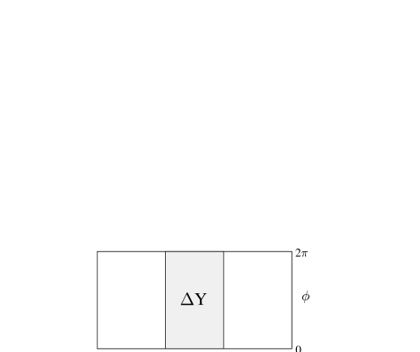
Figure 1: The acceptance region $\Delta Y$ in the plane of rapidity $y$ and azimuthal angle $\phi$. The window $\Delta Y$ is centered around $y=0$ here.

Since we cannot solve full QCD, but have to resort to perturbative treatment, we must carefully specify which collisions are to be considered perturbative, i.e. hard enough. We define the perturbative collisions to be those with a large enough amount ($\gg\Lambda_{\rm QCD}$) of transverse momentum produced, regardless of where the partons go in rapidity. For the different final state kinematics, this implies

$$2\rightarrow 2: p_{T1}+p_{T2}\geq 2p_{0}$$

$$2\rightarrow 3: \quad\quad\quad\quad p_{T1}+p_{T2}+p_{T3}\geq 2p_{0},\quad p_{0}\gg\Lambda_{\rm{QCD}}$$ (19)

where the parameter $p_{0}$, which restricts the computation below, is a fixed external parameter which does not depend on $\Delta Y$. For $2\rightarrow 2$ processes, appearing both in LO and in NLO, where the scattered partons are back-to-back in the transverse plane, the condition above means that individual minijets, inside or outside $\Delta Y$ always have $p_{T}\geq p_{0}$. For the $2\rightarrow 3$ processes, which appear only in NLO, a single parton may have also less than $p_{0}$ transverse momentum as long as the total transverse momentum released in the partonic process exceeds $2p_{0}$. This feature, which is also the main difference to the formulation of the same problem in Ref. [33], will have interesting implications later on. We will investigate the dependence of the results on $p_{0}$ and whether the NLO results remain stable relative to LO as $p_{0}$ is taken into the few-GeV realm. To estimate the transverse energy produced in $AA$ collisions at RHIC and LHC, additional phenomenology (see e.g [22]) needs to be introduced. This phenomenology will be separately discussed in Sec. 4.

The infrared safe measurement functions $S_{2}$ and $S_{3}$ [30] can now be written down by combining the definitions of perturbativeness of the collisions and the definition of $E_{T}$ in $\Delta Y$. For $2\rightarrow 2$ scatterings, we define

$$S_{2}(p_{1}^{\mu},p_{2}^{\mu})=\Theta(p_{T1}+p_{T2}\geq 2p_{0})\delta(E_{T}-[\epsilon(y_{1})p_{T1}+\epsilon(y_{2})p_{T2}])$$ (20)

and for $2\rightarrow 3$ scatterings correspondingly

$$S_{3}(p_{1}^{\mu},p_{2}^{\mu},p_{3}^{\mu})=\Theta(p_{T1}+p_{T2}+p_{T3}\geq 2p_{0})\delta(E_{T}-[\epsilon(y_{1})p_{T1}+\epsilon(y_{2})p_{T2}+\epsilon(y_{3})p_{T3}]).$$ (21)

where $\Theta$ is a step function.

It is easy to verify that these measurement functions indeed fulfill the requirements (7) and (8) for infrared safety. This is also intuitively clear, as the total $E_{T}$ is not sensitive to whether it is carried by one parton or two collinear partons, or by two partons of which one is at the soft limit.

The measurement functions above define the semi-inclusive $E_{T}$ distribution of minijets in $\Delta Y$ in $pp$ collisions, introduced in LO in [13]. Extending this now to NLO gives

$$\frac{d\sigma}{dE_{T}}\bigg{|}_{p_{0},\Delta Y} = \frac{d\sigma}{dE_{T}}\bigg{|}_{p_{0},\Delta Y}^{2\rightarrow 2}+\frac{d\sigma}{dE_{T}}\bigg{|}_{p_{0},\Delta Y}^{2\rightarrow 3}$$

$$= \int d[PS]_{2}\frac{d\sigma^{2\rightarrow 2}}{d[PS]_{2}}S_{2}(p_{1}^{\mu},p_{2}^{\mu})+\int d[PS]_{3}\frac{d\sigma^{2\rightarrow 3}}{d[PS]_{3}}S_{3}(p_{1}^{\mu},p_{2}^{\mu},p_{3}^{\mu}),$$

with the notation as in Eq. (2).

The minijet $E_{T}$ distribution above is normalized to the integrated cross section $\sigma_{\rm jet}(\sqrt{s},p_{0})$, as explained in [13]. As a side remark, we note that although we do not explicitly consider the computation of $\sigma_{\rm jet}$ here, it is an infrared safe quantity to compute, i.e. the extension of its definition to NLO can be done. The main interest now, as already emphasized, is to study the behaviour of the first moment of the $E_{T}$ distribution (LABEL:dET) as a function of the parameter $p_{0}$ which defines the extent of our perturbative calculation. Integrating the delta functions away in Eq. (LABEL:dET) we get

$$\sigma_{\rm QCD}\langle E_{T}\rangle_{\Delta Y,p_{0}}\equiv\int_{0}^{\sqrt{s}}dE_{T}\,E_{T}\frac{d\sigma}{dE_{T}}\bigg{|}_{p_{0},\Delta Y}=\sigma\langle E_{T}\rangle_{\Delta Y,p_{0}}^{2\rightarrow 2}+\sigma\langle E_{T}\rangle_{\Delta Y,p_{0}}^{2\rightarrow 3},$$ (23)

where

$$\sigma\langle E_{T}\rangle_{\Delta Y,p_{0}}^{2\rightarrow 2} = \int d[PS]_{2}\frac{d\sigma^{2\rightarrow 2}}{d[PS]_{2}}\tilde{S}_{2}(p_{1}^{\mu},p_{2}^{\mu})$$ (24)

$$\sigma\langle E_{T}\rangle_{\Delta Y,p_{0}}^{2\rightarrow 3} = \int d[PS]_{3}\frac{d\sigma^{2\rightarrow 3}}{d[PS]_{3}}\tilde{S}_{3}(p_{1}^{\mu},p_{2}^{\mu},p_{3}^{\mu}).$$ (25)

The measurement functions for the first $E_{T}$-moment above are denoted by

$$\tilde{S}_{2}(p_{1}^{\mu},p_{2}^{\mu}) = \bigg{[}\epsilon(y_{1})+\epsilon(y_{2})\bigg{]}p_{T2}\Theta(p_{T2}\geq p_{0})$$ (26)

$$\tilde{S}_{3}(p_{1}^{\mu},p_{2}^{\mu},p_{3}^{\mu}) = \bigg{[}\epsilon(y_{1})p_{T1}+\epsilon(y_{2})p_{T2}+\epsilon(y_{3})p_{T3}\bigg{]}\Theta(p_{T1}+p_{T2}+p_{T3}\geq 2p_{0}),$$ (27)

where $p_{T1}=p_{T2}$ in the former term and $p_{T1}=|{\bf p}_{T2}+{\bf p}_{T3}|$ in the latter one. Naturally, also $\tilde{S}_{2}$ and $\tilde{S}_{3}$ fulfill the criteria (7) and (8), which ensures that $\sigma\langle E_{T}\rangle_{\Delta Y,p_{0}}$ is a well-defined infrared safe quantity to compute. From the general form of the equations above, we notice that, by replacing the measurement functions $S_{2}$ and $S_{3}$ in Eq. 2 by $\tilde{S}_{2}$ and $\tilde{S}_{3}$ defined above, we can exactly follow the formulation and solution of the problem as given in ref. [30] and summarized in the previous section.

Finally, apart from the measurement functions themselves but related to the problem being infrared safely defined, the renormalization scale $\mu_{R}$ in the strong coupling $\alpha_{s}(\mu_{R})$ and the factorization scale $\mu_{F}$ in the parton distributions $f_{i}(x,\mu_{F})$ have to be chosen in such a way that the scales for the $2\rightarrow 3$ terms reduce to those for the terms with $2\rightarrow 2$ kinematics in the soft and collinear limits.

3 Numerical Evaluation

The formulation of the minijet $E_{T}$ production thus exists. To study its implications and to estimate its usefulness a numerical study has to be carried out next.

Due to the simple structure of the two-particle phase space, one can analytically describe the kinematically allowed region with the cuts imposed by $\Delta Y$. The part consisting of two-particle final states is therefore easily evaluated with a high precision by using the available integration routines of the fortran NAG-library [36].

The seven-dimensional phase space integral over the three-particle phase space reduces to a six-dimensional one after the symmetry of the measurement function $S_{3}$ under the azimuthal angle $\phi_{2}$ is taken into account. In principle, these six-dimensional integrals could be treated similarly as the three-dimensional ones over the two-particle phase space, but due to the additional kinematical cuts introduced by the subtraction terms (the additional step functions in Eq. (12)) this does not work out in practice. Rather one is forced to use fairly crude and quite time-consuming Monte Carlo integration. We have used another NAG subroutine to take care of these terms. Fortunately, the major part of the cross sections comes from the Born level terms plus the finite parts of the subtraction terms having $2\rightarrow 2$ kinematics. The finite terms with $2\rightarrow 3$ kinematics are smaller and therefore their contribution to the total relative numerical error of the results is estimated to be rather small, below four per cent in any case.

In the numerical evaluation of the integrands with $2\rightarrow 3$ we are able to use certain subroutines of the jet-program of Ellis, Kunszt and Soper [37]. Also the partonic book-keeping is taken care of by adopting the method and the permutation tables of different subprocesses used in the program of EKS. The number of flavors is fixed to be $N_{f}=4$, and calculations were performed using two different sets of parton distribution functions (PDF): GRV94 [38] and a more recent set CTEQ5 [39]. For $\Lambda_{\rm QCD}$ we take the value as quoted in the PDF set used.

Before the numerical evaluation, also the renormalization and factorization scales have to be fixed. In principle, the dependence of the results on $\mu_{R}$ and $\mu_{F}$ should be studied independently. In practise, however, the Monte Carlo integrals being tedious to solve numerically, we follow the common practise and choose these to be equal, $\mu_{R}=\mu_{F}\equiv\mu$, and study the dependence of the results on $\mu$ only. Regarding the scale itself, the most physical choice should reflect the perturbativeness of the collision, therefore we set $\mu$ proportional to the total transverse momentum produced in the hard process, regardless whether the partons are in $\Delta Y$ or not,

$$2\rightarrow 2:\quad\mu = N_{\mu}\times\frac{1}{2}(p_{T1}+p_{T2})=N_{\mu}\times p_{T}$$ (28)

$$2\rightarrow 3:\quad\mu = N_{\mu}\times\frac{1}{2}(p_{T1}+p_{T2}+p_{T3}),$$

where $N_{\mu}$ is a constant of the order of unity. This choice is infrared safe in the sense of Eqs. (7)-(8), as is required for the exact cancellation of the divergent terms. We also note that with this scale choice one is able to include the new kinematical region, where two partons fall outside $\Delta Y$ and one with small momentum ($p_{T}<p_{0}$) falls inside, contributing thus to the region $E_{T}<p_{0}$ not present in the computation of the perturbative $2\rightarrow 2$ processes.

As there is some freedom in choosing the scale, other possibilities can also be thought of. For example in Ref. [33] the total $E_{T}$ entering $\Delta Y$ was considered. This, we think, leads to an ambiguity already at the $2\rightarrow 2$ level, as almost identical hard subprocesses are given very different scales depending whether both of the partons fly into $\Delta Y$ or not. This issue is also clearly connected with the definition of the perturbativity of the partonic processes, i.e. which collisions are to be included in the computation and which excluded. For high-$p_{T}$ jets, of course, $\mu\sim p_{T}^{\rm{jet}}$ is the most natural scale choice, but in our case we would like to emphasize the semi-inclusive nature of the problem, and also that the minijet $E_{T}$ distribution is, unfortunately, not a direct observable, especially not in $AA$ collisions.

4 Results

4.1 Dependence on $p_{0}$ and on the PDF set

The main goal, for the reason of the importance of the semihard region in initial $E_{T}$ production in $AA$ collisions, is now to study the behaviour of $\sigma\langle E_{T}\rangle$ as the parameter $p_{0}$ controlling the perturbativity is taken from large scales into the few-GeV domain. On the basis of high-$p_{T}$ inclusive jet computations [28, 29, 40] one may well expect fairly large NLO contributions: at scales of few tens of GeV, say, NLO improved results may well be larger by a factor of two as compared to LO ones. This largeness in the absolute magnitude of the correction terms does not imply that the perturbation series would be in a stall well out of the region of convergence, but rather is a signal of the possibility of some new element becoming manifest only at such high order. For the case of observable jets, the new element is the dependence of the NLO cross sections on the jet cone $R$. Another well-known example of precisely such a case is the Drell-Yan dilepton production where the NLO corrections bring in QCD as a new element [41]. In this sense, the question of the convergence of the perturbation series is moved to the behaviour of the next-to-next-to-leading order terms.

In our case the new element the NLO definition of the problem introduces, is the appearance of a new kinematical region: for $2\rightarrow 2$ processes, the $E_{T}$ distribution is empty at scales $E_{T}<p_{0}$ but not anymore so in the $2\rightarrow 3$ case. The crucial question therefore concerns the behaviour of the results as $p_{0}$ is decreased from, say, 10 GeV down to to 1…2 GeV. If the NLO result is of a similar magnitude as at 10 GeV, as will be shown to be the case, the conclusion is that the NLO result is stable and pQCD can be appealed to at such small scales. Another interesting point, already studied in [32], is the dependence of $\sigma\langle E_{T}\rangle$ on the choice for the renormalization and factorization scale, and whether this behaviour substantially deviates from that in LO.

To study the stability in the sense described above we define two $K$-factors:

$$K^{\prime}=\frac{\rm{NLO}}{\rm{LO^{\prime}}},\quad\quad K=\frac{\rm{NLO}}{\rm{LO}},$$ (29)

where LO^′ is the first term of the NLO expansion, i.e. it is the Born term evaluated with 2-loop $\alpha_{s}$ and NLO parton distribution functions. Unprimed LO stands for leading order result evaluated with 1-loop $\alpha_{s}$ and LO parton distribution functions, this being the “truly” leading order result. These two $K$-factors tell different tales: The unprimed $K$ is the one commonly introduced in the LO computations to bring the elements of NLO in. The $K^{\prime}$ on the other hand measures roughly the difference between two subsequent terms in the perturbation series, and possibly carries somewhat more information about the actual convergence of the perturbation series, since in $K^{\prime}$ the same parton distributions appear both in the nominator and denominator. Which one is more relevant, is somewhat of a matter of taste, though, and this is why both $K$-factors are discussed.

Figure 2: (a) The first moment $\sigma\langle E_{T}\rangle$ of the minijet $E_{T}$ distribution as a function of the minimum transverse momentum scale $p_{0}$. Three curves for both RHIC, $\sqrt{s}=200$ GeV, and LHC, $\sqrt{s}=5500$ GeV, are shown: the solid lines are the full NLO results computed with the GRV94-HO parton distributions, the dashed lines are the LO results evaluated with 2-loop $\alpha_{s}$ and NLO parton distributions, and the dotted lines in between are the truly LO results evaluated with 1-loop $\alpha_{s}$ and GRV94-LO parton distributions. The scale choice for all points in this figure is $N_{\mu}=1$ in Eq. (3). (b) The same but computed with the CTEQ5M and CTEQ5L parton distributions. Labelling of the curves is same as in panel a.

In Fig. 2a the results for $\sigma\langle E_{T}\rangle$ computed with GRV94 parton distribution functions are shown as a function of the parameter $p_{0}$. The solid curves are the NLO results, the dotted and dashed ones show the LO results computed in the two different ways described above. In Fig. 2b we repeat the calculation by using the CTEQ5 parton distribution functions. The corresponding $K$-factors ($K$ and $K^{\prime}$) are collected in Table 2 for some values of $p_{0}$ from both figures. The immediate observation from the figures and the table is that the full NLO results deviate very systematically from the LO ones: Both $K$ and $K^{\prime}$ increase as $p_{0}\rightarrow 1$ GeV, but the factor $K$ appears to increase less than the factor $K^{\prime}$. The steady increase in $K^{\prime}$ can be understood as a signal of the nearby borderline of pQCD. In a more practical sense the differences between LO and LO^′ arise at RHIC energies from the differences in $\alpha_{s}$ and $\Lambda_{\rm{QCD}}$ and at LHC energies, in addition to the previous, from the difference between the LO and NLO parton distributions.

Based on the more stable behaviour of $K$, it may well be argued that if one trusts the perturbative computation at 10 GeV scale, one can equally well count on it also at 2 or 3 GeV scales. Another observation is that the $K$-factors do depend on the PDF sets chosen.

$p_{0}$	$K_{RHIC}^{\prime GRV(CTEQ5)}$	$K_{RHIC}^{GRV(CTEQ5)}$	$K_{LHC}^{\prime GRV(CTEQ5)}$	$K_{LHC}^{GRV(CTEQ5)}$
1	4.8 (5.9)	2.2 (3.4)	-	-
2	3.6 (4.2)	2.2 (3.3)	4.2 (4.9)	1.5 (2.1)
4	3.0 (3.2)	2.1 (3.0)	3.4 (3.9)	1.5 (2.2)
6	2.7 (3.0)	2.0 (2.9)	3.2 (3.5)	1.6 (2.2)
8	2.4 (2.6)	1.9 (2.7)	3.0 (3.3)	1.6 (2.2)
10	2.3 (2.5)	1.8 (2.7)	2.9 (3.1)	1.6 (2.2)

Table 2: Values of the two $K$-factors defined in the text for different values of $p_{0}$. The numbers are shown for both RHIC and LHC energies and for two different PDF-sets, the GRV94 and CTEQ5.

It should be emphasized once more, that here $p_{0}$ is to be strictly regarded as an external parameter, on which the dependence of the results is studied. To form the initial $E_{T}$ in $AA$ at RHIC and at the LHC, one has to decide upon at which value of $p_{0}$ the $\sigma\langle E_{T}\rangle$ should be taken. The expectation is that $p_{0}\sim 1\dots 2$ GeV, possibly depending on $\sqrt{s}$ and $A$ [22], but precise estimation of this value is beyond the perturbative approach in the sense that it requires introduction of further phenomenology or knowledge of non-perturbative physics involved. Regardless of the actual mechanism to determine the suitable value of $p_{0}$ the basic question of applicability of pQCD in the few-GeV domain remains, and it is precisely this question that is currently being answered.

4.2 Dependence on the scale choice

The dependence of $\sigma\langle E_{T}\rangle$ on the renormalization/factorization scale $\mu$, chosen according to in Eq. (3), has essentially been presented in Ref. [32] but for completeness let us discuss this a bit further here. In Fig. 3, we plot $\sigma\langle E_{T}\rangle$ at a fixed value $p_{0}=2$ GeV as a function of the $N_{\mu}$ in Eq. (3). The results in Fig. 2(a) for this $p_{0}$ are found at $N_{\mu}=1$ in the figure.

At RHIC the results depend somewhat on the chosen scale. This behaviour is as what could be expected on the basis of the studies of cross sections of observable jets [29, 40], where it is more difficult to find a plateau as a function of $\mu/p_{T}$ towards smaller jet momenta. At the LHC $\sigma\langle E_{T}\rangle$ exhibits a clear plateau around $N_{\mu}\sim 1$. Similar behaviour is observed already in both leading order curves, due to cancellation between the rise of gluon distributions and the decrease of $\alpha_{s}$ with an increasing scale. Therefore the plateau cannot be attributed to a fast convergence of the perturbation series but the NLO results depend equally strongly (RHIC) or weakly (LHC) on the scale choice as the LO results do. Another consequence of this is that the $K$-factor is close to constant near $N_{\mu}\sim 1$.

Figure 3: The first moment $\sigma\langle E_{T}\rangle$ as a function of $N_{\mu}=\mu/\sum_{i}(p_{Ti})$ (see Eq. (3)) at a fixed value of $p_{0}=2$ GeV. The labelling of the curves is same as in Figs. 2, and the GRV94 parton distributions have been used.

4.3 A new kinematical region

As noted already in our earlier work [32], the NLO computation allows for a new kinematical region to be included. The existence of such a new contribution arises in the following way: in LO and in the loop-corrected NLO terms, where only $2\rightarrow 2$ processes are considered, the two final state partons are produced back-to-back with equal transverse momenta. The smallest amount of $E_{T}$ entering the acceptance region $\Delta Y$ is therefore equal to $p_{0}$, and consequently the minijet $E_{T}$-distribution is completely empty below $E_{T}=p_{0}$. In NLO, however, the $2\rightarrow 3$ scatterings are included and the situation where one of the three partons has transverse momentum smaller than $p_{0}$ but the other two have larger momenta, as required by the condition $p_{T1}+p_{T2}+p_{T3}\geq 2p_{0}$ and momentum conservation, may arise. Now, the two partons having transverse momenta larger than $p_{0}$ may fall outside the acceptance window and only the third one with $p_{T}$ equal to a fraction of $p_{0}$ enters $\Delta Y$, thus adding a contribution from the domain $E_{T}\leq p_{0}$ into the $E_{T}$-distribution.

To identify the contribution from the new domain at $E_{T}<p_{0}$ from the results shown in Figs. 2, we compute $\sigma\langle E_{T}\rangle$ by performing the integration in Eq. (23) from $E_{T}=p_{0}$ to $\sqrt{s}$ instead of integrating all the way from 0. To the measurement function (27) this adds a term $\Theta(E_{T}\geq p_{0})$. This is actually close to the approach of Ref. [33] (but still not the same, as our $p_{0}$ is a constant independent of $\Delta Y$), where the new kinematic region is not included. The obtained results are shown in Fig 4, and the value of the resulting $K^{\prime}$-factor is comparable with the ones obtained in [33].

Figure 4: (a) The quantity $\sigma\langle E_{T}\rangle$ as a function of $p_{0}$, computed as in Fig. 2(b) but with an additional cut $\theta(E_{T}\geq E_{0}=p_{0})$). Labelling of the curves is the same as in Figs. 2, and CTEQ5 partons distributions are used. Note that the LO curves (dotted and dashed) are identical with those in Fig. 2(b).

Comparing this figure with Fig. 2b, one observes that the $K$-factors come down by a factor of two, hence enhancing the indications of the validity of the perturbative treatment. At the LHC energy, and at RHIC for $p_{0}\sim 1$ GeV, the NLO result shows practically no deviation from the truly LO one. Also, by comparison of the two figures, the slight growth of the $K$ factors, especially relative to LO^′, can now be attributed to the inclusion of the new kinematical region at $E_{T}<p_{0}$. The conclusion thus is that a new kinematical domain at $E_{T}\leq p_{0}$ not only exists, but it is also an important new feature in the extension of the problem to NLO. This also hints that if a convergence of the perturbation series is looked for in the semihard region, at least a NNLO computation should be studied.

It is also interesting to note that inclusion of the new kinematical domain brings the perturbative approach towards the studies of the classical field configurations [42, 43, 44, 45], where the dominant contribution is obtained from the process of two valence quarks exchanging a gluon and emitting a gluon. All such three-particle processes, and most importantly the purely gluonic ones, are now rigorously included in our computation, supplemented of course with the criterion for perturbativity, i.e. that in our approach the partons which scatter forward and backward outside $\Delta Y$, are required to carry large enough $p_{T}$.

4.4 Dependence on $\Delta Y$

So far all the results presented have been evaluated for the central rapidity unit, and it would certainly be desirable to know how the results change as the rapidity interval $\Delta Y$ (centered around $y=0$) is varied. This is shown in Fig. 5, where $\sigma\langle E_{T}\rangle$ is plotted as a function of $\Delta Y$, keeping $p_{0}$ at a fixed value of 2 GeV. The results are seen to be nearly linear in $\Delta Y$ around $\Delta Y=1$.

Figure 5: The quantity $\sigma\langle E_{T}\rangle$ as a function of the rapidity acceptance window $\Delta Y$ with a fixed value of $p_{0}=2$ GeV. The three lower curves are for RHIC and the three topmost curves for the LHC. As before, the solid curves stand for the NLO results, and the dotted and dashed ones for the LO results.

In fact this is an important result as it increases confidence in computing the initial conditions from pQCD [22] in the following way: The average initial energy densities in the central spatial region, $z\sim 0$, can be estimated through the Bjorken formula [3]

$$\epsilon_{i}=\frac{E_{T}^{AA}({\bf{b}}=0,\sqrt{s},p_{0},\Delta Y)}{\pi R_{A}^{2}\tau_{0}\Delta Y},$$ (30)

where the initial time $\tau_{0}=1/p_{0}$ and the spatial rapidity interval in the longitudinal volume element in the denominator has been taken to be $\Delta Y$. As seen in Fig. 5, the initial transverse energy $\bar{E}_{T}^{AA}=T_{AA}\sigma\langle E_{T}\rangle$ behaves in LO essentially linearly in $\Delta Y$ near the central rapidities and the $\Delta Y$ dependence is thus cancelled out in the initial energy density of Eq. (30). Based on the NLO computation of the cross sections of observable jets [29], it could be expected that $\Delta Y$ plays the role of the jet cone $R$ and the NLO results would therefore exhibit a different behaviour ($\sim R^{2}$ at large $R$) in $\Delta Y$ than the LO results. From the point of view of the local energy densities obtained through Eq. (30) this would be disastrous as $\epsilon_{i}$ would badly depend on the $\Delta Y$ chosen. As clearly seen in the figure, this is now not the case but the NLO results behave nicely in a similar way as the LO results do. This implies that the initial energy densities are not sensitive to the detailed size of the rapidity interval. One should also pay attention to the difference between the calculation of $E_{T}$ of ordinary jets and the calculation of $E_{T}$ in $\Delta Y$ from minijets considered in here: the jet calculation introduces an additional dependence on a resolution parameter, the jet cone radius $R$, which is simply absent in our considerations.

4.5 Nuclear effects

It is a well known fact that the distribution of partons in a free proton are different from those of a proton bound to a nucleus, $f_{i/A}(x,\mu^{2})=R_{i}^{A}(x,\mu^{2})f_{i}(x,\mu^{2})$ with $R_{i}^{A}\neq 1$. Regarding the behaviour of $\sigma\langle E_{T}\rangle$, the last point of study here is the effect of an inclusion of nuclear effects $R_{i}^{A}(x,Q^{2})$ in the parton distributions. This is done by using the EKS98 parametrization [20] which is based on a DGLAP analysis of the nuclear parton distributions, with constraints from the existing data from deep inelastic $lA$ scattering and Drell-Yan production in $pA$ and also from momentum and baryon number conservation. There are definite sources of uncertainties we implicitly accept when using EKS98: First, the nuclear modifications have been shown to be independent of the PDF set chosen within a level of a few per cent error [20]. Second, the EKS98 is based on a LO DGLAP evolution equations only but we apply it to the NLO PDFs as well. Finally, the nuclear gluon distributions themselves are still largely unknown at $x\raise 1.29167pt\hbox{$<$\kern-7.5pt\raise-4.73611pt\hbox{$\sim$}}0.01$, a region which is important for the few-GeV minijets at the LHC. For RHIC, the situation is better since for $0.01\raise 1.29167pt\hbox{$<$\kern-7.5pt\raise-4.73611pt\hbox{$\sim$}}x\raise 1.29167pt\hbox{$<$\kern-7.5pt\raise-4.73611pt\hbox{$\sim$}}0.2$ some constraints can be obtained from the $Q^{2}$ dependence of the ratio of the structure functions $F_{2}^{\rm Sn}/F_{2}^{\rm C}$ measured by the New Muon collaboration in deeply inelastic lepton-nucleus scatterings [46].

Figure 6: (a) The $\sigma\langle E_{T}\rangle$ as in fig. 2(a) but also nuclear shadowing has been taken into account via EKS98 parametrization [20]. The computation has been carried our for a nucleus $A$=208 for both energies. (b) Comparison of the $\sigma\langle E_{T}\rangle$ with nuclear shadowing (solid and dotted lines) and without shadowing (dot-dashed and dashed lines). The curves are shown for RHIC (lower four curves) and LHC (upper four curves). Of the four curves the upper pair is the full NLO result and the lower pair is the truly LO result.

The validity region of the EKS98 does not quite extend down to $\mu=1$ GeV, so we limit the study of nuclear effects in the NLO study of $\sigma\langle E_{T}\rangle$ to $p_{0}$ between 2 and 10 GeV. The results can be found in Fig. 6 below. In the first panel, the nuclear effects are included in all curves, the labelling of which is the same as in previous figures. The corresponding $K$-factors are collected in Table 3. Comparison of the numbers with those in parentheses in Table 2 indicates that the effects of the nuclear modifications to the $K$-factors can be neglected at RHIC, whereas for the LHC there is a slight increase towards the region $p_{0}\sim 2$ GeV. The reason for this can be understood based on the second panel, where a comparison between the results with and without the nuclear effects is shown. For RHIC near $p_{0}\sim 2$ GeV, one is in the region where the nuclear effects of gluons stay very small as the cross-over region between shadowing ($R_{g}^{A}<1$) and anti-shadowing ($R_{g}^{A}<1$) is probed (For $2\rightarrow 2$, typically $x\sim 2p_{0}/\sqrt{s}$). Towards $p_{0}\sim 1$ GeV one would move into the shadowing region but the nuclear effects remain quite small in any case. At the LHC, the shadowing effects are larger, about 30% for the LO and 20% for the NLO results. The difference is due to the new kinematical region included: in the region $E_{T}<p_{0}$, where typically $y_{1}>0.5$ and $y_{2}<0.5$ and $p_{3}$ is small, the values of $x_{1}$ and $x_{2}$ are slightly larger than the typical $x_{1,2}$ in LO. The net loss in the gluonic luminosity due to shadowing is then altered less than in LO.

$p_{0}$	$K_{RHIC}^{\prime}$	$K_{RHIC}$	$K_{LHC}^{\prime}$	$K_{LHC}$
2	4.2	3.3	5.5	2.5
4	3.2	3.0	4.2	2.3
6	2.9	3.0	3.7	2.3
8	2.7	2.7	3.3	2.2
10	2.6	2.7	3.1	2.2

Table 3: Values of the two $K$-factors defined in Eq. (29) for different values of $p_{0}$. The parton distribution functions are those of the CTEQ5-set and the nuclear shadowing is included through the EKS98 parametrization.

5 From $p_{0}$ to $p_{\mbox{\scriptsize sat}}$?

As described in the introduction, the goal of the present paper is to study the main uncertainties in the collinearly factorized minijet formalism to the initial production of transverse energy in ultrarelativistic nuclear collisions. Now that we have control over the NLO corrections in the quantity $\sigma\langle E_{T}\rangle$ and have also verified that they do not present significantly divergent results at scales of few GeV, we may, as an application, turn to a determination of the actual value of the scale $p_{0}$. As emphasized already in the introduction, this requires additional phenomenology. Here we will work in the framework of Ref. [22].

At certain scale $p_{0}=p_{\mbox{\scriptsize sat}}(\sqrt{s},A)$ the system of gluons produced into the central unit of rapidity will reach a density such that the effective total area of these gluons $N_{AA}(\sqrt{s},p_{\rm sat})\times\pi/p_{\mbox{\scriptsize sat}}^{2}$ will be equal to the transverse area $\pi R_{A}^{2}$ in central collisions. Performing the computation at a scale $p_{0}=p_{\mbox{\scriptsize sat}}$ will effectively estimate the contributions of all scales in the sense that gluons with $p_{T}\ll p_{\mbox{\scriptsize sat}}$ would contribute negligibly to the total $E_{T}$. Hence, if $p_{\mbox{\scriptsize sat}}$ falls into the perturbatively computable region, above $\sim$ 1 GeV, the initial energy densities can be obtained from the perturbative computation alone. For nuclei with $A\sim 200$ and collision energies of the order of 100 GeV this has been shown to be the case [22].

To demonstrate the effects of the NLO terms and shadowing corrections, a determination of the scale $p_{{\mbox{\scriptsize sat}}}$ is illustrated in the upper panel of Fig. 7, showing the number of minijets in a central $AA$ collision of $A=208$, $N_{AA}(b=0,p_{0},\sqrt{s},\Delta Y)=T_{AA}(0)\times 2\sigma_{\rm jet}(p_{0},\sqrt{s},\Delta Y)$ [47] in the rapidity acceptance region $\Delta Y$. There is, however, a theoretical caveat in computing the number of minijets, or rather $2\sigma_{\rm jet}(p_{0},\Delta Y)=\sigma\langle n\rangle$, the first moment of the number distribution of minijets in $\Delta Y$ to NLO. A strictly infrared safe definition of a measurement function for $\sigma\langle n\rangle$ requires an introduction of an additional resolution scale, such as a screening mass, which defines when two nearly collinear partons within $\Delta Y$ are to be counted as one and when as two. A detailed formulation of this is beyond the scope of the present paper, so let us simply simulate the NLO terms by taking the $K$-factors computed for $\sigma\langle E_{T}\rangle$ and multiply the LO results for $N_{AA}$ by them. The value of $p_{0}$ can then be determined by the intersection points of $N_{AA}(p_{0})$ with the saturation curve $N_{AA}(p_{0})=p_{0}^{2}R_{A}^{2}$. In the lower panel we show the results for the initial transverse energy $E_{T}^{AA}=T_{AA}\sigma\langle E_{T}\rangle$ with and without shadowing. The initial $E_{T}$ can then be read off from the different curves at each saturation scale $p_{0}=p_{\rm sat}$.

Figure 7: Upper panel shows the determination of the scale $p_{{\mbox{\scriptsize sat}}}$. The saturation curve, $N_{AA}(p_{0})=p_{0}^{2}R_{A}^{2}$ is shown by the dashed line labeled ‘saturation’. 2 sets of four curves are shown. The upper four curves are for LHC energies and the lower ones are for RHIC. The solid lines are the LO results with GRV94 parton distributions multiplied by $K(p_{0})$ from the $\sigma\langle E_{T}\rangle$ analysis, and the dotted ones are the LO results with GRV94 without the $K$-factor. The dashed lines stand for the LO results with CTEQ5 and the dot-dashed lines for the LO results with CTEQ5+EKS98, multiplied with respective $K(p_{0})$ from the $\sigma\langle E_{T}\rangle$ calculation with the same PDFs. The value of $p_{{\mbox{\scriptsize sat}}}$ can be read off in the intersection points of the ‘saturation’-curve with the other curves. The corresponding values of $E_{T}(p_{{\mbox{\scriptsize sat}}})$ can be read off from the curves at the lower panel.

It is interesting to note, as pointed out already in [22], that at the saturation scale $p_{0}=p_{\rm sat}$ the computed $E_{T}^{AA}/N_{AA}$ is very close to $E/N=\epsilon_{i}/n_{i}=2.7T_{i}$ of an ideal gas of massless bosons, where the temperature $T$ is obtained from $\epsilon_{i}=aT^{4}$ with $a=16\pi^{2}/30$. From the point of view of energy per particle, a very rapid thermalization seems thus plausible. Recent studies [11, 12, 48] indicate that this may indeed be the case, although early thermalization is still a subject of debate [49]. In any case, it is worth emphasizing that in our approach saturation and apparent thermalisation take place simultaneously.

In fact, the early thermalisation could be used to get rid of the worry that the saturation approach involves a non-infrared safe quantity: one could first compute the thermalised initial parton number $N_{i}(p_{0})$ as a function of $p_{0}$ from the infrared safe initial $E_{T}$ as $E_{T}^{AA}(p_{0})\rightarrow\epsilon_{i}(p_{0})\rightarrow T_{i}(p_{0})\rightarrow s_{i}(p_{0})\rightarrow N_{i}(p_{0})$, and then use the obtained thermal $N_{i}(p_{0})$ in the saturation criterion to determine $p_{\rm sat}$.

If the system is thermal at $p_{\rm sat}$ and if its further evolution is isentropic, the initial number of particles reflects the final multiplicity per unit rapidity quite closely, $N_{f}\approx 0.9N_{AA}(p_{\rm sat},\sqrt{s})$ [22]. Figure 7 can therefore be directly used to estimate the effects from the NLO contributions, parton distribution functions and shadowing to $N_{f}$. If the NLO corrections are taken into account via the $K$-factor, then from the saturation criterion $N_{AA}=p_{{\mbox{\scriptsize sat}}}^{2}R_{A}^{2}$ it follows, assuming that $N_{AA}\sim K/p_{{\mbox{\scriptsize sat}}}^{n}$, that $N_{AA}\sim K^{2/(n+2)}$. Furthermore taking $E_{T}\sim p_{{\mbox{\scriptsize sat}}}N_{AA}$ one finds that $E_{T}\sim K^{3/(n+2)}$. From the Fig. 7 we see that $n=3.0\dots 3.3$ at RHIC and $n=2.4\dots 2.7$ at LHC, depending whether shadowing is included or not. Let us take, say, $K\approx 2$ at RHIC and $K\approx 1.5$ at LHC. Then, using the smallest values for $n$ quoted above, one finds that at RHIC the increase with respect to the LO results in $N$ and $E_{T}$ is 30% and 50% respectively. At LHC the increase is 20% $N$ and 40% in $E_{T}$. This also demonstrates the importance of the inclusion of the NLO contributions

It is more difficult to give the theoretical uncertainty in the saturation criterion itself, due to the possible nonperturbative elements involved. The data coming now for the charged particle multiplicities from RHIC can in principle be used to constrain the remaining uncertainty in the saturation criterion. Once the scale $p_{0}=p_{\rm sat}$ is nailed down for one collision energy, predictions of the final state $E_{T}$ within the hydrodynamical approach can be computed with the initial energy densities obtainable based on the infrared safe NLO computation of $E_{T}^{AA}$. As mentioned in the introduction, a large decrease in $E_{T}$ is expected due to the work done by pressure. So far only longitudinally expanding QGP has been studied with minijet initial conditions [22], the results from a transversally expanding hydrodynamic system will be reported soon [50].

6 Conclusions

We have presented in detail the theoretical basis, implementation and numerical results of a rigorous perturbative QCD calculation of the amount of transverse energy produced from minijets in $AA$ or $pp$ collisions into a rapidity acceptance region. The formulation is based on collinear factorization. In particular, the quantity $\sigma\langle E_{T}\rangle$, the first moment of the minijet $E_{T}$ distribution, is computed and analysed.

Theoretically, the key point is the formulation of an infrared safe measurement function which gives the minijet $E_{T}$ distribution in $\Delta Y$ and includes the definition of perturbative collisions. The singularities arising in the NLO terms are cancelled by applying the subtraction method [28, 30]. The dependence of the results on the parton distribution functions, on the scale choice, on the width of the acceptance window and on nuclear effects in parton distributions have been studied in detail. Also, as an application, we have considered a way to fix the minimum transverse momentum scale $p_{0}$ in the saturation model [22], and the uncertainties from this procedure to the initial conditions of the QGP in $AA$ collisions at RHIC and LHC and also to the charged particle multiplicities in the final state.

The analysis of the full NLO results leads us to conclude that the NLO corrections are large but well behaved in the sense that their relative magnitude as compared to the LO results is not diverging as subprocesses with smaller and smaller amount of transverse energy exchanged were taken into account. Furthermore, the contributions from two different regions $E_{T}\geq p_{0}$ and from $E_{T}\leq p_{0}$ were studied. The latter one contributes only in NLO, through configurations where one small-$p_{T}$ parton enters $\Delta Y$ and the other two partons with larger transverse momenta fall outside the acceptance window. When the contribution from the new domain $E_{T}\leq p_{0}$ is excluded, the NLO corrections are observed to reduce by roughly a factor of two, and the stability of the results against the LO to increase. If the new domain is included, the comparison of the full NLO results against the LO numbers is not strictly one-to-one, since the new kinematical region is not present in LO at all. A consistent comparison in this case can therefore only be performed between NNLO and NLO contributions, as then contributions from all values of $p_{T}$ would be present. Our conjecture is that in that case suppression of NNLO terms will be observed.

Another important and beforehand not at all obvious result is that the initially produced $E_{T}$ in $AA$ collisions depends, contrary to what one might expect based on the jet cone dependence of high-$p_{T}$ jets, practically linearly on the chosen rapidity window $\Delta Y$. This has the important consequence that the local energy density does not depend on $\Delta Y$, and a possible source of ambiguity in estimation of the initial energy densities for the QGP in high energy $AA$ collisions is removed.

Finally, in connection to other models, in particular to the McLerran-Venugopalan model for gluon production through classical fields [24], the inclusion of the new kinematical region in our computation should bring these two approaches closer to each other.

Acknowledgements. We thank V. Ruuskanen for discussions and K. Kajantie for discussions and for collaboration in the early stages of the project. We thank the Center of Scientific Computing (CSC, Finland) for providing computational resources and P. Raiskinmäki for guidance in parallelisation of our code. The financial support from the Academy of Finland as well as from the Waldemar von Frenckell foundation is gratefully acknowledged.

References

- [1] B. Back et al. [PHOBOS Collaboration], “Charged particle multiplicity near midrapidity in central Au+Au collisions at =56 and 130 AGeV”, hep-ex/0007036.
- [2] K. H. Ackermann et al. [STAR Collaboration], “Elliptic flow in Au+Au collisions at =130 GeV”, nucl-ex/0009011.
- [3] J. D. Bjorken, Phys. Rev. D27 (1983) 140.
-
[4]
H. von Gersdorff, L. McLerran, M. Kataja and P. V. Ruuskanen,
Phys. Rev. D34 (1986) 794;
M. Kataja, P. V. Ruuskanen, L. McLerran and H. von Gersdorff, Phys. Rev. D34 (1986) 2755. -
[5]
K. Geiger and B. Müller, Nucl. Phys. B369 (1992) 600;
K. Geiger, Phys. Rept. 258 (1995) 237. - [6] B. Zhang, Comput. Phys. Commun. 109 (1998) 193, [nucl-th/9709009].
- [7] S. A. Bass et al., Prog. Part. Nucl. Phys. 41 (1998) 225, [nucl-th/9803035].
- [8] S. A. Bass et al., Prog. Part. Nucl. Phys. 42 (1999) 313, [nucl-th/9810077].
- [9] S. A. Bass and A. Dumitru, Phys. Rev. C61 (2000) 064909, [nucl-th/0001033].
- [10] G. C. Nayak, A. Dumitru, L. McLerran and W. Greiner, “Equilibration of the gluon minijet plasma at RHIC and LHC”, hep-ph/0001202.
- [11] A. H. Mueller, Nucl. Phys. B572 (2000) 227, [hep-ph/9906322].
- [12] R. Baier, A. H. Mueller, D. Schiff and D. T. Son, “‘Bottom-up’ thermalization in heavy ion collisions”, hep-ph/0009237.
- [13] K.J. Eskola, K. Kajantie and J. Lindfors, Nucl. Phys. B323 (1989) 37.
- [14] X.-N. Wang, Phys. Rev. D43 (1991) 104.
- [15] X.-N. Wang and M. Gyulassy, Phys. Rev. D44 (1991) 3501.
- [16] H. Pi, Comput. Phys. Commun. 71 (1992) 173.
- [17] K. Kajantie, J. Landshoff and J. Lindfors, Phys. Rev. Lett. 59 (1987) 2527.
- [18] J.P. Blaizot and A.H. Mueller, Nucl. Phys. B289 (1987) 847.
- [19] J. C. Collins, D. E. Soper and G. Sterman, Nucl. Phys. B261 (1985) 104.
-
[20]
K. J. Eskola, V. J. Kolhinen and P. V. Ruuskanen,
Nucl. Phys. B535 (1998) 351, [hep-ph/9802350] ;
K. J. Eskola, V. J. Kolhinen and C. A. Salgado, Eur. Phys. J. C. (1999) 61, [hep-ph/9807297]. - [21] L. V. Gribov, E. M. Levin and M. G. Ryskin, Phys. Rept. 100 (1983) 1.
- [22] K. J. Eskola, K. Kajantie, P. V. Ruuskanen and K. Tuominen, Nucl. Phys. B570 (2000) 379 [hep-ph/9909456].
- [23] K. J. Eskola, K. Kajantie, and K. Tuominen, “Centrality dependence of multiplicities in ultrarelativistic nuclear collisions”, hep-ph/0009246, submitted to Phys. Lett. B.
- [24] L. McLerran and R. Venugopalan, Phys. Rev. D49 (1994) 2233, [hep-ph/9309289].
- [25] A. Krasnitz and R. Venugopalan, Nucl. Phys. B557 (1999) 237, [hep-ph/9809433].
- [26] A. Krasnitz and R. Venugopalan, “The initial gluon multiplicity in heavy ion collisions”, hep-ph/0007108.
- [27] A. Krasnitz and R. Venugopalan, Phys. Rev. Lett. 84 (2000) 4309, [hep-ph/9909203].
- [28] S. D. Ellis, Z. Kunszt and D. E. Soper, Phys. Rev. D40 (1989) 2188.
- [29] S. D. Ellis, Z. Kunszt and D. E. Soper, Phys. Rev. Lett. 64 (1990) 2121.
- [30] Z. Kunszt and D. E. Soper, Phys. Rev. D46 (1992) 192.
- [31] R. K. Ellis and J. C. Sexton, Nucl. Phys. B269 (1986) 445.
- [32] K. J. Eskola and K. Tuominen, Phys. Lett. B489 (2000) 329, [hep-ph/0002008].
- [33] A. Leonidov and D. Ostrovsky, Eur. Phys. J.C11 (1999) 495, [hep-ph/9811417].
- [34] Z. Kunszt, ETH-TH-96/05, lectures presented at TASI 95, Boulder, June 1995, hep-ph/9603235.
- [35] S. D. Ellis, Z. Kunszt and D. E. Soper, Phys. Rev. Lett. 69 (1992) 1496.
- [36] NAG Fortran Library, Mark 18.
- [37] S. D. Ellis, Z. Kunszt and D. E. Soper, JET version 3.4, 18 March 1997.
- [38] M. Glück, E. Reya and A. Vogt, Z. Phys. C67 (1995) 433.
- [39] H. L. Lai et al. [CTEQ Collaboration], Eur. Phys. J. C12 (2000) 375, [hep-ph/9903282].
- [40] K. J. Eskola and X.-N. Wang, Int. J. Mod. Phys. A10 (1995) 3071.
- [41] G. Altarelli, R. K. Ellis and G. Martinelli, Nucl. Phys. B157 (1979) 461.
- [42] A. Kovner, L. McLerran and H. Weigert, Phys. Rev. D52 (1995) 3809, [hep-ph/9505320].
- [43] J. F. Gunion and G. Bertsch, Phys. Rev. D25 (1982) 746.
- [44] M. Gyulassy and L. McLerran, Phys. Rev. C56 (1997) 2219, [nucl-th/9704034].
- [45] X. Guo, Phys. Rev. D59 (1999) 094017, [hep-ph/9812257].
- [46] M. Arneodo et al. [NMC Collaboration], Nucl. Phys. B481 (1996) 23.
- [47] K. J. Eskola and K. Kajantie, Z. Phys. C75 (1997) 515, [nucl-th/9610015].
- [48] J. Bjoraker and R. Venugopalan, “From colored glass condensate to gluon plasma: equilibration in high-energy heavy ion collisions”, hep-ph/0008294.
- [49] A. Dumitru and M. Gyulassy, “The asymptotically free quark gluon plasma”, hep-ph/0006257.
- [50] K. J. Eskola, P. V. Ruuskanen, S. Räsänen and K. Tuominen, work in progress.