Discrete ambiguities in the determination of the CP angles

Abstract

We review briefly the problem of the discrete ambiguities in the determination of the CKM angles, by classifying them into different categories. We then focus on $\cos 2\beta$ and the extraction of $\alpha$ using QCD factorization.

With the first measurements in $B^{0}_{d},\bar{B}^{0}_{d}(t)\to J/\Psi K_{S}$ of the CP violating parameter $\sin 2\beta$ by the collaborations BaBar, BELLE [1] and CDF [2], the main question that arises is whether the angles that begin to be measured in experiments that test CP violation match the angles that are being determined with increasing accuracy in experiments that measure quantities that conserve CP, i.e. the lengths of the sides of the unitarity triangle [3]. The determination of $\gamma$ from CP-averaged $B\to K\pi,\,\pi\pi$ decay rates [4] also enters into the latter category. This is of great importance because it is related to the problem of the origin of CP violation, whether the Standard Model is the correct answer or if there is some other source of it from physics beyond the Standard Model. The question of the discrete ambiguities (multiple solutions) in the determination of the CP angles is directly related to the preceding issue.

To begin with, let us point out that there are three types of discrete ambiguities :

1. Ambiguities from incomplete experimental information.

2. Ambiguities from the theory, with experimental information (rather) complete, that we can call gedanken experiments in the sense that their solution asks for data on CP violation that can be reached only in the long run.

3. Ambiguities from the theory, but with incomplete experimental information, as is the present situation, that presumably will still continue for some years.

1 AMBIGUITIES FROM INCOMPLETE EXPERIMENTAL INFORMATION

These are ambiguities related to the selection of the observables of some particular process. For example, from the CP asymmetry $B^{0}_{d}$, $\bar{B}^{0}_{d}(t)\to f$ (e.g. $f=\pi^{+}\pi^{-}$)

$$A_{f}(t)={1-|\lambda_{f}|^{2}\over 1+|\lambda_{f}|^{2}}\cos\Delta Mt-{2\mathrm{Im}\lambda_{f}\over 1+|\lambda_{f}|^{2}}\sin\Delta Mt$$

$$\left[\lambda_{f}={q\over p}{\bar{M}(f)\over M(f)}\right]$$ (1)

one can measure

$$\mathrm{Im}\left({q\over p}{\bar{M}\over M}\right)\mbox{ and }\left|{q\over p}{\bar{M}\over M}\right|$$ (2)

but not

$$\mathrm{sign}\left[\mathrm{Re}\left({q\over p}{\bar{M}\over M}\right)\right]$$ (3)

(twofold discrete ambiguity).

A possible solution for this kind of ambiguities is to look for processes where the decay products decay weakly, violating parity, like

$$B^{0}_{d},\bar{B}^{0}_{d}(t)\to\Lambda\bar{\Lambda}\to p\pi^{-}\bar{p}\pi^{+}$$ (4)

Here, the more complex Lorentz structure (spin ${1\over 2}$ of the $\Lambda$) plus parity violation in the decay allow to reach more observables than in the former case, and one can in principle measure [5] both $\mathrm{Im}\left({q\over p}{\bar{M}\over M}\right)$ and $\mathrm{Re}\left({q\over p}{\bar{M}\over M}\right)$.

As another example of incomplete experimental information that amounts to discrete ambiguities, let us quote the decay $B^{0}_{d}$, $\bar{B}^{0}_{d}(t)\to J/\psi K^{*}\to(\ell^{+}\ell^{-})(K\pi)_{CP=\pm}$. Looking at the time-dependent angular distributions one can measure some correlations, but not all possible correlations. The observables that can be reached are, in terms of transversity amplitudes [6] :

$$|A_{0}(t)|^{2},|A_{\parallel}(t)|^{2},|A_{\bot}(t)|^{2},\mathrm{Re}A_{\parallel}(t)A^{*}_{0}(t),$$

$$\mathrm{Im}A_{\bot}(t)A^{*}_{0}(t),\mathrm{Im}A_{\bot}(t)A^{*}_{\parallel}(t)$$ (5)

Recently, Chiang and Wolfenstein [7] have pointed out that observing the lepton polarization (i.e. muon polarization, in practice), one can reach the missing observables

$$\mathrm{Im}A_{\parallel}(t)A^{*}_{0}(t),\mathrm{Re}A_{\bot}(t)A^{*}_{0}(t),$$

$$\mathrm{Re}A_{\bot}(t)A^{*}_{\parallel}(t)$$ (6)

Although Ref. [7] concerns time-integrated processes, the argument is general since the time-dependence and the angular dependence factorize [6]. The argument follows from the fact that the quantities (1) are PT even, while the quantities (1) are PT odd.

2 AMBIGUITIES FROM THE THEORY, WITH EXPERIMENTAL INFORMATION (RATHER) COMPLETE

These are the ambiguities that arise from the interpretation of the observables within a theory. One can consider : 1) the Standard Cabibbo-Kobayashi-Maskawa Model as the main candidate, where one has three angles ($\alpha,\beta,\gamma$), or 2) as an example of physics beyond the Standard Model, the Standard Model plus the possibility of a new physics (NP) phase in the $B^{0}_{d}$-$\bar{B}^{0}_{d}$ mixing [8], i.e.

$${q\over p}\to e^{2i\theta_{d}}\left({q\over p}\right)_{SM}$$ (7)

In this case one has still three angles ($\bar{\alpha},\bar{\beta},\bar{\gamma}$)

$$\bar{\alpha}=\alpha+\theta_{d}\quad\bar{\beta}=\beta-\theta_{d}\quad\bar{\gamma}=\gamma$$ (8)

But not always ($\bar{\alpha},\bar{\beta},\bar{\gamma}$) form a triangle. This is a nice example of model (a devil’s advocate) that exhibits the type of ambiguities that one can have without contradicting the unitarity of the CKM matrix. In the $B^{0}_{d}$,$\bar{B}^{0}_{d}(t)\to J/\psi K_{S}$ experiments one actually measures [9] the quantity $\sin 2\bar{\beta}$.

There are two general theorems, formulated by Grossman and Quinn [10] and recently reexamined by Kayser and London [12]

(i) If ($\sin 2\bar{\alpha},\sin 2\bar{\beta},\cos 2\bar{\gamma}$) are measured [e.g. $\sin 2\bar{\alpha}$ in $B^{0}_{d}(t)\to\pi^{+}\pi^{-}$ ignoring penguins, $\sin 2\bar{\beta}$ in $B^{0}_{d}(t)\to J/\Psi K_{S}$ and $\cos 2\bar{\gamma}$ in $B^{\pm}\to DK^{\pm}$], there is a 64-fold ambiguity for ($\bar{\alpha}$, $\bar{\beta},\bar{\gamma}$), but there is only a two-fold ambiguity if the angles form a triangle. The remaining ambiguity can be solved by the measurement of $\cos 2\bar{\alpha}$ or $\cos 2\bar{\beta}$, or other quantities [12]. Note that although $\cos 2\bar{\gamma}$ does not violate CP, its measurement from $B^{\pm}\to DK^{\pm}$ exploits direct CP-asymmetries.

(ii) If ($\sin 2\bar{\alpha},\sin 2\bar{\beta},\sin 2\bar{\gamma}$) are measured [e.g. $\sin 2\bar{\gamma}$ in $B_{s}^{0}(t)\to\rho^{0}K_{S}$ ignoring penguins], there is a 64-fold ambiguity for ($\bar{\alpha},\bar{\beta},\bar{\gamma}$), but a single solution if the angles form a triangle.

In practice, the conditions in which the hypotheses of the above theorems are satisfied need some word of caution: were it not for penguin contributions, the result (i) would possibly be implemented in the long run, while (ii) is virtually impossible because, for experimental reasons, $\sin 2\bar{\gamma}$ is extremely difficult to measure, even assuming that penguins are negligible in $B_{s}^{0}(t)\to\rho^{0}K_{S}$.

3 AMBIGUITIES FROM THE THEORY, BUT WITH INCOMPLETE EXPERIMENTAL INFORMATION

One can interpret the data in terms of the theoretical schemes quoted above, but assuming that only some quantities are available experimentally with relatively small errors.

One interesting result in this case is the following [10] : If ($\sin 2{\alpha},\sin 2{\beta}$) are known (${\alpha}+{\beta}+{\gamma}=\pi$) all ambiguities are solved knowing $\mathrm{sign}(\cos 2{\alpha})$, $\mathrm{sign}(\cos 2{\beta})$, $\mathrm{sign}(\sin{\alpha})$, $\mathrm{sign}(\sin{\beta}$). While $\mathrm{sign}(\cos 2{\alpha})$, $\mathrm{sign}(\cos 2{\beta}$) can in principle be obtained in a model-independent way, $\mathrm{sign}(\sin{\alpha})$, $\mathrm{sign}(\sin{\beta}$) can only be obtained in a model-dependent way, for which some hadronic hypotheses are necessary.

There has been recent theoretical work on the following topics related to different types of discrete ambiguities :

(i) Ambiguities linked to the measurement of $\sin 2{\beta}$.

(ii) Ambiguities in the exchange between CP and FSI phases.

(iii) Looking for $\alpha$ in Dalitz plot analysis $B_{d}(t)\to\pi^{+}\pi^{-}\pi^{0}$ [11, 13].

(iv) Ambiguities in the search of $\alpha$ in $B_{d}(t)\to\pi^{+}\pi^{-}$.

We will concentrate here on the points (i) and (iv).

3.1 Ambiguities linked to the measurement of $\sin 2\bar{\beta}$

From the measurement of $\sin 2{\beta}$ in $B^{0}_{d}(\bar{B}^{0}_{d})(t)\to J/\Psi K_{S}$ one is left with the four-fold ambiguity

$$\left\{{\beta},{\pi\over 2}-{\beta},\pi+{\beta},{3\pi\over 2}-{\beta}\right\}$$ (9)

To lift these ambiguities one needs to measure $\mathrm{sign}(\cos 2\beta)$ and $\mathrm{sign}(\sin\beta)$ [10].

To obtain $\mathrm{sign}(\sin\beta)$, one can consider the sum of the coefficients of $\sin\Delta Mt$ in two CP asymmetries [10, 13], corresponding to the modes $J/\Psi K_{S}$ and $D^{+}D^{-}$ :

$$a_{\psi K_{S}}+a_{D^{+}D^{-}}\cong 2r_{DD}\cos\delta_{DD}\cos 2\beta\sin\beta$$ (10)

where $r_{DD}$ and $\delta_{DD}$ are the modulus and phase of the ratio of Penguin over Tree amplitudes for the mode $D^{+}D^{-}$. There is no rigorous theoretical scheme that allows to calculate these quantities. If one assumes factorization  and knows $\mathrm{sign}(\cos 2\beta)$, then one can have an indication on $\mathrm{sign}(\sin\beta)$.

There has been a significant theoretical progress concerning methods to determine the $\mathrm{sign}(\cos 2\beta)$ :

(i) Dalitz plot analyses $B^{0}_{d}(\bar{B}^{0}_{d})(t)\to D^{+}D^{-}\pi^{0}$.

This method uses the decay chain $B^{0}_{d}(\bar{B}^{0}_{d})(t)\to D^{+}D^{**-}+D^{**+}D^{-}\to D^{(*)+}D^{(*)-}\pi^{0}$. The interferences in the Dalitz plot allow to obtain $\sin 2\beta$ and $\cos 2\beta$ [15]. There is however an irreductible contamination from Penguins, that behave in the same way as current-current operators, $\Delta I={1\over 2}$. However, since the former are perturbatively suppressed and one wants only the $\mathrm{sign}(\cos 2\beta)$, the method is reasonably safe. One can avoid penguin contributions by considering the decay $B_{d}^{0}(t)\to D^{+}D^{-}K_{s}$, up to the price of yet poorly known $D_{s}^{**}$ resonances.

The time dependent rate has the form, e.g. for $\bar{B}_{d}^{0}\to D^{+}D^{**-}+D^{**+}D^{-}\to D^{+}D^{-}\pi^{0}$

$$\left|A\left(\bar{B}_{d}^{0}\to D^{+}D^{-}\pi^{0}\right)(t)\right|^{2}=e^{-\Gamma t{1\over 2}}\left[|\bar{A}_{1}|^{2}+|\bar{A}_{2}|^{2}\right]$$

$$\left\{\left(|f^{+}|^{2}+|f^{-}|^{2}\right)+D\ 2\mathrm{Re}[f^{+}(f^{-})^{*}]\right.$$

$$-\cos\Delta Mt\left[R\left(|f^{+}|^{2}-|f^{-}|^{2}\right)\right.$$

$$\left.-D\sin\delta\ 2\mathrm{Im}[f^{+}(f^{-})^{*}]\right]$$

$$-\sin\Delta Mt\left\{D\left(\sin(2\beta-\delta)|f^{+}|^{2}+\sin(2\beta+\delta)\right.\right.$$

$$\left.|f^{-}|^{2}\right)+\sin 2\beta\ 2\mathrm{Re}[f^{+}(f^{-})^{*}]$$

$$\left.\left.+R\cos 2\beta\ 2\mathrm{Im}[f^{+}(f^{-})^{*}]\right]\right\}$$ (11)

where

$$f(s)\sim{Y_{J}^{0}\over s-m_{R}^{2}+i\Pi(s)}$$ (12)

is the Breit-Wigner for the decay of $D^{**+}$ or $D^{**-}$ and the amplitudes $\bar{A}_{1}=A(\bar{B}\to D\bar{D}^{**})$, $\bar{A}_{2}=A(\bar{B}\to\bar{D}D^{**})$ correspond to $\bar{D}^{**}$ emission and to $\bar{D}$ emission respectively. To obtain $|A(B_{d}^{0}\to D^{+}D^{-}\pi^{0})(t)|^{2}$ one has to change the sign of both the $\sin\Delta Mt$, $\cos\Delta Mt$ terms. The parameters $D$, $R$ and the strong phase $\delta$ are given by

$$D={2|\bar{A}_{1}|\ |\bar{A}_{2}|\over|\bar{A}_{1}|^{2}+|\bar{A}_{2}|^{2}}\ R={|\bar{A}_{1}|^{2}-|\bar{A}_{2}|^{2}\over|\bar{A}_{1}|^{2}+|\bar{A}_{2}|^{2}}$$

$$\delta=\mathrm{Arg}\left(\bar{A}_{1}\bar{A}_{2}^{*}\right)$$ (13)

One sees that the $\cos 2\beta$ term is affected by the parameter $R$.

Two modellings of these decays by the Orsay group [15] (using factorization, Isgur-Wise functions from the Bakamjian-Thomas formalism and decay constants from lattice QCD), and the Trieste group [16] (using an effective Lagrangian satisfying both chiral symmetry and heavy quark symmetry) show that the contribution of $\cos 2\beta$ to the time-dependent asymmetry is large enough to be identified.

(ii) Method using $B^{0}_{s}(\bar{B}^{0}_{s})(t)\to J/\Psi\varphi\to(\ell^{+}\ell^{-})(K\bar{K})$ and comparing to $B^{0}_{d}(\bar{B}^{0}_{d})(t)\to J/\Psi K^{*}\to(\ell^{+}\ell^{-})(K\pi)_{CP}$ [17].

In the $B_{d}$ decay chain there are angular correlations that, together with the time-dependence, allow to measure $\cos 2\beta\cos\delta_{i}$ ($i=1,2$) [5, 6], where $\delta_{i}$ are strong phases between the transversity amplitudes. These strong phases prevent the measurement of $\mathrm{sign}(\cos 2\beta)$. However, in the case of the $B_{s}$ system, due to the sizeable lifetime difference, there are new terms that can be measured, of the form

$$[e^{-\Gamma_{H}t}-e^{-\Gamma_{L}t}]\,\delta\varphi\,\cos\delta_{i}$$ (14)

where, in the SU(3) limit, $\delta_{i}$ are the same strong phases than in the $B_{d}$ case. The CP phase $\delta\varphi$, of $O(\lambda^{2})$, can be measured independently, and then $\cos\delta_{i}$ can be known and hence $\cos 2\beta$. SU(3) symmetry is a good enough hypothesis since one wants only the $\mathrm{sign}(\cos 2\beta)$ [18]. However, a drawback of the method is the smallness of the CP phase $\delta\varphi$ in the Standard Model.

(iii) Measuring the muon polarization in $B^{0}_{d}(\bar{B}^{0}_{d})(t)\to J/\Psi K^{*}\to(\mu^{+}\mu^{-})(K\pi)_{CP}$ [7].

Since Penguins are small in this case, the new observables (1) would in principle allow to measure $\cos 2\beta$.

(iv) Interference between $K_{L}$, $K_{S}$ in cascade mixing in vacuum $B^{0}_{d}(\bar{B}^{0}_{d})(t)\to J/\Psi K\to J/\Psi+f_{K}$ where $f_{K}$ is a common decay mode to $K_{L}$ and $K_{S}$ [19] or using kaon regeneration in matter [20].

In the general case, the decay rate, dependent on the angle $\beta$, on the $B$ decay time $t_{B}$ and on the proper $K$ decay time $\tau_{K}$ writes :

$$\Gamma_{\beta}(t_{B},\tau_{K})={1\over 2}e^{-\Gamma_{B}t_{B}}\Gamma(B^{0}\to\Psi K^{0})$$ (15)

$$e^{-N(\sigma_{T}+\bar{\sigma}_{T})L/2}\ e^{-i\Gamma_{S}\tau_{K}}\Gamma(K_{S}\to f_{K})$$

$$\left\{\left|a_{SS}+\eta a_{LS}\right|^{2}\left[1-\sin 2\beta\sin\Delta M_{B}t_{B}\right]\right.$$

$$+\left|a_{SL}+\eta a_{LL}\right|^{2}\left[1+\sin 2\beta\sin\Delta M_{B}t_{B}\right]$$

$$+2\mathrm{Im}\left[\left(a_{SS}+\eta a_{LS}\right)\left(a_{SL}+\eta a_{LL}\right)^{*}\right]$$

$$\cos 2\beta\sin\Delta M_{B}t_{B}$$

$$\left.+2\mathrm{Re}\left[\left(a_{SS}+\eta a_{LS}\right)\left(a_{SL}+\eta a_{LL}\right)^{*}\right]\cos\Delta M_{B}t_{B}\right\}$$

where

$$\eta={A(K_{L}\to f_{K})\over A(K_{S}\to f_{K})}$$ (16)

$\sigma_{T}(\bar{\sigma}_{T})$ are the total cross sections of $K^{0}(\bar{K}^{0})$, $L$ is the length of the regenerator, and $a_{ij}$ are quantities that depend on the regenerator parameter

$$r=-{\pi N\over m_{K}}{\Delta f\over\Delta\lambda}$$ (17)

that defines the new eigenstates in matter $K_{L}+rK_{S}$ and $K_{S}-rK_{L}$ ($N$ is the density of scattering centers, $\Delta f=f-\bar{f}$ is the difference of elastic forward scattering amplitudes of $K^{0}(\bar{K}^{0})$ and $\Delta\lambda=\Delta m_{K}-i\Delta\Gamma_{K}/2$). The off-diagonal terms $a_{SL}$, $a_{LS}$ vanish in vacuum. In the linear approximation in $r$ one has

$$m_{SS}\sim 1$$

$$m_{SL}\sim m_{LS}\sim r\left[\exp(-i\Delta\lambda\delta\tau)-1\right]$$

$$m_{LL}\sim\exp(-i\Delta\lambda\delta\tau)$$ (18)

where $\delta\tau=\tau_{1}-\tau_{2}$ is the difference between the proper times $\tau_{1}$ and $\tau_{2}$ at which the $K$ hits and leaves the regenerator. For $\bar{B}$ decays the terms in $\sin\Delta M_{B}t_{B}$ and $\cos\Delta M_{B}t_{B}$ change sign.

In vacuum one has $a_{SL}=a_{LS}=L=N=\delta\tau=0$, and a term proportional to $\cos 2\beta$ appears with the factor $\eta$. For $f_{K}=\pi^{+}\pi^{-}$ the effect is very much suppressed by CP violation while $\eta=1$ for the semileptonic decay $\pi^{-}e^{+}\nu_{e}$. However, the method suffers from the fact that the semileptonic branching ratio is small.

The situation is critically improved using $K_{S}$ regeneration in matter. In this case, a term proportional to $\cos 2\beta$ exists even for $\eta=0$, that is proportional to the regeneration parameter, and one can use the dominant decay mode $K_{S}\to\pi\pi$. To measure $\mathrm{sign}(\cos 2\beta)$ one would need a high luminosity $B$-factory, of the order of 300-600 fb^-1.

(vi) Measuring photon polarization in $B^{0}_{d}(\bar{B}^{0}_{d})(t)\to K^{*}\gamma^{*}\to(K\pi)(e^{+}e^{-})$ decays [21].

The general idea in this case is to use angular correlations between the $(K\pi)$ and $(e^{+}e^{-})$ decay planes to determine the helicity amplitudes in the decay $B\to K^{*}\gamma^{*}$. The situation is similar, although in a different region of the dilepton invariant mass, to the well-known case $B^{0}_{d}(\bar{B}^{0}_{d})(t)\to K^{*}J/\Psi\to(K\pi)(\ell^{+}\ell^{-})$ [5, 6] where some of the angular correlations allow to measure the product $\cos 2\beta\cdot\cos\delta$, where $\delta$ is a strong phase difference between transversity amplitudes. In the case examined in ref. [21], the lepton pair being of pure electromagnetic origin, there is no strong phase and therefore one can in principle measure $\cos 2\beta$.

3.2 The determination of the angle $\alpha$ with help of QCD factorization

The determination of the angle $\alpha$ is no doubtly one of the major goals of dedicated $B$-experiments. Unfortunately, the benchmark decay mode for this angle, namely $B_{d}^{0}(t)\to\pi^{+}\pi^{-}$, suffers from small branching ratio on the experimental side [22], and of penguin contributions on the theoretical side [23].

The isospin analysis of all two-pion decay channels could in principle disentangle penguin effects and allow the extraction of $\alpha$ [24]. However such a study is very challenging experimentally speaking [13, 18], and is plagued by high-order discrete ambiguities [25].

In Ref. [25] it was shown that estimating from theory the modulus of the penguin-to-tree ratio with an uncertainty of $\sim$30% at the amplitude level may be competitive with the isospin analysis, while being much simpler. Recent work on factorization in the heavy quark limit [14] suggests that such an estimation is within the reach of our understanding. Let us recall briefly the basic elements.

The time dependent CP-asymmetry (1) of the decay is written as

$$A_{\pi\pi}(t) = a_{\mathrm{dir}}\cos\Delta Mt$$ (19)

$$- \sqrt{1-a_{\mathrm{dir}}^{2}}\sin 2\alpha_{\mathrm{eff}}\sin\Delta Mt$$

where $a_{\mathrm{dir}}$ is the direct CP-asymmetry while $\sin 2\alpha_{\mathrm{eff}}$ is an observable that reduces to $\sin 2\alpha$ in the absence of penguins. The decay amplitude is parametrized as

$$A(B_{d}^{0}\to\pi^{+}\pi^{-})=e^{i\gamma}T+e^{-i\beta}P$$ (20)

where the usual phase convention for the CKM matrix is used, and where the “tree” amplitude $T$ receives contributions from the dominant tree diagram as well as $u$-type and $c$-type penguin topologies, while the “penguin” amplitude $P$ receives contributions from $t$-type and $c$-type penguins. We also define the Final State Interaction (FSI) phase $\delta=\mathrm{Arg}(PT^{\ast})$.

The angle $\alpha$ is related to the theoretical parameters $|P/T|$ and $\delta$ and the observables $\sin 2\alpha_{\mathrm{eff}}$ and $a_{\mathrm{dir}}$ by the two following exact equations:

$$\cos(2\alpha-2\alpha_{\mathrm{eff}})=\frac{1}{\sqrt{1-a_{\mathrm{dir}}^{2}}}\times$$ (21)

$$\times\left[1-\left(1-\sqrt{1-a_{\mathrm{dir}}^{2}}\right)\cos 2\alpha_{\mathrm{eff}}\left|\frac{P}{T}\right|^{2}\right]$$

and

$$\tan\alpha=\frac{1-\sqrt{1-a_{\mathrm{dir}}^{2}}\cos 2\alpha_{\mathrm{eff}}}{a_{\mathrm{dir}}/\tan\delta+\sqrt{1-a_{\mathrm{dir}}^{2}}\sin 2\alpha_{\mathrm{eff}}}$$ (22)

Once $\sin 2\alpha_{\mathrm{eff}}$ and $a_{\mathrm{dir}}$ have been measured, Eq. (21) leads to four solutions for $2\alpha$ if $|P/T|$

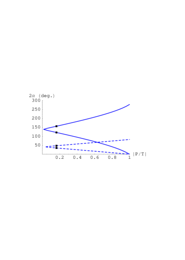
Figure 1: The angle $2\alpha$ as a function of the ratio $|P/T|$ for given values of the CP asymmetries (see text). The square dots correspond to the solutions with $|P/T|=0.16$.

is calculated from the theory. Similarly, Eq. (22) leads to two solutions for $2\alpha$ if $\delta$ is calculated from the theory. If both $|P/T|$ and $\delta$ can be estimated with sufficient precision, then in general only one value of $2\alpha$ will satisfy both Eqs. (21) and (22). Furthermore, the last discrete ambiguity $\alpha\to\pi+\alpha$ can be lifted by looking at the sign of $\sin\delta$, thanks to the equation

$$\mathrm{sign}(\sin\alpha)\times\mathrm{sign}(\sin\delta)=\mathrm{sign}(a_{\mathrm{dir}})$$ (23)

Recently, it has been argued that non-leptonic decays factorize in the heavy quark limit of QCD [4, 14], which should allow to compute the hadronic matrix elements in a model-independent way, up to $1/m_{b}$ corrections. Assuming for the moment that $|V_{td}/V_{ub}|$ is known, this formalism might give explicit predictions for the parameters $|P/T|$ and $\delta$. The procedure of how we get the angle $\alpha$ in practice is shown on Figs. (1)-(3).

As an example we assume $\alpha=1.36$. We take $|V_{td}/V_{ub}|=2.43$ and we obtain the observables $\sin 2\alpha_{\mathrm{eff}}$ and $a_{\mathrm{dir}}$ from the matrix elements calculated in Ref. [14]. We find $\sin 2\alpha_{\mathrm{eff}}=0.66$ and

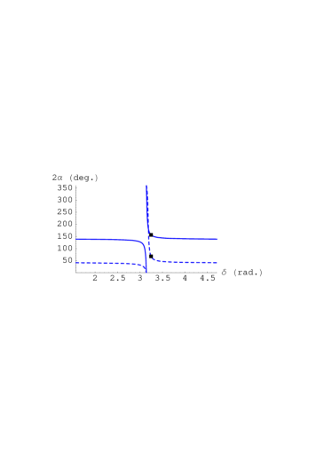
Figure 2: The angle $2\alpha$ as a function of the phase $\delta$ for given values of the CP asymmetries (see text). The square dots correspond to the solutions with $\delta=3.25$.

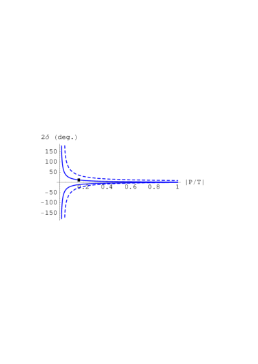
Figure 3: The phase $\delta$ as a function of the ratio $|P/T|$ for given values of the asymmetries (see text). The square dot corresponds to $(|P/T|=0.16,\delta=3.25)$ as given by factorization in the heavy quark limit.

$a_{\mathrm{dir}}=-0.03$. The latter numbers will of course be replaced by the actual ones once the CP measurements are available.

Let us now “forget” the value of the theoretical parameters ($\alpha$, $|V_{td}/V_{ub}|$ and the QCD matrix elements) that we have used, in such a way that we are only left with the knowledge of the two observables $\sin 2\alpha_{\mathrm{eff}}=0.66$ and $a_{\mathrm{dir}}=-0.03$: hopefully this will be the case in a near future. The question we would like to answer is how we could extract the value of $\alpha$ from the above observables. To this end, we plot the contours defined by Eqs. (21) and (22) in the $(|P/T|,2\alpha)$ and $(\delta,2\alpha)$ planes on Figs. (1) and (2) respectively. Note that these contours are completely model-independent.

From $|V_{td}/V_{ub}|=2.43$ and factorization in the heavy quark limit, we find $|P/T|=0.16$: this value is reported on the contours of Fig. (1), and four solutions for $2\alpha$ are determined in this way. Of course we have neglected both experimental and theoretical errors, and it remains to be investigated with which precision $2\alpha$ can be extracted from this approach. The uncertainty on the CKM angle depends on the experimental errors and the theoretical error on $|P/T|$.

Similarly, factorization predicts $\delta=3.25$, the value of which is reported on Fig. (2): this allows to select two possible values for $2\alpha$. One sees that only one value for the CKM angle is compatible with both the calculated $\delta$ and $|P/T|$ (the one corresponding tp the upper dot in both figures, with $2\alpha=156^{\circ}$). The remaining $\alpha\to\alpha+\pi$ ambiguity is lifted as indicated above by using Eq. (23) and $\sin\delta<0$ and $a_{\mathrm{dir}}<0$: we are left with a single value of the CP angle, $\alpha=1.36$, i.e. the value that we had as input for the calculation of the observables.

The fact that redundant information contained in $|P/T|$ and $\delta$ eliminates spurious solutions can be viewed in a different way: eliminating $\alpha$ between Eqs. (21) and (22), we obtain $2\delta$ as a function of $|P/T|$, the contour of which is drawn on Fig. (3). Any estimation of $(|P/T|,2\delta)$ should fall precisely on one of the branches: provided the various sources of error are controlled, this plot may constitute a good test of the theory. In case of a disagreement, this may be an indication of either the failure of the hadronic calculation, or New Physics.

Note that the knowledge of the ratio $|V_{td}/V_{ub}|$ is likely to be affected by still large uncertainties at the time where the CP experiments give first data. Actually, once the Standard Model is assumed, it is possible to express both $\alpha$ and $|V_{td}/V_{ub}|$ in terms of the Wolfenstein parameters $\rho$ and $\eta$, and solve directly the whole problem as contours in the $(\rho,\eta)$ plane [25].

This shows that with the help of the theory, the angle $\alpha$ can be determined without any discrete ambiguity in the general case. Of course, beside experimental uncertainties that will give some “width” to the contours of Figs. (1)-(3), we have to handle the theoretical errors associated with the calculation of $|P/T|$ and $\delta$, which both receive perturbative and non-perturbative $1/m_{b}$ corrections: the former are in principle calculable order by order in perturbation theory, while the latter may be much more difficult to control [14].

3.3 Conclusion

We have briefly reviewed part of the great theoretical progress concerning the determination of $\cos 2\beta$, and re-examined the extraction of the angle $\alpha$ in light of the recent QCD-based work on non-leptonic $B$-decays into two light mesons.

Acknowledgement

The authors acknowledge partial support from TMR-EC Contract No. ERBFMRX-CT980169.

References

- [1] Talks presented by G. Sciolla (BaBar Collaboration) and Y. Sakai (BELLE Collaboration), these proceedings.
- [2] T. Affolder et al. (CDF Collaboration), Phys. Rev. D61 (2000) 072005.
- [3] Talk presented by F. Parodi, these proceedings.
- [4] Talk presented by M. Neubert, these proceedings; M. Beneke, G. Buchalla, M. Neubert and C. T. Sachrajda, contribution to the conference ICHEP 2000, July 27-August 2, Osaka, Japan.
- [5] J. Charles, A. Le Yaouanc, L. Oliver, O. Pène and J.-C. Raynal, Phys. Rev. D58 (1998) 114021.
- [6] I. Dunietz, H. Quinn, A. Snyder and W. Toki, Phys. Rev. D43 (1991) 2193; A. S. Dighe, I. Dunietz, H. J. Lipkin and J. L. Rosner, Phys. Lett. B369 (1996) 144.
- [7] Cheng-Wei Chiang and Lincoln Wolfenstein, Phys. Rev. D61 (2000) 074031.
- [8] Y. Grossman, Y. Nir and M. P. Worah, Phys. Lett. B 07 (1997) 307.
- [9] G. C. Branco, L. Lavoura and J. P. Silva, CP Violation, Oxford University Press, Oxford, 1999.
- [10] Y. Grossman and H. R. Quinn, Phys. Rev. D56 (1997) 7259.
- [11] A. E. Snyder and H. R. Quinn, Phys. Rev. D48 (1993) 2139.
- [12] B. Kayser and D. London, Phys. Rev. D61 (2000) 116012.
- [13] The BaBar Physics Book, SLAC-R-504 (1998).
- [14] M. Beneke, G. Buchalla, M. Neubert and C. T. Sachrajda, Phys. Rev. Lett. 83 (1999) 1914; hep-ph/0006124.
- [15] J. Charles, A. Le Yaouanc, L. Oliver, O. Pène and J.-C. Raynal, Phys. Lett. B425 (1998) 375 and erratum-ibid B433 (1998) 441.
- [16] P. Colangelo, F. De Fazio, G. Nardulli, N. Paver and Riazuddin, Phys. Rev. D60 (1999) 033002.
- [17] A. S. Dighe, I. Dunietz and R. Fleischer, Eur. Phys. J. C6 (1999) 647.
- [18] Decays at the LHC, CERN-TH/2000-101, hep-ph/0003238.
- [19] B. Kayser, in Proceedings of the 32nd Rencontres de Moriond: Electroweak Interactions and Unified Theories, Les Arcs, France, edited by J. Trân Thanh Vân, Ed. Frontières (1997), p. 389; Ya. I. Azimov, JETP Lett. 50 (1989) 447, Phys. Rev. D42 (1990) 3705.
- [20] H. R. Quinn, T. Schietinger, J. P. Silva and A. E. Snyder, hep-ph/0008021 (2000).
- [21] Y. Grossman and D. Pirjol, J. High Energy Phys. 006 (2000) 029.
- [22] Results from the CLEO collaboration, presented at the conference ICHEP 2000, July 27-August 2, Osaka, Japan; from the BaBar collaboration, ibid.; from the BELLE collaboration, ibid.
- [23] M. Gronau, Phys. Rev. 63 (1989) 1451.
- [24] M. Gronau and D. London, Phys. Rev. Lett. 65 (1990) 3381.
- [25] J. Charles, Phys. Rev, D59 (1999) 054007.