Abstract

We analyze the electromagnetic form factors of the ground state baryon octet to fourth order in relativistic baryon chiral perturbation theory. Predictions for the $\Sigma^{-}$ charge radius and the $\Lambda$–$\Sigma^{0}$ transition moment are found to be in excellent agreement with the available experimental information. Furthermore, the convergence behavior of the hyperon charge radii is shown to be more than satisfactory.

Keywords: Baryon form factors, chiral perturbation theory

1 Introduction

Hadrons are composite objects, characterized by certain probe–dependent sizes. Their structure can be investigated by use of electron scattering (or the inverse process). The electromagnetic structure of the proton and the neutron has been investigated over decades, the present status of the data is e.g. discussed in [1]. In the non–perturbative low–energy region of QCD, baryon chiral perturbation theory can be used to calculate these form factors. In a recent paper [2] we have shown that relativistic baryon chiral perturbation theory (employing the so–called infrared regularization of [3]) supplemented by explicit vector meson contributions allows for a fairly precise description of these fundamental quantities for photon virtualities up to $Q^{2}\simeq 0.4$ GeV². The extension of these considerations to the three–flavor case is interesting for various reasons. First, the charge radius of the $\Sigma^{-}$ has recently been measured [4, 5] and thus gives a first glimpse of an electric hyperon form factor. Second, chiral SU(3) can be subject to large kaon/eta loop corrections, and the form factors offer another window to study the corresponding convergence properties. They might thus indicate whether or not the strange quark can be considered light and lead to a better understanding of SU(3) flavor breaking. Since the chiral expansion of the form factors is well under control in the two–flavor case, one can expect to encounter a reasonably well–behaved series also in the presence of the strange quark. This expectation is borne out by the results presented in this paper. Third, one can also address some questions concerning strangeness in the nucleon, more precisely, the role of kaon loops which in simple models let one expect sizeable contributions of strange operators. Fourth, a knowledge of certain hyperon form factors is mandatory to gain an understanding of kaon photo– and electroproduction off nucleons and light nuclei as measured at ELSA and TJNAF. We will come back to most of these topics in the present manuscript. In addition, these form factors have already been calculated in the so–called heavy–baryon approach [6, 7], which is a particular limit of the regularization procedure employed here. A direct comparison with the results of that approach can shed further light on the dynamics underlying the non–perturbative baryon structure, in particular the role of recoil corrections. As a final by–product, we can also readdress the issue of the convergence of the chiral expansion for the magnetic moments, which is much discussed in the recent literature [8, 9, 10, 11, 12].

The manuscript is organized as follows. In section 2 we briefly define the baryon form factors and the corresponding electromagnetic radii. The formalism to obtain the one–loop representation of the form factors is given in section 3. We heavily borrow from [2] and omit all lengthy formulae. The results are presented and discussed in section 4. Section 5 contains a short summary and outlook.

2 Baryon form factors

The structure of ground state octet baryons (denoted by ‘$B$’) as probed by virtual photons is parameterized in terms of two form factors each,

$$\langle B(p^{\prime})\,|\,{\cal J}_{\mu}\,|\,B(p)\rangle=e\,\bar{u}(p^{\prime})\,\biggl{\{}\gamma_{\mu}F_{1}^{B}(t)+\frac{i\sigma_{\mu\nu}q^{\nu}}{2m_{B}}F_{2}^{B}(t)\biggr{\}}\,u(p)\,,\quad B=p,n,\Lambda,\Sigma^{\pm},\Sigma^{0},\Xi^{-},\Xi^{0}\,,$$ (2.1)

with $t=q_{\mu}q^{\mu}=(p^{\prime}-p)^{2}$ the invariant momentum transfer squared, ${\cal J}_{\mu}$ the quark vector current, ${\cal J}_{\mu}=\bar{q}{\cal Q}\gamma_{\mu}q$ (${\cal Q}$ is the quark charge matrix and $q^{T}=(u,d,s)$), and $m_{B}$ the respective baryon mass. In electron scattering $t$ is negative and it is often convenient to define the positive quantity $Q^{2}=-t>0$. $F_{1}$ and $F_{2}$ are called the Dirac and the Pauli form factor, respectively, with the normalizations $F_{1}^{B}(0)=Q_{B}$, $F_{2}^{B}(0)=\kappa_{B}$. Here $\kappa_{B}$ denotes the anomalous magnetic moment. Eq. (2.1) has to be generalized for the $\Lambda$–$\Sigma^{0}$ transition form factors which are defined according to

$$\langle\Sigma^{0}(p^{\prime})\,|\,{\cal J}_{\mu}\,|\,\Lambda(p)\rangle=e\,\bar{u}(p^{\prime})\,\biggl{\{}\biggl{(}\gamma_{\mu}-\frac{m_{\Sigma^{0}}\!-\!m_{\Lambda}}{t}\,q_{\mu}\biggr{)}F_{1}^{\Lambda\Sigma^{0}}(t)+\frac{i\sigma_{\mu\nu}q^{\nu}}{m_{\Lambda}\!+\!m_{\Sigma^{0}}}F_{2}^{\Lambda\Sigma^{0}}(t)\biggr{\}}\,u(p)$$ (2.2)

(see also [13]). The form of the generalized Lorentz structure accompanying $F_{1}^{\Lambda\Sigma^{0}}(t)$ is required by current conservation (which becomes obvious by contracting eq. (2.2) with $q^{\mu}$ and applying the Dirac equation). Different definitions which all reduce to eq. (2.1) for $m_{\Sigma^{0}}\rightarrow m_{\Lambda}$ are possible, however, the one given here is preferable because it still requires the normalization $F_{1}^{\Lambda\Sigma^{0}}(0)=0$. One also uses the electric and magnetic Sachs form factors,

$$G_{E}(t)=F_{1}(t)+\displaystyle\frac{t}{4m_{B}^{2}}F_{2}(t)\,,\quad G_{M}(t)=F_{1}(t)+F_{2}(t)\,,$$ (2.3)

which are the quantities we will consider in the following. The slope of the form factors at $t=0$ is conventionally expressed in terms of a radius $\langle r^{2}\rangle^{1/2}$,

$$F(t)=F(0)\,\biggl{(}1+\displaystyle\frac{1}{6}\langle r^{2}\rangle\,t+\ldots\biggr{)}$$ (2.4)

($F$ being a genuine symbol for any of the four electromagnetic baryon form factors), and the mean square radius of this charge distribution is given by

$$\langle r^{2}\rangle=4\pi\,\int_{0}^{\infty}dr\,r^{2}\rho(r)=\displaystyle\frac{6}{F(0)}\displaystyle\frac{dF(t)}{dt}\biggr{|}_{t=0}~{}.$$ (2.5)

Eq. (2.5) can be used for all form factors except for the electric ones of the neutral baryons which vanish at $t=0$. In these cases, one simply drops the normalization factor $1/F(0)$ and defines e.g. the neutron charge radius via

$$\langle(r_{E}^{n})^{2}\rangle\,=6\,\displaystyle\frac{dG_{E}^{n}(t)}{dt}\biggr{|}_{t=0}~{}.$$ (2.6)

3 Formalism

In this section, we spell out the details necessary to extend the SU(2) calculation of [2] to the three–flavor case. We work in relativistic baryon chiral perturbation theory, employing infrared regularization (IR). For details on this procedure, we refer to [3, 2]. Although the presence of different pseudo–Goldstone bosons with unequal masses entails more general loop functions than those encountered in [2], we refrain from tabulating these here. They will become available in [14]. We only spell out the various terms of the effective chiral Lagrangian underlying the calculation. Again we do not give the final formulae for the form factors since these are rather lengthy, but instead refer to [14].

3.1 Effective Lagrangian

The chiral effective Goldstone boson Lagrangian is given by

$${\cal L}_{\phi\phi}^{(2)}=\frac{F^{2}}{4}\langle u_{\mu}u^{\mu}+\chi_{+}\rangle~{},$$ (3.1)

where the octet of Goldstone boson fields is collected in the SU(3) valued matrix $U(x)=u^{2}(x)$, and the chiral vielbein is related to $u$ via $u_{\mu}=i\{u^{\dagger},\nabla_{\mu}u\}$. $\nabla_{\mu}$ is the covariant derivative acting on the pion fields including external vector ($v_{\mu}$) and axial ($a_{\mu}$) sources, $\nabla_{\mu}U=\partial_{\mu}U-i\bigl{(}v_{\mu}+a_{\mu}\bigr{)}U+iU\bigl{(}v_{\mu}-a_{\mu}\bigr{)}$. The mass term is included in the field $\chi_{+}$ via the definitions $\chi=2B(s+i\,p)$ and $\chi_{+}=u^{\dagger}\chi u^{\dagger}+u\chi^{\dagger}u$, with $s$ and $p$ being scalar and pseudoscalar sources, respectively. $s$ includes the quark mass matrix, $s={\rm diag}(m_{u},m_{d},m_{s})+\ldots$ . We will work in the isospin limit, $m_{u}=m_{d}=\hat{m}$. $B=|\langle 0|\bar{q}q|0\rangle|/F^{2}$ measures the strength of the symmetry violation, and we assume the standard scenario, $B\gg F$. Furthermore, $\langle\ldots\rangle$ denotes the trace in flavor space. The mass term leads to the well–known lowest–order (isospin symmetric) mass formulae for pions, kaons, and the eta, which enter the description of the baryon form factors via loop contributions. We would like to point out that the mass differences between the Goldstone bosons yield the leading–order SU(3) breaking effect for these form factors. For numerical evaluation, we will use $M_{\pi}=139.57$ MeV, $M_{K}=493.68$ MeV (the charged pion and kaon masses), and $M_{\eta}=547.45$ MeV. Furthermore, it is legitimate to differentiate between different decay constants $F_{\pi}$, $F_{K}$, $F_{\eta}$ in the treatment of the chiral loops as these differences are of higher order. We will use $F_{\pi}=92.4$ MeV, $F_{K}/F_{\pi}=1.22$, $F_{\eta}/F_{\pi}=1.3$ (see [15] and, for a more recent determination of $F_{K}/F_{\pi}$, [16]). The main motivation for not using a common decay constant is the comparison to the SU(2) results for the proton and neutron form factors, where we do not want to suggest an SU(3) effect which is only due to a numerically different treatment of the pion loops.

The meson–baryon Lagrangian at leading order reads

$${\cal L}_{\phi B}^{(1)}=\langle\bar{B}\left(iD\!\!\!\!/-m\right)B\rangle+\frac{D/F}{2}\,\langle\bar{B}\gamma^{\mu}\gamma_{5}\left(u_{\mu},B\right)_{\pm}\rangle~{},$$ (3.2)

where the matrix–valued field $B$ collects the ground state octet baryons and $D$ and $F$ are the axial vector coupling constants. For these, we will use the values $D=0.80$, $F=0.46$ extracted from hyperon decays [17], which obey the SU(2) constraint $D+F=g_{A}=1.26$. Here, $m$ denotes the average baryon mass in the chiral limit. To this order, the photon field only couples to the charge of the baryon. It resides in the chiral covariant derivative, $D_{\mu}B=\partial_{\mu}B+[\Gamma_{\mu},B]$, with the chiral connection given by $\Gamma_{\mu}=\frac{1}{2}\bigl{[}u^{\dagger},\partial_{\mu}u\bigr{]}-\frac{i}{2}u^{\dagger}(v_{\mu}+a_{\mu})u-\frac{i}{2}u(v_{\mu}-a_{\mu})u^{\dagger}$.

Coupling constants from the second–order meson–baryon Lagrangian are needed both at tree level and in one–loop graphs. The following terms are required in our calculation:

$${\cal L}_{\phi B}^{(2)} = b_{D/F}\langle\bar{B}(\chi_{+},B)_{\pm}\rangle+\frac{b_{6}^{D/F}}{8m}\langle\bar{B}\sigma^{\mu\nu}(F_{\mu\nu}^{+},B)_{\pm}\rangle$$ (3.3)

$$+\frac{i}{2}\sigma^{\mu\nu}\biggl{\{}b_{9}\langle\bar{B}u_{\mu}\rangle\langle u_{\nu}B\rangle+b_{10/11}\langle\bar{B}([u_{\mu},u_{\nu}],B)_{\pm}\rangle\biggr{\}}~{}.$$

Here, $F^{+}_{\mu\nu}=u^{\dagger}F_{\mu\nu}u+uF_{\mu\nu}u^{\dagger}$, and $F_{\mu\nu}=\partial_{\mu}A_{\nu}-\partial_{\nu}A_{\mu}$ is the conventional photon field strength tensor. The $b_{i}$ are the so–called low–energy constants (LECs) which encode information about the more massive states not contained in the effective field theory or other short–distance effects. These parameters have to be pinned down by using some data. In principle there is also a term $\sim b_{0}\,\langle\bar{B}B\rangle\langle\chi_{+}\rangle$ which amounts to a quark mass renormalization of the common octet mass $m$. This, however, cannot be disentangled from $m$ without further information (like the pion–nucleon $\sigma$ term), and it is sufficient for our purpose to absorb this term in $m$. The couplings $b_{D/F}$ yield the leading SU(3) breaking effects in the baryon masses. Again, these affect the form factors via various loop contributions. A best fit to the octet masses results in $m_{N}=0.942$ GeV, $m_{\Lambda}=1.111$ GeV, $m_{\Sigma}=1.192$ GeV, $m_{\Xi}=1.321$ GeV (for $m=1.192$ GeV, $b_{D}=0.060$ GeV^-1, $b_{F}=-0.190$ GeV^-1), compared to the experimental values $m_{N}=0.939$ GeV, $m_{\Lambda}=1.116$ GeV, $m_{\Sigma}=1.193$ GeV, $m_{\Xi}=1.318$ GeV (where the average masses within the respective isospin multiplets have been taken). We consider this accurate enough to put all baryon masses to their experimental values in the numerical evaluation. In any third–order calculation, however, no mass splitting is present, hence the baryon mass parameter will always be put to the average baryon mass $\bar{m}=1.151$ GeV in this case. It has been discussed in detail in [3, 2] how to fix the omnipresent mass scale $\lambda$ which has to be introduced in loop diagrams treated in dimensional regularization. It was argued that in an SU(2) calculation, the nucleon mass serves as a natural mass scale. Here we consider it natural to set $\lambda=\bar{m}$. The LECs $b_{6}^{D/F}$ parameterize the leading magnetic photon couplings to the baryons and will be fitted to the magnetic moments. Finally, the LECs $b_{9/10/11}$ accompany second–order couplings of the various pseudo–Goldstone bosons to baryons and enter the form factors via (tadpole) loop contributions. Their values have been estimated based on the resonance saturation hypothesis in [9], however, the results used there do not satisfy the SU(2) constraint $2(b_{10}+b_{11})=c_{4}\approx 3.4$ GeV^-1. The latter value is well–established, consistently determined from resonance saturation [18] and fits to pion–nucleon scattering [19, 20]. The discrepancy between both determinations can be traced back to different treatments of the $\Delta$ contribution in [9] and [18]. Adjusting this, we will use the values $b_{9}=1.36$ GeV^-1, $b_{10}=1.24$ GeV^-1, $b_{11}=0.46$ GeV^-1. As we would like to specify the uncertainty of our predictions based on these estimates later on, we attribute some errors to these LECs. As an indication we regard the change of a LEC when fitting it within chiral amplitudes of different orders. This change is about 1.0 GeV^-1 for $c_{4}$ when going from second to third order in $\pi N$ scattering (see [21] for a second order fit). We assume that this change should be a factor of 2 smaller when proceeding from third to fourth order such that, due to the different normalization of the SU(3) couplings, we set $\Delta b_{9/10/11}=0.25$ GeV^-1.

The only terms needed from the third order Lagrangian are those entering the electric (charge) radii of the baryons,

$${\cal L}_{\phi B}^{(3)} = \frac{id_{101/102}}{2m}\biggl{\{}\langle\bar{B}\Bigl{(}[D^{\mu},F_{\mu\nu}^{+}],[D^{\nu},B]\Bigr{)}_{\mp}\rangle+{\rm h.c.}\biggr{\}}~{}.$$ (3.4)

$d_{101},\,d_{102}$ have to be fitted to the charge radii of proton and neutron.

At fourth order, two types of coupling constants appear which are of relevance for our calculation: two couplings entering the magnetic radii, and seven couplings proportional to a quark mass insertion contributing to the magnetic moments,

$${\cal L}_{\phi B}^{(4)} = \frac{\alpha_{1/2}}{8}\langle\bar{B}\sigma^{\mu\nu}\Bigl{(}[F_{\mu\nu}^{+},B],\chi_{+}\Bigr{)}_{\mp}\rangle+\frac{\alpha_{3/4}}{8}\langle\bar{B}\sigma^{\mu\nu}\Bigl{(}\{F_{\mu\nu}^{+},B\},\chi_{+}\Bigr{)}_{\mp}\rangle$$ (3.5)

$$+\frac{\beta_{1}}{8}\langle\bar{B}\sigma^{\mu\nu}B\rangle\langle\chi_{+}F_{\mu\nu}^{+}\rangle+\frac{\tilde{b}_{6}^{D/F}}{8}\langle\chi_{+}\rangle\langle\bar{B}\sigma^{\mu\nu}(F_{\mu\nu}^{+},B)_{\pm}\rangle$$

$$-\frac{\eta_{1/2}}{2}\langle\bar{B}\sigma^{\mu\nu}\Bigl{(}[D_{\lambda},[D^{\lambda},F_{\mu\nu}^{+}]],B\Bigr{)}_{\mp}\rangle~{}.$$

As indicated by the notation, the terms $\sim\tilde{b}_{6}^{D/F}$ only amount to a quark mass renormalization of the leading magnetic couplings and will therefore be absorbed into $b_{6}^{D/F}$. The LECs $\alpha_{1-4}$, $\beta_{1}$, however, incorporate explicit breaking of SU(3) symmetry in the magnetic moments and will be fitted to the octet moments. $\eta_{1/2}$ will be adjusted to the magnetic radii of proton and neutron.

While there are, all in all, quite some LECs to be fitted in order to describe all electromagnetic form factors, it is important to point out that all these LECs are, on general grounds, expected to be of order 1 (with the appropriate mass dimensions in powers of GeV: as the baryonic scale is of the order of 1 GeV, it is not necessary to normalize the LECs appropriately).

3.2 Chiral expansion of the baryon form factors

The chiral expansion of a form factor $F$ consists of two contributions, tree and loop graphs. The tree graphs comprise the lowest–order diagram with fixed coupling (the baryon charge) as well as counterterms from the second–, third–, and fourth–order Lagrangians. As one–loop graphs we have both those with just lowest–order couplings and those with exactly one insertion from ${\cal L}_{\phi B}^{(2)}$. The pertinent tree and loop graphs are depicted in fig. 1 (we have not shown the diagrams leading to wave function renormalization). We refrain from giving the explicit expressions here but we mention that in the limit of a heavy strange quark, we recover the SU(2) results of [2]. Also, the heavy–baryon (HB) results of [6] can be obtained straightforwardly as detailed in [2].

4 Results and discussion

We first discuss the issues concerning the magnetic moments and the electromagnetic radii in some detail. This can be done within the ‘pure’ chiral expansion. Then we turn to the full momentum dependence of the various form factors for photon virtualities up to $Q^{2}=0.3$ GeV². To this end we have to include vector mesons as active degrees of freedom in a chirally symmetric manner.

4.1 Magnetic moments

The issue of convergence of the magnetic moments in chiral perturbation theory (ChPT) has been discussed amply in the literature, with or without inclusion of the decuplet [8, 9, 10, 11, 12]. We wish to compare the convergence behavior in the heavy–baryon and the infrared regularization scheme. Table 1 shows the best fits to the various orders. The strategy is always to fit the seven experimentally measured static moments ($\mu_{\Sigma^{0}}$ has not been measured so far, in the theoretical predictions it is always given by $\mu_{\Sigma^{0}}=(\mu_{\Sigma^{+}}+\mu_{\Sigma^{-}})/2$ according to isospin symmetry) and to predict the transition moment $\mu_{\Lambda\Sigma^{0}}$. At second and third order, only the two leading–order couplings $b_{6}^{D/F}$ are free parameters, which results in best fits of varying quality, whereas at fourth order the additional five couplings allow for an exact fit of all seven static moments. At second/third order, we have performed an unweighted fit, hence simply minimizing $\chi^{2}=\sum(\mu_{\rm th}-\mu_{\rm exp})^{2}$. The $\chi^{2}$ values given in table 1 thus only serve to indicate the relative quality of the fits.

		HB		IR
	${\cal O}(q^{2})$	${\cal O}(q^{3})$	${\cal O}(q^{4})$	${\cal O}(q^{3})$	${\cal O}(q^{3})^{*}$	${\cal O}(q^{4})$	exp.
$p$	2.56	2.97	2.793	2.61	2.20	2.793	$2.793\pm 0.000$
$n$	$-$1.60	$-$2.53	$-$1.913	$-$1.69	$-$2.59	$-$1.913	$-1.913\pm 0.000$
$\Lambda$	$-$0.80	$-$0.45	$-$0.613	$-$0.76	$-$0.65	$-$0.613	$-0.613\pm 0.004$
$\Sigma^{+}$	2.56	2.21	2.458	2.53	2.41	2.458	$2.458\pm 0.010$
$\Sigma^{0}$	0.80	0.45	0.649	0.76	0.65	0.649	—
$\Sigma^{-}$	$-$0.97	$-$1.32	$-$1.160	$-$1.00	$-$1.12	$-$1.160	$-1.160\pm 0.025$
$\Xi^{0}$	$-$1.60	$-$0.78	$-$1.250	$-$1.51	$-$1.20	$-$1.250	$-1.250\pm 0.014$
$\Xi^{-}$	$-$0.97	$-$0.56	$-$0.651	$-$0.93	$-$1.33	$-$0.651	$-0.651\pm 0.003$
$\Lambda\Sigma^{0}$	1.38	1.65	$1.46\pm 0.01$	1.41	1.81	$1.61\pm 0.01$	$\pm 1.61\pm 0.08$
$b^{D}_{6}$	2.40	5.27	$4.56\pm 0.24$	3.65	5.18	$4.21\pm 0.20$
$b^{F}_{6}$	0.77	2.92	$1.65\pm 0.19$	1.73	0.56	$1.64\pm 0.18$
$\alpha_{1}$	—	—	$-1.00\pm 0.26$	—	—	$0.32\pm 0.28$
$\alpha_{2}$	—	—	$1.35\pm 0.29$	—	—	$-0.08\pm 0.18$
$\alpha_{3}$	—	—	$-0.85\pm 0.30$	—	—	$2.14\pm 0.28$
$\alpha_{4}$	—	—	$0.95\pm 0.22$	—	—	$0.05\pm 0.19$
$\beta_{1}$	—	—	$-2.46\pm 0.33$	—	—	$-3.39\pm 0.34$
$\chi^{2}$	0.46	0.76	0.00	0.28	1.28	0.00

Table 1: Analysis of the magnetic moments (in units of nuclear magnetons (n.m.)) to different chiral orders. The various best–fit values for the leading order magnetic couplings $b^{D/F}_{6}$ and the SU(3) breaking couplings $\alpha_{1-4}$, $\beta_{1}$ are given as well. $b^{D/F}_{6}$ are dimensionless, $\alpha_{1-4}$, $\beta_{1}$ are given in units of GeV^-3. Errors for fourth–order results display the uncertainty due to $\Delta b_{9/10/11}$. For the definition of $\chi^{2}$, see text.

It has frequently been noted before that the inclusion of leading loop corrections in the magnetic moments tends to worsen the leading–order results. This is seen here in the third–order heavy–baryon results. Within the infrared regularization scheme, however, it is even disputable which contributions to count as third order: the leading contributions stem from diagram (6) in fig. 1; summing up only the $1/m$–corrections to this graph yields the fit in the column denoted by ‘${\cal O}(q^{3})$’ and shows an improvement not only over the heavy–baryon result, but also over the leading order fit. However, defining any one–loop diagram with no higher–order insertions to be of third order, one also has to include diagram (5) in fig. 1 (which only contributes at fourth order in strict chiral power counting). These contributions are large and worsen the fit even over the third–order heavy–baryon one, see the column denoted by ‘${\cal O}(q^{3})^{*}$’. Especially the magnetic moments of proton, neutron, and $\Xi^{-}$ are not described to any acceptable accuracy in this case. We note furthermore that the fitted values for the leading–order couplings vary considerably among the different fits. Regarding these as indicators for convergence, we again find that the ‘${\cal O}(q^{3})$’ result is much closer to the fourth–order fit than the ‘${\cal O}(q^{3})^{*}$’ one.

At fourth order, we can compare the two predictions for the transition moment $\mu_{\Lambda\Sigma^{0}}$. In both cases, we have indicated the uncertainty of these predictions due to the estimated uncertainties of the couplings $b_{9/10/11}$, which turns out to be much smaller than the experimental error of $\Delta\mu_{\Lambda\Sigma^{0}}^{\rm exp}=0.08$. It is remarkable that the prediction for this physical quantity is so stable under variation of $b_{9/10/11}$, although the fit values for the individual couplings given in table 1 vary considerably. While the heavy–baryon result is about two standard deviations off, the relativistic one ($\mu_{\Lambda\Sigma^{0}}=1.606\pm 0.008$ n.m.) yields exactly the experimental result (to be precise, experimentally only $|\mu_{\Lambda\Sigma^{0}}|$ is known). We note furthermore that, while the values for the leading–order magnetic couplings $b_{6}^{D/F}$ are fairly close in the two different schemes, those for the SU(3) breaking couplings show no similarity at all. This clearly displays the fact that $1/m$ corrections to the various loop diagrams are sizeable even beyond fourth order.

4.2 Electric radii

The electric (or charge) radius of any baryon is, according to eq. (2.3), given by the sum of the Dirac radius and the so–called Foldy term,

$$\langle r_{E}^{2}\rangle=\langle r_{1}^{2}\rangle+\frac{3\,\kappa_{B}}{2\,m_{B}^{2}}~{}.$$ (4.1)

Phenomenologically the Foldy term is hence well–known for all ground state octet baryons from the experimental information on the magnetic moments. What remains to be predicted from any kind of theory or model, as independent quantities, are the Dirac radii. We have therefore always replaced the chiral representation of the Foldy term by the exact value given by experiment. This is legitimate at any chiral order, as the difference is always subleading. Doing otherwise would partly import the well–known problematic convergence properties of the magnetic moments to the description of the electric radii.

	HB		IR
	${\cal O}(q^{3})$	${\cal O}(q^{4})$	${\cal O}(q^{3})$	${\cal O}(q^{4})$	exp.
$p$	0.717	0.717	0.717	0.717	0.717
$n$	$-$0.113	$-$0.113	$-$0.113	$-$0.113	$-$0.113
$\Lambda$	0.14	0.00	0.05	0.11$\pm$0.02	—
$\Sigma^{+}$	0.59	0.72	0.63	0.60$\pm$0.02	—
$\Sigma^{0}$	$-$0.14	$-$0.08	$-$0.05	$-$0.03$\pm$0.01	—
$\Sigma^{-}$	0.87	0.88	0.72	0.67$\pm$0.03	0.60$\pm$0.08$\pm$0.08 [5]
					0.91$\pm$0.32$\pm$0.40 [4]
$\Xi^{0}$	0.36	0.08	0.15	0.13$\pm$0.03	—
$\Xi^{-}$	0.67	0.75	0.56	0.49$\pm$0.05	—
$\Lambda\Sigma^{0}$	$-$0.10	$-$0.09	0.00	0.03$\pm$0.01	—
$d_{101}$	$-$0.84	$-$0.34	$-$0.44	$-$0.15
$d_{102}$	1.20	1.64	1.57	1.64

Table 2: Predictions for the electric radii $\langle r_{E}^{2}\rangle$ [fm²]. The various best–fit values for the pertinent counterterms $d_{101}$, $d_{102}$ are given as well (in units of GeV^-2). The experimental values for the proton and neutron are taken from the dispersion theoretical studies [23, 24]. The errors for the relativistic fourth order predictions display the uncertainty due to $\Delta b_{6}^{D/F}$. The errors for the experimental $\Sigma^{-}$ radius values refer to statistical (first) and systematic (second) errors.

The chiral representations of the electric radii of the baryon octet, both at third and fourth order, involve exactly two low–energy constants, $d_{101}$ and $d_{102}$. These can readily be fitted to the charge radii of proton and neutron, such that all others can be predicted. Table 2 shows these predictions for third– and fourth–order calculations, both in the heavy–baryon and the infrared regularization formalism. The fourth column shows the predictions according to the fourth order relativistic calculation together with errors which reflect some theoretical uncertainty: even with the Foldy term fixed, some uncertainty inherited from the description of the magnetic moments remains. Indeed, though kinematically suppressed (i.e. of higher than fourth order in strict chiral power counting), the loop corrections to the anomalous magnetic couplings, see diagram (10) in fig. 1, contribute to the Dirac radius. We employ the values for $b_{6}^{D/F}$ obtained from the best fit to the magnetic moments at fourth order, $b_{6}^{D}=4.21$ and $b_{6}^{F}=1.64$, see table 1. In order to get an estimate of the uncertainty due to these LECs, we again assume an error of about half of the change when fitting them at third and fourth order, thus assigning $\Delta b_{6}^{D/F}=0.5$. Table 2 shows that this uncertainty is (relatively) small, as would be expected. We would like to stress however that this error only indicates one particular effect. An estimate of the complete uncertainty due to higher–order contributions is hardly feasible (or, due to the appearance of new unknown couplings, indeed impossible). Finally, the uncertainties due to the experimental errors on the magnetic moments entering the Foldy term are yet one order of magnitude smaller.

With regard to convergence only, i.e. exclusively to the numerical changes when going from third to fourth order, the infrared regularization scheme yields overall considerable improvement over the heavy–baryon results, especially for $\Lambda$, $\Sigma^{+}$, and $\Xi^{0}$. This improvement can also be seen in the behavior of the fitted values of $d_{101}$ and $d_{102}$, also given in table 2, which are more stable in the relativistic scheme. What is more important though is that both the absolute values and the trends within the two schemes are entirely different for some hyperons. E.g. for the $\Sigma^{-}$ radius, the only hyperon radius on which experimental information exists, the heavy–baryon values are very stable at 0.87–0.88 fm², but deviate sizeably from the radius given by the SELEX collaboration [5], $\langle(r_{E}^{\Sigma^{-}})^{2}\rangle=0.60\pm 0.08({\rm stat.})\pm 0.08({\rm syst.})$ fm² (the pioneering WA89 measurement [4] is not precise enough to favor any of the theoretical predictions). In the relativistic scheme however, the third–order value is already within this error range, with the fourth–order one even closer to the central value. Similarly for the other charged hyperons $\Sigma^{+}$ and $\Xi^{-}$, the fourth–order corrections increase the third–order predictions in the heavy–baryon case, but reduce them in the relativistic scheme. We also note that only the relativistic predictions show the hierarchy in the size of the electric radii expected from naive quark model considerations, $\langle(r_{E}^{p})^{2}\rangle>\langle(r_{E}^{\Sigma^{\pm}})^{2}\rangle>\langle(r_{E}^{\Xi^{-}})^{2}\rangle$. The sizeable difference between the $\Sigma^{+}$ and $\Sigma^{-}$ radii at third order in the heavy–baryon scheme is largely reduced in the relativistic results, leaving only a 10% effect at fourth order. For the neutral hyperons, all predictions are consistent as far as the signs of the radii are concerned (with the exception of the radius of the $\Lambda$–$\Sigma^{0}$ transition form factor), yielding positive radii for the $\Lambda$ and $\Xi^{0}$ hyperons, and a negative radius for the $\Sigma^{0}$. Quantitatively, the relativistic fourth–order calculation predicts radii of a size very similar to that of the neutron for $\Lambda$ and $\Xi^{0}$, and a $\Sigma^{0}$ radius of about another factor of 3 smaller.

To conclude this section, we would like to comment on the issue of SU(3) breaking in the electric radii. In contrast to the calculation of the magnetic moments to fourth order, the electric radii to this order do not contain any operators which break SU(3) at tree level (compare the LECs $\alpha_{1-4},\,\beta_{1}$ in eq. (3.5) in the magnetic sector), therefore all SU(3) breaking effects are created ‘dynamically’ via mass splittings in the loop diagrams. The leading (and dominating) effect is the pion–kaon mass difference. We remind the reader that SU(3) symmetry would give the hyperon radii in terms of the proton/neutron radii according to

$$\langle(r_{E}^{\Sigma^{+}})^{2}\rangle\!\! = \!\!\langle(r_{E}^{p})^{2}\rangle~{},\qquad\langle(r_{E}^{\Sigma^{-}})^{2}\rangle\,=\,\langle(r_{E}^{\Xi^{-}})^{2}\rangle\,=\,\langle(r_{E}^{p})^{2}\rangle+\langle(r_{E}^{n})^{2}\rangle~{},$$

$$2\,\langle(r_{E}^{\Lambda})^{2}\rangle\!\! = \!\!-2\,\langle(r_{E}^{\Sigma^{0}})^{2}\rangle\,=\,\langle(r_{E}^{\Xi^{0}})^{2}\rangle\,=\,-\frac{2}{\sqrt{3}}\,\langle(r_{E}^{\Lambda\Sigma^{0}})^{2}\rangle\,=\,\langle(r_{E}^{n})^{2}\rangle~{}.$$ (4.2)

It is obvious that SU(3) breaking due to the large kaon mass changes this pattern considerably: exact SU(3) predicts $\langle(r_{E}^{\Sigma^{+}})^{2}\rangle>\langle(r_{E}^{\Sigma^{-}})^{2}\rangle$ which is reversed in all four ChPT results presented above. In addition, it changes the sign of all charge radii for neutral hyperons. The size of the additional SU(3) breaking due to the mass splitting in the baryon octet, see diagrams (5^∗)–(7^∗) in fig. 1, can be seen by comparing the predictions at third and fourth order in the relativistic framework, the change being mainly due to these mass differences (in fact, in terms of strict chiral power counting, this is the only new effect at fourth order apart from $1/m$ corrections to third order loops). The net effect is a further moderate reduction of the charged hyperon radii. Among the neutral particles, only the $\Lambda$ radius shows a sizeable correction. Going to fifth order, one would obtain a large amount of additional SU(3) breaking effects (e.g. in the meson–baryon coupling constants or ‘explicit’ breaking in the charge radii via contact terms) none of which is quantifiable to sufficient accuracy. We thus regard our (fourth–order relativistic) predictions as the best one is ever likely to achieve in any ChPT approach.

4.3 Magnetic radii

As the electric radii, the magnetic radii at fourth order include two parameters (labeled $\eta_{1/2}$ in eq. (3.5)) which can be fitted to the respective proton and neutron data (taken here from the dispersive analysis [23, 24]) in order to yield predictions for the hyperons. However, in contrast to the electric case, here loops proportional to other rather poorly known LECs ($b_{9/10/11}$) contribute significantly. As there are no further measurements of magnetic radii which would allow to fit these, the most transparent thing to do is to indicate the uncertainty following from this poor knowledge. Table 3 shows these uncertainties, based on $\Delta b_{9/10/11}=0.25$ GeV^-1 (which are assumed to be uncorrelated errors). Again, this is only one particular effect and does not reflect all possible uncertainties due to higher–order contributions. In addition, errors on these couplings were also only roughly estimated, such that they could even be larger.

	${\cal O}(q^{4})$ ${\rm HB}$	${\cal O}(q^{4})$ ${\rm IR}$	exp.
$p$	0.699	0.699	0.699
$n$	0.790	0.790	0.790
$\Lambda$	0.30$\pm$0.11	0.48$\pm$0.09	—
$\Sigma^{+}$	0.74$\pm$0.06	0.80$\pm$0.05	—
$\Sigma^{0}$	0.20$\pm$0.10	0.45$\pm$0.08	—
$\Sigma^{-}$	1.33$\pm$0.16	1.20$\pm$0.13	—
$\Xi^{0}$	0.44$\pm$0.15	0.61$\pm$0.12	—
$\Xi^{-}$	0.44$\pm$0.20	0.50$\pm$0.16	—
$\Lambda\Sigma^{0}$	0.60$\pm$0.10	0.72$\pm$0.10	—
$\eta_{1}$	0.26$\pm$0.10	0.69$\pm$0.10
$\eta_{2}$	$-$0.02$\pm$0.21	0.72$\pm$0.21

Table 3: Predictions for the magnetic radii $\langle r_{M}^{2}\rangle$ [fm²]. The various best–fit values for the pertinent counterterms $\eta_{1}$, $\eta_{2}$ are given as well (in units of GeV^-3). The errors display the uncertainty due to $\Delta b_{9/10/11}$.

Nevertheless, we consider the errors in table 3 indicative enough to state that the magnetic radii can be predicted only to much lower accuracy than the electric ones. Given the sizeable uncertainties, there is no significant discrepancy between the heavy–baryon and the relativistic predictions (with the exception of the $\Sigma^{0}$). The general trend is an increase of most magnetic radii in the relativistic scheme compared to the heavy–baryon results, where the central values are surprisingly small for some hyperons ($\Lambda$, $\Sigma^{0}$). The values for the LECs $\eta_{1/2}$, however, are completely different. This indicates large SU(3) symmetric loop contributions that have to be canceled by these counterterms. This does not come as a surprise if one remembers what is known about loop contributions to the magnetic moments. Note that with regard to the values for the SU(3) breaking terms in the magnetic moments given in section 4.1, none of the fourth–order couplings can be fixed in agreement with both schemes. SU(3) breaking is large, as a completely SU(3) symmetric treatment of the magnetic form factors (moments and radii) would imply

$$\langle(r_{M}^{\Sigma^{+}})^{2}\rangle\!\! = \!\!\langle(r_{M}^{p})^{2}\rangle~{},$$

$$\langle(r_{M}^{\Sigma^{-}})^{2}\rangle\!\! = \!\!\langle(r_{M}^{\Xi^{-}})^{2}\rangle\,=\,\frac{\mu_{p}\langle(r_{M}^{p})^{2}\rangle+\mu_{n}\langle(r_{M}^{n})^{2}\rangle}{\mu_{p}+\mu_{n}}~{},$$

$$\langle(r_{M}^{\Lambda})^{2}\rangle\!\! = \!\!\langle(r_{M}^{\Sigma^{0}})^{2}\rangle\,=\,\langle(r_{M}^{\Lambda\Sigma^{0}})^{2}\rangle\,=\,\langle(r_{M}^{n})^{2}\rangle~{}.$$ (4.3)

In contrast to these, the values in table 3 show no clear pattern. The magnetic radius of the $\Sigma^{-}$ is remarkable in being much larger than all other radii, electric or magnetic. Such an effect, albeit less dramatic, is also found in some lattice studies, see e.g. [13]. (This study also predicts relatively small magnetic radii for $\Lambda$ and $\Xi^{-}$ as we do, though not for the $\Sigma^{0}$.) As in the case of the electric radii, improvement of these predictions in the framework of ChPT is hardly feasible as higher order corrections would include numerous unknown SU(3) breaking effects.

4.4 $Q^{2}$–dependence of the form factors

In [2] it was shown that the complete relativistic chiral one–loop representation fails to describe the $Q^{2}$–dependence of the ‘large’ form factors (i.e. those not vanishing at $Q^{2}=0$) already at rather low $Q^{2}$. As a remedy, it was demonstrated that the inclusion of dynamical vector mesons, used in an antisymmetric tensor representation and coupled to nucleons/pions/photons in a chirally invariant fashion, yields a very good description of all electromagnetic nucleon form factors up to about 0.4 GeV². Certainly, in order to obtain reasonable predictions for the $Q^{2}$–dependence of the hyperon form factors, one has to proceed likewise here. The necessary formalism and the definitions of all pertinent couplings are presented in great detail in [2]. Of course one has to assume SU(3) symmetric vector meson couplings to the baryons, which are then fully determined by the values for the vector meson nucleon couplings as given in [23]. As these transform in the same way as the contact terms, replacing part of the latter by explicit vector meson contributions on tree level affects in no way the predictions for the hyperon radii.

The fourth order results for the electric form factors of proton and neutron, including vector meson effects, are shown in figs. 2 and 3, respectively, the former divided by the dipole form factor. For comparison we show the equivalent SU(2) results given in [2] and the dispersion theoretical fits from [23, 24]. In both cases the difference between the SU(2) and SU(3) descriptions is very small, though the SU(3) one is slightly worse. From such small differences one concludes that not much room is left for a strangeness contribution via kaon loops, as simple meson cloud models seem to indicate. Strangeness as hidden in the $\phi$–meson component or from higher mass states encoded in the value of the LECs $d_{101/102}$ cannot be separated from the analysis presented here. To completely disentangle the strangeness contribution to a given form factor, a full flavor decomposition is necessary. For that, one also has to calculate the singlet form factors since the electromagnetic current is only sensitive to the triplet and octet current components.

Fig. 4 shows the electric form factors of all charged hyperons (those of the negative ones with sign reversed). They all show a $Q^{2}$–dependence qualitatively similar to that of the proton charge form factor, the quantitative difference being due to their different sizes as determined by the radii. In all cases, the vector meson effects contribute a large part of the curvature which is far too small for the proton in a purely chiral representation. The neutral hyperon form factors are shown in fig. 5 in comparison to the neutron electric form factor. Similar to what was found for the latter in [2], the vector meson effects largely cancel for all charge form factors of neutral hyperons. Apart from the neutron, only the $\Lambda$–$\Sigma^{0}$ transition form factor shows significant curvature, the ones for $\Lambda$, $\Sigma^{0}$, and $\Xi^{0}$ are dominated by the radius term and display a nearly linear behavior.

For the magnetic form factors, a problem occurs when trying to transfer the procedure to include vector mesons exactly from the SU(2) to the SU(3) case. In the former, also loop corrections to the tree level diagrams including vector meson exchange were calculated, in strict analogy to loop corrections to the leading order magnetic couplings at fourth order, see diagrams (10)–(12) in fig. 1. However, in contrast to the SU(2) case, these loop corrections are large in SU(3), such that there is no reason to identify the bare couplings with the ones determined in a dispersive analysis. What is more, in contrast to the electric form factors, such loops would lead to additional SU(3) breaking effects in the magnetic radii, yielding largely different values compared to a strictly chiral analysis. To avoid these problems, one should use vector mesons on tree level only in an SU(3) analysis, producing predictions for the magnetic form factors in agreement with the chiral predictions for the magnetic radii.

We only show the magnetic form factors of proton and neutron divided by the dipole form factor, see figs. 6, 7, again compared to the SU(2) analysis in [2]. The proton magnetic form factor proves to be worse above 0.2 GeV² in the SU(3) case, much closer to the third order curve given in [2] (which also does not include loop corrections to vector meson couplings). The curvature in the SU(3) calculation is slightly too small to meet the data above 0.2 GeV². For the neutron, however, there is hardly any difference between the two descriptions. The general observation for the hyperons (not displayed here) is that the neutral ones, like the neutron, tend to have stronger curvature, while the magnetic form factors of the charged hyperons are closer to a purely chiral description dominated by the radius term, and probably suffer from a similar deficit as the proton magnetic form factor.

5 Summary

We have studied the electromagnetic form factors of the baryon octet in a manifestly Lorentz invariant form of baryon chiral perturbation theory to one–loop (fourth) order employing the so–called infrared regularization of loop graphs. The pertinent results of our investigation can be summarized as follows:

• We have argued that the chiral expansion of the magnetic moments in the relativistic scheme is ambiguous at third order, such that no clear statement can be made whether or not convergence is improved in comparison to the heavy–baryon scheme. At fourth order, due to the presence of seven low–energy constants, one can only predict the $\Lambda$–$\Sigma^{0}$ transition moment, $\mu_{\Lambda\Sigma^{0}}=1.61\pm 0.01$ n.m., in stunning agreement with the empirical value.

• To fourth order, only two LECs affect the electric radii. These can be fixed from the measured neutron and proton radii. Always using the empirical magnetic moments in the Foldy term, we have shown that the fourth order corrections to the electric radii are astonishingly small, and so are the resulting uncertainties. The prediction for the $\Sigma^{-}$ radius agrees with the recent result from the SELEX collaboration [5]. The pion–kaon mass difference leads to sizeable deviations from flavor SU(3) symmetry.

• The magnetic radii cannot be predicted so precisely. Again, one finds large SU(3) breaking due to loop corrections. In particular, the magnetic radius of the $\Sigma^{-}$ is largest.

• For the electric form factors of the charged particles, the pure chiral representation provides too little curvature. With vector mesons included as in [2], the $Q^{2}$–dependence of various charged form factors is given up to virtualities of $Q^{2}=0.3$ GeV², see figs. 2, 4. For the neutral particles we find in general a large cancellation of these vector meson contributions, and the resulting form factors for the neutral hyperons display less curvature than the neutron one, see figs. 3, 5. We do not observe any sizeable effects in the electric proton and neutron form factors when going from SU(2) to SU(3). Again, the corresponding magnetic form factors cannot be predicted so precisely.

In the future, it will be of interest to also calculate the singlet electromagnetic currents. This would allow one to perform a flavor decomposition of the various form factors and in particular to reanalyze the so–called strange form factors of the nucleon, which are currently of great interest and have been studied in the heavy–baryon limit only [25, 26, 27].

 

Figures

Figure 1: Feynman diagrams contributing to the electromagnetic form factors up to fourth order. Solid, dashed, and wiggly lines refer to baryons, Goldstone bosons, and the vector source, respectively. Vertices denoted by a heavy dot/square/diamond refer to insertions from the second/third/fourth order chiral Lagrangian, respectively. Diagrams contributing via wave function renormalization only are not shown.

 

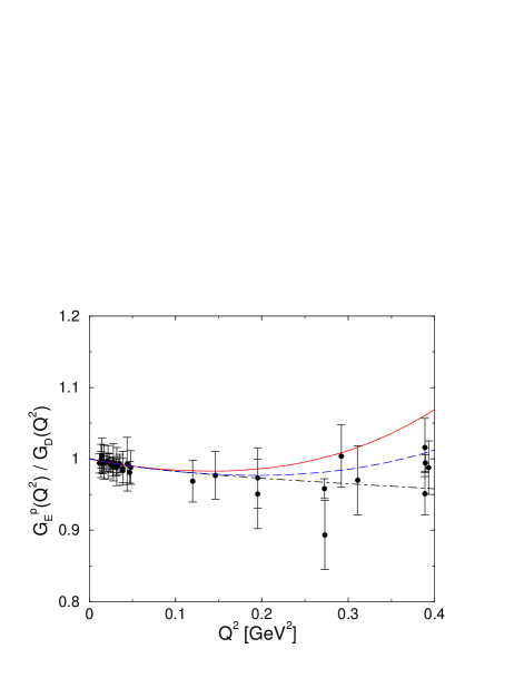
Figure 2: The proton electric form factor in SU(3) (red/full curve) and SU(2) (blue/dashed curve) relativistic baryon chiral perturbation theory including vector mesons, divided by the dipole form factor. For comparison, we show the dispersion theoretical result (black dot–dashed curve) and the world data available in this energy range.

 

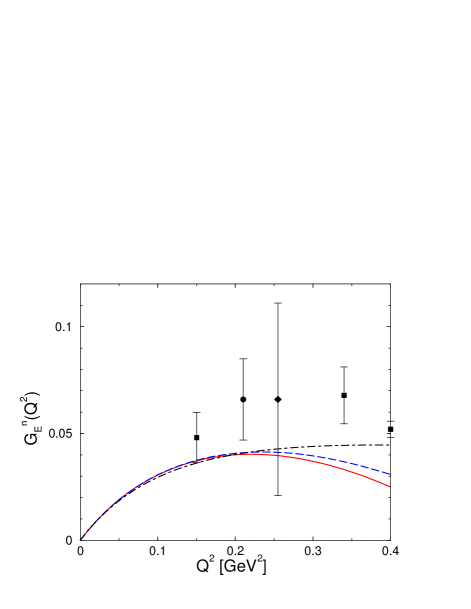
Figure 3: The neutron electric form factor in SU(3) (red/full curve) and SU(2) (blue/dashed curve) relativistic baryon chiral perturbation theory including vector mesons. Also given is the result of the dispersion theoretical analysis (black dot–dashed curve). We only show the more recent data as given in [28].

 

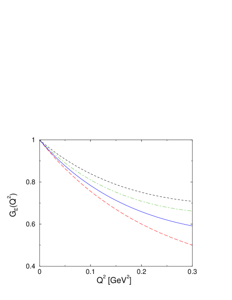
Figure 4: Predictions for the electric form factors of the charged hyperons $\Sigma^{+}$ (green/dot–dashed line), $\Sigma^{-}$ (blue/full line), and $\Xi^{-}$ (black/dashed line). For the latter two, the absolute value of $G_{E}(Q^{2})$ is shown. For comparison, we also show the proton electric form factor (red/long–dashed line).

 

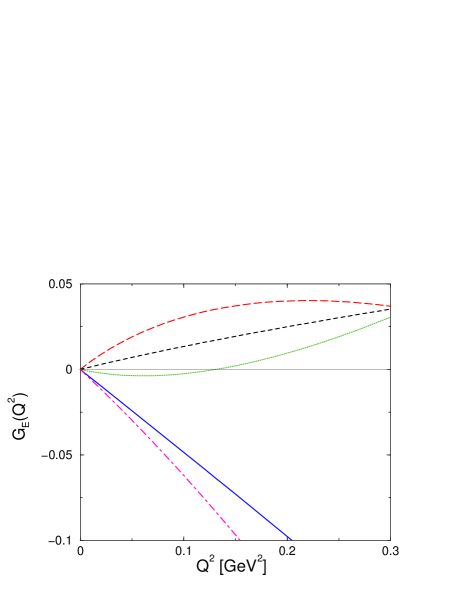
Figure 5: Predictions for the electric form factors of the neutral hyperons $\Lambda$ (blue/full line), $\Sigma^{0}$ (black/dashed line), $\Xi^{0}$ (pink/dot–dashed line), as well as the $\Lambda$–$\Sigma^{0}$ transition form factor (green/dotted line). For comparison, we also show the neutron electric form factor (red/long–dashed line).

 

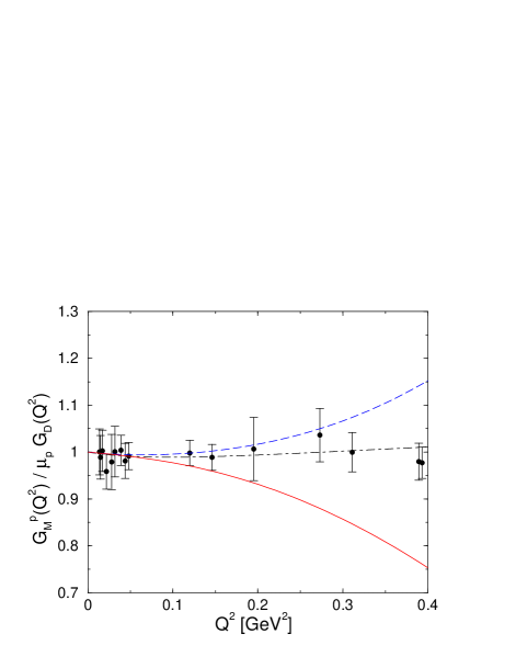
Figure 6: The proton magnetic form factor in SU(3) (red/full curve) and SU(2) (blue/dashed curve) relativistic baryon chiral perturbation theory including vector mesons, divided by the dipole form factor. For comparison, we show the dispersion theoretical result (black dot–dashed curve) and the world data available in this energy range.

 

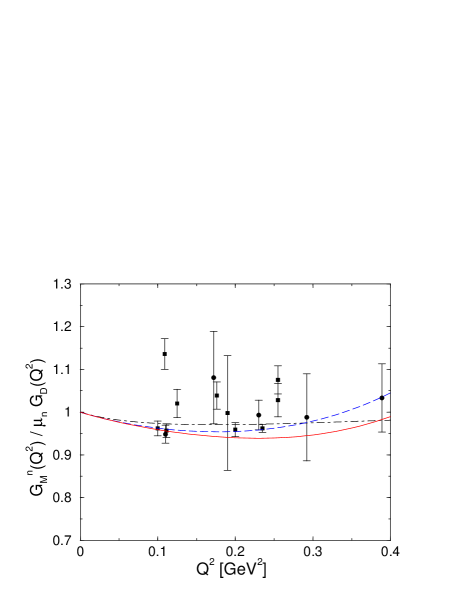
Figure 7: The neutron magnetic form factor in SU(3) (red/full curve) and SU(2) (blue/dashed curve) relativistic baryon chiral perturbation theory including vector mesons, divided by the dipole form factor. For comparison, we show the dispersion theoretical result (black dot–dashed curve) and the world data available in this energy range, where the data points denoted by squares (instead of circles) refer to the more recent measurements [29]. The older data can be traced back from [23].

References

- [1] G.G. Petratos, Nucl. Phys. A666&667 (2000) 61c.
- [2] B. Kubis and U.-G. Meißner, hep-ph/0007056, to be published in Nucl. Phys. A.
- [3] T. Becher and H. Leutwyler, Eur. Phys. J. C9 (1999) 643.
- [4] M. Adamovich et al., Eur. Phys. J. C8 (1999) 59.
- [5] I. Eschrich et al., hep-ex/9811003.
- [6] B. Kubis, T.R. Hemmert, and U.-G. Meißner, Phys. Lett. B456 (1999) 240.
- [7] S.J. Puglia, M.J. Ramsey-Musolf, and Shi-Lin Zhu, hep-ph/0008140.
- [8] E. Jenkins, M. Luke, A.V. Manohar, and M.J. Savage, Phys. Lett. B302 (1993) 482; (E) Phys. Lett. B388 (1996) 866.
- [9] U.-G. Meißner and S. Steininger, Nucl. Phys. B499 (1997) 349.
- [10] L. Durand and P. Ha, Phys. Rev. D58 (1998) 013010.
- [11] J. Kambor and M. Mojžiš, Phys. Lett. B476 (2000) 344.
- [12] S.J. Puglia and M.J. Ramsey-Musolf, Phys. Rev. D62 (2000) 034010.
- [13] D.B. Leinweber, R.M. Woloshyn, and T. Draper, Phys. Rev. D43 (1991) 1659.
- [14] B. Kubis, Thesis, Bonn University, in preparation.
- [15] J. Gasser and H. Leutwyler, Nucl. Phys. B250 (1985) 465.
- [16] N.H. Fuchs, M. Knecht, and J. Stern, Phys. Rev. D62 (2000) 033003.
- [17] P.G. Ratcliffe, Phys. Rev. D59 (1999) 014038.
- [18] V. Bernard, N. Kaiser, and U.-G. Meißner, Nucl. Phys. A615 (1997) 483.
- [19] N. Fettes, U.-G. Meißner, and S. Steininger, Nucl. Phys. A640 (1998) 199.
- [20] P. Büttiker and U.-G. Meißner, Nucl. Phys. A668 (2000) 97.
- [21] V. Bernard, N. Kaiser, and U.-G. Meißner, Nucl. Phys. B457 (1995) 147.
- [22] V. Bernard, H.W. Fearing, T.R. Hemmert, and U.-G. Meißner, Nucl. Phys. A635 (1998) 121; (E) Nucl. Phys. A642 (1998) 563.
- [23] P. Mergell, U.-G. Meißner, and D. Drechsel, Nucl. Phys. A596 (1996) 367.
- [24] H.-W. Hammer, U.-G. Meißner, and D. Drechsel, Phys. Lett. B385 (1996) 343.
- [25] M.J. Ramsey-Musolf and H. Ito, Phys. Rev. C55 (1997) 3066.
- [26] T.R. Hemmert, U.-G. Meißner, and S. Steininger, Phys. Lett. B437 (1998) 184.
- [27] T.R. Hemmert, B. Kubis, and U.-G. Meißner, Phys. Rev. C60 (1999) 045501.
- [28] T. Eden et al., Phys. Rev. C50 (1994) R1749; M. Meyerhoff et al., Phys. Lett. B327 (1994) 201; C. Herberg et al., Eur. Phys. J. A5 (1999) 131; I. Passchier et al., Phys. Rev. Lett. 82 (1999) 4988; M. Ostrick et al., Phys. Rev. Lett. 83 (1999) 276; J. Becker et al., Eur. Phys. J. A6 (1999) 329.
- [29] P. Markowitz et al., Phys. Rev. C48 (1993) R5; H. Gao et al., Phys. Rev. C50 (1994) R546; H. Anklin et al., Phys. Lett. B336 (1994) 313; E.E.W. Bruins et al., Phys. Rev. Lett. 75 (1995) 21; H. Anklin et al., Phys. Lett. B428 (1998) 248; W. Xu et al., Phys. Rev. Lett. 85 (2000) 2900.