Inflationary Initial Conditions Consistent with Causality

Abstract

The initial condition problem of inflation is examined from the perspective of both spacetime embedding and scalar field dynamics. The spacetime embedding problem is solved for arbitrary initial spatial curvature $\Omega$, which generalizes previous works that primarily treat the flat case $\Omega=1$. Scalar field dynamics that is consistent with the embedding constraints are examined, with the additional treatment of damping effects. The effects of inhomogeneities on the embedding problem also are considered. A category of initial conditions are identified that are not acausal and can develop into an inflationary regime.

PACS numbers: 98.80.Cq, 04.20.Gz, 98.80.Bp

In press Physical Review D 2001.

hep-ph/0010280.

I Introduction

Inflation is the foremost idea for explaining the large scale homogeneity and near flatness of the universe, which are the two main unexplained observational features in the standard hot big-bang model. The large scale homogeneity or horizon problem amounts to the fact that under hot big-bang evolution, due to a decelerating scale factor ${\ddot{a}}<0$, sufficiently separated regions of the present day observable universe would never have been in causal contact. Nevertheless, it appears the universe we observe looks very much the same, and in particular very smooth, in all directions. This fact is best seen in the cosmic microwave background radiation (CMB) which has temperature fluctuations of only one part in $10^{5}$ when measured from any direction in the sky [1].

The inflation solution to this horizon problem is to picture the universe during an early epoch to undergo an accelerated expansion, ${\ddot{a}}>0$. Such expansion can take an initially small causally connected patch and enlarge it to a size that comfortably encompasses our present day observed universe, thereby solving the horizon problem. To realize inflation, the equation of state within the inflationary patch must be of a very special form, possessing negative pressure. The potential energy of a scalar field has an equation of state that satisfies this requirement. This fact has been a key link towards a dynamical realization of inflation and thereby has further motivated the inflation solution.

As inflation is meant to solve the horizon problem, it is important that it does not require acausal initial conditions. In particular, the picture of inflation considered here is for the universe to emerge from an initial singularity and then enter into a hot big-bang radiation dominated evolution. At some time $t_{i}$ after the initial singularity, the conditions appropriate for inflation should occur within a small patch that is contained within the causal horizon at that time. Chaotic inflation [2, 3] does not fall into this picture as there inflation is thought to start at the Planck epoch with homogeneity assumed on the Planck scale. To realize the picture of a “local” inflation, two requirements must be satisfied. First a physically sensible embedding must be demonstrated of the inflating patch immersed within a non-inflating background [4, 5, 6]. By embedding we mean matching the inflationary space time with the background space time at the boundary of the patch. Second, it must be shown that for $t>t_{i}$, the patch is dynamically stable to sustain inflation [7, 8, 9, 10, 11, 12, 13]. For example, large fluctuations, which conceivably could enter the inflating patch at a maximum rate limited only by causality, should not destroy the inflationary conditions within the patch.

Recently, a convenient methodology has been developed in [5, 6] for analyzing the embedding problem, based on the null Raychaudhuri equation [14, 15]. In Sec. II the flat spacetime ($\Omega=1$) formulation in [5] is generalized to arbitrary spacetime curvature. Then, an alternative solution from [5] to the embedding problem will be identified, which is especially attractive for an inflating patch with an open geometry. In Sec. III, initial conditions for scalar field dynamics are presented, which are consistent with causality and our embedding solution and which evolve into successful supercooled or warm inflationary regimes. In Sec. IV we combine the results in Sec. II and Sec. III to evaluate the effect of inhomogeneities on the embedding problem. Finally, Sec. V presents our conclusions.

II Embedding Conditions

The embedding of an inflationary patch within a background space time generally is regarded as unacceptable if there are any negative energy regions. This requirement often is referred to as the weak energy condition. The null Raychaudhuri equation is a useful diagnostic tool for determining the validity of this condition. This equation determines the evolution of the divergence $\theta\equiv\nabla^{\alpha}N_{\alpha}$ of the null ray vector $N^{\alpha}$ in a spacetime with an arbitrary, and not necessarily homogeneous, energy density distribution. In order for the weak energy condition to be valid, this equation implies that for a null geodesic the condition [5, 15]

$$\frac{d\theta}{ds}\leq 0$$ (1)

must be satisfied, where $s$ is an affine parameter along the null geodesic.

For application of Eq. (1) to the inflation embedding problem, the concept of anti-trapped and normal regions should be understood. Consider a sphere centered on a comoving observer. If the space time were not expanding, photons emitted from the surface of the sphere, radially towards the observer, would converge at the observer. However, the expansion tends to work against the bundle of rays converging to a point. If the expansion is rapid enough, the bundle of rays will have diverging trajectories and then the spherical surface from which the rays originated is said to be an anti-trapped surface [15]. The spherical surface with a radius $x_{\rm mas}$ is known as the minimally anti-trapped surface (MAS) if any sphere with a larger radius is anti-trapped. For inwardly directed null rays, the divergence, $\theta$, will be positive in anti-trapped regions of space. On the other hand, if $\theta$ is negative for inwardly directed null rays and positive for outwardly directed null rays, the region is called normal.

These definitions are convenient when analyzing the weak energy condition based on Eq. (1). For example, one can immediately conclude [5] that if an outer normal region bounds an inner anti-trapped region in a not necessarily homogeneous, spherically symmetric space time, the weak energy condition would be violated, thus implying negative energy is required at the boundary of such a configuration.

For the inflation problem, the inner region is modeled as the putative inflation patch (INF) and it is immersed within a outer background (BG) expanding spacetime region. As a first approximation, both the INF and BG regions are characterized by FRW metrics of the form

$$ds^{2}=-dt^{2}+a^{2}\left(\frac{dr^{2}}{1-\kappa r^{2}}+r^{2}d\Omega^{2}\right),$$ (2)

where $\kappa=-1$ for an open geometry, 0 for a flat geometry and 1 for a closed geometry. The effect of inhomogeneities in the BG will be considered in Sec. IV. The INF patch should be homogeneous. In what follows, $\theta$ and $x_{\rm mas}$ will be computed for a spacetime characterized by the metric Eq. (2). The results below are applicable for both the INF and BG regions, given that the appropriate parameters are used in Eq. (2) for the two different spacetime regions.

Proceeding with this calculation, the determinant of the metric Eq. (2) is

$$g=|\mbox{det}(g_{\mu\nu})|=a^{6}r^{4}(1-\kappa r^{2})^{-1}\sin^{2}\psi,$$ (3)

where $\psi$ is the polar angle. An incoming light ray (null vector) is given by

$$N^{\alpha}=\frac{1}{a}\left[\delta^{\alpha}_{0}-a^{-1}(1-\kappa r^{2})^{1/2}\delta^{\alpha}_{1}\right],$$ (4)

with the divergence of the null rays being

$$\theta=\frac{1}{\sqrt{g}}(\sqrt{g}N^{\alpha})_{,\alpha}.$$ (5)

Substituting equations (3) and (4) into (5) gives

$$\theta=\frac{2}{a}\left({\rm H}-\frac{(1-\kappa r^{2})^{1/2}}{ar}\right)$$ (6)

with ${\rm H}\equiv{\dot{a}}/a$ the Hubble parameter. The above recovers equation (10) of [5] for $\kappa=0$.

The physical distance is given by

$$x = a\int dr(1-\kappa r^{2})^{-1/2}$$ (7)

$$= a\,\mbox{arcsinh(r)},\quad\mbox{for $\kappa=-1$}$$ (8)

The MAS comoving distance, $r_{\rm mas}$, must give a zero divergence and so from Eq. (6) with, for example, $\kappa=-1$

$${\rm H}-\frac{{(1+\mbox{$r_{\rm mas}$}^{2})}^{1/2}}{a\mbox{$r_{\rm mas}$}}=0,$$ (9)

from which we get, using equation (8),

$$\mbox{$x_{\rm mas}$}=a\,\mbox{arcsinh}\left[({\rm H}^{2}a^{2}-1)^{-1/2}\right].$$ (10)

From the Friedman equation:

$${\rm H}^{2}a^{2}=\frac{\kappa}{\Omega-1}$$ (11)

Substituting (11) into (10) gives the solution for $x_{\rm mas}$ as a function of $\Omega<1$. A similar equation can be derived for the closed case $(1<\Omega<2)$ where an upper limit is needed on $\Omega$ to ensure that $1/{\rm H}$ is smaller than the radius of the Universe. Therefore, the general MAS size is given by

$$\mbox{$x_{\rm mas}$}(t)=\frac{1}{\rm H}\left\{\begin{array}[]{ll}\frac{1}{(1-\Omega)^{1/2}}\mbox{arcsinh}\left(\sqrt{\frac{1-\Omega}{\Omega}}\right),&0<\Omega<1\\ 1,&\Omega=1\\ \frac{1}{(\Omega-1)^{1/2}}\mbox{arcsin}\left(\sqrt{\frac{\Omega-1}{\Omega}}\right),&1<\Omega<2\end{array}\right.$$ (12)

FIG. 1.: A plot of MAS size as function of the density.

A plot of equation (12) is given in Fig. 1. As can be seen, the size of the MAS becomes arbitrarily large relative to the Hubble radius as $\Omega\rightarrow 0$.

The results for the $x_{\rm mas}$ derived above are valid for either the INF or BG region. In [5], the case $\Omega=1$ was treated, and our calculation above is consistent with them in this limit. Before proceeding with our analysis for general $\Omega$, let us review the results of [5] for $\Omega=1$. The background spacetime in their work is pictured, as for us, as evolving in a hot big bang regime. For $\Omega=1$ and standard forms of matter, e.g. radiation, non-relativitic matter, etc…, the Hubble horizon sets the the scale on which causal processes can take place. For definiteness, if we take the background causal horizon size as $\mbox{$x_{\rm p}^{\rm bg}$}=1/\mbox{${\rm H}_{\rm bg}$}$, then by Eq. (12) for $\Omega=1$, $\mbox{$x_{\rm p}^{\rm bg}$}=\mbox{$x_{\rm mas}^{\rm bg}$}$.

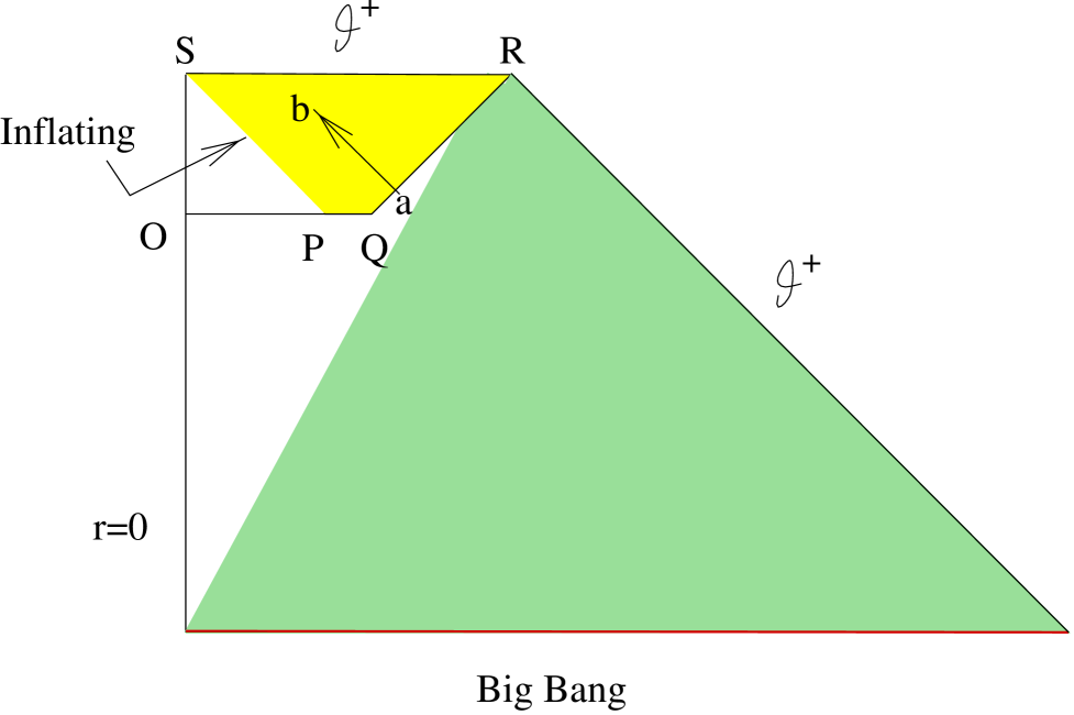
FIG. 2.: A Penrose diagram for local inflation (adapted from [5] ). The arrow (ab) denotes a radially directed null-geodesic going from the normal background space time to the anti-trapped space time inside the patch. Shading represents anti-trapped regions.

Fig. 2 shows a Penrose diagram for an embedding that violates the weak energy condition. Here, at the beginning of inflation, $x_{\rm p}^{\rm inf}$ is represented by line OQ and $x_{\rm mas}^{\rm inf}$ is represented by line OP. An inflating patch is pictured to develop within some region inside the background (polygon OQRS in Fig. 2). In the inflationary patch, they assume a different Hubble parameter ${\rm H}_{\rm inf}$ and assume the size of this patch must be $\mbox{$x_{\rm p}^{\rm inf}$}>1/\mbox{${\rm H}_{\rm inf}$}$. This assumption can be justified by requiring the patch to be stable against perturbations and will be discussed further in the next section. By Eq. (12) it also implies $\mbox{$x_{\rm mas}^{\rm inf}$}=1/\mbox{${\rm H}_{\rm inf}$}$ for $\Omega=1$. If the patch is to be set up by causal processes then we would expect it to be smaller than the background Hubble horizon, $\mbox{$x_{\rm p}^{\rm inf}$}<\mbox{$1/{\rm H}_{\rm bg}$}$. These conditions combined imply $\mbox{$x_{\rm mas}^{\rm bg}$}=\mbox{$1/{\rm H}_{\rm bg}$}>\mbox{$x_{\rm p}^{\rm inf}$}>\mbox{$x_{\rm mas}^{\rm inf}$}$. As such the region between $x_{\rm mas}^{\rm bg}$ and $x_{\rm p}^{\rm inf}$ is normal with respect to the BG-region and the region between $x_{\rm p}^{\rm inf}$ and $x_{\rm mas}^{\rm inf}$ is anti-trapped with respect to the inflating patch. Thus an in-going null ray will go from a negative divergence region to a positive divergence region. Based on Eq. (1) this leads to a violation of the weak energy condition. Due to this fact, in [5] they conclude that the only way to avoid this violation is to have $\mbox{$x_{\rm p}^{\rm inf}$}>\mbox{$1/{\rm H}_{\rm bg}$}$ which may be impossible or at least very difficult to come about through causal processes.

Although this analysis assumed a homogeneous background, the general result of [5] was that if the inflationary patch contained a MAS then it must be larger than the background MAS. One of the main aims of this article is to further examine the implications this has for a causal embedding of an inflationary patch.

Our first observation is that there is an embedding consistent with both causality and the weak energy condition, in particular

$$\mbox{$x_{\rm p}^{\rm bg}$},\mbox{$x_{\rm mas}^{\rm inf}$}>\mbox{$x_{\rm p}^{\rm inf}$}\,.$$ (13)

Since $x_{\rm p}^{\rm inf}$ in Eq. (13) is smaller than $x_{\rm p}^{\rm bg}$, it implies consistency with causality. A region which is smaller than its MAS will have no anti-trapped surfaces. Thus in our proposed embedding Eq. (13), the INF-BG boundary is between two normal regions. As such, provided $\mbox{$\theta^{\rm inf}$}]_{\rm boundary}$ is sufficiently smaller than $\mbox{$\theta^{\rm bg}$}]_{\rm boundary}$, the weak energy condition is satisfied. One interesting feature of the embedding Eq. (13) is that for $\mbox{$\Omega_{\rm inf}$}<1$ it is acceptable for $\mbox{$x_{\rm p}^{\rm inf}$}>1/{\rm H}_{\rm inf}$.

As inflation proceeds, $\mbox{$\Omega_{\rm inf}$}\rightarrow 1$ and so $\mbox{$x_{\rm mas}^{\rm inf}$}\rightarrow\mbox{$1/{\rm H}_{\rm inf}$}$. One of the main features of inflation is that modes of a matter perturbation become larger than the Hubble radius as the Universe expands. It follows that eventually $\mbox{$x_{\rm p}^{\rm inf}$}>\mbox{$1/{\rm H}_{\rm inf}$},\mbox{$x_{\rm mas}^{\rm inf}$}$ will need to occur. This will not cause violation of the weak energy condition provided that $\mbox{$x_{\rm p}^{\rm inf}$}>\mbox{$x_{\rm mas}^{\rm bg}$}$ at that time.

Fig. 3 shows a Penrose diagram of the proposed embedding. At point T in the figure, $\mbox{$x_{\rm p}^{\rm inf}$}=\mbox{$x_{\rm mas}^{\rm bg}$}$ and at point P, $\mbox{$x_{\rm p}^{\rm inf}$}=\mbox{$x_{\rm mas}^{\rm inf}$}$.

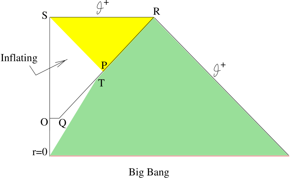
FIG. 3.: A Penrose diagram for local inflation with an embedding that does not violate the weak energy condition and is not acausal.

As can be seen the anti-trapped region develops in the patch only after the patch has become greater than the background MAS.

There is another embedding which does not violate the weak energy condition, in this case for $\mbox{$\Omega_{\rm bg}$}>1$, but it proves not to be as useful,

$$\mbox{$x_{\rm mas}^{\rm inf}$},\mbox{$x_{\rm mas}^{\rm bg}$}<\mbox{$x_{\rm p}^{\rm inf}$}<\mbox{$1/{\rm H}_{\rm bg}$}\,.$$ (14)

This solution is restricted by the upper limit on $\Omega_{\rm bg}$ that gives a lower limit (from Eq. 12) of $\mbox{$x_{\rm mas}^{\rm bg}$}\approx 0.8/\mbox{${\rm H}_{\rm bg}$}$ for $\Omega=2$. As the causal scale $x_{\rm p}^{\rm bg}$ can be only of the order of $1/{\rm H}_{\rm bg}$, such a large inflationary patch may still be acausal.

Additional information about embedding constraints can be obtained through the Israel junction conditions [16]. In [17, 18] conditions were derived for the embedding of one FRW spacetime within another. The Israel junction conditions require the extrinsic curvature on the background side of the boundary to be smaller than the extrinsic curvature on the patch side of the boundary if the boundary surface energy density is to be positive. It can then be shown [17, 18] that if the energy density of the background $\rho_{\rm bg}$ is greater than that of the patch $\rho_{\rm inf}$, the Israel junction conditions can be satisfied for an inflationary patch of arbitrary size and geometry with any background geometry. They also show for $\mbox{$\rho_{\rm bg}$}<\mbox{$\rho_{\rm inf}$}$, an embedding consistent with the Israel junction conditions and $\mbox{$x_{\rm p}^{\rm inf}$}<\mbox{$1/{\rm H}_{\rm bg}$}$ requires the background geometry to be closed with the geometry of the inflationary patch arbitrary.

III Dynamic Conditions

An immediate concern with the proposed embedding Eq. (13) regards the size of the inflationary patch. As far as the embedding conditions are concerned, the patch size simply must lie below the $x_{\rm mas}$ line in Fig. 1. In particular, for $\mbox{$\Omega_{\rm inf}$}>1$ the inflationary patch size must be $<1/\mbox{${\rm H}_{\rm inf}$}$. However, for $\mbox{$\Omega_{\rm inf}$}<1$, the inflationary patch size can be $>1/\mbox{${\rm H}_{\rm inf}$}$. The primary question which remains is what the minimal initial inflation patch size can be in order to be dynamically stable for inflation to commence. For example, if the initial patch is too small, then large fluctuations initially outside the patch could enter inside at a rate sufficiently fast to destroy the inflationary conditions. In this section, the dynamic conditions necessary for inflation will be examined for both the scalar field and a background radiation component.

A Scalar Field

For scalar field driven inflation, the general dynamical conditions necessary for a finite spatial patch to initiate and sustain inflation have been considered in [7, 8, 9, 10, 11, 12] and a comprehensive review has been given in [13]. Here the requirements addressed in these works, primarily the review [13], will be systematically examined with emphasis on determining their implications for the minimal initial inflationary patch size. Our considerations of scalar field dynamics will generalize those in the above stated works, which focused on supercooled inflationary dynamics [19, 20, 2], in that here warm inflation dynamics [21] also will be treated.

The classical evolution equation for the scalar inflaton field has the general form

$${\ddot{\phi}}({\bf x},t)+[3{\rm H}+\Gamma]{\dot{\phi}}({\bf x},t)$$ (15)

$$- a^{-2}\nabla^{2}\phi({\bf x},t)+\frac{\delta V(\phi)}{\delta\phi({\bf x},t)}=0,$$ (16)

where $\Gamma$ is a dissipative coefficient, which represents the effective interaction of the inflaton with other fields. Here and below $\phi({\bf x},t)$ is a classical real number which contains the ensemble average of the quantum and/or thermal fluctuations. In supercooled inflation, it is assumed the inflaton is isolated, in which case $\Gamma=0$. Thus no radiation is produced during inflation and the universe inflates in a supercooled state. On the other hand, in warm inflation the inflaton interacts with other fields, and the $\Gamma{\dot{\phi}}$ term is the simplest representation of their effect on the evolution of the inflaton, with generally $\Gamma>{\rm H}$. Due to these interactions, radiation is dissipated from the inflaton system into the universe throughout the inflation period. In general, $\Gamma$ can vary as a function of the inflaton field mode to which it is associated, but here $\Gamma$ is treated as a constant.

There are two types of potential $V(\phi)$ in Eq. (16) that typically are treated in inflationary cosmology, a purely concave potential of the generic form $V\sim m^{2}\phi^{2}+\lambda\phi^{4}$ and a double well potential such as $V\sim(\phi^{2}-m^{2})^{2}$. Our discussion to follow will focus of the former type of potential and at the end we will comment on the case of the double well potential. Furthermore, for most of our discussion it will be adequate to consider the simplest case of a quadratic potential, $V=\frac{1}{2}m^{2}\phi^{2}$. In this case, going to Fourier space where we put the universe in a box

$$\phi({\bf x},t)=\sum_{\bf k}\phi_{\bf k}(t)e^{i{\bf k}\cdot{\bf x}},$$ (17)

Eq. (16) becomes,

$${\ddot{\phi}}_{\bf k}+[3{\rm H}+\Gamma]{\dot{\phi}}_{\bf k}(t)+a^{-2}k^{2}\phi_{\bf k}(t)+m^{2}\phi_{\bf k}(t)=0,$$ (18)

where $k^{2}\equiv|{\bf k}|^{2}$ with ${\bf k}$ the comoving wave-vector and ${\bf k}/a(t)$ the corresponding physical wave-vector at time $t$.

A necessary condition for inflation is that the zero mode $\phi_{{\bf k}=0}$, must have a sufficiently large and long-sustained amplitude so that the potential energy $V=\frac{1}{2}m^{2}\phi_{0}^{2}$ dominates the equation of state of the universe, thereby driving inflation. This leads to the familiar slow-roll conditions, which require the curvature of the potential to be sufficiently flat so that Eq. (18) for the zero mode becomes first order in time

$${\dot{\phi}}_{0}=-\frac{dV(\phi)/d\phi_{0}}{3{\rm H}+\Gamma}.$$ (19)

The dynamic initial condition problem is that the above requirements should not be too special and in particular should not violate causality. The most acute initial condition problem discussed in [13] and related works is that generally the initial inflaton field configuration will be very inhomogeneous, thus considerable contribution of gradient energy ($(\nabla\phi)^{2}$) should be present. In its own right, the gradient term for comoving mode ${\bf k}$ has energy density $\rho_{\nabla}=({\bf k}^{2}/2a^{2})\phi_{\bf k}^{2}$ and equation of state $p_{\nabla}=-\rho_{\nabla}/3$. From the scale factor equation

$$\frac{\ddot{a}}{a}=-\frac{4\pi G}{3}(\rho+3p),$$ (20)

the effect of the gradient energy vanishes on the right hand side. As such, any additional contribution from vacuum energy still should drive inflation. However, excited modes with $k/a>3{\rm H}+\Gamma$ not only will possess gradient energy, but based on Eq. (18) are under-damped. As such, they also have a kinetic energy contribution $\rho_{\dot{\phi}}\sim{\dot{\phi}}^{2}_{\bf k}$, which has an equation of state $p_{\dot{\phi}}=\rho_{\dot{\phi}}$. If the kinetic energy components of these modes dominates the energy density in the universe, then from Eq. (20) inflation will cease to occur.

For the case of supercooled inflation, since $\Gamma=0$, the simplest way to avoid this problem is to require that modes with $k/a\gtrsim{\rm H}$ initially should not be excited. In other words, the inflaton field initially should be smooth up to physical scales larger than $\sim 1/{\rm H}$. However, under general conditions, the causal size of the pre-inflation patch also will be of order the Hubble radius $1/{\rm H}$. As such this homogeneity requirement on the initial inflaton field impinges on being acausal, since this condition essentially requires initially smooth conditions up to the causal scale.

To treat excited modes with $k/a>{\rm H}$ in the supercooled inflation case, the initial condition dynamics are much more complicated. A simple analytical method applied to this situation is the effective density approximation presented in [7, 11] and reviewed in Sec. 7.2 of [13]. In this approach, the inhomogeneities of the inflaton are treated in determining its evolution, but the effect of these inhomogeneities on the metric is only treated in the Friedmann equation through homogeneous terms that represent the effective gradient and kinetic energy densities as

$$\left(\frac{\dot{a}}{a}\right)^{2}\equiv{\rm H}^{2}=\frac{8\pi G}{3}\left[\frac{1}{2}{\dot{\phi}}_{0}^{2}+\frac{1}{2}m^{2}\phi_{0}^{2}\right.+$$ (21)

$$\left.\frac{1}{2}\sum_{\bf k}[{\dot{\phi}}_{\bf k}^{2}+(\frac{{\bf k}^{2}}{a^{2}}+m^{2})\phi_{\bf k}^{2}]+\rho_{r}\right]-\frac{\kappa}{a^{2}}.$$ (22)

For initial field configurations with sufficiently excited $k/a>{\rm H}$ modes so that their gradient energies dominate the equation of state of the universe, the effective density approximation indicates the Friedmann and inflaton evolution equations are highly coupled. In particular, the Hubble parameter will be dominated by the gradient energy term and this will act back on the inflaton evolution through the $3{\rm H}{\dot{\phi}}$ term. Furthermore, the initially large gradient terms also can in turn induce large kinetic energy in the modes. The outcome found in [7, 11, 13] (see also [9]) for this case is that the universe expansion is non-inflationary. On the other hand, for the excited $k/a>{\rm H}$ modes with smaller amplitudes, their evolution will be oscillatory and once again the universe expansion is non-inflationary. For either of these two possibilities, this approximation method finds that after an initial period of detaining the universe in a non-inflationary regime, the effect of these higher modes becomes negligible. At this point the remaining vacuum energy dominates and eventually inflation proceeds.

Numerical simulations [10, 11] which exactly treat the effects on the metric due to the inhomogeneities in the inflaton field, in fact, do not support this final conclusion of the effective density approximation. Instead, the simulations find that once modes with $k/a>{\rm H}$ are sufficiently excited, inflation generally does not occur or is highly suppressed. Although the final conclusion of the effective density approximation was incorrect, it at least indicated that there is nontrivial interplay between the inflaton and metric evolution equations once significant short distance inhomogeneities are present in the inflaton field.

In contrast to the supercooled case, once $\Gamma>{\rm H}$, the effective density approximation indicates that for modes with $\Gamma>k/a>{\rm H}$, there is almost no feedback between the inflaton and Friedmann equations. The evolution equation for these inflaton modes is

$$\Gamma\dot{\phi}_{\bf k}(t)=\left[\frac{{\bf k}^{2}}{a^{2}}+m^{2}\right]\phi_{\bf k}(t),$$ (23)

and in particular is independent of ${\rm H}$. This in turn implies all these modes are over-damped. As such, they only contribute gradient energy to the equation of state of the universe, which alone is ineffective in preventing inflation. Thus up to the predictions of the effective density approximation, in contrast to the supercooled case, in this warm inflation case modes with $k/a<\Gamma$ show little coupling between the inflaton and Friedmann equations. It is evident that dynamics with a $\Gamma{\dot{\phi}}$ damping term should have qualitative differences for the initial condition problem compared to the case with $\Gamma=0$. In particular, modes of physical wavelength smaller that the Hubble radius $1/{\rm H}$ but larger than $1/\Gamma$ could still be substantially excited without destroying entrance into inflation. This implies inflationary patch sizes smaller than the Hubble radius may be dynamically stable in sustaining inflation and based on the results of Sec. II, they also provide consistent spacetime embeddings, especially for $\mbox{$\Omega_{\rm inf}$}<1$. Furthermore, studies of warm inflation [21, 22, 23], including the first principles quantum field theory model [24], generally find that to obtain adequate inflationary e-folds, $N_{e}\stackrel{{\scriptstyle>}}{{\sim}}60$, it requires $\Gamma\approx N_{e}m^{2}/{\rm H}$ with $m\gtrsim{\rm H}$ so that $\Gamma\gtrsim N_{e}{\rm H}$ and thus $1/\Gamma\ll 1/{\rm H}$. As such, for warm inflationary conditions this simple analysis suggests that the smoothness requirement on the initial inflationary patch is at scales much smaller than the Hubble radius $1/{\rm H}$, which therefore imposes no violation of causality.

These considerations can be extended to the more complicated situation where the inflaton evolution equation has nonlinear terms, such as the $\phi^{4}$ interaction term. For supercooled inflation, the effect of such interactions has been considered from the perspective of mode mixing for some special cases in [8, 9] and through computer simulations of scalar fields in one spatial dimension in [10, 11]. Up to the scope of these works, their analysis concludes that nonlinear interactions do not present any additional complications to the initial condition problem. For the warm inflation case, this conclusion can be stated in more general terms. In particular, the dissipative coefficient $\Gamma$ completely damps the evolution, thus suppressing mode mixing, of all modes with $k/a<\Gamma$. As such, initially excited modes with $k/a<\Gamma$ will evolve independently within the time scales relevant to the initial period when inflation begins. The only effect of excited modes with $k/a<\Gamma$ is to contribute gradient energy to the equation of state of the universe, and this alone is ineffective in suppressing inflation. Therefore, provided the inflaton field also initially maintains some vacuum energy, no aspect of the inflaton’s dynamics in the early period acts to circumvent entrance into the inflation phase.

Although the above discussion addressed the main impediment in scalar field dynamics that can prevent inflation, there are a few smaller concerns worth mentioning here. One detail treated in [13] is inflaton initial conditions with large kinetic energy. For $\Gamma=0$, it is shown in [13] that this problem is self-correcting, and so should not pose a major barrier in entering into the inflation phase. For $\Gamma>{\rm H}$, the severity of this problem diminishes further since this damping term is an additional effect that helps suppress the initial kinetic energy. Another secondary detail is that above we only treated concave potentials. For double well potentials, $V\sim(\phi^{2}-m^{2})^{2}$, as in the case of new inflation [20], inflation requires the field to be well localized at the top of the potential hill $\phi=0$ and almost at rest. These requirements are necessary, otherwise as found in various studies [25], the field can easily break up into several small domains with randomly varying signs of the amplitude. For the supercooled case, new inflation, the basic conclusion about the initial conditions required for inflation has been that they are not very robust [25, 26, 13]. The inclusion of a dissipative term $\Gamma>{\rm H}$ will not necessarily improve this situation. On the one hand, such a term helps considerably to damp kinetic energy, thus allowing the inflaton to remain at the top of the hill longer and drive inflation. On the other hand, if such a damping term arises too early before inflation is to begin, since it freezes the evolution of excited inflaton modes, it could prevent the initial inflaton field configuration from equilibriating to $\phi=0$.

Finally in the above discussion $\Gamma\neq 0$ generally represented warm inflation dynamics, although even for supercooled inflation, if radiation is present at the onset of inflation, such as in the new [20] and thermal [27] inflation pictures, the effective evolution of the inflaton could have a damping term of the form $\Gamma{\dot{\phi}}$. Since our focus is on the initial phase at the onset of inflation, it is possible the effect of such damping terms also may be applicable to the initial condition problem in some supercooled inflation models.

B Radiation Component

So far we only considered the inflaton field system, but in addition the universe could possess some background component of radiation energy density, $\rho^{\rm bg}_{\rm r}$. To realize inflation, minimally it requires the vacuum energy density $\rho_{\rm v}$ to dominate in the patch, $\mbox{$\rho^{\rm bg}_{\rm r}$}<\rho_{\rm v}$. If initially $\rho^{\rm bg}_{\rm r}$ is larger than $\rho_{\rm v}$, expansion of the universe will red-shift the radiation. Thus provided the vacuum energy sustains itself during this early period, inflation eventually will start. This is the standard new and warm inflation pictures.

One could imagine that in some small patch inside a larger causally created spatial region, the inflaton field configuration is reasonably smooth and is sustaining a sizable vacuum energy of magnitude

$$\rho_{\rm v}\approx\mbox{$\rho^{\rm bg}_{\rm r}$}.$$ (24)

As the universe expands $\rho^{\rm bg}_{\rm r}$ decreases and provided $\rho_{\rm v}$ sustains itself, inflation will begin in the patch. However at this moment, there could be large energy fluctuations in the radiation bath or other fields that are just outside the putative inflationary patch. One would like to understand how probable it is for such a situation to curtail the inflation that had started in the patch.

To answer this question based solely on causality considerations, one should consider the case of a perturbation starting on the patch boundary and moving across the patch at the speed of light, and make the extreme assumption that as the perturbation overruns regions of the inflation patch, those regions convert back to being non-inflating. The question is what minimal initial inflationary patch size is needed so that its expansion under inflation is faster than its contraction due to the impinging perturbations. For the case of flat geometry $\Omega=1$, this question was addressed in [13] and they concluded that the patch size should be at least 3 times the Hubble radius in order for inflation to succeed in enlarging the patch. For a general $\Omega$, we can address this question by evaluating the maximum distance a perturbation can travel in the patch between the initial $t_{i}$ and final $t_{f}$ time of inflation

$$x_{\rm pert}=a(t)\int_{t_{i}}^{t_{f}}a^{-1}\,dt.$$ (25)

Note that since $a$ is growing rapidly, there is negligible error in taking $t_{f}\rightarrow\infty$ which implies $x_{\rm pert}$ essentially is the event horizon. We have examined Eq. (25) for a variety of supercooled and warm inflation models and generally find $x_{\rm pert}\approx\mbox{$x_{\rm mas}$}$.

Thus in the most ideal case, an inflationary patch smaller than the event horizon can not be stable. Here an important point of syntax should be noted, that the generic size here is the event horizon and not the Hubble radius, although for the flat case, $\Omega=1$, both are of the same order. The above is the ideal bound based on causality. However, realistic dynamics also must be considered.

One case which corresponds to external perturbations entering into an initially inflating patch is the case treated in Subsect. IIIA of the mixing of high wavenumber modes. For the inflaton field interacting with itself or with other fields, we argued above that if a dissipative term of the form $\Gamma{\dot{\phi}}$ is present in the inflaton effective evolution equation, then mode mixing up to wave-numbers $k/a<\Gamma$ will not occur within the time scale relevant to the initial condition problem.

In terms of the radiation bath, suppose a small vacuum dominated inflationary regime emerges, which is immersed inside a larger region containing radiation and gradient energy density. Since the inflationary patch has negative pressure, the surrounding radiation will flow into it. The degree to which the pressure differences are significant to this process depends on the magnitudes of the radiation, gradient and vacuum energies in both regions as well as detailed dynamical considerations[17, 28]. Nevertheless, suppose the radiation tries to become uniform over the entire region, including the patch. Since the patch started to inflate, it meant that initially $\rho_{\rm v}\gtrsim\mbox{$\rho^{\rm bg}_{\rm r}$}$. As time commences, provided $\rho_{\rm v}$ remains constant, since expansion of the background will decrease $\rho^{\rm bg}_{\rm r}$, it means the amount of radiation that flows into the inflationary patch will be less than $\rho_{\rm v}$. Thus irrespective of whether the inflaton dynamics is supercooled or warm, the patch should sustain a type of warm inflation due to this influx of radiation from the regions that surround it.

A thorough understanding of the initial condition dynamics in presence of a background radiation component is complicated. To our knowledge, no quantitative analysis has been done along these lines. The review [13] only illustrated the problem with the example quoted above Eq. (25) based on causality considerations but offered no dynamical examples with respect to a background radiation component. Here we have offered one scenario where the background radiation component should not prevent inflation from occurring. In particular, this example demonstrates that causality bounds on the rate at which radiation or other energy fluctuations enter the patch are not the only aspect of this problem. In addition, the magnitude of the entering radiation must be adequately large to overwhelm the vacuum energy. We have offered arguments above that indicate this latter requirement is not generic.

IV Dynamical Effects on Embedding

As discussed in Sec. II, a causally favourable embedding requires the inflationary patch to start smaller than the background MAS and then grow larger than it. A minimum condition for this to happen is that the particle horizon of the background eventually becomes greater than the background MAS.

For $p=\omega\rho$, the particle horizon is given by [29]

$$d(t)=\frac{1}{H}\int_{0}^{1}\frac{dx}{\left[x^{2}(1-\Omega(t))+\Omega(t)x^{1-3w}\right]^{1/2}}.$$ (26)

Comparing this equation with Eq. (12) it can be seen that the particle horizon will only become greater than the MAS if $\omega<1/3$. This condition was also noted in [30] from a slightly different perspective. There the patch was taken to start larger than the background MAS.

It follows that our proposed embedding will not work for a pure radiation background which has $\omega=1/3$. However, in general the background will consist of radiation and an inhomogeneous scalar field. As discussed in Sec. III, the gradient energy of the scalar field has $\omega=-1/3$ and the potential energy has $\omega=-1$ while the kinetic energy has $\omega=1$. It follows that if the background is gradient dominated our causal embedding scheme will be viable, whereas our scheme fails if the kinetic term dominates. However, the kinetic energy of the scalar field will be suppressed if the dissipative coefficient $\Gamma$ of Sec. III is sufficiently large. This is already required inside the putative inflation patch in order to realize inflation. Thus, it is not unreasonable to expect $\Gamma$ in the background region to be of the same magnitude.

V Conclusion

This paper has investigated the initial condition problem of inflation from the perspective both of spacetime embedding and inflaton dynamics. Our study has highlighted two attributes of this problem which have not been addressed in other works. First, from the perspective of spacetime embedding, we have observed that the global geometry can play an important role in determining the size of the initial inflationary patch that is consistent with the weak energy condition. Second, from the perspective of inflaton dynamics, we have noted that a $\Gamma{\dot{\phi}}$ damping term could alleviate several problems which traditionally have led to large scale homogeneity requirements before inflation.

The purpose of this paper was to note for both these attributes, their salient features with respect to the initial condition problem. In the wake of this, several details emerge that must be understood. Below, we will review the main result we found for both attributes and then discuss the questions that must be addressed in future work.

For a causally generated patch a successful embedding can be achieved if the patch does not contain an anti-trapped region. We have shown that the MAS size can be arbitrarily larger than the Hubble scale provided $\Omega$ is made small enough. So if the patch Hubble horizon is taken as the minimum stable patch size, then the patch does not have to contain an anti-trapped region if $\mbox{$\Omega_{\rm inf}$}<1$. This generalizes the analysis of [5] which was only for $\Omega=1$. However, without the effects of damping, it appears that the event horizon, not the Hubble horizon, is the minimum stable patch size. For the de Sitter case one can see analytically that the event horizon is equal to the MAS size regardless of $\Omega$ and numerical calculations suggest the same is true for power law inflation. However, radiation damping of perturbations could stabilize a patch smaller than the event horizon. In this case an open geometry for the patch would allow the patch not to contain an anti-trapped region and thus allow a causal embedding in an expanding background which does not violate the weak energy condition. Eventually the patch should develop a MAS within it, but by then it could have expanded to be larger than the background MAS.

For the dynamics problem, with respect to the scalar field the new consideration was the effect of a $\Gamma{\dot{\phi}}$ damping term. We found that such a term could suppress many of the effects from initial inhomogeneities of the inflaton, which in studies traditionally done without this term lead to important impediments to entering the inflation regime. It appears evident that inclusion of such a damping term will lead to qualitative differences in the initial condition problem. The most interesting outcome is initial inflationary patches smaller than the Hubble radius $1/{\rm H}$ may be able to inflate.

This paper examined the consequences of damping terms but did not delve into their fundamental origin. For the cosmological setting, such damping terms are typically associated with systems involving a scalar field interacting with fields of a radiation bath. In this case, such damping terms have been found in first principles calculations for certain warm inflation models [24], although more work is needed along these lines. It is worth noting here that in the early stages of certain supercooled inflaton scenarios where radiation is present, in particular new [20] and thermal [27] inflation, a careful examination of the dynamics may reveal damping terms similar to this. Since the initial stages are the crucial period for the initial condition problem, if further study supports the importance of such damping terms, it may be useful to better understand damping effects also in such scenarios.

Since the most suggestive situation for the damping terms is where in addition a radiation component is present in the universe, in Subsect. IIIB we also studied the effects of this component on the initial condition problem. Specifically we studied the case most suggestive for the initial stages of new and warm inflation, where a small inflation patch is submerged inside a larger radiation dominated spatial region. Our main observation has been that the minimal condition for the patch to inflate is that its vacuum energy density must be larger than the background radiation energy density. Provided the vacuum energy sustains itself, since expansion of the universe will dilute the radiation energy density, it is not clear-cut that the external radiation energy can act with sufficient magnitude to impede inflation inside the patch.

We have shown that the gradient terms, due to the inhomogeneous scalar field in the background space time, make it possible for the patch boundary to overtake the background MAS. However the kinetic energy of the scalar field must not be dominant for this to happen. This can be ensured by including a damping term in the scalar field equation.

VI Acknowledgements

We thank Robert Brandenberger, David Hochberg and Tanmay Vachaspati for helpful discussions. CG also would like to thank his colleagues in the Relativity and Cosmology Group for helpful discussions and in particular Roy Maartens for detailed comments and he acknowledges the support of an ORS award. AB acknowledges support of PPARC.

REFERENCES

- [1] C. L. Bennett et al., Astrophys. J. 464, L1 (1996).
- [2] A. Linde, Phys. Lett. 129B, 177 (1983).
- [3] A. Linde, “Particle Physics And Inflationary Cosmology,” Chur, Switzerland: Harwood (1990) (Contemporary concepts in physics, 5).
- [4] K. Sato, H. Kodama, M. Sasaki, and K. Maeda, Phys. Lett B108, 103 (1982); E. Fahri and A. Guth, Phys. Lett. B183, 149 (1987); S. Blau, E. Guendelman and A. Guth, Phys. Rev. D35, 1747 (1987); E. Fahri, A. Guth, and J. Guven, Nucl. Phys. B339, 417 (1990).
- [5] T. Vachaspati and M. Trodden, Phys. Rev. D61, 023502 (2000).
- [6] M. Trodden and T. Vachaspati, Mod. Phys. Lett. A14, 1661 (1999).
- [7] T. Piran, Phys. Lett. B181, 238 (1986).
- [8] J. H. Kung and R. Brandenberger, Phys. Rev. D40, 2532 (1989).
- [9] J. H. Kung and R. Brandenberger, Phys. Rev. D42, 1008 (1990).
- [10] D. S. Goldwirth and T. Piran, Phys. Rev. Lett. 64, 2852 (1990).
- [11] D. S. Goldwirth, Phys. Rev. D43, 3204 (1991).
- [12] H. Kurki-Suonio, P. Laguna, and R. A. Matzner, Phys. Rev. D48, 3611 (1993); E. Calzetta and M. Sakellariadou, Phys. Rev. D45, 2802 (1992); T. Chiba, K. Nakao, and T. Nakamura, Phys. Rev. D49, 3886 (1994); O. Iguchi and H. Ishihra, Phys. Rev. D56, 3216 (1997).
- [13] D. S. Goldwirth and T. Piran, Phys. Rept. 214, 223 (1992).
- [14] A. K. Raychaudhuri, Phys. Rev. 98, 1123 (1955).
- [15] R. M. Wald, “General Relativity,” Chicago, Usa: Univ. Pr. ( 1984) .
- [16] W. Israel, Nuovo Cim. B44, 1 (1966).
- [17] V. A. Berezin, V. A. Kuzmin and I. I. Tkachev, Phys. Rev. D36, 2919 (1987).
- [18] N. Sakai and K. Maeda, Phys. Rev. D50, 5425 (1994).
- [19] A. H. Guth, Phys. Rev D23, 347 (1981); E. Gliner and I. G. Dymnikova, Sov. Astron. Lett. 1, 93 (1975); R. Brout, F. Englert and E. Gunzig, Ann. Phys. 115, 78 (1978); R. Brout, F. Englert and P. Spindel, Phys. Rev. Lett. 43, 417 (1979); A. A. Starobinsky, Phys. Lett. B 91, 154 (1980); L. Z. Fang, Phys. Lett. B 95, 154 (1980); E. Kolb and S. Wolfram, Astrophys. J. 239, 428 (1980); K. Sato, Phys. Lett. B 99, 66 (1981); ibid, Mon. Not. R. Astron. Soc. 195, 467 (1981); D. Kazanas, Astrophys. J. 241, L59 (1980).
- [20] A. Albrecht and P. J. Steinhardt, Phys. Rev. Lett. 48, 1220 (1982); A. Linde, Phys. Lett. 108B, 389 (1982).
- [21] A. Berera, Phys. Rev. Lett. 75, 3218 (1995); A. Berera, Phys. Rev. D54, 2519 (1996).
- [22] A. Berera, Phys. Rev. D55, 3346 (1997).
- [23] A. N. Taylor and A. Berera, Phys. Rev. D62, 083517 (2000).
- [24] A. Berera, M. Gleiser and R. O. Ramos, Phys. Rev. Lett. 83 (1999) 264; A. Berera, Nucl. Phys. B585, 666 (2000).
- [25] A. D. Linde, Phys. Lett. B132, 317 (1983); A. D. Linde, Phys. Lett. B162, 281 (1985); G. F. Mazenko, W. G. Unruh, and R. M. Wald, Phys. Rev. D31, 273 (1985).
- [26] D. S. Goldwirth, Phys. Lett. B243, 41 (1990).
- [27] D. H. Lyth and E. D. Stewart, Phys. Rev. Lett. 75, 201 (1995).
- [28] P. J. Steinhardt, Phys. Rev. D25, 2074 (1982).
- [29] E. W. Kolb and M. S. Turner, “The Early Universe,” Redwood City, USA: Addison-Wesley (1990) (Frontiers in physics, 69).
- [30] D. H. Coule, gr-qc/0007037.