Bicocca–FT-00/16

LPT-Orsay-00/88

Pavia–FNT/T-00/18

hep-ph/0010267

October 2000

Near-to-planar 3-jet events
in and beyond QCD perturbation theory

A. Banfi⁽¹⁾, Yu.L.  Dokshitzer⁽²⁾, G. Marchesini⁽¹⁾ and G. Zanderighi^(3)
(1) Dipartimento di Fisica, Università di Milano–Bicocca and INFN, Sezione di Milano, Italy ⁽²⁾ LPT, Université Paris Sud, Orsay, France ⁽³⁾ Dipartimento di Fisica, Università di Pavia and INFN, Sezione di Pavia, Italy

Abstract

We present the results of QCD analysis of out-of-event-plane momentum distribution in 3-jet $e^{+}e^{-}$ annihilation events. We consider the all-order resummed perturbative prediction and the leading power suppressed non-perturbative corrections to the mean value $\left\langle K_{\mbox{\scriptsize out}}\right\rangle$ and the distribution and explain their non-trivial colour structure. The technique we develop aims at improving the accuracy of the theoretical description of multi-jet ensembles, in particular in hadron-hadron collisions.

1 Introduction

Physics of $e^{+}e^{-}$ annihilation into hadrons is being used as a testing ground for developing QCD analyses of multihadron production in hard processes. The studies of the structure of hadron jets produced in $e^{+}e^{-}$ annihilation have led to establishing the standards for the accuracy of QCD calculations. The state-of-the-art includes sophisticated perturbative (PT) analysis and taking into account the leading non-perturbative (NP) effects. The latter show up as contributions suppressed as a power of the hardness scale $Q$. In particular, in the distributions and means of various jet shapes the NP effects are typically ${\cal{O}}\left(1/Q\right)$.

At the level of the PT description of $e^{+}e^{-}$ jet-shape observables, these standards include [1]

• all-order resummation of double- (DL) and single-logarithmic (SL) contributions due to soft and collinear gluon radiation effects,

• two-loop analysis of the basic gluon radiation probability and

• matching the resummed logarithmic expressions with the exact ${\cal{O}}\left(\alpha_{\mbox{\scriptsize s}}^{2}\right)$ results.

The NP technology developed in recent years[2] unambiguously provides the exponent of the leading power correction to a given observable. To quantify, in a universal way, the magnitude of the genuine confinement contribution one has to

• carefully address the problem of merging PT and NP contributions, and

• take into consideration two-loop effects in the magnitude of the NP correction, in particular those due to non-inclusiveness of jet observables (Milan factor).

These are the today standards for the QCD predictions concerning typical $e^{+}e^{-}$ hadron systems, that is two-jet events.

QCD treatment of hard processes involving hadrons in the initial state such as DIS and, especially, hadron-hadron collisions, seldom (if at all) reaches such an accuracy. At the same time, hadron physics generated by ensembles of more than two hard partons is theoretically quite rich. Because of QCD string/drag effects, the structure of accompanying flows of relatively soft hadrons depends on the geometry and colour topology of the multi-prong hard “parton antenna”. This makes it also practically important: measuring spatial distribution of hadron flows provides a tool for identifying the nature of the underlying hard collision on event-by-event basis [3], markedly at LHC.

NP effects should also be sensitive to the geometry and colour structure of the multi-prong hard-parton system. This issue, as far as we can tell, has not yet been addressed in the literature. As a first step in this direction, we report in this letter the results of the QCD analysis of the distribution of three-jet $e^{+}e^{-}$ annihilation events in out-of-event-plane transverse momentum $K_{\mbox{\scriptsize out}}$.

We consider the near-to-planar “3-jet region”

$$T\sim T_{M}\gg T_{m}=\frac{K_{\mbox{\scriptsize out}}}{Q}\>,$$ (1.1)

where $T,T_{M}$, and $T_{m}$ are the thrust, thrust major and thrust minor, respectively. The thrust axis and the thrust-major axis are set equal to the $z$- and $y$-axis respectively. The $\{yz\}$-plane is defined as “the event plane”.

At parton level the events in the region (1.1) can be treated as being generated by a system of energetic quark, antiquark and a gluon accompanied by an ensemble of secondary (soft) partons.

We study the distribution of events in the cumulative out-of-plane transverse momentum

$$K_{\mbox{\scriptsize out}}=\sum_{a=1}^{3}|p_{ax}|+\sum_{i=1}^{n}|k_{ix}|,$$ (1.2)

with $p_{1},p_{2},p_{3}$ the momenta of the hard partons generating three jets, and $k_{i}$ the secondary parton momenta.

Similar to 2-jet configurations in the region of two narrow jets ($1-T,M_{H}^{2}/Q^{2},C,B_{T,W}\ll 1$), physics of near-to-planar 3-jet events, in the region $T_{m}\ll 1$, involves DL (Sudakov) multiple radiation effects.

Soft gluon radiation dominance makes it possible to resum DL terms to all orders. The PT answer for the $K_{\mbox{\scriptsize out}}$-distribution is expressed in terms of (the exponent of) the “radiators” — the basic probabilities of a soft gluon emission off each of the three event-generating hard partons. Subleading SL corrections due to hard collinear radiation in one of the jets can be embodied into the hard scale of the corresponding radiator. SL effects due to soft inter-jet particle production induce the dependence on the event geometry (angles between jets), both in the PT and NP contributions.

At Born level there are only three massless partons with momenta $P_{a}$ ($P_{1}>P_{2}>P_{3}$), so that $K_{\mbox{\scriptsize out}}=0$. The most energetic $P_{1}$ lies along the thrust axis, and we define the second most energetic momentum $P_{2}$ to have a positive $y$-component. Kinematics (energies and relative angles) of three massless Born momenta is uniquely determined by the $T$ and $T_{M}$ values. There are three essentially different kinematical configurations of the Born system, which we denote by $\delta$ ($\delta=1,2,3$), when $P_{\delta}$ is the gluon momentum. In what follows we concentrate on the most probable configuration with $\delta=3$ shown in Fig. 1, in which the gluon belongs to the least energetic jet with momentum $P_{3}$.

Figure 1: The Born configuration $\delta=3$ for $T=0.75$ and $T_{M}=0.48$. The thrust $T$ and thrust major $T_{M}$ are along the $z$- and $y$-axis respectively. The up, down, left and right hemispheres ($U,D,L,R$ respectively) are indicated.

The definition of the event plane beyond Born level involves momenta of all final particles, and the three hard partons with momentum $p_{a}$, generally speaking, no longer lie in the plane:

$$p_{a}=P_{a}+q_{a}\>,\qquad K_{\mbox{\scriptsize out}}=\sum_{a=1}^{3}|q_{ax}|+\sum_{i=1}^{n}|k_{ix}|,$$ (1.3)

with $q_{a}$ the recoil momenta of the hard partons. Small $x$-components of the recoil momenta enter the value of the observable $K_{\mbox{\scriptsize out}}$. The longitudinal (in-plane) components $q_{az}$, $q_{ay}$ are not necessarily small due to hard collinear jet splittings which make the final momentum $p_{a}$ a fraction of the initial Born $P_{a}$. As demonstrated in [4], this rescaling of the longitudinal parton momenta gets absorbed into the first hard correction to the emission probability of soft gluons, which is then resummed and embodied into the radiator. Bearing this in mind, the recoil momenta can be treated as small.

The standard definition of the event plane as the plane formed by the thrust and thrust-major axes leads to the four constraints involving the $x$- and $y$-components of particle momenta:

$$\begin{split}&{q}_{1x}+\sum_{R}{k}_{ix}=0\>,\quad{q}_{1y}+\sum_{R}{k}_{iy}=0\>,\\ &q_{2x}+q_{1x}\cdot\vartheta(q_{1y})+\sum_{U}k_{ix}=0\>,\quad q_{3x}+q_{1x}\cdot\vartheta(-q_{1y})+\sum_{D}k_{ix}=0\>.\end{split}$$ (1.4)

The definition of the right- ($R$), up- ($U$) and down- ($D$) hemispheres is shown in Fig. 1. Since all partons contribute to $K_{\mbox{\scriptsize out}}$ and participate in the kinematical relations, to resum and exponentiate secondary gluon radiation one should resolve the additive constraints (1.3) and (1.4) with the help of Mellin and Fourier representations.

Given the complexity of the event plane conditions (1.4), the analytic derivation of the resulting distributions turns out to be technically rather involved, especially at the SL accuracy which is needed to make quantitative predictions. The essential features of the result, however, are rather interesting and transparent from the point of view of the physics involved. In this letter we shall present the results and discuss their physical origin and properties. The detailed analysis to SL accuracy can be found in [4, 5].

We calculate the integrated cross section for fixed $T$, $T_{M}\sim T$ and $T_{m}$ smaller than a given $K_{\mbox{\scriptsize out}}/Q$. To SL accuracy, this cross section can be factorized as

$$\begin{split}\frac{d\sigma(K_{\mbox{\scriptsize out}})}{dTdT_{M}}=(1+{\cal{O}}\left(\alpha_{\mbox{\scriptsize s}}\right))\cdot\sum_{\delta=1}^{3}\frac{d\sigma_{\delta}^{(0)}}{dTdT_{M}}\cdot\Sigma_{\delta}(K_{\mbox{\scriptsize out}})\>,\end{split}$$ (1.5)

where ${d\sigma_{\delta}^{(0)}}/{dTdT_{M}}$ is the differential Born 3-jet cross section in the parton configuration $\delta$. The factor $\Sigma_{\delta}$ accounts for the soft radiation emitted by the hard $q\bar{q}g$ system. The first factor is the (non-logarithmic) coefficient function.

In Section 2 we summarize the results of the PT analysis of the $K_{\mbox{\scriptsize out}}$-distribution obtained in [4]. Section 3 is devoted to the leading $1/Q$ NP corrections to the distribution and the mean. The logarithmic enhancement in the NP radiation depends on the aplanarity of each of the hard partons ($q\bar{q}g$). These aplanarities, in turn, are the result of the recoil against the PT radiation. Since the structure of the recoil depends on the direction of the PT gluon, one finds a peculiar colour structure of the NP corrections. We give a simple physical explanation of this structure. We conclude in Section 4.

2 Perturbative $K_{\mbox{\scriptsize out}}$-distribution

At the DL level, the integrated distribution $\Sigma$ in (1.5) is given simply by the Sudakov exponent

$$\Sigma^{\mbox{\scriptsize PT}}(K_{\mbox{\scriptsize out}})\>\simeq\>\exp\left\{-C_{T}\frac{\alpha_{\mbox{\scriptsize s}}}{\pi}\ln^{2}\frac{Q}{K_{\mbox{\scriptsize out}}}\right\},\quad C_{T}\equiv\sum_{a=1}^{3}C_{a}=2C_{F}+N_{c}\,,$$ (2.1)

where $C_{a}$ is the colour factor of parton $\#a$ in the given Born configuration.

With account of subleading effects the coupling starts to run, the scales of individual parton contributions acquire different hard correction factors and become geometry-dependent. The recoil of hard partons should be taken into account in the observable $K_{\mbox{\scriptsize out}}$ and in the event plane kinematics but, as shown in [4], can be neglected at the PT level in the soft radiation matrix elements. The result at SL accuracy reads

$$\begin{split}\Sigma^{\mbox{\scriptsize PT}}(K_{\mbox{\scriptsize out}})\>\simeq\>e^{-\sum_{a}R_{a}\left(K_{\mbox{\scriptsize out}}^{-1}\right)}\cdot{\cal{S}}\left(\alpha_{\mbox{\scriptsize s}}\ln\frac{Q}{K_{\mbox{\scriptsize out}}}\right).\end{split}$$ (2.2)

The first factor is the exponent of the three two-loop parton radiators $R_{a}$,

$$R_{a}(K_{\mbox{\scriptsize out}}^{-1})=C_{a}\,r\left(K_{\mbox{\scriptsize out}}^{-1},Q_{a}^{\mbox{\scriptsize PT}}\right),\qquad r(K_{\mbox{\scriptsize out}}^{-1},Q_{a}^{\mbox{\scriptsize PT}})=\frac{2}{\pi}\int_{K_{\mbox{\scriptsize out}}}^{Q}\frac{dk_{x}}{k_{x}}\,{\alpha_{\mbox{\scriptsize s}}(2k_{x})}\,\ln\frac{Q_{a}^{\mbox{\scriptsize PT}}}{k_{x}}\>,$$ (2.3)

where the running coupling corresponds to the physical (bremsstrahlung; CMW) scheme [6].

In the configuration $\delta=3$ of Fig. 1 we have $C_{1}=C_{2}=C_{F}$, $C_{3}=N_{c}$, and the geometry-dependent PT scales $Q_{a}^{\mbox{\scriptsize PT}}$ are

$$\left(Q_{1}^{\mbox{\scriptsize PT}}\right)^{2}=\left(Q_{2}^{\mbox{\scriptsize PT}}\right)^{2}=\frac{(P_{1}P_{2})}{2}e^{-3/2},\quad\left(Q_{3}^{\mbox{\scriptsize PT}}\right)^{2}=\frac{(P_{1}P_{3})(P_{3}P_{2})}{2\,(P_{1}P_{2})}e^{-\beta_{0}/2N_{c}}.$$ (2.4)

The exponential factors here account for the SL hard corrections due to collinear quark ($-3C_{F}$) and gluon ($-\beta_{0}$) splittings. Let us note that the characteristic gluon scale $Q_{3}$ is proportional to the invariant gluon transverse momentum with respect to the $q\bar{q}$ pair. Notice that when the gluon #3 becomes collinear to the quark (antiquark) #2, the scale $Q_{3}^{\mbox{\scriptsize PT}}$ decreases, and the non-Abelian contribution reduces.

The function ${\cal{S}}$ in (2.2) is a subleading correction factor. It depends on $K_{\mbox{\scriptsize out}}$ via the SL function

$$r^{\prime}(K_{\mbox{\scriptsize out}}^{-1})\equiv\frac{d}{d\ln K_{\mbox{\scriptsize out}}^{-1}}\,r(K_{\mbox{\scriptsize out}}^{-1})\simeq\frac{2\alpha_{\mbox{\scriptsize s}}(K_{\mbox{\scriptsize out}})}{\pi}\ln\frac{Q}{K_{\mbox{\scriptsize out}}}.$$ (2.5)

To the first order in $r^{\prime}$ one has [4]

$${\cal{S}}=1-\ln 2\left(2C_{1}+C_{2}+C_{3}\right)\cdot r^{\prime}(K_{\mbox{\scriptsize out}}^{-1})+{\cal{O}}\left({r}^{\prime 2}\right);\quad\left(2C_{1}+C_{2}+C_{3}\right)_{\delta=3}=3C_{F}+N_{c}\,.$$ (2.6)

The fact that the contribution of the R-hemisphere jet #1 is twice larger than that of each of the L-hemisphere jets #2,3 has a simple kinematical origin. The differential $K_{\mbox{\scriptsize out}}$ distribution at first order in $\alpha_{\mbox{\scriptsize s}}$ is determined by radiation of a single gluon with a small transverse momentum $k_{x}$ off the $q\bar{q}g$ system.

$$\frac{d\Sigma}{d\ln K_{\mbox{\scriptsize out}}}=\frac{2\alpha_{\mbox{\scriptsize s}}}{\pi}\left\{\sum_{a}C_{a}\ln\frac{Q_{a}^{PT}}{K_{\mbox{\scriptsize out}}}+(2C_{1}+C_{2}+C_{3})\ln 2\right\}+{\cal{O}}\left(\alpha_{\mbox{\scriptsize s}}^{2}\right),$$ (2.7)

where the first term originates from the DL radiator, and the second one from the derivative of the SL factor ${\cal{S}}$ in (2.6). So that the distribution can be written as

$$\frac{d\Sigma}{d\ln K_{\mbox{\scriptsize out}}}=\frac{2\alpha_{\mbox{\scriptsize s}}}{\pi}\left\{C_{1}\ln\frac{Q_{1}^{PT}}{K_{\mbox{\scriptsize out}}/4}+C_{2}\ln\frac{Q_{2}^{PT}}{K_{\mbox{\scriptsize out}}/2}+C_{3}\ln\frac{Q_{3}^{PT}}{K_{\mbox{\scriptsize out}}/2}\right\}+{\cal{O}}\left(\alpha_{\mbox{\scriptsize s}}^{2}\right),$$ (2.8)

in full agreement with the kinematical conditions (1.4). Indeed, when the secondary gluon is emitted in the right hemisphere (see Fig. 2b), all three hard partons experience equal recoils,

$$\left.\begin{split}k_{z}>0,\quad&k_{y}>0:\quad q_{1x}=-k_{x}=q_{2x}=-q_{3x}\quad\\ &k_{y}<0:\quad q_{1x}=-k_{x}=-q_{2x}=q_{3x}\quad\end{split}\right\}\>\Longrightarrow\>K_{\mbox{\scriptsize out}}=4\cdot|k_{x}|\,.$$ (2.9)

On the other hand, for the secondary gluon in the left hemisphere (see Fig. 2c or d), only one hard parton recoils against it:

$$\left.\begin{split}k_{z}<0,\quad&k_{y}>0:\quad q_{2x}=-k_{x};\>\>q_{1x}=q_{3x}=0\quad\\ &k_{y}<0:\quad q_{3x}=-k_{x};\>\>q_{1x}=q_{2x}=0\quad\end{split}\right\}\>\Longrightarrow\>K_{\mbox{\scriptsize out}}=2\cdot|k_{x}|\,.$$ (2.10)

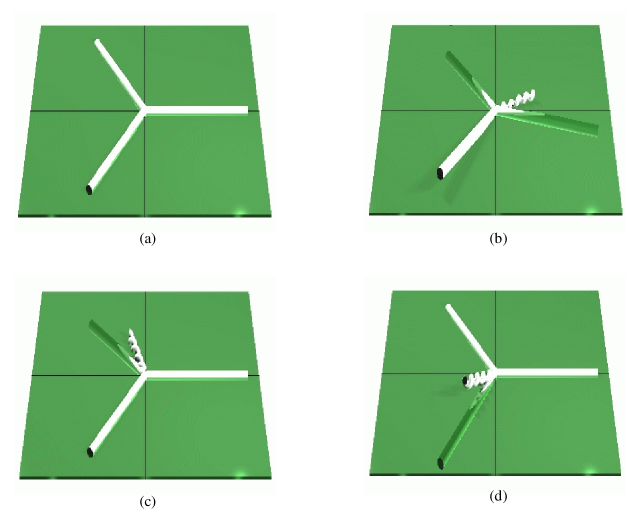
Figure 2: (a) Hard partons in a generic Born configuration. (b) Soft gluon $k$ (the short curly stick) is emitted in the right hemisphere. All three hard partons experience equal out-of-plane recoil, see (2.9). White (shadowed) partons have positive (negative) $x$-components of the momentum. (c) Soft gluon $k$ is emitted in the up-left region. According to (2.10), only parton #2 recoils (shadowed; has a negative $x$-components of the momentum). (d) The case of $k$ in the down-left region.

As we shall see in the next section, similar kinematical effects show up in the structure of the NP contribution as well.

(2.8) is an example of the rich information on the colour structure and on the geometry of the underlying event provided by this observable.

3 NP-effects in the distribution and mean

Similarly to other jet observables, the leading NP correction to the $K_{\mbox{\scriptsize out}}$ distribution originates from radiation of small transverse momentum gluons (“gluers”) by the $q\bar{q}g$ antenna. It is important that, at the NP level, the parton recoils $q_{a}$ not only contribute to the observable ((1.3), (1.4)), as in the PT case, but also affect the radiator itself. In the linear approximation in $1/Q$, the radiator acquires a NP correction in the form

$$R^{\mbox{\scriptsize NP}}\>=\>\nu\cdot\lambda^{\mbox{\scriptsize NP}}\,\sum_{a=1}^{3}C_{a}\,\ln\frac{Q^{\mbox{\scriptsize NP}}_{a}}{|q_{ax}|}.$$ (3.1)

Here the variable $\nu$ in (3.1) is Mellin conjugated to $K_{\mbox{\scriptsize out}}$, and $\lambda^{\mbox{\scriptsize NP}}$ (of dimension of mass) is a standard NP parameter which can be related to the momentum integral of the QCD coupling in the infrared region and parameterizes the $1/Q$ power correction. $Q^{NP}_{a}\sim Q$ are the relevant scales which have the same geometric structure as the PT scales (2.4), and differ from those by a finite numerical factor [5].

The logarithmic enhancement of the NP contribution (3.1) is similar to that for the jet Broadening observables (see [7]). It originates from the logarithmic integration over the gluer angle $\theta$ with respect to the direction of the emitting parton $p_{a}$, starting from large angles $\theta={\cal{O}}\left(1\right)$ down to the angle of the hard parton $\theta_{\min}\sim|q_{ax}|/Q$. Radiation at smaller angles corresponds to collinear splitting and does not contribute to the observable due to real-virtual cancellation.

It is clear from the structure of the integral involving the Mellin exponent $e^{\nu K_{\mbox{\scriptsize out}}}$ and the exponent of the sum of the PT and NP radiators that the correction term (3.1) being linear in $\nu$ results in a shift of the argument $K_{\mbox{\scriptsize out}}$ of the PT distribution. To find this shift one has to perform the $q_{ax}$ integrals, for a given $K_{\mbox{\scriptsize out}}$, taking into consideration the phase space constraints (1.4).

To explain the structure of the answer let us introduce the distributions ${\cal{D}}_{a}(|q_{ax}|)$ of the parton recoil momenta. For the leading jet #1 it is given by the derivative of the DL Sudakov exponent:

$${\cal{D}}_{1}(q)=\frac{d}{d\ln q}\>e^{-R_{1}(q^{-1})},\quad q=|q_{1x}|\,.$$ (3.2)

The average value of the logarithm in (3.1) (the logarithm of the inverse quark angle) evaluated under the restriction $|q_{1x}|<K_{\mbox{\scriptsize out}}$ becomes

$$\begin{split}\left\langle\ln\frac{Q_{1}^{\mbox{\scriptsize NP}}}{|q_{1x}|}\right\rangle_{|q_{1x}|<K_{\mbox{\scriptsize out}}}&\equiv e^{R_{1}(K_{\mbox{\scriptsize out}}^{-1})}\int_{0}^{K_{\mbox{\scriptsize out}}}\frac{dq}{q}\,\ln\frac{Q_{1}^{\mbox{\scriptsize NP}}}{q}{\cal{D}}_{1}(q)=\ln\frac{Q_{1}^{\mbox{\scriptsize NP}}}{K_{\mbox{\scriptsize out}}}+E_{1}(K_{\mbox{\scriptsize out}}^{-1})\>,\\ E_{1}(K_{\mbox{\scriptsize out}}^{-1})&\equiv\int_{0}^{K_{\mbox{\scriptsize out}}}\frac{dq}{q}\,e^{-R_{1}(q^{-1})+R_{1}(K_{\mbox{\scriptsize out}}^{-1})}.\end{split}$$ (3.3)

For the partons $\#2$ and $\#3$ in the $L$-hemisphere the situation is more delicate. As we already know from the plane constraints, in order to inhibit the recoil of a left-hemisphere parton $\#a$ we have to veto radiation both from $\#a$ and the right-hemisphere parton $\#1$. Therefore,

$${\cal{D}}_{a}(q)=\frac{d}{d\ln q}\>e^{-R_{a}(q^{-1})-R_{1}(q^{-1})},\qquad a=2,3\,,$$ (3.4)

and the average logarithms become

$$\begin{split}\left\langle\ln\frac{Q_{a}^{\mbox{\scriptsize NP}}}{|q_{ax}|}\right\rangle_{|q_{ax}|<K_{\mbox{\scriptsize out}}}&=\ln\frac{Q_{a}^{\mbox{\scriptsize NP}}}{K_{\mbox{\scriptsize out}}}+E_{a}(K_{\mbox{\scriptsize out}}^{-1})\\ E_{a}(K_{\mbox{\scriptsize out}}^{-1})&\equiv\int_{0}^{K_{\mbox{\scriptsize out}}}\frac{dq}{q}\,e^{-R_{a}(q^{-1})-R_{1}(q^{-1})+R_{a}(K_{\mbox{\scriptsize out}}^{-1})+R_{1}(K_{\mbox{\scriptsize out}}^{-1})}\>,\qquad a=2,3\,.\end{split}$$ (3.5)

In the limit of moderately small $K_{\mbox{\scriptsize out}}$, so that $\alpha_{\mbox{\scriptsize s}}\ln^{2}\frac{Q}{K_{\mbox{\scriptsize out}}}\ll 1$, these functions can be approximately evaluated to give

$$\begin{split}E_{1}(K_{\mbox{\scriptsize out}}^{-1})&=\frac{\pi}{2\sqrt{C_{1}\alpha_{\mbox{\scriptsize s}}(Q)}}-\ln\frac{Q}{K_{\mbox{\scriptsize out}}}\>+\>{\cal{O}}\left(1\right)\,,\\ E_{a}(K_{\mbox{\scriptsize out}}^{-1})&=\frac{\pi}{2\sqrt{(C_{a}+C_{1})\alpha_{\mbox{\scriptsize s}}(Q)}}-\ln\frac{Q}{K_{\mbox{\scriptsize out}}}\>+\>{\cal{O}}\left(1\right)\,,\quad a=2,3\,.\end{split}$$ (3.6)

Starting from large values $\propto 1/\sqrt{\alpha_{\mbox{\scriptsize s}}}$, the functions $E$ decrease with $K_{\mbox{\scriptsize out}}$. They vanish as $E\propto 1/r^{\prime}(K_{\mbox{\scriptsize out}}^{-1})$ in the limit of extremely small $K_{\mbox{\scriptsize out}}$, such that the Sudakov suppression becomes very strong, $r^{\prime}=\frac{2\alpha_{\mbox{\scriptsize s}}}{\pi}\ln\frac{Q}{K_{\mbox{\scriptsize out}}}\gg 1$. We conclude that the average logarithms of the parton recoil angles in (3.1) stay at large constant values ${\cal{O}}\left(1/\sqrt{\alpha_{\mbox{\scriptsize s}}}\right)$, given by the the first terms on r.h.s. of (3.6), in a broad region $1\mathrel{\mathchoice{\lower 3.6pt\vbox{\halign{$\mathsurround=0pt\displaystyle\hfil#\hfil$\cr>\crcr\sim\crcr}}}{\lower 3.6pt\vbox{\halign{$\mathsurround=0pt\textstyle\hfil#\hfil$\cr>\crcr\sim\crcr}}}{\lower 3.6pt\vbox{\halign{$\mathsurround=0pt\scriptstyle\hfil#\hfil$\cr>\crcr\sim\crcr}}}{\lower 3.6pt\vbox{\halign{$\mathsurround=0pt\scriptscriptstyle\hfil#\hfil$\cr>\crcr\sim\crcr}}}}K_{\mbox{\scriptsize out}}/Q\gg\exp(-1/\sqrt{\alpha_{\mbox{\scriptsize s}}})$, and follow $\ln\frac{Q}{K_{\mbox{\scriptsize out}}}$ for still smaller values of $K_{\mbox{\scriptsize out}}$. On the basis of these considerations we can obtain the results for the distribution and mean.

3.1 NP correction to $\left\langle K_{\mbox{\scriptsize out}}\right\rangle$

The NP correction to the mean value of $K_{\mbox{\scriptsize out}}$ is given by the $\nu$-derivative at $\nu=0$ of the NP radiator in (3.1). To evaluate $\left\langle K_{\mbox{\scriptsize out}}\right\rangle$ it suffices to take the unrestricted average of $\ln(Q/|q_{ax}|)$ by setting $K_{\mbox{\scriptsize out}}$ in (3.3), (3.5) at their maximum values, i.e. $E_{a}(1/Q_{a}^{\mbox{\scriptsize NP}})$. The accurate answer that includes first subleading corrections reads [5]

$$\left\langle K_{\mbox{\scriptsize out}}\right\rangle=\left\langle K_{\mbox{\scriptsize out}}\right\rangle^{\mbox{\scriptsize PT}}+\lambda^{\mbox{\scriptsize NP}}\cdot\left\langle K_{\mbox{\scriptsize out}}\right\rangle^{\mbox{\scriptsize NP}}\!\!\!,\quad\left\langle K_{\mbox{\scriptsize out}}\right\rangle^{\mbox{\scriptsize NP}}=\sum_{a=1}^{3}C_{a}\,E_{a}\left(\frac{1}{Q_{a}^{\mbox{\scriptsize NP}}}\right)\left(1+{\cal{O}}\left(\alpha_{\mbox{\scriptsize s}}\right)\right)\,.$$ (3.7)

Analytically,

$$\left\langle K_{\mbox{\scriptsize out}}\right\rangle^{\mbox{\scriptsize NP}}\simeq\frac{\pi}{2\sqrt{\alpha_{\mbox{\scriptsize s}}(Q)}}\left(\frac{C_{1}}{\sqrt{C_{1}}}+\frac{C_{2}}{\sqrt{C_{1}+C_{2}}}+\frac{C_{3}}{\sqrt{C_{1}+C_{3}}}\right)\>+\>{\cal{O}}\left(1\right).$$ (3.8)

Since combinations of charges appear in the denominators, we remark that the jets do not contribute independently to the mean at the NP level.

3.2 NP shift of the PT ${K_{\mbox{\scriptsize out}}}$-distribution

The NP shift of the distribution contains two structures, the additive and the non-additive pieces:

$$\Sigma(K_{\mbox{\scriptsize out}})=\Sigma^{\mbox{\scriptsize PT}}(K_{\mbox{\scriptsize out}}-\lambda^{\mbox{\scriptsize NP}}\delta K),\quad\delta K=\sum_{a=1}^{3}C_{a}\left(\Delta_{a}+\Delta^{\prime}_{a}\right).$$ (3.9)

The additive contribution is

$$\Delta_{a}(K_{\mbox{\scriptsize out}})=\ln\frac{Q_{a}^{\mbox{\scriptsize NP}}}{K_{\mbox{\scriptsize out}}}+\psi(1+R^{\prime})+\gamma_{E}\>\simeq\>\ln\frac{Q}{K_{\mbox{\scriptsize out}}}\,.$$ (3.10)

The other contribution has the following structure (a more accurate expression can be found in [5]):

$$\begin{split}\Delta_{1}^{\prime}(K_{\mbox{\scriptsize out}})&\simeq\frac{C_{2}+C_{3}}{C_{T}}\,E_{1}(K_{\mbox{\scriptsize out}}^{-1})\,,\\ \Delta_{2}^{\prime}(K_{\mbox{\scriptsize out}})&\simeq\frac{C_{3}}{C_{T}}\,E_{2}(K_{\mbox{\scriptsize out}}^{-1})\,,\\ \Delta_{3}^{\prime}(K_{\mbox{\scriptsize out}})&\simeq\frac{C_{2}}{C_{T}}\,E_{3}(K_{\mbox{\scriptsize out}}^{-1})\,.\end{split}$$ (3.11)

The additive contribution $\Delta$ has a simple origin. It corresponds to the situation where all three emitters have recoil momenta of order $K_{\mbox{\scriptsize out}}$. Therefore, this contribution to the shift follows immediately from the NP radiator (3.1) with $|q_{ax}|\sim K_{\mbox{\scriptsize out}}$. Such a situation is typical of well-developed parton systems with many secondary partons. In the kinematical region $\alpha_{\mbox{\scriptsize s}}\ln^{2}\frac{Q}{K_{\mbox{\scriptsize out}}}\gg 1$ the additive term $\Delta$ takes over $\Delta^{\prime}$, and fully dominates in the region $r^{\prime}=\frac{2\alpha_{\mbox{\scriptsize s}}}{\pi}\ln\frac{Q}{K_{\mbox{\scriptsize out}}}>1$:

$$\delta K=\left(\,C_{1}+C_{2}+C_{3}\,\right)\ln\frac{Q}{K_{\mbox{\scriptsize out}}}\>+\>{\cal{O}}\left(1\right)\,,\qquad\frac{\alpha_{\mbox{\scriptsize s}}}{\pi}\ln^{2}\frac{Q}{K_{\mbox{\scriptsize out}}}\gg 1\,.$$ (3.12)

On the contrary, for $\alpha_{\mbox{\scriptsize s}}\ln^{2}\frac{Q}{K_{\mbox{\scriptsize out}}}\ll 1$ there are few secondary partons, and the non-additive contribution $\Delta^{\prime}$ is dominant. To analyse this situation let us relate the NP correction to the integrated spectrum $\Sigma$ to the differential distribution and expand the latter to first order in $\alpha_{\mbox{\scriptsize s}}$ in the region $\alpha_{\mbox{\scriptsize s}}\ln^{2}\frac{Q}{K_{\mbox{\scriptsize out}}}\ll 1$:

$$\Sigma-\Sigma^{\mbox{\scriptsize PT}}\simeq-\lambda^{\mbox{\scriptsize NP}}\delta K\cdot\frac{d\Sigma^{\mbox{\scriptsize PT}}}{dK_{\mbox{\scriptsize out}}}\simeq-\lambda^{\mbox{\scriptsize NP}}\frac{R^{\prime}}{K_{\mbox{\scriptsize out}}}\cdot\delta K;\quad R^{\prime}=C_{T}r^{\prime}\,.$$ (3.13)

Putting together the $\Delta$ and $\Delta^{\prime}$ terms in $\delta K$ we can then represent the answer as

$$R^{\prime}\cdot\delta K\simeq R^{\prime}\cdot C_{T}\ln\frac{Q}{K_{\mbox{\scriptsize out}}}+R_{2}^{\prime}\cdot\left(C_{1}E_{1}+C_{3}E_{3}\right)+R_{3}^{\prime}\cdot\left(C_{1}E_{1}+C_{2}E_{2}\right),$$ (3.14)

where all the $E$-functions are evaluated at $K_{\mbox{\scriptsize out}}^{-1}$. In the region under consideration we can use the approximation (3.6),

$$E_{a}(K_{\mbox{\scriptsize out}}^{-1})=E_{a}(Q^{-1})-\ln\frac{Q}{K_{\mbox{\scriptsize out}}}\>=\>\left\langle K_{\mbox{\scriptsize out}}\right\rangle^{\mbox{\scriptsize NP}}_{a}-\ln\frac{Q}{K_{\mbox{\scriptsize out}}},$$ (3.15)

where $\left\langle K_{\mbox{\scriptsize out}}\right\rangle^{\mbox{\scriptsize NP}}_{a}$ is the NP contribution to the mean associated with parton $\#a$ in (3.7). Assembling the logarithmic pieces we arrive at

$$\begin{split}R^{\prime}\cdot\delta K&\simeq R_{1}^{\prime}\cdot C_{T}\,\ln\frac{Q}{K_{\mbox{\scriptsize out}}}\\ &+R_{2}^{\prime}\cdot\left(\left\langle K_{\mbox{\scriptsize out}}\right\rangle^{\mbox{\scriptsize NP}}_{1}+C_{2}\,\ln\frac{Q}{K_{\mbox{\scriptsize out}}}+\left\langle K_{\mbox{\scriptsize out}}\right\rangle^{\mbox{\scriptsize NP}}_{3}\right)\\ &+R_{3}^{\prime}\cdot\left(\left\langle K_{\mbox{\scriptsize out}}\right\rangle^{\mbox{\scriptsize NP}}_{1}+\left\langle K_{\mbox{\scriptsize out}}\right\rangle^{\mbox{\scriptsize NP}}_{2}+C_{3}\,\ln\frac{Q}{K_{\mbox{\scriptsize out}}}\right).\end{split}$$ (3.16)

Now we are ready to discuss the meaning of this expression.

Making notice that the factor $R_{a}^{\prime}$ corresponds to the radiation of a perturbative gluon off the hard parton $\#a$, we see that the first line describes PT emission in the $R$ hemisphere. In this case all three hard partons experience equal recoil, $|q_{ax}|=K_{\mbox{\scriptsize out}}/4$ (see Fig. 2b), and the logarithmic factors in the NP radiator (3.1) are the same for all three gluers.

The second and third lines correspond to PT gluon emission off the parton #2 and #3. In the former case $|q_{2x}|=K_{\mbox{\scriptsize out}}/2$, while the other two partons remain in the plane ($q_{1x}=q_{3x}=0$) (see Fig. 2c). Now, NP gluer radiation off #2 brings in a logarithmic correction as above. At the same time, the logarithms $\ln Q/|q_{ax}|$, $a=1,3$ are integrated with the corresponding Sudakov distributions ${\cal{D}}_{a}$ producing the contributions identical to those to the mean.

Substituting $\left\langle K_{\mbox{\scriptsize out}}\right\rangle^{\mbox{\scriptsize NP}}_{a}$ from (3.8), an approximate expression for the NP shift becomes

$$\begin{split}\delta K&=\left[\,\frac{(C_{2}+C_{3})\sqrt{C_{1}}}{C_{T}}+\frac{C_{2}C_{3}}{C_{T}}\left(\frac{1}{\sqrt{C_{1}+C_{2}}}+\frac{1}{\sqrt{C_{1}+C_{3}}}\right)\right]\frac{\pi}{2\sqrt{\alpha_{\mbox{\scriptsize s}}(Q)}}\\ &+\left[\,C_{1}+\frac{C_{2}^{2}+C_{3}^{2}}{C_{T}}\,\right]\ln\frac{Q}{K_{\mbox{\scriptsize out}}}\>+\>{\cal{O}}\left(1\right)\,,\qquad\frac{\alpha_{\mbox{\scriptsize s}}}{\pi}\ln^{2}\frac{Q}{K_{\mbox{\scriptsize out}}}\ll 1\,.\end{split}$$ (3.17)

The general expression for the NP shift (3.9)–(3.11) interpolates between the two limiting regimes (3.17) and (3.12).

4 Conclusions

We have presented the results and discussed the main physical ingredients of the QCD analysis of the out-of-event-plane momentum distribution in 3-jet events. It aims at improving the accuracy of the theoretical description of the final state structure of hard processes involving more than two jets. It should be possible to generalize the present approach to analyse production of two large-$p_{\perp}$ jets in DIS and production of a jet recoiling against $W^{\pm}$, $Z^{0}$ or a large-$p_{\perp}$ photon in hadron-hadron collisions.

The most interesting feature of the $K_{\mbox{\scriptsize out}}$ distribution is the non-additivity of contributions due to the radiation off the three jets. In the PT contribution it occurs at the level of a subleading SL correction, while in the $1/Q$ NP correction terms it shows up at the leading level via peculiar combinations of colour charges like $(C_{F}+C_{A})^{-\mbox{\small$\frac{1}{2}$}}$ (see (3.8), (3.17)). These can be traced back to the specific pattern of parton recoil due to the geometry of the event plane.

Technical details of the calculations and the final expressions within SL accuracy can be found in [4, 5]. The relative ${\cal{O}}\left(\alpha_{\mbox{\scriptsize s}}\right)$ correction in (1.5) has been computed [8] by matching the expansion of the approximate resummed PT formula from [4] with the ${\cal{O}}\left(\alpha_{\mbox{\scriptsize s}}^{2}\right)$ calculation of the differential $K_{\mbox{\scriptsize out}}$ distribution provided by four-parton event generators. (It is possible, in principle, to further improve the result by including the ${\cal{O}}\left(\alpha_{\mbox{\scriptsize s}}^{2}\right)$ term in the non-logarithmic correction factor with the help of five-parton generators.)

Predictions for the $K_{\mbox{\scriptsize out}}$ distribution and means in $q\bar{q}\gamma$ events can be obtained from the above formulae by simply setting to zero the colour charge corresponding to the gluon ($C_{3}=0$ in the colour configuration of Fig. 1.)

Along the same lines the PT and NP predictions can be derived for the mean and the distribution of $K_{\mbox{\scriptsize out}}$ in the $R$-hemisphere, rather than $K_{\mbox{\scriptsize out}}$ of the event as a whole. The corresponding perturbative formulae are much simpler, and so are the NP expressions. They can be essentially obtained by setting $C_{2}=C_{3}=0$ in the above expressions for the total $K_{\mbox{\scriptsize out}}$. (There is an additional difficulty, though, in calculating the proper scales $Q^{\mbox{\scriptsize PT}}$ and $Q^{\mbox{\scriptsize NP}}$ with subleading accuracy, due to kinematical complications.)

Acknowledgements

We are grateful to Gavin Salam for discussions and suggestions.

References

• [1] S. Catani, L. Trentadue, G. Turnock and B.R. Webber, Nucl. Phys. B407 (1993) 3;
S. Catani and B.R. Webber, Phys. Lett. B427 (1998) 377 [hep-ph/9801350];
S. Catani, G. Turnock and B.R. Webber, Phys. Lett. B295 (1992) 269;
Yu.L. Dokshitzer, A. Lucenti, G. Marchesini and G.P. Salam, JHEP 01 (1998) 011 [hep-ph/9801324];
V. Antonelli, M. Dasgupta and G.P. Salam, JHEP 02 (2000) 001 [hep-ph/9912488].
• [2] G.P. Korchemsky and G. Sterman, Nucl. Phys. B437 (1995) 415 [hep-ph/9411211];
B.R. Webber, Phys. Lett. B339 (1994) 148 [hep-ph/9408222]; see also Proc. Summer School on Hadronic Aspects of Collider Physics, Zuoz, Switzerland, August 1994, ed. M.P. Locher (PSI, Villigen, 1994) [hep-ph/9411384];
Yu.L. Dokshitzer and B.R. Webber, Phys. Lett. B352 (1995) 451 [hep-ph/9504219];
R. Akhoury and V.I. Zakharov, Phys. Lett. B357 (1995) 646 [hep-ph/9504248]; Nucl. Phys. B465 (1996) 295 [hep-ph/9507253];
Yu.L. Dokshitzer, V.A. Khoze and S.I. Troyan, Phys. Rev. D53 (1996) 89 [hep-ph/9506425];
Yu.L. Dokshitzer, G. Marchesini and B.R. Webber, Nucl. Phys. B469 (1996) 93 [hep-ph/9512336];
P. Nason and M.H. Seymour, Nucl. Phys. B454 (1995) 291 [hep-ph/9612353];
Yu.L. Dokshitzer, A. Lucenti, G. Marchesini and G.P. Salam, Nucl. Phys. B511 (1998) 396 [hep-ph/9707532] G.P. Korchemsky, G. Oderda and G. Sterman, in Deep Inelastic Scattering and QCD, 5${}^{\mbox{\scriptsize th}}$ International Workshop, Chicago, IL, April 1997, p. 988 [hep-ph/9708346];
M. Beneke, Phys. Rep. 317 (1999) 1.
• [3] R. Orava, V. Nomokonov, R. Vuopionpera, K. Vaisanen, V. A. Khoze and K. Lassila, Eur. Phys. J. C5 (1998) 471.
• [4] A. Banfi, Yu.L. Dokshitzer, G. Marchesini and G. Zanderighi, JHEP 07 (2000) 002 [hep-ph/0004027]
• [5] A. Banfi, Yu.L. Dokshitzer, G. Marchesini and G. Zanderighi, under preparation.
• [6] S. Catani, G. Marchesini and B.R. Webber, Nucl. Phys. B349 (1991) 635.
• [7] Yu.L. Dokshitzer, A. Lucenti, G. Marchesini and G.P. Salam, JHEP 05 (1998) 003 [hep-ph/9802381],
Yu.L. Dokshitzer, G. Marchesini and G.P. Salam, Eur. Phys. J. C3 (1999) 1 [hep-ph/9812487].
• [8] A. Banfi, G. Salam, G. Zanderighi, under preparation.