LU TP 00-44

hep-ph/0010265

October 2000

WEAK INTERACTIONS OF LIGHT FLAVOURS
Johan Bijnens
Dept. of Theoretical Physics, Lund University,

Sölvegatan 14A, S22362 Lund, Sweden

An overview is given of weak interaction physics of the light flavours. It starts with the definition of the CKM matrix and the measurement of its components in the light-flavour sector via semi-leptonic decays. The main part of the lectures is devoted to non-leptonic decays with a main emphasis on analytical calculations of $K\to\pi\pi$ and $K\leftrightarrow\overline{K^{0}}$. It finishes with an overview of Chiral Perturbation Theory in $K\to 3\pi$ and of rare Kaon decays.

1 Introduction

These lectures on the weak interaction are not out of place at a school devoted to the strong interaction. As will be extremely obvious in the remainder the main problem in dealing with the weak interactions of quarks is that they are confined in hadrons and thus the non-perturbative regime of the strong interactions becomes very important.

The lectures first present an introduction as to why we want to study this type of physics and the Cabibbo-Kobayashi-Maskawa matrix. The second part then discusses semi-leptonic decays. The relevant physics here is the determination of $|V_{ud}|$ and $|V_{us}|$. This will allow us to test precisely the unitarity relation

$$|V_{ud}|^{2}+|V_{us}|^{2}+|V_{ub}|^{2}=1\,.$$ (1)

The main part of the lectures is dedicated to the calculation of non-leptonic decays and in particular of $K\to\pi\pi$ and $K$-$\overline{K^{0}}$ mixing. This tests the $CP$-violating part of the standard model and in particular the consistency of the whole $CKM$-ansatz in the Higgs-Fermion part of the standard model. Here Kaon physics is very complementary to $B$-physics. Loop diagrams and QCD effects are very important.

We conclude by a short overview of applications of Chiral Perturbation Theory (CHPT) to $K\to 3\pi$ and of rare Kaon decays, those which are first tests of QCD and the Chiral Lagrangian and those important for the SM (and beyond) weak interaction part.

The lectures by Ben Grinstein [1] cover the complementary aspects in $B$-physics. Gerhard Ecker [2] described Chiral Perturbation Theory (CHPT). Those techniques also play an important role here. Finally, Chris Sachrajda [3] described the present status of the lattice QCD calculations of basically the same quantities.

Some other lecture notes or review articles covering similar topics are Refs. [4] to [8].

2 Standard Model

The Standard Model Lagrangian has four parts:

$${\cal L}_{SM}=\displaystyle\underbrace{{\cal L}_{H}(\phi)}_{\mbox{Higgs}}+\underbrace{{\cal L}_{G}(W,Z,G)}_{\mbox{Gauge}}\displaystyle+\underbrace{\sum_{\psi=\mbox{fermions}}\bar{\psi}iD\hskip-6.99997pt/\hskip 3.99994pt\psi}_{\mbox{gauge-fermion}}+\underbrace{\sum_{\psi,\psi^{\prime}=\mbox{fermions}}g_{\psi\psi^{\prime}}\bar{\psi}\phi\psi^{\prime}}_{\mbox{Yukawa}}$$

The experimental tests on the various parts are at a very different level:
gauge-fermion Very well tested at LEP-1 and other precision measurements Higgs Hardly tested, real tests coming up now at LEP-2, Tevatron and LHC in the future Gauge part Well tested in QCD, partly in electroweak at LEP-2 Yukawa The real testing ground for weak interactions and the main source of the number of standard model parameters.

There are three discrete symmetries that play a special role, they are
$\bullet$ C Charge Conjugation
$\bullet$ P Parity
$\bullet$ T Time Reversal
QCD and QED conserve C,P,T separately. Local Field theory by itself implies CPT. The fermion and Higgs part of the SM-lagrangian conserves CP and T as well.

The only part that violates CP and as a consequence also T is the Yukawa part. The Higgs part is responsible for two parameters, the gauge part for three and the Higgs-Fermion part contains in principle 27 complex parameters, neglecting Yukawa couplings to neutrinos. Luckily most of the 54 real parameters in the Yukawa sector are unobservable. After diagonalizing the lepton sector there only the three charged lepton masses remain. The quark sector can be similarly diagonalized leading to 6 quark masses, but some parts remain in the difference between weak interaction eigenstates and mass-eigenstates. The latter is conventionally put in the couplings of the charged $W$-boson, which is given by

$$\displaystyle-\frac{g}{2\sqrt{2}}W^{-}_{\mu}\left(\overline{u}^{\alpha}~{}\overline{c}^{\alpha}~{}\overline{t}^{\alpha}\right)\gamma^{\mu}\left(1-\gamma_{5}\right)\left(\begin{array}[]{ccc}V_{ud}&V_{us}&V_{ub}\\ V_{cd}&V_{cs}&V_{cb}\\ V_{td}&V_{ts}&V_{td}\end{array}\right)\left(\begin{array}[]{c}d_{\alpha}\\ s_{\alpha}\\ b_{\alpha}\end{array}\right)$$ (8)

$$\displaystyle-\frac{g}{2\sqrt{2}}W^{-}_{\mu}\sum_{\ell=e,\mu,\tau}\bar{\nu}_{\ell}\gamma^{\mu}\left(1-\gamma_{5}\right)\ell$$

C and P are broken by the $(1-\gamma_{5})$ in the couplings. CP is broken if $V_{CKM}=\left(V_{ij}\right)$ is (irreducibly) complex.

Figure 1: Muon decay: the main source of our knowledge of $g$.

The couplings constant $g$ together with the mass $M_{W}^{2}$ can be determined from the Fermi constant as measured in muon decay. The relevant corrections are known to two-loop level. The most recent calculations and earlier references can be found in [9]. The result is

$$G_{F}=\frac{g^{2}}{8M_{W}^{2}}=1.16639(1)\cdot 10^{-5}~{}\mbox{GeV}^{-2}\,.$$ (9)

The Cabibbo-Kobayashi-Maskawa matrix $V_{CKM}=\left(V_{ij}\right)$ results from diagonalizing the quark mass terms resulting from the Yukawa terms and the Higgs vacuum expectation value. It is a general unitary matrix but the phases of the quark fields can be redefined. This allows to remove 5 of the 6 phases present in a general unitary 3 by 3 matrix. The matrix $V_{CKM}$ thus contains three phases and one mixing angle. The Particle Data Group preferred parametrization is [10]

$$\left(\begin{array}[]{ccc}c_{12}c_{13}&s_{12}c_{13}&s_{13}e^{-i\delta_{13}}\\ -s_{12}c_{23}-c_{12}s_{23}s_{13}e^{i\delta_{13}}&c_{12}c_{23}-s_{12}s_{23}s_{13}e^{i\delta_{13}}&s_{23}c_{13}\\ s_{12}s_{23}-c_{12}c_{23}s_{13}e^{i\delta_{13}}&-c_{12}s_{23}-s_{12}c_{23}s_{13}e^{i\delta_{13}}&c_{23}c_{13}\,.\end{array}\right)$$ (10)

Using the measured experimental values, see below and [1],

$$s_{12}=\sin\theta_{12}\approx 0.2;s_{23}\approx 0.04\mbox{ and }s_{13}\approx 0.003$$ (11)

an approximate parametrization, known as the Wolfenstein parametrization, can be given. This is defined via $s_{12}c_{13}\equiv\lambda$; $s_{23}c_{13}\equiv A\lambda^{2}$ and $s_{13}e^{-i\delta_{13}}\equiv A\lambda^{3}(\rho-i\eta)$. To order $\lambda^{4}$ the CKM-matrix is

$$\left(\begin{array}[]{ccc}1-\frac{\lambda^{2}}{2}&\lambda&A\lambda^{3}(\rho-i\eta)\\ -\lambda&1-\frac{\lambda^{2}}{2}&A\lambda^{2}\\ A\lambda^{3}(1-\rho-i\eta)&-A\lambda^{2}&1\end{array}\right)$$ (12)

3 Semi-leptonic Decays

3.1 $V_{ud}$

The underlying idea always the same. The vector current has matrix-element one at zero momentum transfer because of the underlying vector Ward identities. The element $V_{ud}$ is measured in three main sets of decays.

• neutron: Here we use in addition that the axial current effect is actually measurable via the angular distribution of the electron. So $\Gamma(n\to pe^{-}\bar{\nu})\sim G_{n}^{2}(1+3g_{A}^{2}/g_{V}^{2})A$
  with $A$ calculable but containing photon loops. Using the value for $g_{A}/g_{V}$ and the neutron lifetime of the 98 particle data book[11] and the calculations of radiative corrections quoted in [12] I obtain

  $$|V_{ud}|=0.9792(40)\,.$$ (13)

  At present the errors are dominated by the measurement of $g_{A}/g_{V}$. This could change in the near future.

• Nuclear superallowed $\beta$-decays: $0^{+}\to 0^{+}$ The main advantages here are that only the vector current can contribute and that very accurate experimental results are available. The disadvantage is that the charge symmetry breaking, or isospin, effects and the photonic radiative corrections are nuclear structure dependent with an unknown error. The quoted theory errors are such that the measurements for different nuclei are in contradiction with each other. In [11] they therefore quote

  $$|V_{ud}|=0.9740(10)\,.$$ (14)

• Pion $\beta$-decay: $\pi^{+}\to\pi^{0}e^{+}\bar{\nu}$ The theory here is very clean and improvable using CHPT. The disadvantage is that the branching ratio is about $10^{-8}$, known to about 4%. Experiments at PSI are in progress to get 0.5%.

In the future better experimental precision in neutron and $\pi$ $\beta$-decay should improve the determination. $|V_{ud}|$ is by far the best directly determined CKM-matrix element.

3.2 $V_{us}$

Again we use the fact that the matrix-element of a conserved vector current is one at zero momentum. But compared to the previous subsection we have additional complications:
$\bullet$ The vector current is $\bar{s}\gamma_{\mu}u$ so corrections are $(m_{s}-m_{u})^{2}$ and not $(m_{d}-m_{u})^{2}$ so they are naively larger.
$\bullet$ A longer extrapolation to the zero-momentum point is needed.
The relevant semi-leptonic decays can be measured in hyperon or in Kaon decays.

Hyperon $\beta$-decays (e.g. $\Sigma^{-}\to ne^{-}\bar{\nu},\Lambda\to pe^{-}\bar{\nu}$): Here there are large theoretical problems. In CHPT the corrections are large and many new parameters show up. In addition the series does not converge too well. Curiously enough, using lowest order CHPT with model-corrections works OK. For references consult the relevant section of [10, 11]. This area needs theoretical work very badly.

Kaon $\beta$-decays (e.g. $K^{+}\to\pi^{0}e^{+}\nu$): Both theory and data are old by now. The theory was done by Leutwyler and Roos [13]. The analysis uses old-fashioned photonic loops for the electro-magnetic corrections and one-loop CHPT for the strong corrections due to quark masses. Both aspects are at present being improved [14]. The latest data are from 1987 and the most precise ones are older. There is at present a proposal at BNL while KLOE at DAPHNE should also be able to improve the precision.

The result obtained from the last process is

$$|V_{us}|=0.2196\pm 0.0023\,.$$ (15)

We can now use this to test the unitarity relation

$$|V_{us}|^{2}+|V_{ud}|^{2}=0.9969\pm 0.0022$$ (16)

$|V_{ub}|^{2}$ is so small it is not visible in the precision shown here. This is a small discrepancy which should be understood but no real cause for worry at present.

3.3 Testing CHPT/QCD and determining CHPT parameters

In the sector of semi-leptonic Kaon decays CHPT unfolds all of its power. An extensive review can be found in [15] with a more recent update in [16]. There are of course also numerous model calculations and other approaches existing. An example of model calculations using Schwinger-Dyson equations is in [17]. Notice that the Schwinger-Dyson equations themselves do not constitute the model aspect but the assumptions made in their solutions.

I now simply list the main decays and which quantity they test and/or measure.

• $K\to\mu\nu$ ($K_{\ell 2}$) : Measurement of $F_{K}$. This known to two loops[18] in CHPT and the electromagnetic corrections have also been updated [19]

• $K\to\pi\ell\nu$ ($K_{\ell 3}$): $V_{us}$ and form-factors, see [15] and references therein.

• $K\to\pi\pi\ell\nu$ ($K_{\ell 4}$): Form-factors and a main source of CHPT input parameters. Known at two-loops in CHPT [20].

• $K\to\pi\ell\nu\gamma$ ($K_{\ell 3\gamma}$): Lots of form-factors with large corrections combining to a final small correction[21].

• $K(\pi)\to\ell\nu\gamma$ ($K(\pi)_{\ell 2\gamma}$): This has two form-factors, one normal and one anomalous. The interference between them allows to see the sign of the anomaly. This can also be done in $K_{\ell 4}$ and both confirm nicely the expectations[21, 15, 22].

4 Non-leptonic Decays: $K\to\pi\pi$ and $K$-$\overline{K^{0}}$ mixing

We have been rather successful in understanding the theory behind the semi-leptonic decays discussed in the previous section. Basically we always used CHPT or similar arguments to get at the coupling of the $W$-boson to hadrons. A similar simple approach fails completely for non-leptonic decays. I’ll first discuss the main qualitative problem that shows up in trying to estimate these decays, then the phenomenology involved in mixing phenomena and then proceed in the various steps needed to actually calculate these processes in the standard model. Finally some numerical results are presented.

4.1 The $\Delta I=1/2$ rule

The underlying problem appears when we try to calculate $K\to\pi\pi$ decays in a similar fashion as for the semi-leptonic decays. For $K^{+}\to\pi^{+}\pi^{0}$ we can draw two Feynman diagrams with a simple $W^{+}$ exchange as shown in Fig. 2.

p                           

Figure 2: The two naive $W^{+}$-exchange diagrams for $K^{+}\longrightarrow\pi^{+}\pi^{0}$.

The relevant $W^{+}$-hadron couplings have all been measured in semi-leptonic decays and so we have a unique prediction. Comparing this with the measured decay we get within a factor of two or so.

A much worse result appears when we try the same method for the neutral decay $K^{0}\to\pi^{0}\pi^{0}$. As shown in Fig. 3 there is no possibility to draw diagrams similar to those in Fig. 2. The needed vertices always violate charge-conservation.

Figure 3: No simple $W^{+}$-exchange diagram is possible for $K^{0}\longrightarrow\pi^{0}\pi^{0}$.

So we expect that the neutral decay should be small compared with the ones with charged pions. Well, if we look at the experimental results we see

$$\Gamma(K^{0}\longrightarrow\pi^{0}\pi^{0})= \displaystyle\frac{1}{2}\Gamma(K_{S}\longrightarrow\pi^{0}\pi^{0}) =2.3\;10^{-12}\mbox{ MeV}$$

$$\Gamma(K^{+}\longrightarrow\pi^{+}\pi^{0})= \displaystyle=1.1\;10^{-14}\mbox{ MeV}$$ (17)

So the expected zero one is by far the largest !!!

The same conundrum can be expressed in terms of the isospin amplitudes:

$$A[K^{0}\to\pi^{0}\pi^{0}]\equiv\sqrt{\frac{1}{3}}{A_{0}}-\sqrt{\frac{2}{3}}\,{A_{2}}$$

$$A[K^{0}\to\pi^{+}\pi^{-}]\equiv\sqrt{\frac{1}{3}}{A_{0}}+\frac{1}{\sqrt{6}}\,{A_{2}} A[K^{+}\to\pi^{+}\pi^{0}]\equiv\frac{\sqrt{3}}{2}{A_{2}}\,.$$ (18)

The above quoted experimental results can now be rewritten as

$$\left|\frac{A_{0}}{A_{2}}\right|=22.1$$ (19)

while the naive $W^{+}$-exchange discussed would give $\left|{A_{0}}/{A_{2}}\right|=\sqrt{2}\,.$ This discrepancy is known as the problem of the $\Delta I=1/2$ rule. The amplitude which changes the isospin $1/2$ to zero is much larger than the one that changes the isospin to 2 by $3/2$.

Some enhancement is easy to understand from final state $\pi\pi$-rescattering. Removing these and higher order effects in the light quark masses one obtains[23]

$$\left|\frac{A_{0}}{A_{2}}\right|=16.4\,.$$ (20)

Later we also need the amplitudes with the final state interaction phase removed via

$$A_{I}=-ia_{I}e^{i\delta_{I}}$$ (21)

for $I=0,2$. $\delta_{I}$ is the angular momentum zero isospin I scattering phase at the Kaon mass.

4.2 Phenomenology of $K$-$\overline{K^{0}}$ mixing

The $K^{0}$ and $\overline{K^{0}}$ states are the ones with $\bar{s}d$ and $\bar{d}s$ quark content respectively. Up to free phases in these states we can define the action of $CP$ on these states as

$$CP|K^{0}\rangle=-|\overline{K^{0}}\rangle\,.$$ (22)

We can construct eigenstates with a definite $CP$ transformation:

$$K^{0}_{1(2)}=\frac{1}{\sqrt{2}}\left(K^{0}-(+)\overline{K^{0}}\right)\quad\quad CP|K_{1(2)}=+(-)|K_{1(2)}\,.$$ (23)

Now the main decay mode of $K^{0}$-like states is $\pi\pi$. A two pion state with charge zero in spin zero is always CP even. Therefore the decay $K_{1}\to\pi\pi$ is possible but $K_{2}\to\pi\pi$ is impossible; $K_{2}\to\pi\pi\pi$ is possible. Phase-space for the $\pi\pi$ decay is much larger than for the three-pion final state. Therefore if we start out with a pure $K^{0}$ or $\overline{K^{0}}$ state its $\Rightarrow$ $K_{2}$ lives much longer than $K_{1}$. So after a, by microscopic standards, long time only the $K_{2}$ component survives.

In the early sixties, it pays off to do precise experiments, one actually measured [24]

$$\frac{\Gamma(K_{L}\to\pi^{+}\pi^{-})}{\Gamma(K_{L}\to\mbox{all})}=(2\pm 0.4)\cdot 10^{-3}\,.$$ (24)

So we see that CP is violated .

This leaves us with the questions:

• Does $K_{1}$ turn in to $K_{2}$ (mixing or indirect CP violation) ?

• Does $K_{2}$ decay directly into $\pi\pi$ (direct CP violation) ?

In fact, the answer to both is YES and is major qualitative test of the standard model Higgs-fermion sector.

Let us now describe the $K^{0}\overline{K^{0}}$ system in somewhat more detail. The Hamiltonian, seen as a two state system, is given by

$$i\frac{d}{dt}\left(\begin{array}[]{c}K^{0}\\ \overline{K}^{0}\end{array}\right)=\left(\begin{array}[]{cc}M_{11}-\frac{i}{2}\Gamma_{11}&M_{12}-\frac{i}{2}\Gamma_{12}\\ M_{21}-\frac{i}{2}\Gamma_{21}&M_{22}-\frac{i}{2}\Gamma_{22}\end{array}\right)\left(\begin{array}[]{c}K^{0}\\ \overline{K}^{0}\end{array}\right)$$ (25)

where $M=\left(M_{ij}\right)$ and $\Gamma=\left(\Gamma_{ij}\right)$ are hermitian two by two matrices. The Hamiltonian itself is allowed to have a non-hermitian part since we do not conserve probability here. The Kaons themselves can decay and the anti-hermitian part $\Gamma$ describes the decays of the Kaons to the “rest of the universe.”

CPT implies [5]

$$M_{11}=M_{22}\quad\Gamma_{11}=\Gamma_{22}\quad M_{12}=M_{21}^{*}\quad\Gamma_{12}=\Gamma_{21}^{*}$$ (26)

and this assumption can in fact be relaxed for tests of CPT.

Diagonalizing the Hamiltonian we obtain

$$K_{S(L)}=\frac{1}{\sqrt{1+|\tilde{\varepsilon}|^{2}}}\left(K_{1(2)}+\tilde{\varepsilon}K_{2(1)}\right)$$ (27)

as physical propagating states. Notice that they are not orthogonal.

For observables we now define:

$$\varepsilon=\frac{A(K_{L}\to(\pi\pi)_{I=0})}{A(K_{S}\to(\pi\pi)_{I=0})}\,,\quad\eta_{+-}=\frac{A(K_{L}\to\pi^{+}\pi^{-})}{A(K_{S}\to\pi^{+}\pi^{-})}\,,\quad\,,\quad\eta_{00}=\frac{A(K_{L}\to\pi^{0}\pi^{0})}{A(K_{S}\to\pi^{0}\pi^{0})}$$ (28)

and

$$\varepsilon^{\prime}=\frac{1}{\sqrt{2}}\left(\frac{A(K_{L}\to(\pi\pi)_{I=2})}{A(K_{S}\to(\pi\pi)_{I=0})}-\varepsilon\frac{A(K_{S}\to(\pi\pi)_{I=2})}{A(K_{S}\to(\pi\pi)_{I=0})}\right)\,.$$ (29)

The latter has been specifically constructed to remove the $K^{0}$-$\overline{K^{0}}$ transition. $|\varepsilon|$, $|\eta_{+-}|$ and $|\eta_{00}|$ are directly measurable.

We can now make a series of approximations that are experimentally valid,

$$|\mbox{Re}a_{0}|>>|\mbox{Re}a_{2}|>>|\mbox{Im}a_{0}|,|\mbox{Im}a_{2}|\quad\quad\quad|\varepsilon|,|\tilde{\varepsilon}|<<1\quad|\varepsilon^{\prime}|<<|\varepsilon|\,,$$ (30)

to obtain the usually quoted expressions

$$\varepsilon^{\prime}=\frac{i}{\sqrt{2}}e^{i(\delta_{2}-\delta_{0})}\frac{\mbox{Re}a_{2}}{\mbox{Re}a_{0}}\left(\frac{\mbox{Im}a_{2}}{\mbox{Re}a_{2}}-\frac{\mbox{Im}a_{0}}{\mbox{Re}a_{0}}\right)\quad\mbox{and}\quad\varepsilon=\tilde{\varepsilon}+i\frac{\mbox{Im}a_{0}}{\mbox{Re}a_{0}}\,.$$ (31)

For the latter we use $\Delta m=m_{L}-m_{S}\approx\frac{\Delta\Gamma}{2}$ and $\Gamma_{L}<<\Gamma_{S}$ and the fact that $\Gamma_{12}$ is dominated by $\pi\pi$ states and get

$$\varepsilon=\frac{1}{\sqrt{2}}e^{i\pi/4}\left(\frac{\mbox{Im}M_{12}}{\Delta m}+\frac{\mbox{Im}a_{0}}{\mbox{Re}a_{0}}\right)\,.$$ (32)

Putting all the above together we finally get to

$$\eta_{+-}=\varepsilon+\varepsilon^{\prime}\quad\mbox{and}\quad\eta_{00}=\varepsilon-2\varepsilon^{\prime}$$

Where you can see that $\varepsilon$ describes the indirect part and $\varepsilon^{\prime}$ the direct part, since the mixing contribution would be the same for $\eta_{+-}$ and $\eta_{00}$.

4.3 Experimental results and SM-diagrams

NA31	$(23.0\pm 6.5)\times 10^{-4}$
E731	$(7.4\pm 5.9)\times 10^{-4}$
KTeV	$(28.0\pm 4.1)\times 10^{-4}$
NA48 97	$(18.5\pm 7.3)\times 10^{-4}$
NA48 98	$(12.2\pm 4.9)\times 10^{-4}$
ALL	$(19.3\pm 2.4)\times 10^{-4}$

Table 1: Recent results on $\varepsilon^{\prime}/\varepsilon$. The total $\chi^{2}$ of the fit is $\chi^{2}/dof=11.1/5$.

Recent experimental results are

$$|\varepsilon|=2.28\cdot 10^{-3}\quad\mbox{and for}\quad\mbox{Re}\left(\frac{\varepsilon^{\prime}}{\varepsilon}\right)=\frac{1}{6}\left\{1-\left|\frac{\eta_{00}}{\eta_{+-}}\right|^{2}\right\}$$ (33)

we show the recent results in Table 1. The data are taken from [25].

In the standard model $K^{0}$$\overline{K^{0}}$ mixing comes from the box-diagram of Fig. 4(a)

Figure 4: (a) The box diagram contribution to $K^{0}$$\overline{K^{0}}$ mixing. Extra gluons etc. are not shown. (b) The Penguin.diagram contribution to $K\to\pi\pi$.

Since it contains $W$-couplings to all generations CP-violation from the CKM matrix is possible in this contribution. The Penguin diagram shown in Fig. 4(b) contributes to the direct CP-violation as given by $\varepsilon^{\prime}$. Again, $W$-couplings to all three generations show up so CP-violation is possible in $K\to\pi\pi$. This is a qualitative prediction of the standard model and borne out by experiment.

4.4 The steps from quarks to mesons in the weak interaction

The full calculation can be described by three steps depicted in Fig. 5.

ENERGY SCALE	FIELDS	Effective Theory
$M_{W}$	$W,Z,\gamma,g$; $\tau,\mu,e,\nu_{\ell}$; $t,b,c,s,u,d$	Standard Model
	$\Downarrow$ using OPE
$\lesssim m_{c}$	$\gamma,g$; $\mu,e,\nu_{\ell}$; $s,d,u$	QCD,QED,${\cal H}_{\mbox{eff}}^{|\Delta S|=1,2}$
	$\Downarrow$ ???
$M_{K}$	$\gamma$; $\mu,e,\nu_{\ell}$; $\pi$, $K$, $\eta$	CHPT

Figure 5: A schematic exposition of the various steps in the calculation of nonleptonic matrix-elements.

We cannot simply use one-loop perturbation theory for the short-distance part since $\log{\frac{M_{W}^{2}}{M_{K}^{2}}}$ and $\log{\frac{M_{t}^{2}}{M_{K}^{2}}}$ are large and their effects need to be resummed. This can be done using OPE and renormalization group methods.

First we integrated out the heaviest particles step by step using Operator Product Expansion methods. The steps OPE we descibe in the next subsections while step ??? we will split up in more subparts later.

4.5 Step I: from SM to OPE

The contribution from the standard model diagrams in Fig. 7

Figure 6: The standard model diagrams to be calculated at a high scale.

Figure 7: The diagrams needed for the matrix-elements calculated at a scale $\mu_{H}\approx m_{W}$ using the effective Hamiltonian.

we now replace with a contribution of an effective Hamiltonian given by

$${\cal H}_{\mbox{eff}}=\sum_{i}C_{i}(\mu)Q_{i}(\mu)\displaystyle{\cal H}_{\mbox{eff}}=\frac{G_{F}}{\sqrt{2}}V_{ud}V_{us}^{*}\sum_{i}\left(z_{i}-y_{i}\frac{V_{td}V_{ts}^{*}}{V_{ud}V_{us}^{*}}\right)Q_{i}\,.$$ (34)

In the last part we have real coefficients $z_{i}$ and $y_{i}$ and the CKM-matrix elements occurring are shown explicitly. The four-quark operators $Q_{i}$ are defined by

$$Q_{1}^{u}=(\bar{s}_{\alpha}\gamma_{\mu}u_{\beta})_{L}(\bar{u}_{\beta}\gamma^{\mu}d_{\alpha})_{L} Q_{1}^{c}=(\bar{s}_{\alpha}\gamma_{\mu}c_{\beta})_{L}(\bar{c}_{\beta}\gamma^{\mu}d_{\alpha})_{L}$$

$$Q_{2}^{u}=(\bar{s}_{\alpha}\gamma_{\mu}u_{\alpha})_{L}(\bar{u}_{\beta}\gamma^{\mu}d_{\beta})_{L} Q_{2}^{c}=(\bar{s}_{\alpha}\gamma_{\mu}c_{\alpha})_{L}(\bar{c}_{\beta}\gamma^{\mu}d_{\beta})_{L}$$

$$Q_{3}=(\bar{s}_{\alpha}\gamma_{\mu}d_{\alpha})_{L}\sum_{q=u,d,s,c,b}(\bar{q}_{\beta}\gamma^{\mu}q_{\beta})_{L} Q_{4}=(\bar{s}_{\alpha}\gamma_{\mu}d_{\beta})_{L}\sum_{q=u,d,s,c,b}(\bar{q}_{\beta}\gamma^{\mu}q_{\alpha})_{L}$$

$$Q_{5}=(\bar{s}_{\alpha}\gamma_{\mu}d_{\alpha})_{L}\sum_{q=u,d,s,c,b}(\bar{q}_{\beta}\gamma^{\mu}q_{\beta})_{R} Q_{6}=(\bar{s}_{\alpha}\gamma_{\mu}d_{\beta})_{L}\sum_{q=u,d,s,c,b}(\bar{q}_{\beta}\gamma^{\mu}q_{\alpha})_{R}$$

$$Q_{7}=(\bar{s}_{\alpha}\gamma_{\mu}d_{\alpha})_{L}\sum_{q=u,d,s,c,b}\frac{3}{2}e_{q}(\bar{q}_{\beta}\gamma^{\mu}q_{\beta})_{R} Q_{8}=(\bar{s}_{\alpha}\gamma_{\mu}d_{\beta})_{L}\sum_{q=u,d,s,c,b}\frac{3}{2}e_{q}(\bar{q}_{\beta}\gamma^{\mu}q_{\alpha})_{R}$$

$$Q_{9}=(\bar{s}_{\alpha}\gamma_{\mu}d_{\alpha})_{L}\sum_{q=u,d,s,c,b}\frac{3}{2}e_{q}(\bar{q}_{\beta}\gamma^{\mu}q_{\beta})_{L} Q_{10}=(\bar{s}_{\alpha}\gamma_{\mu}d_{\beta})_{L}\sum_{q=u,d,s,c,b}\frac{3}{2}e_{q}(\bar{q}_{\beta}\gamma^{\mu}q_{\alpha})_{L}$$ (35)

with $(\bar{q}\gamma_{\mu}q^{\prime})_{(L,R)}=\bar{q}\gamma_{\mu}(1\mp\gamma_{5})q^{\prime}$; $\alpha$ and $\beta$ are colour indices.

So we calculate now matrix elements between quarks and gluons in the standard model using the diagrams of Fig. 7 and equate those to the same matrix-elements calculated using the effective Hamiltonian of Eq. 34 and the diagrams of Fig. 7.

Notes:
$\bullet$ In the Penguins CP-violation shows up since all 3 generations are present.
$\bullet$ The equivalence done by matrix-elements between Quarks and Gluons
$\bullet$ The SM part is $\mu_{W}$-independent to $\alpha_{S}^{2}(\mu_{W})$.
$\bullet$ OPE part: The $\mu_{H}$ dependence of $C_{i}(\mu_{H})$ cancels the $\mu_{H}$ dependence of the diagrams to order $\alpha_{S}^{2}(\mu_{H})$.

This gives at $\mu_{H}=M_{W}$ in the NDR-scheme the numerical values give in Table 2.

Table 2: The Wilson coefficients and their main source at the scale $\mu_{H}=m_{W}$ in the NDR-scheme.

In the same table I have given the main source of these numbers. Pure tree-level $W$-exchange would have only given $z_{2}=1$ and all others zero. Note that the coefficients from $\gamma,Z$ exchange are similar to the gluon exchange ones.

Now comes the main advantage of the OPE formalism. Using the renormalization group equations we can now calculate the change with $\mu$ of the $C_{i}$ thus resumming the $\log\left(m_{W}^{2}/\mu^{2}\right)$ effects.

The renormalization group equation for the strong coupling is

$$\mu\frac{d}{d\mu}g_{S}(\mu)=\beta(g_{S}(\mu))$$ (36)

and for the Wilson coefficients

$$\mu\frac{d}{d\mu}C_{i}(\mu)=\gamma_{ji}(g_{S}(\mu),\alpha)C_{j}(\mu)\,.$$ (37)

$\beta$ is the QCD beta function for the running coupling.

The coefficients $\gamma_{ij}$ are the elements of the anomalous dimension matrix $\hat{\gamma}$. This can be derived from the infinite parts of loop diagrams and this has been done to one [26] and two loops [27]. The series in $\alpha$ and $\alpha_{S}$ is known to

$$\hat{\gamma}=\hat{\gamma}^{0}_{S}\frac{\alpha_{S}}{4\pi}+\hat{\gamma}^{1}_{S}\left(\frac{\alpha_{S}}{4\pi}\right)^{2}+\hat{\gamma}_{e}\frac{\alpha}{4\pi}+\hat{\gamma}_{se}\frac{\alpha_{S}}{4\pi}\frac{\alpha}{4\pi}+\cdots$$ (38)

Some subtleties are involved in this calculation [4, 27]:
$\bullet$ Definition of $\gamma_{5}$ is important: NDR versus ’t Hooft-Veltman
$\bullet$ Fierzing is important: how to write the operators
$\bullet$ Evanescent operators

We now need to perform the following steps to get down to a scale $\mu_{OPE}$ somewhere around 1 GeV.

1. Solve equations numerically or approximate analytically; run from $\mathbf{\mu_{W}}$ to $\mathbf{\mu_{b}}$

2. At $\mathbf{\mu_{b}}\approx m_{b}$ remove $b$-quark and do matching to theory without $b$

3. run down from $\mathbf{\mu_{b}}$ to $\mathbf{\mu_{c}}\approx m_{c}$

4. At $\mathbf{\mu_{c}}$ remove $c$-quark and do matching to theory without $c$.

5. run from $\mathbf{\mu_{c}}$ to $\mathbf{\mu_{\mbox{OPE}}}$

This way we summed all large logarithms including $m_{W}$, $m_{Z}$, $m_{t}$, $m_{b}$ and $m_{c}$. This is easily done this way, impossible otherwise.

Notice that we had lots of scales $\mathbf{\mu_{i}}$. In principle nothing depends on any of them

We now use the inputs $m_{t}(m_{t})=166~{}GeV$, $\alpha=1/137.0$, $\alpha_{S}(m_{Z})=0.1186$ which led to the initial conditions shown in table 2 and perform the above procedure down to $\mu_{OPE}$. Results for 900 MeV are shown in columns two and three of Table 3.

i	$z_{i}$	$y_{i}$	$z_{i}$	$y_{i}$
	$\mu_{OPE}=0.9$ GeV	$\mu_{OPE}=0.9$ GeV	$\mu_{X}=0.9$ GeV	$\mu_{X}=0.9$ GeV
$z_{1}$	$-$0.490	0.	$-$0.788	0.
$z_{2}$	1.266	0.	1.457	0.
$z_{3}$	0.0092	0.0287	0.0086	0.0399
$z_{4}$	$-$0.0265	$-$0.0532	$-$0.0101	$-$0.0572
$z_{5}$	0.0065	0.0018	0.0029	0.0112
$z_{6}$	$-$0.0270	$-$0.0995	$-$0.0149	$-$0.1223
$z_{7}$	2.6$~{}10^{-5}$	$-$0.9$~{}10^{-5}$	0.0002	$-$0.00016
$z_{8}$	5.3$~{}10^{-5}$	0.0013	6.8$~{}10^{-5}$	0.0018
$z_{9}$	5.3$~{}10^{-5}$	$-$0.0105	0.0003	$-$0.0121
$z_{10}$	$-$3.6$~{}10^{-5}$	0.0041	$-$8.7$~{}10^{-5}$	0.0065

Table 3: The Wilson coefficients $z_{i}$ and $y_{i}$ at a scale $\mu_{\mbox{OPE}}=$ 900 MeV in the NDR scheme and in the $X$-boson scheme at $\mu_{X}=$ 900 MeV.

Notice that $z_{1}$ and $z_{2}$ have changed much from $0$ and $1$. This is the short-distance contribution to the $\Delta I=1/2$ Rule. We also see a large enhancement of $y_{6}$ and $y_{8}$, which will lead to our value of $\varepsilon^{\prime}$.

A similar exercise can be performed for $K^{0}$-$\overline{K^{0}}$ mixing [28]. This yields the effective Hamiltonian

$${\cal H}_{\mbox{eff}}^{\Delta S=2}=C_{\Delta S=2}\left(\bar{s}_{\alpha}\gamma_{\mu}d_{\alpha}\right)_{L}\left(\bar{s}_{\beta}\gamma_{\mu}d_{\beta}\right)_{L}$$ (39)

with

$$C_{\Delta S=2}=\frac{G_{F}^{2}M_{W}^{2}}{16\pi^{2}}\left[\lambda_{c}^{2}\eta_{1}S_{0}(x_{c})+\lambda_{t}^{2}\eta_{2}S_{0}(x_{t})+2\lambda_{c}\lambda_{t}S_{0}(x_{c},x_{t})\right]\alpha_{S}^{(-2/9)}(\mu)\left(1+\frac{\alpha_{S}(\mu)}{4\pi}J_{3}\right)$$ (40)

and

$$x_{c}=\frac{m_{c}}{M_{W}^{2}}\quad\quad\lambda_{i}=-V_{id}V_{is}^{*}\,.\quad\quad\eta_{1}=1.53\quad\eta_{2}=0.57\quad\eta_{3}=0.47$$ (41)

are obtained with the same input as before.

4.6 Step II: Matrix elements

Now remember that the $C_{i}$ depend on $\mu_{OPE}$ and on the definition of the $Q_{i}$. This dependence should now cancel in the final result. We can solve this in various ways.

• Stay in QCD $\Rightarrow$ Lattice calculations as described in the lectures by Sachrajda. I will not comment further on these.

• Give up $\Rightarrow$ Naive factorization.

• Improved factorization

• $X$-boson method (or fictitious boson method)

• Large $N_{c}$ (in combination with something like the $X$-boson method.) Here the difference is mainly in the treatment of the low-energy hadronic physics. Three main approaches exist of increasing sophistication.

  • CHPT: As originally proposed by Bardeen-Buras-Gérard [29] and now pursued mainly by Hambye and collaborators [30].

  • ENJL (or extended Nambu-Jona-Lasinio model[32]): As mainly done by myself and J. Prades [33, 35, 36, 34, 37].

  • LMD or lowest meson dominance approach [38].

Notice that there other approaches as well, e.g. the chiral quark model [31]. These have no underlying arguments why the $\mu$-dependence should cancel.

I will no first discuss the various approaches in the framework of $B_{K}$ and will later quote our results for the other quantities.

4.6.1 Factorization and/or vacuum-insertion-approximation

This is quite similar to the naive estimate for $K\to\pi\pi$ described above except it is applied to the four-quark operator rather than to pure $W$-exchange. So we use $\langle 0|\bar{s}_{\alpha}\gamma_{\mu}d_{\alpha}|K^{0}\rangle=i\sqrt{2}F_{K}p_{K}$ to get

$$\langle\overline{K}^{0}|{\cal H}_{eff}|K^{0}\rangle=C_{\Delta S=2}(\mu)\frac{16}{3}F_{K}^{2}m_{K}^{2}\,.$$ (42)

Now the other results are usually quoted in terms of this one, the ratio is the so-called bag-parameter $\hat{B}_{K}$.

So vacuum-insertion or factorization yields $\hat{B}_{K}\equiv 1$. Using large $N_{c}$, the part where the quarks of one $K^{0}$ come from two different currents in ${\cal H}_{\mbox{eff}}$ has to be excluded yields $\hat{B}_{K}\equiv 3/4$.

4.6.2 Improved Factorization

This corresponds to first taking a matrix-element between a particular quark and gluon external state of ${\cal H}_{\mbox{eff}}$. This removes the scheme and scale dependence but introduces a dependence on the particular quark external state chosen. This can be found in the paper by Buras, Jamin and Weisz quoted in [27] and has been extensively used by H.-Y. Cheng[39]. This yields a correction factor of

$$\left(1+r_{1}\frac{\alpha_{S}(\mu)}{\pi}\right)\quad r_{1}=-\frac{7}{6}$$ (43)

for $B_{K}$ and a similar correction matrix for the other cases.

4.6.3 The $X$-boson method: a simpler case first.

Let us look at the simpler example of the electromagnetic contribution to $m_{\pi^{+}}^{2}-m_{\pi^{0}}^{2}$ in the chiral limit. This contribution comes from one-photon exchange as depicted in Fig. 9.

Figure 8: The electromagnetic contribution to the $\pi^{+}$-$\pi^{0}$ mass difference

Figure 9: The short-distance photon-gluon box diagram leading to a four-quark operator.

The matrix element involves and integral over all photon momenta

$$M=\displaystyle\int_{0}^{\infty}dq_{\gamma}^{2}\,.$$ (44)

We now split the integral at the arbitrary scale $\mu^{2}$. The short-distance part of the integral, $\displaystyle\int_{\mu^{2}}^{\infty}dq_{\gamma}^{2}$, can be evaluated using OPE techniques [40] via the box diagram of Fig. 9. Other types of contributions are suppressed by extra factors of $1/\mu^{2}$. The resulting four-quark operator $\displaystyle(\bar{q}q)(\bar{q}q)$ can be estimated in large $N_{c}$[40]

$$\left.m_{\pi^{+}}^{2}-m_{\pi^{0}}^{2}\right|_{\mbox{SD}}=\frac{3\alpha_{S}\alpha_{e}}{\mu^{2}F^{4}}\langle\bar{q}q\rangle^{2}\,.$$ (45)

The long-distance contribution,$\displaystyle\int_{0}^{\mu^{2}}dq_{\gamma}^{2}$, can be evaluated in several ways. CHPT at order $p^{2}$ or $p^{4}$ [40], a vector meson dominance model(VMD) [40], the ENJL model[41] or LMD [38].

Figure 10: The Short-distance contribution (SD) and the various versions of the long-distance contributions to $m_{\pi^{2}}-m_{\pi^{0}}^{2}$. Also shown are the experimental value and the experimental value minus the chiral logarithms that are extra.

The results are shown in Fig. 10. Notice that the sum of long- and short- distance contributions is quite stable in the regime $\mu\approx 500~{}$MeV to 1 GeV. VMD and LMD are the same in this case.

The main comments to be remembered are:

• The photon couplings are known everywhere.

• We have a good identification of the scale $\mu$. It can be identified from the photon momentum which is unambiguous.

• In the end we got good matching, $\mu$-independence, and the numbers obtained agreed (maybe too) well with the experimental result.

4.6.4 The $X$-boson method.

The improved factorization model is scheme- and scale-independent but depends on the particular choice of quark/gluon state. Now, photons are identifiable across theory boundaries, or more generally, currents are. An example of this is CHPT where the currents are the same as in QCD as discussed by Ecker in his lectures.

We can now try to get our four-quark operators back into something resembling a photon so we can use the same method as in the previous section. The full description including all formulas can be found in [35]. For $\hat{B}_{K}$ this can be done by replacing

$${\cal H}_{\mbox{eff}}^{\Delta S=2}\quad\mbox{ by }\quad g_{X}X_{\Delta S=2}^{\mu}\left(\bar{s}_{\alpha}\gamma_{\mu}d_{\alpha}\right)_{L}\,.$$ (46)

with $M_{X}$ such that $\alpha_{S}\log\frac{M_{X}}{\mu}$ is small and we can neglect higher orders in $\mu^{2}/M_{X}^{2}$.

We now take the matrix element of ${\cal H}_{\mbox{eff}}$ between quark and gluon external states which yields from the diagrams in Fig. 11

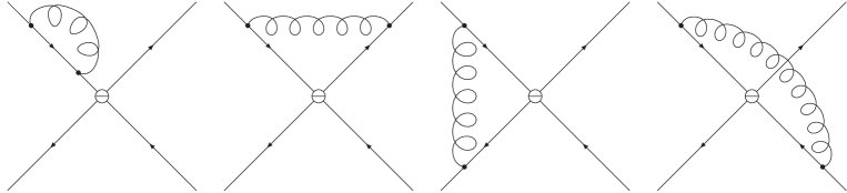
Figure 11: The diagrams for the matrix-element of ${\cal H}_{\mbox{eff}}$ at one-loop.

$$\displaystyle iC_{D}\left[\left(1+\alpha_{S}(\nu)F(q_{i})\right)S_{1}+\left(1+\alpha_{S}(\nu)F^{\prime}(q_{i})\right)S_{2}\right]$$

$$C_{D}=-C(\nu)\left(1+\frac{\alpha_{S}(\nu)}{\pi}\left[\frac{\gamma_{1}}{2}\ln\left(\frac{2q_{1}\cdot q_{2}}{\nu^{2}}\right)+r_{1}\right]\right)$$ (47)

with $S_{1}$ and $S_{2}$ the tree level matrix elements between quarks of $(\bar{s}\gamma^{\mu}d)_{L}(\bar{s}\gamma_{\mu}d)_{L}$.

We now calculate the same matrix element using $X$-boson exchange from the diagrams in Fig. 12

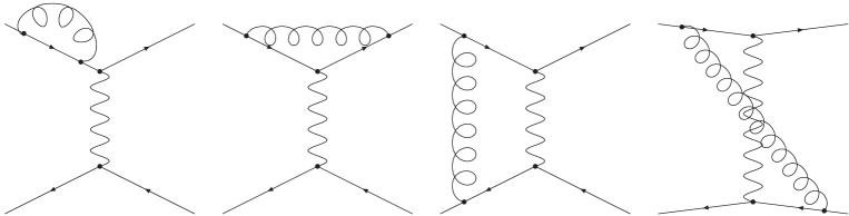
Figure 12: The same matrix element but now of $X$-boson exchange. The wiggly line is the $X$-boson.

and get

$$\displaystyle\hskip-42.67912ptiC_{C}\left[\left(1+\alpha_{S}(\mu_{C})F(q_{i})\right)S_{1}+(1+\alpha_{S}(\mu_{C})F^{\prime}(q_{i}))S_{2}\right]+{\cal O}(M_{X}^{-4})$$

$$C_{C}=\frac{-g_{X}^{2}}{M_{X}^{2}}\left(1+\frac{\alpha_{S}(\mu_{C})}{\pi}\left[\frac{\gamma_{1}}{2}\ln\left(\frac{2q_{1}\cdot q_{2}}{M_{X}^{2}}\right)+\tilde{r}_{1}\right]\right)$$ (48)

Notice that all the dependence on the external quark/gluon state in the functions $F(q_{i})$ and $F^{\prime}(q_{i})$ cancels. $r_{1}$ removes the scheme dependence and $\tilde{r}_{1}$ changes to the $X$-boson current scheme.

$g_{X}$ is now scale, scheme and external quark-gluon state independent. It still depends on the precise scheme used for the vector and axial-vector current.

The $\Delta S=1$ case is more complicated, everything becomes 10 by 10 matrices but can be found in [37]. The precise definition of the total number of $X$-bosons needed to discuss this case is

$$\displaystyle g_{1}X_{1}^{\mu}\left((\bar{s}\gamma_{\mu}d)_{L}+(\bar{u}\gamma_{\mu}u)_{L}\right)+g_{2}X_{2}^{\mu}\left((\bar{s}\gamma_{\mu}u)_{L}+(\bar{u}\gamma_{\mu}d)_{L}\right)$$

$$\displaystyle+g_{3}X_{3}^{\mu}\left((\bar{s}\gamma_{\mu}d)_{L}+\sum_{q=u,d,s}(\bar{q}\gamma_{\mu}q)_{L}\right)+g_{4}\sum_{q=u,d,s}X_{q,4}^{\mu}\left((\bar{s}\gamma_{\mu}q)_{L}+(\bar{q}\gamma_{\mu}d)_{L}\right)$$

$$\displaystyle+g_{5}X_{5}^{\mu}\left((\bar{s}\gamma_{\mu}d)_{L}+\sum_{q=u,d,s}(\bar{q}\gamma_{\mu}q)_{R}\right)+g_{6}\sum_{q=u,d,s}X_{q,6}\left((\bar{s}q)_{L}+(-2)(\bar{q}d)_{R}\right)$$

$$\displaystyle+g_{7}X_{7}^{\mu}\left((\bar{s}\gamma_{\mu}d)_{L}+\sum_{q=u,d,s}\frac{3}{2}e_{q}(\bar{q}\gamma_{\mu}q)_{R}\right)+g_{8}\sum_{q=u,d,s}X_{q,8}\left((\bar{s}q)_{L}+(-2)\frac{3}{2}e_{q}(\bar{q}d)_{R}\right)$$

$$\displaystyle+g_{9}X_{9}^{\mu}\left((\bar{s}\gamma_{\mu}d)_{L}+\sum_{q=u,d,s}\frac{3}{2}e_{q}(\bar{q}\gamma_{\mu}q)_{L}\right)+g_{10}\sum_{q=u,d,s}X_{q,10}^{\mu}\left((\bar{s}\gamma_{\mu}q)_{L}+\frac{3}{2}e_{q}(\bar{q}\gamma_{\mu}d)_{L}\right).$$ (49)

The resulting change from this correction is displayed in columns 4 and 5 of Table 3. The corrections are substantial and turn out to be in the wanted direction in all cases, surprisingly enough.

So let us summarize here the $X$-boson scheme

1. Introduce a set of fictitious gauge bosons: $X$

2. $\alpha_{S}\log({M_{X}}/{\mu})$ does not need resumming, this is not large.

3. $X$-bosons must be uncolored.

4. Only perturbative QCD and OPE have been used so far.

5. For $\hat{B}_{K}$ we need $r_{1}-\tilde{r}_{1}=-\frac{11}{12}$.

4.6.5 $X$-boson scheme matrix element: $\hat{B}_{K}$

We now need to calculate $\langle\mbox{out}|X\mbox{-exchange}|\mbox{in}\rangle$. First we do the same split in the $X$-boson momentum integral as we did for the photon

$${\int dq_{X}^{2}}\quad\Longrightarrow\quad{\int_{0}^{\mu^{2}}dq_{X}^{2}+\int_{\mu^{2}}^{\infty}dq_{X}^{2}}$$ (50)

For $q^{2}_{X}$ large, the Kaon-form-factor suppresses direct mesonic contributions by $1/q_{X}^{2}$. Large $q_{X}^{2}$ must thus flow back via quarks-gluons. The results are already suppressed by $1/N_{c}$ so we can use leading $1/N_{c}$ in this part. This part ends up replacing $\displaystyle\log\frac{\mu_{OPE}}{M_{X}}$ by $\log\frac{\mu_{OPE}}{\mu}$ such that, as it should be, $M_{X}$ has disappears completely.

For the small $q^{2}_{X}$ integral we now successively use better approximations in 3 directions:

• Low-energy that better approximates perturbative QCD

• Inclusion of quark-masses

• Inclusion of electromagnetism

The last step at present everyone only does at short-distance. Chiral Symmetry provides very strong constraints, which leads to large cancellations between various parts.

A few comments are appropriate here

• The Chiral Quark Model approach [31] does not do the identification of scales and we do not include their results. But they stressed large effects from FSI, quark-masses when factorization+small variations was the main method. See also [42].

• For some matrix-elements CHPT allows to relate them to integrals over measurable spectral functions, [43]. The remainder agrees numerically for these $B_{7},m_{\pi^{+}}^{2}-m_{\pi^{0}}^{2}$.

So the different results for $B_{K}(\mu)$ in the chiral limit are

$$B_{K}^{\chi}(\mu)=\frac{3}{4}\left[1\mbox{ (large-$N_{c}$)}-\frac{3\mu^{2}}{16\pi^{2}F_{0}^{2}}\mbox{ ($p^{2}$)}+\frac{6\mu^{4}}{16\pi^{2}F_{0}^{4}}\left(2L_{1}+5L_{2}+L_{3}+L_{9}\right)\mbox{ ($p^{4}$)}\right]$$ (51)

for CHPT[33, 35]. The ENJL model we do numerically[33, 35] and LMD gives[38]

$$B_{K}^{\chi}(\mu)=\frac{3}{4}\left\{1-\frac{1}{32\pi^{2}F_{0}^{2}}\right.\int_{0}^{\mu^{2}}dQ^{2}\left.\left(6-\sum_{i=res}\left[\frac{\alpha_{i}}{Q^{2}+M_{i}^{2}}-\frac{\alpha_{i}}{M_{i}^{2}}+\frac{\beta_{i}}{(Q^{2}+M_{i}^{2})^{2}}-\frac{\beta_{i}}{M_{i}^{4}}\right]\right)\right\}$$ (52)

$\alpha_{i}$ and $\beta_{i}$ are particular combinations of the resonance couplings. These we can now restrict by comparing CHPT and LMD,

$$\sum_{i}\frac{\alpha_{i}}{M_{i}^{4}}+\frac{\beta_{i}}{M_{i}^{6}}=\frac{24}{F_{0}^{2}}\left(2L_{1}+5L_{2}+L_{3}+L_{9}\right)\,,$$ (53)

and using short-distance constraints:

$$\sum_{i}\left(\alpha_{i}M_{i}^{2}-\beta_{i}\right)=0\quad\quad\sum_{i}\left(\frac{\alpha_{i}}{M_{i}^{2}}+\frac{\beta_{i}}{M_{i}^{4}}\right)=6\quad\quad\sum_{i}\alpha_{i}=24\pi^{2}\frac{\alpha_{S}}{\pi}F_{0}^{2}\,.$$ (54)

The last requirement is from explicitly requiring matching. The various long distance contributions in the chiral limit and in the presence of masses are shown in Fig. 14.

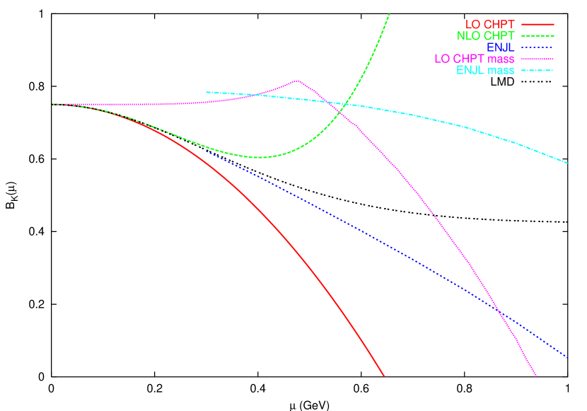
Figure 13: Comparison of the long-distance contributions to $B_{K}$ in the various approximations discussed in the text.

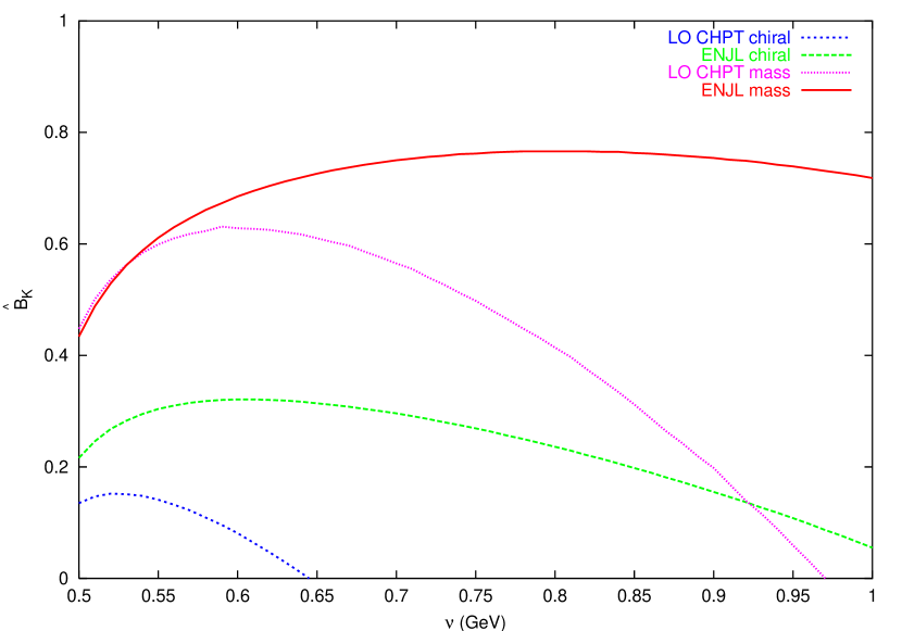
Figure 14: Using the long-distance depicted in Fig. 14 we obtain as results for $\hat{B}_{K}$ as a function of $\mu$.

Including the short-distance part leads to the results for $\hat{B}_{K}$ shown in Fig. 14 and

$$\hat{B}_{K}^{\chi} = 0.32\pm 0.06~{}(\alpha_{S})\pm 0.12~{}(\mbox{model})$$

$$\hat{B}_{K} = 0.77\pm 0.05~{}(\alpha_{S})\pm 0.05~{}(\mbox{model})\,.$$ (55)

The LMD model leads to somewhat higher but compatible results for the chiral case[38].

4.6.6 $X$-boson method results for $\Delta I=1/2$ rule and $\varepsilon^{\prime}/\varepsilon$.

We now present the results of the $X$-boson method also for the $\Delta S=1$ quantities. For other approaches I refer to the various talks given at ICHEP2000 in Osaka. The notation used below and more extensive discussions can be found in [37].

The lowest-order CHPT lagrangian for the non-leptonic $\Delta S=1$ sector is given by

$${\cal L}_{\Delta S=1} = -CF_{0}^{4}\,\left[{G_{8}}\,\mbox{tr}(\Delta_{32}u_{\mu}u^{\mu})+\,{G_{8}^{\prime}}\,\mbox{tr}(\Delta_{32}\chi_{+})\right.$$ (56)

$$+\,{G_{27}}\,t^{ijkl}\mbox{tr}(\Delta_{ij}u_{\mu}u^{\mu})\mbox{tr}(\Delta_{kl}u_{\mu}u^{\mu})\left.+{e^{2}G_{E}}F_{0}^{2}\mbox{tr}(\Delta_{32}\tilde{Q})\right]\,;$$

and contains four couplings, The various notations used are

$$U\equiv\exp\left({i\sqrt{2}\Phi/F_{0}}\right)\equiv u^{2}\,;\quad u_{\mu}\equiv iu^{\dagger}(D_{\mu}U)u\,; \chi_{+}\equiv 2B_{0}\left(u^{\dagger}{\cal M}u^{\dagger}+u{\cal M}^{\dagger}u\right)\,$$

$$\Delta_{ij}=u\lambda_{ij}u^{\dagger}\,;\quad\quad(\lambda_{ij})_{ab}=\delta_{ia}\delta_{jb}\,;\quad\quad\tilde{Q}=u^{\dagger}Qu\,; C=\frac{3G_{F}}{5\sqrt{2}}V_{ud}V_{us}^{*}$$

and are similar to the ones used by Ecker in his lectures.

Fixing the parameters from $K\to\pi\pi$ allows to predict $K\to 3\pi$ to about 30%.

In the limit $N_{c}\to\infty$ & $e\to 0$ the parameters become

$$G_{8}=G_{27}\to 1\quad G_{8}^{\prime}\,e^{2}G_{E}\to 0\,.$$ (57)

The isospin 0 and 2 amplitudes for $K\to\pi\pi$ from the above Lagrangian are

$${a_{0}} = \frac{\sqrt{6}}{9}\,CF_{0}\left[\left(9G_{8}+G_{27}\right)(m_{K}^{2}-m_{\pi}^{2})-6e^{2}G_{E}F_{0}^{2}\right]$$

$${a_{2}} = \frac{\sqrt{3}}{9}\,CF_{0}\left[10G_{27}\,(m_{K}^{2}-m_{\pi}^{2})-6e^{2}G_{E}F_{0}^{2}\right]\,.$$ (58)

The experimental values are[23, 36] Re$(G_{8})\approx 6.2$ and Re$(G_{27})\approx 0.48$ with a sizable error.

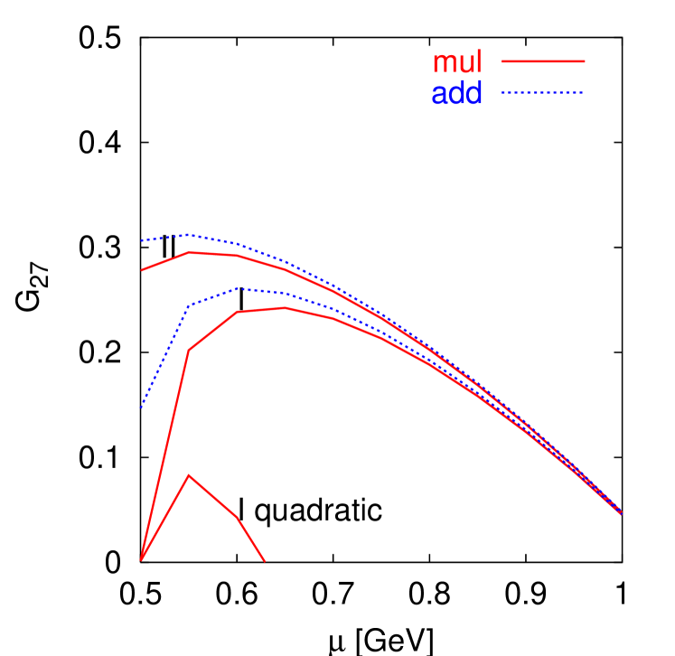
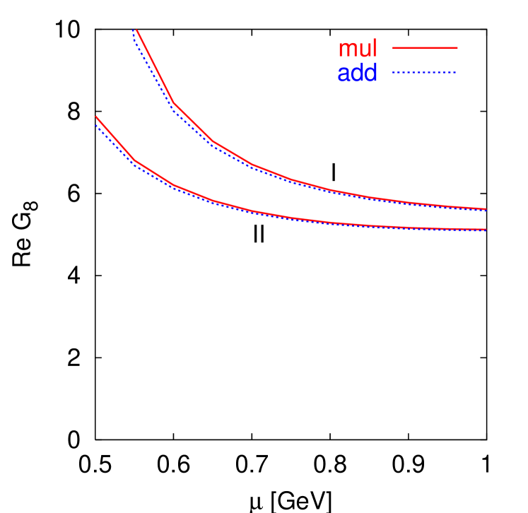
Figure 15: Results for the real part of the $\Delta S=1$ chiral lagrangian. Remember that $\mbox{Re}G_{8}^{\mbox{exp}}\approx 6.2$ and $\mbox{Re}G_{27}^{\mbox{exp}}\approx 0.48$. The labels I and II refer to two different values of $\alpha_{S}$ and mul-add to two ways of combining the various QCD corrections, differing only at higher orders.

The results obtained are shown in Fig. 15 for the real parts and in Fig. 16 for the imaginary parts. Notice that we get good matching for most quantities and good agreement with the experimental result for $G_{8}$. The bad matching for $G_{27}$ is because we have a large cancellation needed between the non-factorizable and the factorizable case to obtain matching. The 30% or so accuracy we have on the non-factorizable part leads therefore to large errors on the final result. The other quantities are not affected by such a cancellation.

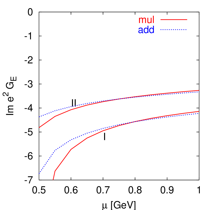
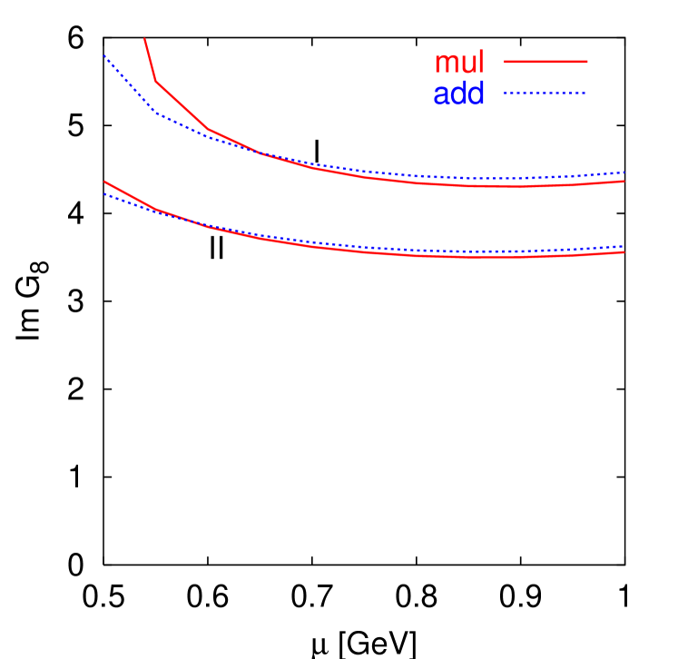
Figure 16: Results for the imaginary part of the $\Delta S=1$ chiral lagrangian.

We can now use these results to estimate $\varepsilon^{\prime}/\varepsilon$ in the chiral limit. We used $G_{27}=0.48$, $\mbox{Re}G_{8}=6.2$ and the values we obtained for the imaginary part. The same method leads to $\varepsilon$ within 10% of the experimental value. The result is shown in Fig. 17.

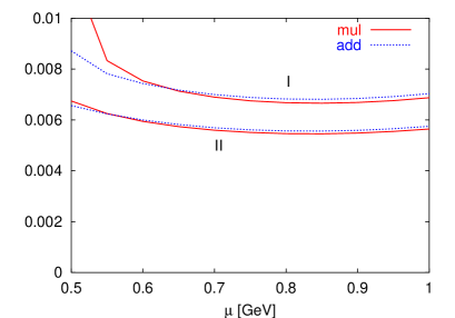
Figure 17: The results for $\varepsilon^{\prime}/\varepsilon$ in the chiral limit. Notice the quite good matching.

We can conclude that

$$\left(\frac{\varepsilon^{\prime}}{\varepsilon}\right)^{\chi}=(7.4-1.9)\cdot 10^{-3}=5.5\cdot 10^{-3}$$ (59)

and
$\bullet$ $B_{6}\approx 2.5$ not $\lesssim 1.5$
$\bullet$ $B_{8}\approx 1.3$ OK but not $B_{8}\approx B_{6}$ .

Using

$$|\varepsilon^{\prime}|\simeq\frac{1}{\sqrt{2}}\frac{\mbox{Re}\,a_{2}}{\mbox{Re}\,a_{0}}\left(-\frac{\mbox{Im}\,a_{0}}{\mbox{Re}\,a_{0}}+\frac{\mbox{Im}\,a_{2}}{\mbox{Re}\,a_{2}}\right)$$ (60)

We can now include the two main known corrections. The usual approach for final state interactions (FSI) is to take $\mbox{Re}a_{0}$, $\mbox{Re}a_{2}$ from experiment and $\mbox{Im}a_{0}$, $\mbox{Im}a_{2}$ to ${\cal O}(p^{2})$. This leads to a large suppression of the first term in (60)[42]. We evaluate both to $p^{2}$ so for us FSI act mainly on the prefactor in Eq. (60).

The main isospin breaking correction is that $\pi^{0}$,$\eta$ and $\eta^{\prime}$. This brings in a part of the large $a_{0}$ into $a_{2}$ and is thus enhanced. The effect is usually parametrized as

$$\frac{\Delta\mbox{Im}a_{2}}{\mbox{Re}a_{2}}\approx\Omega\frac{\mbox{Im}a_{0}}{\mbox{Re}a_{0}}\quad\mbox{with}\quad\Omega\approx 0.16\pm 0.03$$ (61)

where the numerical value is taken from [44].

Including the last two main corrections yields

$$\left|\frac{\varepsilon^{\prime}}{\varepsilon}\right|=(5.4-2.3)\cdot 10^{-3}=(3.1\pm??)\cdot 10^{-3}\,.$$ (62)

The size of the error is debatable but should be at least 50% given all the uncertainties involved.

5 CHPT tests in non-leptonic Kaon decays to pions

I have already shown the lowest order $\Delta S=1$ CHPT lagrangian in Eq. (56) and mentioned that this reproduces $K\to\pi\pi\pi$ to about 30% from $K\to\pi\pi$. This can now be extended to an order $p^{4}$ calculation in CHPT[23, 45]. In terms of the number of parameters and observables we have

# parameters :	$p^{2}$ :	2 (1)	$G_{8}$, $G_{27}$
	$p^{4}$ :	7(3)	($-2$ that cannot be disentangled
			from $G_{8}$, $G_{27}$)
# observables:	After isospin
$K\to 2\pi$ :	2(1)
$K\to 3\pi$ :	2(1)+1		constant in Dalitz plot
	3(1)+3		linear
	5(1)		quadratic

Phases (the +i above) of up to linear terms in the Dalitz plot might also be measurable. The numbers in brackets refer to $\Delta I=1/2$ parameters and observables only. Notice that a significant number of tests is possible. Comparison with the present data is shown in Table 4. The numbers in brackets refer to which inputs produce which predictions.

variable	$p^{2}$	$p^{4}$	experiment
$\alpha_{1}$	74	(1)input	91.71$\pm$0.32
$\beta_{1}$	$-$16.5	(2)input	$-$25.68$\pm$0.27
$\zeta_{1}$		(1)$-$0.47$\pm$0.18	$-$0.47$\pm$0.15
$\xi_{1}$		(2) $-$1.58$\pm$0.19	$-$1.51$\pm$0.30
$\alpha_{3}$	$-$4.1	(3) input	$-$7.36$\pm$0.47
$\beta_{3}$	$-$1.0	(4) input	$-$2.42$\pm$0.41
$\gamma_{3}$	1.8	(5) input	2.26$\pm$0.23
$\xi_{3}$	6	(4) 0.92$\pm$0.030	$-$0.12$\pm$0.17
$\xi_{3}^{\prime}$		(5) $-$0.033$\pm$0.077	$-$0.21$\pm$0.51
$\zeta_{3}$		(3) $-$0.0011$\pm$0.006	$-$0.21$\pm$0.08

Table 4: CHPT to order $p^{4}$ for $K\to\pi\pi\pi$. The variables refer to various measurables in the Dalitz plot. $K\to\pi\pi$ is always used as input. Numbers in brackets indicate relations.

It is important that in the future experiments tests these relations directly. At present there is satisfactory agreement with the data. Notice that new CPLEAR data decrease the errors somewhat.

CP-violation in $K\to 3\pi$ will be very difficult. The strong phases needed to interfere are just too small ([45] last reference). E.g. $\delta_{2}-\delta_{1}$ in $K_{L}\to\pi^{+}\pi^{-}\pi^{0}$ is expected to be $-0.083$ and present experiment. is only $-0.33\pm 0.29$. The CP-asymmetries expected are about $10^{-6}$ so we expect in the near future only to improve limits.

6 Kaon rare decays

The below is a summary of the summary by Isidori given at KAON99[8]. I refer there for references. Another somewhat older but more extensive review is [7] and I also found [6] useful.

Some of the processes mentioned below are tests of strong interaction physics, often in the guise of CHPT, and others are mainly SM tests.

• $\mathbf{K}^{+}\to\pi^{+}\nu\bar{\nu}$,$\mathbf{K}_{L}\to\pi^{0}\nu\bar{\nu}$ In this case the SM is strongly suppressed and dominated by short-distance physics. It is thus ideal for precision SM CKM tests and possibly new physics searches. The reason is that real and imaginary part of the amplitude are similar here in size, CKM angle suppression is counteracted by the large top-quark mass. This allows it to be dominated by $\bar{s}dZ$-Penguin and $WW$-box diagrams. The resulting

  $${\cal H}_{\mbox{eff}}=C_{\nu}(\bar{s}\gamma_{\mu}d)_{L}(\bar{\nu}\gamma^{\mu}\nu)_{L}$$ (63)

  can be hadronized using the measured matrix-element from $K_{\ell 3}$ and $\bar{\nu}\nu$ is in a CP eigenstate allowing lots of CP-tests. The main disadvantage is the extremely low predicted branching ratio of

  Neutral mode: $$(3.1\pm 1.3)\cdot 10^{-11}$$

  Charged mode: $$(8.2\pm 3.2)\cdot 10^{-11}$$ (64)

  This process will be competitive with $B$-decays in next generation of Kaon experiments.

• $\mathbf{K}_{L}\to\ell^{+}\ell^{-}$: The short-distance contribution comes from $Z$-penguin and boxes. The main uncertainty comes from the long-distance 2$\gamma$ intermediate state.

  $K_{L}\to\mu^{+}\mu^{-}$ dominated by unitary part of $K_{L}\to\gamma\gamma$, which can be taken from the branching ratio for that decay. It fits the data well.

  The long distance part of $K_{L}\to e^{+}e^{-}$ is more dependent on the contributions with off-shell photons. Here there is still work to do.

• $\mathbf{K}\to\pi\ell^{+}\ell^{-}$ The real parts can be predicted by CHPT at order $p^{4}$ from 2 parameters, it fits well. For the imaginary part there are problems with long-distance contributions from $K\to\pi\gamma\gamma$. but the CP-violating quantities are often dominated by direct part.

• $\mathbf{K}_{S}\to\gamma\gamma$ This process was a parameter-free prediction from CHPT at order $p^{4}$ from the diagrams in Fig. 19

  Figure 18: The meson-loop diagrams contributing to $K_{S}\to\gamma\gamma$. They predict the rate well.

  Figure 19: The main diagram for $K_{L}\to\gamma\gamma$ with a large uncertainty due to cancellations.

• $\mathbf{K}_{L}\to\gamma\gamma$ This decay needs more work. The underlying difficulty is that the main contribution is full of cancellations. The main diagram is shown in Fig. 19

• $\mathbf{K}_{L}\to\pi^{0}\gamma\gamma$ This process at $p^{4}$ is again a parameter-free CHPT prediction. The spectrum is well described but the rate is somewhat off. This can be explained by $p^{6}$ effects.

• $\mathbf{K}_{S}\to\pi^{0}\gamma\gamma$ This process has very similar problems as in $K_{L}\to\gamma\gamma$

• $\mathbf{K}_{L(S)}\to\gamma^{*}\gamma^{*}$ The same processes as above but with one or both photons off-shell, decaying into a $\ell^{+}\ell^{-}$-pair. These have similar questions/problems/successes as the ones with on-shell photons.

7 Conclusions

• Semi-leptonic Decays

  • CHPT is a major success and tool here.

  • These decays are the main input for $V_{ud}$ and $V_{us}$

  • In addition they provide several tests of strong interaction effects.

• $\mathbf{K}\to\pi\pi$ and $\mathbf{\overline{K^{0}}}$-$\mathbf{K}^{0}$ mixing This was the main part of the lectures. I hope I have convinced you that successful prediction is possible but more work on including extra effects and pushing down the uncertainty is obviously needed.

• $\mathbf{K}\to\pi\pi\pi$ A good test of CHPT

• Rare Decays. I only presented a very short summary of the issues.

References

- [1] B. Grinstein, Heavy Flavours, lectures at QCD2000, Benasque, Spain.
- [2] G. Ecker, Strong Interactions of Light Flavours, lectures at QCD2000, Benasque, Spain.
- [3] C. Sachrajda, QCD on the Lattice, lectures at QCD2000, Benasque, Spain.
- [4] A. J. Buras, “Weak Hamiltonian, CP violation and rare decays,” hep-ph/9806471, Les Houches lectures.
- [5] E. de Rafael, “Chiral Lagrangians and kaon CP violation,” hep-ph/9502254, TASI lectures
- [6] A. J. Buras, “CP violation and rare decays of K and B mesons,” hep-ph/9905437, Lake Louise lectures
- [7] L. Littenberg and G. Valencia, Ann. Rev. Nucl. Part. Sci. 43 (1993) 729 [hep-ph/9303225].
- [8] G. Isidori, “Standard model vs new physics in rare kaon decays,” hep-ph/9908399, talk KAON99
- [9] T. van Ritbergen and R. G. Stuart, Nucl. Phys. B564 (2000) 343 [hep-ph/9904240].
- [10] D. E. Groom et al., Eur. Phys. J. C15 (2000) 1.
- [11] C. Caso et al., Eur. Phys. J. C3 (1998) 1.
- [12] W. S. Woolcock, Mod. Phys. Lett. A6(1991)2579.
- [13] H. Leutwyler and M. Roos, Z. Phys. C25 (1984) 91.
- [14] M. Knecht et al. and G. Amoros et al., work in progress.
- [15] J. Bijnens, G. Colangelo, G. Ecker and J. Gasser, hep-ph/9411311 in 2nd DAPHNE Physics Handbook.
- [16] J. Bijnens, hep-ph/9907514, talk KAON99.
- [17] A. Afanasev and W. W. Buck, “Form factors of kaon semileptonic decays,” hep-ph/9607445.
- [18] G. Amoroset al.,Nucl. Phys. B568 (2000) 319 [hep-ph/9907264].
- [19] M. Knecht et al.,Eur. Phys. J. C12 (2000) 469 [hep-ph/9909284].
- [20] G. Amoros, J. Bijnens and P. Talavera, Phys. Lett. B480 (2000) 71 [hep-ph/9912398]; Nucl. Phys. B585 (2000) 293 [hep-ph/0003258].
- [21] J. Bijnens, G. Ecker and J. Gasser, Nucl. Phys. B396 (1993) 81 [hep-ph/9209261].
- [22] L. Ametller et al.,Phys. Lett. B303 (1993) 140 [hep-ph/9302219].
- [23] J. Kambor, J. Missimer and D. Wyler, Phys. Lett. B261 (1991) 496.
- [24] J. H. Christenson, J. W. Cronin, V. L. Fitch and R. Turlay, Phys. Rev. Lett. 13 (1964) 138.
- [25] A. Alavi-Harati et al. (KTeV), Phys. Rev. Lett. 83 (1999) 22; A. Ceccucci, CERN Particle Physics Seminar (29 February 2000) www.cern.ch/NA48; V. Fanti et al. (NA48), Phys. Lett. B465 (1999) 335; H. Burkhart et al. (NA31), Phys. Lett. B206 (1988) 169; G.D. Barr et al. (NA31), Phys. Lett. B317 (1993) 233; L.K. Gibbons et al. (E731), Phys. Rev. Lett. 70 (1993) 1203
- [26] M. K. Gaillard and B. W. Lee, Phys. Rev. Lett. 33 (1974) 108; G. Altarelli and L. Maiani, Phys. Lett. B52 (1974) 351; A. I. Vainshtein, V. I. Zakharov and M. A. Shifman, JETP Lett. 22 (1975) 55; F. J. Gilman and M. B. Wise, Phys. Rev. D20 (1979) 2392; B. Guberina and R. D. Peccei, Nucl. Phys. B163 (1980) 289; J. Bijnens and M. B. Wise, Phys. Lett. B137 (1984) 245; M. Lusignoli, Nucl. Phys. B325 (1989) 33; J. M. Flynn and L. Randall, Phys. Lett. B224 (1989) 221.
- [27] A. J. Buras and P. H. Weisz, Nucl. Phys. B333 (1990) 66. A. J. Buras, M. Jamin, E. Lautenbacher and P. H. Weisz, Nucl. Phys. B370 (1992) 69, Addendum-ibid. B375 (1992) 501; A. J. Buras, M. Jamin and M. E. Lautenbacher, Nucl. Phys. B400 (1993) 75 [hep-ph/9211321]. A. J. Buras et al.,Nucl. Phys. B400 (1993) 37 [hep-ph/9211304]; M. Ciuchini et al.,Nucl. Phys. B415 (1994) 403 [hep-ph/9304257].
- [28] S. Herrlich and U. Nierste, Nucl. Phys. B476 (1996) 27 [hep-ph/9604330].
- [29] W. A. Bardeen et al.,Phys. Lett. B192 (1987) 138; Nucl. Phys. B293 (1987) 787.
- [30] T. Hambye, G. O. Köhler, E. A. Paschos, P. H. Soldan and W. A. Bardeen, Phys. Rev. D58 (1998) 014017 [hep-ph/9802300]; T. Hambye, G. O. Köhler and P. H. Soldan, Eur. Phys. J. C10 (1999) 271 [hep-ph/9902334]; T. Hambye, G. O. Köhler, E. A. Paschos and P. H. Soldan, Nucl. Phys. B564 (2000) 391 [hep-ph/9906434].
- [31] A. Pich and E. de Rafael, Nucl. Phys. B358 (1991) 311; V. Antonelli, S. Bertolini, J. O. Eeg, M. Fabbrichesi and E. I. Lashin, Nucl. Phys. B469 (1996) 143 [hep-ph/9511255]; V. Antonelli, S. Bertolini, M. Fabbrichesi and E. I. Lashin, Nucl. Phys. B469 (1996) 181 [hep-ph/9511341]; S. Bertolini, J. O. Eeg and M. Fabbrichesi, Nucl. Phys. B476 (1996) 225 [hep-ph/9512356]; S. Bertolini, J. O. Eeg, M. Fabbrichesi and E. I. Lashin, Nucl. Phys. B514 (1998) 93 [hep-ph/9706260]; S. Bertolini, J. O. Eeg and M. Fabbrichesi, hep-ph/0002234.
- [32] J. Bijnens, C. Bruno and E. de Rafael, Nucl. Phys. B390 (1993) 501 [hep-ph/9206236]; J. Bijnens, Phys. Rept. 265 (1996) 369 [hep-ph/9502335] and references therein.
- [33] J. Bijnens and J. Prades, Phys. Lett. B342 (1995) 331 [hep-ph/9409255]; Nucl. Phys. B444 (1995) 523 [hep-ph/9502363].
- [34] J. Bijnens and J. Prades, JHEP 9901 (1999) 023 [hep-ph/9811472].
- [35] J. Bijnens and J. Prades, JHEP 0001 (2000) 002 [hep-ph/9911392].
- [36] J. Bijnens, E. Pallante and J. Prades, Nucl. Phys. B521 (1998) 305 [hep-ph/9801326].
- [37] J. Bijnens and J. Prades, JHEP 0006 (2000) 035 [hep-ph/0005189].
- [38] M. Knecht, S. Peris and E. de Rafael, Phys. Lett. B457 (1999) 227 [hep-ph/9812471]; S. Peris and E. de Rafael, Phys. Lett. B490 (2000) 213 [hep-ph/0006146].
- [39] Hai-Yang Cheng, talk at ICHEP 2000, Osaka, Japan, 27 Jul - 2 Aug 2000, hep-ph/0008284 and references therein.
- [40] W. A. Bardeen, J. Bijnens and J. M. Gerard, Phys. Rev. Lett. 62 (1989) 1343; J. Bijnens, Phys. Lett. B306 (1993) 343 [hep-ph/9302217].
- [41] J. Bijnens and J. Prades, Nucl. Phys. B490 (1997) 239 [hep-ph/9610360]
- [42] E. Pallante and A. Pich, Phys. Rev. Lett. 84 (2000) 2568 [hep-ph/9911233]; hep-ph/0007208.
- [43] J. F. Donoghue and E. Golowich, Phys. Lett. B478 (2000) 172 [hep-ph/9911309].
- [44] G. Ecker, G. Muller, H. Neufeld and A. Pich, Phys. Lett. B477 (2000) 88 [hep-ph/9912264].
- [45] J. Kambor, J. F. Donoghue, B. R. Holstein, J. Missimer and D. Wyler, Phys. Rev. Lett. 68 (1992) 1818; G. D’Ambrosio, G. Isidori, A. Pugliese and N. Paver, Phys. Rev. D50 (1994) 5767 [hep-ph/9403235].