Thermalisation of inhomogeneous quantum scalar fields in 1+1D

Abstract

Using an improved version of the Hartree approximation, allowing for ensembles of inhomogeneous configurations, we show in a $\lambda\phi^{4}$ theory, that initially the system thermalises with a Bose-Einstein distribution. For later times and larger couplings we see deviations.

Introduction

In many parts of high energy physics like early universe physics and heavy ion collisions one wants to follow quantum field systems in time. Typical phenomena include reheating after inflation: after a phase of parametric resonance most energy is in a small part of the spectrum, a non-thermal initial condition.

In order to study these systems and to describe phase transitions and thermal fluctuations between classical minima, non-perturbative approximation schemes are needed. Examples of high temperature approximations, that have been used successfully are the classical approximationgrigo ; aarts and the Hartree or gaussian approximationmihai . The latter assumes a gaussian density matrix, such that all information is contained in the 1- and 2-point functions, higher point functions can be factorised using Wick’s theorem.

Inhomogeneous Hartree ensemble

Instead of the commonly used Hartree approximation, which has a spatially constant mean field we used an improved version, allowing for inhomogeneous configurations. We studied this approximation in a scalar $\phi^{4}$ theory in $1+1$ dimensions:

$${\mathcal{L}}=-\frac{1}{2}\partial_{\mu}\hat{\phi}\partial^{\mu}\hat{\phi}-\frac{1}{2}\mu^{2}\hat{\phi}^{2}-\frac{1}{4}\lambda\hat{\phi}^{4}.$$ (1)

In the gaussian approximation we can expand the operator field in mode functions:

$$\hat{\phi}(x,t)=\phi(x,t)+\sum_{\alpha}\,\left(\hat{a}_{\alpha}f_{\alpha}(x,t)+\hat{a}_{\alpha}^{\dagger}f_{\alpha}^{*}(x,t)\right),$$ (2)

where the time-independent $\hat{a}_{\alpha}$ and $\hat{a}_{\alpha}^{\dagger}$ satisfy the usual commutation relations. We can choose them such that:

$$\langle\hat{a}_{\alpha}^{\dagger}\hat{a}_{\alpha}\rangle\equiv n_{\alpha}^{0}.$$ (3)

For a free thermal system the $n^{0}_{\alpha}$ have a Bose-Einstein form and the $f_{\alpha}(x,t)$ are plane waves, with suitable normalisation.

The Heisenberg equations of motions in the gaussian approximation become:

$$\mbox{[}\partial_{t}^{2}-\triangle+\mu^{2}+\phantom{3}\lambda\phi^{2}(x,t)+3\lambda\Sigma(x,t)\mbox{]} \phi(x,t) =0,$$ (4)

$$\mbox{[}\partial_{t}^{2}-\triangle+\mu^{2}+3\lambda\phi^{2}(x,t)+3\lambda\Sigma(x,t)\mbox{]} f_{\alpha}(x,t) =0,$$ (5)

$$\Sigma(x,t)=\sum_{\alpha}\,|f_{\alpha}(x,t)|^{2}\,(2n_{\alpha}^{0}+1).$$ (6)

We mention that there exists an effective Hamiltonian which leads to the above equations, suggesting that in the end the system will equilibrate classically according to this $H_{\rm eff}$. But we hope that this has a timescale much larger than that of all interesting processes.

Initial conditions

We need to specify the initial fields and their conjugate momenta, which together with the $n_{\alpha}^{0}$ specifies an initial gaussian density matrix. By averaging over different runs with different initial conditions we can build non-gaussian density matrices, allowing for much more general initial conditions. Only the time evolution is evaluated with gaussian density matrices.

We will take the mean field in its zero-temperature minimum, with all energy in a few of its momentum modes, like after parametric resonance:

$$\phi(x,0)=v\qquad\textrm{and}\qquad\dot{\phi}(x,0)=A\sum_{j=1}^{j_{\rm max}}\cos\left(2\pi j\frac{x}{L}-\psi_{j}\right),$$ (7)

where the $\psi_{j}$’s are random phases and $2\pi j_{\rm max}/L$ is of the order $m$. We will average over several runs, typically 10-20.

For simplicity we will take the quantum modes equal to the zero-temperature vacuum form:

$$n_{\alpha}^{0}=0,\qquad f_{k}(x,0)=\frac{{\rm e}^{ikx}}{\sqrt{2\omega_{k}L}},\qquad\dot{f}_{k}(x,0)=-\frac{i\omega_{k}{\rm e}^{ikx}}{\sqrt{2\omega_{k}L}},$$ (8)

with $\omega_{k}=\sqrt{m^{2}+k^{2}}$, $m$ chosen as the zero-temperature mass and $L$ the size of the system. To put the system on a computer we discretise it on a space-time lattice. In the limit of (spatial) lattice spacing $a$ to zero, the mode sum $\Sigma$ occurring in the equations of motion is logarithmically diverging, but this can be fixed by a simple mass renormalisation: $\mu^{2}\rightarrow\mu_{\rm ren}^{2}\equiv\mu^{2}-\frac{3\lambda}{4\pi}\log(\lambda a^{2})$.

Thermalisation

If $\lambda$ is small and the system is not too far from equilibrium the interaction of the mode functions with the typically inhomogeneous mean field can be viewed as scattering of particles via the mean field. Because of this scattering they will hopefully thermalise according to a thermal – i.e. Bose-Einstein – distribution.

To check this, a definition of particle number is needed. For a free thermal system the 2-point functions read:

$$\langle\hat{\phi}_{x}\hat{\phi}_{y}\rangle_{\rm conn}=\sum_{k}\frac{1}{\omega_{k}}\,\frac{n_{k}+\frac{1}{2}}{L}\,{\rm e}^{ik(x-y)},\qquad\langle\hat{\pi}_{x}\hat{\pi}_{y}\rangle_{\rm conn}=\sum_{k}\omega_{k}\,\frac{n_{k}+\frac{1}{2}}{L}\,{\rm e}^{ik(x-y)}.$$ (9)

We want to define an $n_{k}$ and $\omega_{k}$ in a similar way as Eq. 9. This can be done by coarsening the measured 2-point functions over the initial conditions, a time interval, and space.

Numerical results

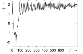
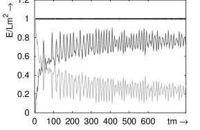
Figure 1: Left: time dependence of the average mean field. Right: the energy densities for the same run: total (straight line at 1), mean field (starting at total energy), and modes.

In Fig. 1 we plotted for a typical run ($256$ lattice points, size $Lm=32$, $\lambda/m^{2}=1/12$) the spatial averages of the mean field and the energy densities as a function of time. We see that the energy, initially completely in the mean field, is going to the modes with a timescale of the order 100 in mass units. The total energy is conserved up to a few percent. The energy staying in the mean field – around 20% – is much more than expected from classical equipartition: around $1/256$ for $256$ mode functions.

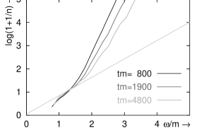
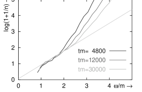
Figure 2: The particle numbers for smaller and longer times. For a true BE $\log(1+1/n)=\beta\omega$. The straight line is a BE fit at the latest time plotted.

Fig. 2 shows a plot of the calculated particle numbers obtained after averaging over whole space, approximately 5 oscillation periods and 10 configurations. On the left the situation is plotted at shorter times, on the right at larger times. We see that starting at low momenta, a Bose-Einstein distribution is emerging. Only the zero mode is showing deviations.

Runs at twice this energy density show very similar results, but with faster thermalisation. At large times deviations from the straight line BE’s start to show up, which we interpret as signs of classical equipartition. For strong coupling or after a long times we see the emergence of an offset, which might be a chemical potential following from approximate particle conservation.

We finally mention checks with different kinds of initial conditions (not presented here), which also show thermalisation according to a Bose-Einstein distribution.

Conclusion

Using our Hartree ensemble approximation with inhomogeneous mean fields, we find thermalisation according to a Bose-Einstein distribution, starting in the low momentum modes. The time-scales heavily depend on the size of the coupling and the energy density.

Signs of classical equilibration occur only at timescales much larger than that for the onset of the Bose-Einstein thermalisation, so even if they will prevent the BE thermalisation to reach arbitrary high values of $\omega$, they do not influence processes with an intermediate timescale.

An extension to higher dimensions is wanted but numerically demanding. A possible way out is a reduction of the number of mode functions.

A more elaborate discussion of these simulations is in preparation.

References

- (1) Grigoriev, D., and Rubakov, V., Nucl. Phys. B299, 67-78 (1988)
-
(2)
Aarts, G., Bonini, G.F., and Wetterich, C.,
hep-ph/0007357 -
(3)
Mihaila, B., Athan, T., Cooper, F., Dawson, J., and Habib, S.,
hep-ph/0003105