October 19, 2000 LBNL-46980

IASSNS-AST-00/55

hep-ph/0010231

On the Evolution of the Neutrino State inside the Sun

Alexander Friedland

Theoretical Physics Group
Ernest Orlando Lawrence Berkeley National Laboratory
University of California, Berkeley, California 94720

and

School of Natural Sciences, Institute for Advanced Study
Einstein Drive, Princeton, NJ 08540

We reexamine the conventional physical description of the neutrino evolution inside the Sun. We point out that the traditional resonance condition has physical meaning only in the limit of small values of the neutrino mixing angle, $\theta\ll 1$. For large values of $\theta$, the resonance condition specifies neither the point of the maximal violation of adiabaticity in the nonadiabatic case, nor the point where the flavor conversion occurs at the maximal rate in the adiabatic case. The corresponding correct conditions, valid for all values of $\theta$ including $\theta>\pi/4$, are presented. An adiabaticity condition valid for all values of $\theta$ is also described. The results of accurate numerical computations of the level jumping probability in the Sun are presented. These calculations cover a wide range of $\Delta m^{2}$, from the vacuum oscillation region to the region where the standard exponential approximation is good. A convenient empirical parametrization of these results in terms of elementary functions is given. The matter effects in the so-called “quasi-vacuum oscillation regime” are discussed. Finally, it is shown how the known analytical results for the exponential, $1/x$, and linear matter distributions can be simply obtained from the formula for the hyperbolic tangent profile. An explicit formula for the jumping probability for the distribution $N_{e}\propto(\coth(x/l)\pm 1)$ is obtained.

1 Introduction

The solar neutrino problem (SNP) is a discrepancy between the measured values of the solar neutrino flux at different energies [1, 2, 3, 4, 5] and the corresponding predictions of the Standard Solar Model (SSM) [6]. Not only is the observed flux suppressed, compared to the SSM predictions, but, if the data from the Homestake experiment are correct, the degree of suppression varies with energy. The leading explanation of this phenomenon is that neutrinos have small masses and the mass and flavor bases in the lepton sector are not aligned, just like in the quark sector. The resulting neutrino oscillations convert some of the solar electron neutrinos into another neutrino species.

Neutrino oscillation solutions to the SNP have traditionally been divided into the so-called Mikheyev-Smirnov-Wolfenstein (MSW) solutions [7, 8, 9] and the vacuum oscillation (VO) solutions, according to the physical mechanism responsible for the neutrino flavor conversion in each case. In the MSW case the conversion is caused by neutrino interactions with the solar (and Earth’s) matter, while in the VO case it is due to long-wavelength neutrino oscillations in vacuum between the Sun and the Earth. Over time, it has become a tradition to treat the two cases completely separately, showing results in separate plots (see, for example, [10, 11]) and using different input formulas and different codes.

Justifying such a complete separation, however, requires a careful analysis of the magnitude of the solar matter effects and the degree of decoherence of vacuum oscillations. The separation assumption has been recently reexamined by the author [12] and it has been found that the solar matter effects are nonnegligible for the vacuum oscillation solutions with $\Delta m^{2}\mathrel{\mathchoice{\lower 3.0pt\vbox{\halign{$\m@th\displaystyle\hfill#\hfil$\cr>\crcr\sim\crcr}}}{\lower 3.0pt\vbox{\halign{$\m@th\textstyle\hfill#\hfil$\cr>\crcr\sim\crcr}}}{\lower 3.0pt\vbox{\halign{$\m@th\scriptstyle\hfill#\hfil$\cr>\crcr\sim\crcr}}}{\lower 3.0pt\vbox{\halign{$\m@th\scriptscriptstyle\hfill#\hfil$\cr>\crcr\sim\crcr}}}}5\times 10^{-10}$ eV². This conclusion has been subsequently verified by other authors [13, 14, 15], and the term quasi-vacuum oscillations (QVO) has been coined to refer to the region where both effects influence the neutrino survival probability [13].

It must be mentioned that the experimental situation has changed since the QVO solutions were first introduced. At the time, the most preferred part of the VO solutions was in the region $\Delta m^{2}<10^{-10}$ eV². The latest Super-Kamiokande spectrum data, however, disfavors a large fraction of the vacuum oscillation region, roughly $2\times 10^{-11}$ eV² $<\Delta m^{2}<4\times 10^{-10}$ eV² [16, 15]. At the same time, the solutions with $\Delta m^{2}>4\times 10^{-10}$ eV², i. e. the QVO solutions, remain allowed.

Prior to [12], the VO solutions had always been studied in the range of the neutrino mixing angle $0\leq\theta\leq\pi/4$ for a fixed sign of $\Delta m^{2}$. When matter effects are included, however, this only covers a half of the full parameter space. To cover the full space, one can either (i) keep $\theta$ in the range $0\leq\theta\leq\pi/4$ and consider both signs of $\Delta m^{2}$, or (ii) fix the sign of $\Delta m^{2}$ and vary $\theta$ from $0$ to $\pi/2$. We advocate the second option as a better physical choice, because it makes manifest the continuity of physics around the maximal mixing [17, 18].

The parametrization $0<\theta<\pi/2$ requires one to reexamine the choice of a variable for plots, because the traditional variable $\sin^{2}2\theta$ is not suitable for this purpose [17]. While either $\theta$ or $\sin^{2}\theta$ would be adequate for plotting only the QVO region, neither choice allows one to take a global view of the neutrino parameter space and show all solutions, including the SMA and (quasi)vacuum oscillation solutions, on the same plot [18]. A particularly convenient choice turns out to be $\tan^{2}\theta$ on the logarithmic scale, first used in [19] to describe 3-family MSW oscillations. In addition to covering the range $0<\theta<\pi/2$, it also does not introduce any unphysical singularity around $\theta=\pi/4$ (unlike the traditional $\sin^{2}2\theta$, see [17]) and makes it easy to see where in the vacuum oscillation region the evolution in the Sun becomes completely nonadiabatic (points $\theta$ and $\pi/2-\theta$ become equivalent, so that solutions become symmetric with respect to the $\theta=\pi/4$ line).

In the first part of this paper we address several conceptual questions that arise in the analysis of the solar matter effects and become particularly apparent for the values of the mixing angle $\theta\geq\pi/4$. To introduce these questions, it is useful to first summarize the basic mechanism of the neutrino evolution in the Sun. Inside the Sun, because of the changing electron density, the eigenstates of the instantaneous Hamiltonian change along the neutrino trajectory. For $\Delta m^{2}/E_{\nu}\ll 10^{-5}$ eV²/MeV the neutrino is produced almost completely in the heavy eigenstate. If the parameters $\Delta m^{2}/E_{\nu}$ and $\theta$ are such that the neutrino remains in the heavy eigenstate as it travels to the solar surface (adiabatic evolution), there are no subsequent vacuum oscillations. To oscillate in vacuum, as a necessary condition, the neutrino must at some radius in the Sun “jump” into the superposition of the heavy ($\nu_{2}$) and light ($\nu_{1}$) mass eigenstates. Conventional VO regime is realized when this “jumping” is extremely nonadiabatic (preserving flavor), in which case the neutrino exits the Sun as $\cos\theta|\nu_{1}\rangle+e^{i\phi}\sin\theta|\nu_{2}\rangle$. In the QVO regime the neutrino still partially jumps in the $\nu_{1}$ eigenstate, but with a smaller amplitude.

The obvious questions one would like to answer are:

• What physical criteria determine whether the neutrino evolution is adiabatic or not?

• At what radius in the Sun does the nonadiabatic “jumping” between the eigenstates of the instantaneous Hamiltonian take place?

The traditional wisdom is that one should analyze the density profile around the so-called resonance point, i.e., the point where the difference of the eigenvalues of the instantaneous Hamiltonian is minimal and the local value of the mixing angle is $\theta_{m}=\pi/4$ (see, e.g., [20, 21, 22, 23, 24, 25, 26]). This, however, clearly needs to be modified for large mixing angles. In particular, for $\theta>\pi/4$ the resonance, defined in this way, simply does not exist. We will show how this contradiction is resolved in Section 2.2. In Section 2.3 we formulate the adiabaticity condition that, unlike the standard result, remains valid for $\theta\mathrel{\mathchoice{\lower 3.0pt\vbox{\halign{$\m@th\displaystyle\hfill#\hfil$\cr>\crcr\sim\crcr}}}{\lower 3.0pt\vbox{\halign{$\m@th\textstyle\hfill#\hfil$\cr>\crcr\sim\crcr}}}{\lower 3.0pt\vbox{\halign{$\m@th\scriptstyle\hfill#\hfil$\cr>\crcr\sim\crcr}}}{\lower 3.0pt\vbox{\halign{$\m@th\scriptscriptstyle\hfill#\hfil$\cr>\crcr\sim\crcr}}}}\pi/4$.

In Section 3 we present the results of numerical calculations of the jumping probability $P_{c}$ for the neutrino propagating in the realistic solar profile. The calculations are carried out for a wide range of $\Delta m^{2}$ and $\tan^{2}\theta$, from the VO region to the region where the exponential density approximation is valid. We show how the adiabaticity prescription of Section 2.3 applies to this case. We also give a simple empirical prescription on how to compute $P_{c}$ in this range of the parameters in terms of only elementary functions. Such an empirical parametrization of the numerical results can be helpful if one would like to be able to quickly estimate the value of $P_{c}$ anywhere in the range in question without having to solve the differential equation each time.

In Section 3.2, we discuss what happens in the transitional region between the adiabatic and nonadiabatic regimes (QVO). In particular, we determine what part of the solar electron density profile is primarily responsible for the matter effects in this region.

Finally, in Section 4 we comment on the four known exact analytical solutions for the neutrino jumping probability $P_{c}$. Such solutions have been found for the linear, exponential, $1/r$, and the hyperbolic tangent matter density profiles. A natural question to ask is whether these profiles have something in common that makes finding exact solutions possible. Using the formulation of the evolution equations introduced in Section 2, we show that all four results are not independent and that, given the formula for the hyperbolic tangent profile, one can very simply obtain the other three solutions. As an added benefit, we obtain an exact expression for the density distribution $N_{e}\propto(\coth(x/l)\pm 1)$.

2 Physics of the nonadiabatic neutrino evolution

2.1 Review of the oscillation formalism

For completeness, we begin by summarizing the well-known basic formalism for neutrino oscillations in matter. In the simplest case, when the mixing is between $\nu_{e}$ and another active neutrino species, the evolution of the neutrino state is determined by four parameters: the mass-squared splitting between the neutrino mass eigenstates $\Delta m^{2}\equiv m_{2}^{2}-m_{1}^{2}$, the neutrino mixing angle $\theta$, the neutrino energy $E_{\nu}$, and the electron number density $N_{e}$ of the medium. One has to solve the Schrödinger equation $id\phi/dt=H\phi$, where $\phi=(\phi_{e},\phi_{\mu})^{T}$ is the state vector made up of the electron neutrino and the muon neutrino. The Hamiltonian $H$ is given by [7]

$$H=\mbox{const}+\left(\begin{array}[]{cc}A-\Delta\cos 2\theta&\Delta\sin 2\theta\\ \Delta\sin 2\theta&\Delta\cos 2\theta-A\end{array}\right),$$ (2.3)

where $\Delta\equiv\Delta m^{2}/(4E_{\nu})$ and $A\equiv\sqrt{2}G_{F}N_{e}/2$. The constant in the Hamiltonian is irrelevant for the study of oscillations and will be omitted from now on. The time variable $t$ may be replaced by the distance traveled $x$, since the solar neutrinos are ultrarelativistic.

For a constant electron number density $N_{e}$ the Hamiltonian can be trivially diagonalized, $H^{\prime}=VHV^{\dagger}=\mbox{diag}(-\Delta_{m},+\Delta_{m})$, where

$$\Delta_{m}=\sqrt{(A-\Delta\cos 2\theta)^{2}+(\Delta\sin 2\theta)^{2}}=\sqrt{A^{2}-2A\Delta\cos 2\theta+\Delta^{2}}.$$ (2.4)

In terms of $\Delta_{m}$, the Hamiltonian (2.3) can be rewritten as

$$H=\left(\begin{array}[]{rr}-\Delta_{m}\cos 2\theta_{m}&\Delta_{m}\sin 2\theta_{m}\\ \Delta_{m}\sin 2\theta_{m}&\Delta_{m}\cos 2\theta_{m}\end{array}\right),$$ (2.7)

where $\theta_{m}$ is the mixing angle in matter. The rotation matrix $V$ is given by

$$V=\left(\begin{array}[]{rr}\cos\theta_{m}&-\sin\theta_{m}\\ \sin\theta_{m}&\cos\theta_{m}\end{array}\right).$$ (2.10)

The parameters $\Delta_{m}$ and $\theta_{m}$ are related to the original parameters in the Hamiltonian (2.3) as follows

$$\Delta_{m}\sin 2\theta_{m} = \Delta\sin 2\theta,$$ (2.11)

$$\Delta_{m}\cos 2\theta_{m} = \Delta\cos 2\theta-A,$$ (2.12)

$$\tan 2\theta_{m} = \frac{\Delta\sin 2\theta}{\Delta\cos 2\theta-A}.$$ (2.13)

We will always label the light mass eigenstate by $\nu_{1}$ and the heavy one by $\nu_{2}$. Since one can redefine the phases of $\nu_{e,\mu}$ and $\nu_{1,2}$, it is easy to see that in this convention the physical range of the mixing angle is $0\leq\theta\leq\pi/2$ [18, 17].

As long as $N_{e}(x)$ is constant, the time evolution of the mass eigenstates is particularly simple. Each of the two mass eigenstates evolves only by a phase: $|\nu_{1}(t)\rangle=|\nu_{1}(0)\rangle\exp(i\Delta_{m}t)$, $|\nu_{2}(t)\rangle=|\nu_{2}(0)\rangle\exp(-i\Delta_{m}t)$. If at time $t=0$ the neutrino state is a linear combination $a|\nu_{1}(0)\rangle+b|\nu_{2}(0)\rangle$, the absolute values of the coefficients $a$ and $b$ do not change with time, i.e., the probability for the neutrino to “jump” from one Hamiltonian eigenstate to another, $P_{c}\equiv|a(t=+\infty)|^{2}-|a(t=0)|^{2}$, is trivially zero.

Consider next the case of a varying electron density. In this case, in general, one can no longer diagonalize the Hamiltonian in Eq. (2.3). However, one can still speak of the eigenstates of the instantaneous Hamiltonian (henceforth, “the matter mass eigenstates”), and define the jumping probability between those states. It turns out that if the electron density changes sufficiently slowly along the neutrino trajectory (to be quantified later), the jumping probability vanishes, just like in the constant density case. This is known as the adiabatic evolution. At the same time, when the density changes abruptly, the jumping probability is clearly nonzero. In particular, if the neutrino crosses a step–function density discontinuity, the flavor state does not have any time to evolve, while the mass basis in matter instantaneously rotates. It is easy to see that in this situation, known as the extreme nonadiabatic evolution, the jumping probability is given by

$$P_{c}^{\rm NA}=\sin^{2}(\theta^{\rm before}-\theta^{\rm after}).$$ (2.14)

In general, for a monotonically varying density $P_{c}$ lies between 0 and $P_{c}^{\rm NA}$.

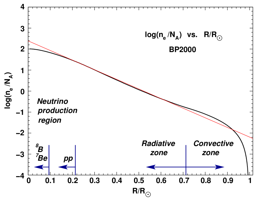
Figure 1: The electron number density profile of the Sun according to the BP2000 standard solar model.

In this paper we are concerned with the evolution of solar neutrinos. The electron number density inside the Sun, $N_{e}$, falls off as a function of the distance from the center $r$ as shown in Fig. 1 [6]. In the range $0.15R_{\odot}\mathrel{\mathchoice{\lower 3.0pt\vbox{\halign{$\m@th\displaystyle\hfill#\hfil$\cr<\crcr\sim\crcr}}}{\lower 3.0pt\vbox{\halign{$\m@th\textstyle\hfill#\hfil$\cr<\crcr\sim\crcr}}}{\lower 3.0pt\vbox{\halign{$\m@th\scriptstyle\hfill#\hfil$\cr<\crcr\sim\crcr}}}{\lower 3.0pt\vbox{\halign{$\m@th\scriptscriptstyle\hfill#\hfil$\cr<\crcr\sim\crcr}}}}r\mathrel{\mathchoice{\lower 3.0pt\vbox{\halign{$\m@th\displaystyle\hfill#\hfil$\cr<\crcr\sim\crcr}}}{\lower 3.0pt\vbox{\halign{$\m@th\textstyle\hfill#\hfil$\cr<\crcr\sim\crcr}}}{\lower 3.0pt\vbox{\halign{$\m@th\scriptstyle\hfill#\hfil$\cr<\crcr\sim\crcr}}}{\lower 3.0pt\vbox{\halign{$\m@th\scriptscriptstyle\hfill#\hfil$\cr<\crcr\sim\crcr}}}}0.65R_{\odot}$ the profile can be approximated very well by an exponential $N_{e}(r)\propto\exp(-r/r_{0})$, with $r_{0}=R_{\odot}/10.54=6.60\times 10^{4}$ km (shown by a straight line in the Figure). However, in the convective zone of the Sun and also in the core where the neutrinos are produced the profile deviates rather significantly from exponential.

In order to study the jumping probability between the matter mass eigenstates it is convenient to change to the basis these states define. Substituting in the Schrödinger equation $\phi=V^{\dagger}\psi$, $\psi\equiv(\psi_{1},\psi_{2})$, we get

$$i\frac{d}{dx}(V^{\dagger}\psi) = HV^{\dagger}\psi,$$

$$i\frac{d\psi}{dx} = VHV^{\dagger}\psi-iV\frac{dV^{\dagger}}{dx}\psi.$$ (2.15)

Since $VHV^{\dagger}=\mbox{diag}(-\Delta_{m},+\Delta_{m})$ and from Eq. (2.10)

$$V\frac{dV^{\dagger}}{dx}=\left(\begin{array}[]{rr}0&1\\ -1&0\end{array}\right)\frac{d\theta_{m}}{dx},$$

we obtain the desired evolution equation in the basis of the matter mass eigenstates [20]

$$\frac{d}{dx}\left(\begin{array}[]{c}\psi_{1}\\ \psi_{2}\end{array}\right)=\left(\begin{array}[]{cc}i\Delta_{m}&-d\theta_{m}/dx\\ d\theta_{m}/dx&-i\Delta_{m}\end{array}\right)\left(\begin{array}[]{c}\psi_{1}\\ \psi_{2}\end{array}\right).$$ (2.22)

The steps outlined so far are standard in the treatment of the MSW effect. We will next make an extra step that will prove very helpful for the subsequent analysis, particularly in Section 4. Namely, we will choose $\theta_{m}$ instead of $x$ as an independent variable. So long as the density varies monotonically, such a change is one-to-one. Eq. (2.22) becomes

$$\frac{d}{d\theta_{m}}\left(\begin{array}[]{c}\psi_{1}\\ \psi_{2}\end{array}\right)=\left(\begin{array}[]{cc}i\Delta_{m}/\dot{\theta}_{m}&-1\\ 1&-i\Delta_{m}/\dot{\theta}_{m}\end{array}\right)\left(\begin{array}[]{c}\psi_{1}\\ \psi_{2}\end{array}\right).$$ (2.29)

Here $\Delta_{m}$ and $\dot{\theta}_{m}\equiv d\theta_{m}/dx$ can both be expressed in terms of $\theta_{m}$ using the following relationships

$$\dot{\theta}_{m} = \frac{\sin^{2}2\theta_{m}}{2\Delta\sin 2\theta}\frac{dA}{dx},$$ (2.30)

$$\frac{\Delta_{m}}{\dot{\theta}_{m}} = \frac{2\Delta^{2}\sin^{2}2\theta}{\sin^{3}2\theta_{m}}\frac{1}{dA/dx},$$ (2.31)

$$A = \frac{\Delta\sin(2\theta_{m}-2\theta)}{\sin 2\theta_{m}},$$ (2.32)

which follow directly from Eqs. (2.11-2.13). For instance, for the infinitely extending exponential profile $A(x)=A_{0}\exp(-x/r_{0})$ the derivative is $dA(x)/dx=-A(x)/r_{0}$ and so

$$\frac{\Delta_{m}}{\dot{\theta}_{m}}=-\frac{2\Delta r_{0}\sin^{2}2\theta}{\sin^{2}2\theta_{m}\sin(2\theta_{m}-2\theta)}.$$ (2.33)

The angle $\theta_{m}$ varies from its value at the production point $\theta_{\odot}$ to its vacuum value $\theta$. For the infinite exponential profile we have $\theta_{\odot}\rightarrow\pi/2$. Notice that the quantity $\Delta_{m}/\dot{\theta}_{m}$ in Eq. (2.33) is singular when $\theta_{m}$ approaches either of its limiting values, as should be expected.

\psfrag{theta_m}{{\large$\theta_{m}$}}\psfrag{Dmthetadot}{{\large$|\Delta_{m}/\dot{\theta}_{m}|$}}\psfrag{1}{{\large 1}}\psfrag{1.5}{{\large 1.5}}\psfrag{1.4}{{\large 1.4}}\psfrag{1.3}{{\large 1.3}}\psfrag{1.2}{{\large 1.2}}\psfrag{1.1}{{\large 1.1}}\psfrag{0.9}{{\large 0.9}}\psfrag{0.8}{{\large 0.8}}\psfrag{10}{{\large 10}}\psfrag{8}{{\large 8}}\psfrag{6}{{\large 6}}\psfrag{4}{{\large 4}}\psfrag{2}{{\large 2}}\psfrag{Exponential}{{\large Exponential}}\psfrag{BP2000}{{\large BP2000}}\includegraphics[angle={0},width=433.62pt]{Dmthetadot2.eps}

Figure 2: The quantity $|\Delta_{m}/\dot{\theta}_{m}|$ as a function of $\theta_{m}$ for the exponential profile $A(x)\propto\exp(-x/r_{0})$ (solid line) and BP2000 solar profile (dashed line) for $\theta=\pi/4$, $\Delta=10^{-9}$ eV²/MeV.

The shape of the function $|\Delta_{m}/\dot{\theta}_{m}|$ for $\theta=\pi/4$ and $\Delta=10^{-9}$ eV²/MeV for the idealized exponential profile is shown in Fig. 2 by the solid curve. The value of $r_{0}$ was chosen to be $R_{\odot}/10.54$, the slope of the best fit line in Fig. 1. The dashed curve in the Figure shows the same quantity for the realistic BP2000 solar profile for the same values of $\theta$ and $\Delta$. It is important to keep in mind that the two curves change qualitatively differently as one changes $\Delta$. While the exponential curve just scales by an overall factor, the BP2000 curve also changes its shape, approaching the shape of the (rescaled) solid curve for sufficiently large values of $\Delta$.

2.2 Modification of the notion of resonance for large $\theta$.

We are ready to address the questions posed in the introduction. A convenient starting point is the evolution equation in the form of Eq. (2.29). Neutrino is produced in the $\nu_{e}$ state, which corresponds to $(\cos\theta_{\odot},\sin\theta_{\odot})$ in the matter mass basis. To simplify the presentation, we shall consider the values of $\Delta\ll 10^{-5}$ eV²/MeV, so that at the production point $\Delta\ll A_{\odot}$, and hence $(\cos\theta_{\odot},\sin\theta_{\odot})\rightarrow(0,1)$.

The evolution equation can be easily solved in the two limiting cases. If the off-diagonal elements can be neglected, the evolution is adiabatic, i.e., $|\psi_{2}(\theta_{m})|^{2}$ remains constant. If, on the other hand, for almost the entire interval between $\theta_{\odot}$ and $\theta$ the diagonal terms can be neglected, the solution is

$$\psi(\theta) = \exp\left[\int_{\theta_{\odot}}^{\theta}d\theta_{m}\left(\begin{array}[]{rr}0&-1\\ 1&0\end{array}\right)\right]\psi(\theta_{\odot})$$ (2.36)

$$= \left(\begin{array}[]{rr}\cos(\theta-\theta_{\odot})&-\sin(\theta-\theta_{\odot})\\ \sin(\theta-\theta_{\odot})&\cos(\theta-\theta_{\odot})\end{array}\right)\psi(\theta_{\odot}).$$ (2.39)

This limit corresponds to the extreme nonadiabatic case. The corresponding jumping probability equals $P_{c}=\sin^{2}(\theta_{\odot}-\theta)=\cos^{2}\theta$, in agreement with Eq. (2.14).

Returning for a moment to the physical $x$–space, we note that no jumping between the mass eigenstates occurs either in the solar core [7] or in vacuum. The nonadiabatic evolution takes place in a localized region, with a center at the point of “the maximal violation of adiabaticity”. Our goal next is to establish the location of this point.

Conventional wisdom says that the adiabaticity condition is violated maximally at the resonance point

$$A=\Delta\cos 2\theta,$$ (2.40)

where the separation between the energy levels is minimal and $\theta_{m}=\pi/4$. This assertion can be found in the early papers [21, 22, 20, 27], as well as in numerous subsequent reviews on the subject, e.g. [24, 25, 26]. However, in all these papers it is assumed either explicitly or implicitly that the vacuum mixing angle $\theta$ is small. It is easy to see that for a large value of the mixing angle the use of the condition in Eq. (2.40) leads to a contradiction.

For small $\theta$, Eq. (2.40) is satisfied in a layer in the Sun where the density is $A(x)\simeq\Delta$. As the value of $\theta$ increases, Eq. (2.40) predicts that the resonance occurs at lower and lower electron density until, as $\theta$ approaches $\pi/4$, it moves off to infinity. It is not obvious how to interpret the last result, as it is physically clear that no level jumping can occur at infinity where neutrinos undergo ordinary vacuum oscillations. The difficulty is even more obvious when $\theta>\pi/4$, in which case the resonance simply never occurs. At the same time, as already mentioned, in the extreme nonadiabatic regime the level jumping probability is nonzero for any value of $\theta$ and varies smoothly around $\theta=\pi/4$, $P_{c}=\cos^{2}\theta$.

The resolution to this apparent paradox is very simple. As Eq. (2.29) suggests, adiabaticity is maximally violated at the minimum of $|\Delta_{m}/\dot{\theta}_{m}|$ ([20, 27]). It is easy to see, however, that the minimum of $|\Delta_{m}/\dot{\theta}_{m}|$ in general does not reduce to the condition of Eq. (2.40). This can be explicitly seen on the example of the infinite exponential density distribution. Differentiating Eq. (2.33), one finds that the minimum occurs when

$$\cot(2\theta_{m}-2\theta)+2\cot(2\theta_{m})=0,$$ (2.41)

or

$$A=\Delta\frac{\cos 2\theta+\sqrt{8+\cos^{2}2\theta}}{4}.$$ (2.42)

Unlike Eq. (2.40), Eq. (2.42) states there is a nonadiabatic part of the neutrino trajectory for all physical values of $\theta$, including $\theta\geq\pi/4$. While both equations for small $\theta$ predict that jumping between the local mass eigenstates occurs around $A=\Delta$, Eq. (2.42) states that for maximal mixing it occurs around $A=\Delta/\sqrt{2}$, not at infinity, and for $\theta$ close to $\pi/2$ it happens around $A=\Delta/2$, all physically sensible results.

\psfrag{psi}{{\large$|\psi_{2}|^{2}$}}\psfrag{r, 10^6 km}{{\large$x$, $\times 10^{6}$ km}}\psfrag{pi/3}{{\large$\theta=\pi/3$}}\psfrag{pi/4}{{\large$\theta=\pi/4$}}\psfrag{pi/6}{{\large$\theta=\pi/6$}}\psfrag{pi/60}{{\large$\theta=\pi/60$}}\psfrag{1}{{\large 1}}\psfrag{1.4}{{\large 1.4}}\psfrag{1.2}{{\large 1.2}}\psfrag{1.0}{{\large 1.0}}\psfrag{0.8}{{\large 0.8}}\psfrag{0.6}{{\large 0.6}}\psfrag{0.4}{{\large 0.4}}\psfrag{0.2}{{\large 0.2}}\includegraphics[angle={0},width=409.77406pt]{transition.eps}

Figure 3: Neutrino state evolution in the case of the infinite exponential density profile for $\Delta m^{2}/E_{\nu}=10^{-9}$ eV²/MeV. The plot shows the probability of finding the neutrino in the heavy matter mass eigenstate $\nu_{2}$ as a function of position $x$, for four different values of the vacuum mixing angle. The points of the maximal violation of adiabaticity, as predicted by Eq. (2.42), are marked.

The situation is illustrated in Fig. 3, which shows the probability of finding the neutrino in the heavy mass state $\nu_{2}$ as a function of the distance $x$. The parameters of the exponential were taken from the fit line in Fig. 1 and $\Delta m^{2}/E_{\nu}=10^{-9}$ eV²/MeV. Three large values of the mixing angle ($\theta=\pi/6,\pi/4,\mbox{ and }\pi/3$) and one small value ($\theta=\pi/60$) were chosen. The dashed lines and dots mark the points where adiabaticity is maximally violated, as predicted by Eq. (2.42). One can see that the partial jumping into the light mass eigenstate in all four cases indeed occurs around the marked points.

It is instructive to analyze each of the factors $\Delta_{m}$ and $1/\dot{\theta}_{m}$ separately. The first one indeed has a minimum at the traditional resonance point $\theta_{m}=\pi/4$ (corresponding to Eq. (2.40)) or, if $\theta>\pi/4$, at the endpoint $\theta_{m}=\theta$. The second one, however, has a minimum at a point which is, in general, different from the resonance. This minimum exists for all values of $\theta$, including $\theta>\pi/4$. In the case of the exponential profile, it is located at

$$\theta_{m}=\pi/4+\theta/2,$$ (2.43)

or halfway between $\theta$ and $\theta_{\odot}=\pi/2$. The corresponding value of the density at that point is

$$A=\Delta.$$ (2.44)

This coincides with the resonance condition for $\theta\ll 1$ and that is why the standard resonance description works very well in this limit. In general, however, the minimum of the product function lies somewhere between $\pi/4$ and $\pi/4+\theta/2$ (or $\theta$ and $\pi/4+\theta/2$, if $\theta>\pi/4$).

It is also worth mentioning that Eqs. (2.43) and (2.44) represent an important condition in the case of the adiabatic evolution. Namely, they specify a point where the rate of rotation of the mass basis with respect to the flavor basis is maximal, which in the adiabatic case can be interpreted as a point where the flavor composition of the neutrino state changes at the fastest rate. This shows that for large $\theta$ Eq. (2.40) not only does not describe the point of the maximal violation of adiabaticity in the nonadiabatic regime, but also does not specify the point where the flavor conversion occurs at the maximal rate in the adiabatic regime.

To summarize, Eq. (2.40) can only be used in the small angle limit. Even in that case one should be careful applying it for certain purposes. Note, for example, that Eqs. (2.40) and (2.42) have different Taylor series expansion around $\theta=0$,

$$A \simeq \Delta(1-2\theta^{2}/3)\;\;\;\;\mbox{ for Eq. (\ref{eq:minexp2})},$$

$$A \simeq \Delta(1-2\theta^{2})\;\;\;\;\;\;\;\>\mbox{ for Eq. (\ref{eq:resonance})}.$$

Thus, even at small $\theta$, Eq. (2.40) fails to predict how the point of maximal nonadiabaticity shifts as a function of $\theta$.

The belief that jumping between the matter mass eigenstates occurs at the resonance for all values of $\theta$ might have been one of the reasons for the tradition to treat separately the cases of $\theta<\pi/4$ and $\theta>\pi/4$, obscuring the fact that physics is completely continuous across $\theta=\pi/4$. Over the years, it has caused some unfortunate confusions, as exemplified by the flawed criticism of the results of [12] in [29]. It was probably the principal reason why the correct expression for the electron neutrino survival probability in the $\theta>\pi/4$ part of the QVO region was not given until recently [17, 12] (c.f. Eq. (6) in [19]).

One important application of Eq. (2.42) is the determination of the phase of vacuum oscillations on the Earth [30, 31]. If jumping between matter mass eigenstates indeed occurred at the resonance (2.40), one would expect that in the canonical vacuum oscillation formula

$$P=1-\sin^{2}2\theta\sin^{2}\left(1.27\frac{\Delta m^{2}L}{E}+\delta_{\rm res}\right),$$ (2.45)

the residual phase $\delta_{\rm res}$ would be minimized when the distance $L$ was measured from the resonance in the Sun. Ref. [31] indeed begins with this assumption, but after presenting the resulting formulas notes that the residual phase is much smaller if $L$ is instead measured from the layer where $A=\Delta$, not $A=\Delta\cos 2\theta$. It is unfortunate that this important observation has not received proper attention and was not further developed in the subsequent literature. The preceding discussion shows that this result is not just a mathematical coincidence, but has a simple physical explanation.

Finally, it is important to discuss at what density the adiabaticity is maximally violated in the case of the realistic solar profile. Qualitatively, it is not difficult to anticipate the changes to Eq. (2.42) in this case.

• For sufficiently large $\Delta$, the adiabaticity is maximally violated in the radiative zone, entirely within the exponential part of the profile, so that Eq. (2.42) directly applies.

• For small $\Delta$, the nonadiabatic part of the trajectory lies close to the surface of the Sun where the profile falls off rather rapidly. While for small $\theta$ the minimum of $\Delta_{m}/\dot{\theta}_{m}$ should still, of course, occur at $A=\Delta$, for large angles it is shifted to values of $A$ somewhat lower than those predicted by Eq. (2.42). The evolution in the latter case will be discussed in more detail in Section 3.2.

• For $\Delta$ in the intermediate range, the jumping occurs near the bottom of the convective zone where the density falls off somewhat slower than in the exponential part. There the value of the ratio $A/\Delta$ at large $\theta$ should increase compared to Eq. (2.42).

These qualitative expectations are supported by the results of numerical calculations presented in Fig. 4, where the ratio $A/\Delta$ at the point of minimal $\Delta_{m}/\dot{\theta}_{m}$ is plotted as function of $\theta$. The three curves shown correspond to the values of $\Delta$ in the three different regimes: $\Delta=2\times 10^{-6}$ eV²/MeV (curve 1), $\Delta=7\times 10^{-8}$ eV²/MeV (curve 2), and $\Delta=1\times 10^{-8}$ eV²/MeV (curve 3). The numerical studies of the BP2000 solar profile are presented in Section 3.

\psfrag{theta_m}{{\large$\theta_{m}$}}\psfrag{dm/theta_m}{{\large$A(x)/\Delta$ at min of $\Delta_{m}/\dot{\theta}_{m}$ }}\psfrag{0}{{\large$0$}}\psfrag{1}{{\large$1$}}\psfrag{2}{{\large$2$}}\psfrag{3}{{\large$3$}}\psfrag{0.2}{{\large$0.2$}}\psfrag{0.4}{{\large$0.4$}}\psfrag{0.6}{{\large$0.6$}}\psfrag{0.8}{{\large$0.8$}}\psfrag{0.25}{{\large$0.25$}}\psfrag{0.5}{{\large$0.5$}}\psfrag{0.75}{{\large$0.75$}}\psfrag{1.25}{{\large$1.25$}}\psfrag{1.5}{{\large$1.5$}}\includegraphics[angle={0},width=433.62pt]{bp2000jumping.eps}

Figure 4: The value of the ratio $A(x)/\Delta$ at the minimum of $\Delta_{m}/\dot{\theta}_{m}$ computed for the realistic solar density profile (BP2000). The curves correspond to $\Delta=2\times 10^{-6}$ eV²/MeV (curve 1), $\Delta=7\times 10^{-8}$ eV²/MeV (curve 2), and $\Delta=1\times 10^{-8}$ eV²/MeV (curve 3).

2.3 Adiabaticity condition for large $\theta$.

We now turn to formulating the adiabaticity condition that is valid for all, and not just small, values of the mixing angle $\theta$. At first sight it appears that for the evolution to be adiabatic it is simply enough to require that the diagonal elements in Eq.(2.29) be larger than the off-diagonal ones. This condition becomes most critical at the point where the adiabaticity is maximally violated. Since traditionally this point has been identified with the resonance, a commonly cited condition is [20]

$$|\Delta_{m}/\dot{\theta}_{m}|_{\theta_{m}=\pi/4}\gg 1.$$ (2.46)

Since we have shown that the point of the maximal violation of adiabaticity in general does not coincide with the resonance, Eq. (2.46) clearly needs to be modified for large mixing angles. Superficially, the problem appears easy to fix: one should evaluate the left hand side at a value of $\theta_{m}$ close to the true point of the maximal violation of adiabaticity. In the case of the exponential profile, this point would be given by the solution of Eq. (2.41). For the purpose of an estimate, we can approximate it by the point halfway between $\theta$ and $\pi/2$ (see Eq. (2.43)),

$$|\Delta_{m}/\dot{\theta}_{m}|_{\theta_{m}\sim\pi/4+\theta/2}\gg 1.$$ (2.47)

This condition, however, still turns out to be inadequate for large values of $\theta$. To obtain the correct condition, one has to analyze the problem more carefully.

The key is to express the information contained in the system of two evolution equations in a single equation. Such an equation can be easily written for the ratio $s\equiv\psi_{1}/\psi_{2}$. From Eq. (2.29) it follows that $s$ obeys the following first order equation

$$\frac{ds}{d\theta_{m}}=2i\frac{\Delta_{m}}{\dot{\theta}_{m}}s-(s^{2}+1).$$ (2.48)

\psfrag{tan}{{\large$\tan^{2}\theta$}}\psfrag{dm2}{{\large$\Delta m^{2}/E_{\nu}$, (eV${}^{2}$/MeV)}}\psfrag{0}{{\large$1$}}\psfrag{1}{{\large$10$}}\psfrag{2}{{\large$10^{2}$}}\psfrag{3}{{\large$10^{3}$}}\psfrag{-1}{{\large$10^{-1}$}}\psfrag{-2}{{\large$10^{-2}$}}\psfrag{-3}{{\large$10^{-3}$}}\psfrag{7}{{\large$10^{-7}$}}\psfrag{8}{{\large$10^{-8}$}}\psfrag{9}{{\large$10^{-9}$}}\psfrag{10}{{\large$10^{-10}$}}\psfrag{11}{{\large$10^{-11}$}}\psfrag{Pc=0.9}{{\large$P_{c}=0.9$}}\psfrag{0.7}{{\large$0.7$}}\psfrag{0.5}{{\large$0.5$}}\psfrag{0.3}{{\large$0.3$}}\psfrag{0.1}{{\large$0.1$}}\psfrag{0.01}{{\large$10^{-2}$}}\psfrag{0.001}{{\large$10^{-3}$}}\psfrag{Adiabatic}{{\Large Adiabatic}}\psfrag{Nonadiabatic}{{\Large Nonadiabatic}}\psfrag{Eq1}{{\large Eq. (\ref{eq:oldad0})}}\psfrag{Eq2}{{\large Eq. (\ref{eq:oldad})}}\psfrag{Eq3}{{\large Eq. (\ref{eq:adiabaticity})}}\includegraphics[angle={0},width=433.62pt]{adiabaticity3.eps}

Figure 5: The boundary between the adiabatic and nonadiabatic regions in the case of the exponential profile, as predicted by Eq. (2.46), Eq. (2.47), and Eq. (2.50). The dashed curves show the contours of constant $P_{c}$. For large angles Eq. (2.50) provides a better description of the boundary.

It is easy to see that by neglecting appropriate terms on the right hand side one obtains both the adiabatic and nonadiabatic limits. The adiabatic limit corresponds to neglecting the terms in parentheses, while the extreme nonadiabatic limit is obtained if one neglects the first term on the right. In the second case the solution is $s=\cot(\theta_{m})$. Thus, the self consistent condition to have the extreme nonadiabatic solution is $2|\Delta_{m}/\dot{\theta}_{m}s|\ll(s^{2}+1)$, with $s=\cot(\theta_{m})$, $\theta_{m}=\pi/4+\theta/2$. In the opposite limit, the evolution is adiabatic. Thus, we obtain the adiabaticity condition

$$|\Delta_{m}/\dot{\theta}_{m}|_{\theta_{m}\sim\pi/4+\theta/2}\gg(\tan(\pi/4+\theta/2)+\cot(\pi/4+\theta/2))/2,$$ (2.49)

or, upon simplification,

$$\cos\theta|\Delta_{m}/\dot{\theta}_{m}|_{\theta_{m}\sim\pi/4+\theta/2}\gg 1.$$ (2.50)

Notice, that all three conditions, Eqs. (2.46), (2.47), and (2.50) agree in the small angle limit. For large angles, however, especially for $\theta\mathrel{\mathchoice{\lower 3.0pt\vbox{\halign{$\m@th\displaystyle\hfill#\hfil$\cr>\crcr\sim\crcr}}}{\lower 3.0pt\vbox{\halign{$\m@th\textstyle\hfill#\hfil$\cr>\crcr\sim\crcr}}}{\lower 3.0pt\vbox{\halign{$\m@th\scriptstyle\hfill#\hfil$\cr>\crcr\sim\crcr}}}{\lower 3.0pt\vbox{\halign{$\m@th\scriptscriptstyle\hfill#\hfil$\cr>\crcr\sim\crcr}}}}\pi/4$, they give very different predictions and only Eq. (2.50) is the correct one.

Let us demonstrate this on the example of the infinite exponential profile. In this case the exact analytical solution is known [32, 33] (see also [34]),

$$P_{c}=\frac{e^{\gamma\cos^{2}\theta}-1}{e^{\gamma}-1}.$$ (2.51)

Eq. (2.51) has two regimes. For small mixing angles, the formula reduces to $P_{c}=\exp(-\gamma\sin^{2}\theta)$, so the evolution is nonadiabatic when $\gamma\theta^{2}=4\pi r_{0}\Delta\theta^{2}\ll 1$. By contract, for $\theta\mathrel{\mathchoice{\lower 3.0pt\vbox{\halign{$\m@th\displaystyle\hfill#\hfil$\cr>\crcr\sim\crcr}}}{\lower 3.0pt\vbox{\halign{$\m@th\textstyle\hfill#\hfil$\cr>\crcr\sim\crcr}}}{\lower 3.0pt\vbox{\halign{$\m@th\scriptstyle\hfill#\hfil$\cr>\crcr\sim\crcr}}}{\lower 3.0pt\vbox{\halign{$\m@th\scriptscriptstyle\hfill#\hfil$\cr>\crcr\sim\crcr}}}}\pi/4$ and $\gamma\gg 1$ the numerator is always much smaller than the denominator. The transition between the adiabatic and nonadiabatic regimes now occurs when $\gamma\sim 1$, with a weak dependence on $\theta$.

Let us see if Eq. (2.50) correctly captures this behavior. Using Eq. (2.33) we obtain

$$8\Delta r_{0}\sin^{2}\theta\gg 1.$$ (2.52)

Fig. 5 shows the contour of $8\Delta r_{0}\sin^{2}\theta=1$ computed for $r_{0}=R_{\odot}/10.54$ (solid line). For comparison, the dash-dotted curves shows the corresponding prediction of Eqs. (2.46) and (2.47). The dashed curves are the contours of constant $P_{c}$ computed using Eq. (2.51). It is clear from the Figure that the description of Eq. (2.50) is correct not only for small $\theta$, but also for $\theta\mathrel{\mathchoice{\lower 3.0pt\vbox{\halign{$\m@th\displaystyle\hfill#\hfil$\cr>\crcr\sim\crcr}}}{\lower 3.0pt\vbox{\halign{$\m@th\textstyle\hfill#\hfil$\cr>\crcr\sim\crcr}}}{\lower 3.0pt\vbox{\halign{$\m@th\scriptstyle\hfill#\hfil$\cr>\crcr\sim\crcr}}}{\lower 3.0pt\vbox{\halign{$\m@th\scriptscriptstyle\hfill#\hfil$\cr>\crcr\sim\crcr}}}}\pi/4$. The transition from adiabaticity to nonadiabaticity for $\theta\mathrel{\mathchoice{\lower 3.0pt\vbox{\halign{$\m@th\displaystyle\hfill#\hfil$\cr>\crcr\sim\crcr}}}{\lower 3.0pt\vbox{\halign{$\m@th\textstyle\hfill#\hfil$\cr>\crcr\sim\crcr}}}{\lower 3.0pt\vbox{\halign{$\m@th\scriptstyle\hfill#\hfil$\cr>\crcr\sim\crcr}}}{\lower 3.0pt\vbox{\halign{$\m@th\scriptscriptstyle\hfill#\hfil$\cr>\crcr\sim\crcr}}}}\pi/4$ occurs for $\Delta m^{2}/E_{\nu}\sim 10^{-9}$ eV²/MeV, precisely where $\gamma\sim 1$.

The true usefulness of Eq. (2.50) is not so much in being able to explain the physics behind the known analytical solution as it is in being able to make predictions for a variety of new density profiles, provided those profiles are sufficiently smooth. Such an analysis, however, would be beyond the scope of this paper. The question we do want to address is what Eq. (2.50) predicts for the realistic solar density profile. It turns out that for large mixing angles and the values of $\Delta$ that yield nonadiabatic evolution the nonadiabatic jumping takes place mostly in the convective zone, where the density profile deviates from the exponential, and so one can no longer rely on (2.51) to get the shape of the boundary between the adiabatic and nonadiabatic regions. Eq. (2.50) nonetheless works quite well. The corresponding numerical results are presented next.

3 Calculations for the realistic solar profile

3.1 Numerical calculations of the jumping probability

In this Section we present the results of numerical computation of the jumping probability $P_{c}$ with the realistic (BP2000) solar density profile. In practice, ultimately, one would like to compute expected event rates at various experiments, and for that one needs to know the solar neutrino survival probability $P(\nu_{e}\rightarrow\nu_{e})$. It is, however, quite straightforward to show that, for a given neutrino energy, the survival probability is given by

$$P(\nu_{e}\rightarrow\nu_{e})=P_{1}\cos^{2}\theta+(1-P_{1})\sin^{2}\theta$$ (3.1)

$$- \sqrt{P_{c}(1-P_{c})}\cos 2\theta_{\odot}\sin 2\theta\cos\left(2.54\frac{\Delta m^{2}}{E}L+\delta\right),$$

where $P_{1}=P_{c}\sin^{2}\theta_{\odot}+(1-P_{c})\cos^{2}\theta_{\odot}$ [18]. Thus, the problem of finding $P(\nu_{e}\rightarrow\nu_{e})$ reduces to finding the jumping probability $P_{c}$.

The quantity $P_{c}$ can be found analytically in several limiting regimes. For $\Delta m^{2}/E_{\nu}\mathrel{\mathchoice{\lower 3.0pt\vbox{\halign{$\m@th\displaystyle\hfill#\hfil$\cr>\crcr\sim\crcr}}}{\lower 3.0pt\vbox{\halign{$\m@th\textstyle\hfill#\hfil$\cr>\crcr\sim\crcr}}}{\lower 3.0pt\vbox{\halign{$\m@th\scriptstyle\hfill#\hfil$\cr>\crcr\sim\crcr}}}{\lower 3.0pt\vbox{\halign{$\m@th\scriptscriptstyle\hfill#\hfil$\cr>\crcr\sim\crcr}}}}10^{-7}$ eV²/MeV the condition of Eq. (2.42) is satisfied well inside the Sun where the profile is exponential with $r_{0}=R_{\odot}/10.54$. Hence, in this case the jumping probability should be adequately described by Eq. (2.51).

The second regime is $\theta\ll 1$, in which case the standard resonance description applies and, importantly, the resonance is very narrow. As a result, the jumping probability can be adequately described by the analytical formula for a linear density profile, $P_{c}=\exp(-\pi\Delta^{2}\sin^{2}2\theta|dA(x)/dx|_{A=\Delta}^{-1})$ (Eq. (4.1) of Sect. 4). The contours of constant $P_{c}$ in this regime are expected to follow the behavior of the changing slope of the BP2000 density profile shown in Fig. 1.

The third regime is the region of small $\Delta$ and large $\theta$. As already discussed, for $\Delta\rightarrow 0$ the evolution becomes extremely nonadiabatic, i. e., $P_{c}\rightarrow\cos^{2}\theta$. For $\Delta m^{2}/E_{\nu}\sim 10^{-9}$ eV²/MeV we have the so-called quasivacuum oscillation region. It was shown in [12] that for $\Delta m^{2}/E_{\nu}\mathrel{\mathchoice{\lower 3.0pt\vbox{\halign{$\m@th\displaystyle\hfill#\hfil$\cr<\crcr\sim\crcr}}}{\lower 3.0pt\vbox{\halign{$\m@th\textstyle\hfill#\hfil$\cr<\crcr\sim\crcr}}}{\lower 3.0pt\vbox{\halign{$\m@th\scriptstyle\hfill#\hfil$\cr<\crcr\sim\crcr}}}{\lower 3.0pt\vbox{\halign{$\m@th\scriptscriptstyle\hfill#\hfil$\cr<\crcr\sim\crcr}}}}5\times 10^{-9}$ eV²/MeV Eq. (2.51) provides a good fit to numerical calculations, provided one takes $r_{0}=R_{\odot}/18.4$. This region will be discussed in more detail in Section 3.2.

We next present numerical results for $P_{c}$ that cover the entire range between these regimes. We numerically solve Eq. (2.48) on a grid of points in the range $10^{-3}<\tan^{2}\theta<10$, $10^{-11}\mbox{ eV}^{2}/\mbox{MeV}<\Delta m^{2}/E_{\nu}<2\times 10^{-7}\mbox{ eV}^{2}/\mbox{MeV}$. Notice that, while the same result would be obtained by solving the system of equations in Eq. (2.22), Eq. (2.48) requires significantly less computer time. Indeed, Eq. (2.22) contains four real functions (real and imaginary parts of $\psi_{1}$ and $\psi_{2}$), but only two of them are independent, since $|\psi_{1}|^{2}+|\psi_{2}|^{2}=1$ and the overall phase has no physical meaning.

The resulting contours of constant $P_{c}$ are shown in Fig. 6 by solid curves. All the features anticipated in the discussion above are clearly present.

We can now test the validity of the adiabaticity criterion introduced in the previous Section (Eq. (2.50)). The shaded region in Fig. 1 corresponds to $\cos\theta|\Delta_{m}/\dot{\theta}_{m}|_{\theta_{m}=\pi/4+\theta/2}\geq 1$. As one can see by comparing its shape with that of the contours of constant $P_{c}$, the criterion in question indeed describes the adiabatic region quite well, even for $\theta>\pi/4$.

\psfrag{tan^2 theta}{{\Large$\tan^{2}\theta$}}\psfrag{dm^2/E}{{\Large$\Delta m^{2}/E$ (eV${}^{2}$/MeV)}}\psfrag{-7}{{\large$10^{-7}$}}\psfrag{-8}{{\large$10^{-8}$}}\psfrag{-9}{{\large$10^{-9}$}}\psfrag{-10}{{\large$10^{-10}$}}\psfrag{-11}{{\large$10^{-11}$}}\psfrag{1}{{\large$1$}}\psfrag{10}{{\large$10$}}\psfrag{0.1 }{{\large$0.1$}}\psfrag{0.01}{{\large$0.01$}}\includegraphics[angle={0},width=433.62pt]{empiricalfit.eps}

Figure 6: Contours of constant level jumping probability $P_{c}$. The solid line represent the result of numerical calculations using the BP2000 solar profile. The dashed lines illustrate a possible empirical fit using only elementary functions (Eq. (3.2)).

For practical calculations it is convenient to have a simple expression involving only elementary functions that provides a satisfactory means of estimating $P_{c}$ without having to solve the differential equation each time. We can construct such a purely empirical fit function by taking Eq. (2.51) as a starting point. Since for both large and small values of $\Delta m^{2}/E_{\nu}$ one can use Eq. (2.51) with the appropriate values of $r_{0}$, we can modify Eq. (2.51) by making $r_{0}$ a function of $\Delta m^{2}/E_{\nu}$, smoothly interpolating between $R_{\odot}/10.54$ and $R_{\odot}/18.4$,

$$r_{0}(\Delta m^{2}/E_{\nu})=\frac{R_{\odot}}{10.54}\left[0.75\left(\frac{1}{\pi}\arctan[-10(a+8)]+\frac{1}{2}\right)+1\right]^{-1},$$ (3.2)

where $a=\log_{10}[(\Delta m^{2}/E_{\nu})/({\rm eV}^{2}/{\rm MeV})]$. This provides an adequate fit for both $\Delta m^{2}/E_{\nu}\mathrel{\mathchoice{\lower 3.0pt\vbox{\halign{$\m@th\displaystyle\hfill#\hfil$\cr<\crcr\sim\crcr}}}{\lower 3.0pt\vbox{\halign{$\m@th\textstyle\hfill#\hfil$\cr<\crcr\sim\crcr}}}{\lower 3.0pt\vbox{\halign{$\m@th\scriptstyle\hfill#\hfil$\cr<\crcr\sim\crcr}}}{\lower 3.0pt\vbox{\halign{$\m@th\scriptscriptstyle\hfill#\hfil$\cr<\crcr\sim\crcr}}}}5\times 10^{-9}$ eV²/MeV and $\Delta m^{2}/E_{\nu}\mathrel{\mathchoice{\lower 3.0pt\vbox{\halign{$\m@th\displaystyle\hfill#\hfil$\cr>\crcr\sim\crcr}}}{\lower 3.0pt\vbox{\halign{$\m@th\textstyle\hfill#\hfil$\cr>\crcr\sim\crcr}}}{\lower 3.0pt\vbox{\halign{$\m@th\scriptstyle\hfill#\hfil$\cr>\crcr\sim\crcr}}}{\lower 3.0pt\vbox{\halign{$\m@th\scriptscriptstyle\hfill#\hfil$\cr>\crcr\sim\crcr}}}}10^{-7}$ eV²/MeV. By making additional modifications to the function it is possible to obtain a reasonable fit also to the contours in the intermediate region,

$$r_{0}^{\rm fit}(\Delta m^{2}/E_{\nu}) = \frac{R_{\odot}}{10.54}\left[0.75\left(\frac{1}{\pi}\arctan[-10(a+7.95)+0.9b]+\frac{1}{2}\right)\right.$$ (3.3)

$$- \left.0.3\exp\left(-\frac{(a+7.7)^{2}}{0.5^{2}}\right)+1\right]^{-1},$$

where $b=\log_{10}[\tan^{2}\theta]$. It is important to emphasize that this equation should only be viewed as a purely empirical fit to the numerical results, intended to facilitate practical computations of the solar neutrino survival probability.

The contours of constant $P_{c}^{\rm fit}$ computed with Eq. (3.3) are shown by dashed lines in Fig. 6. The discrepancy between the numerical results and $P_{c}^{\rm fit}$ is $|P_{c}^{\rm fit}-P_{c}^{\rm BP2000}|<0.022$.

3.2 Matter effects in the QVO region.

\psfrag{theta_m}{{\large$\theta_{m}$}}\psfrag{arcsin psi2}{{\large$\arcsin|\psi_{2}|$}}\psfrag{arcsin psi2 - theta_m}{{\large$\arcsin|\psi_{2}|-\theta_{m}$}}\psfrag{(A)}{{\large$(A)$}}\psfrag{(B)}{{\large$(B)$}}\psfrag{0.9}{{\large$0.9$}}\psfrag{1}{{\large$1$}}\psfrag{1.1}{{\large$1.1$}}\psfrag{1.2}{{\large$1.2$}}\psfrag{1.3}{{\large$1.3$}}\psfrag{1.4}{{\large$1.4$}}\psfrag{1.5}{{\large$1.5$}}\psfrag{0}{{\large$0$}}\psfrag{0.02}{{\large$0.02$}}\psfrag{0.04}{{\large$0.04$}}\psfrag{0.06}{{\large$0.06$}}\psfrag{0.08}{{\large$0.08$}}\psfrag{0.1}{{\large$0.1$}}\psfrag{0.12}{{\large$0.12$}}\psfrag{0.8}{{\large$0.8$}}\psfrag{1}{{\large$1.0$}}\psfrag{1.2}{{\large$1.2$}}\psfrag{1.4}{{\large$1.4$}}\psfrag{Exponential}{{\large Exponential}}\psfrag{BP2000}{{\large BP2000}}\includegraphics[angle={0},width=424.94574pt]{bp2000vsexp3.eps}

Figure 7: The comparison of the neutrino state evolution in the infinite exponential profile (dashed) and the realistic solar profile according to the BP2000 solar model (solid), plotted as a function of the mixing angle in matter $\theta_{m}$. The bottom figure shows the deviation of the evolution in both cases from extreme nonadiabatic.

\psfrag{x, km}{{\large$x$, $\times 10^{6}$ km}}\psfrag{arcsin psi2}{{\large$\arcsin|\psi_{2}|$}}\psfrag{arcsin psi2 - theta_m}{{\large$\arcsin|\psi_{2}|-\theta_{m}$}}\psfrag{(A)}{{\large$(A)$}}\psfrag{(B)}{{\large$(B)$}}\psfrag{0.9}{{\large$0.9$}}\psfrag{1}{{\large$1$}}\psfrag{1.1}{{\large$1.1$}}\psfrag{1.2}{{\large$1.2$}}\psfrag{1.3}{{\large$1.3$}}\psfrag{1.4}{{\large$1.4$}}\psfrag{1.5}{{\large$1.5$}}\psfrag{0}{{\large$0$}}\psfrag{0.02}{{\large$0.02$}}\psfrag{0.04}{{\large$0.04$}}\psfrag{0.06}{{\large$0.06$}}\psfrag{0.08}{{\large$0.08$}}\psfrag{0.1}{{\large$0.1$}}\psfrag{0.12}{{\large$0.12$}}\psfrag{0.2E6}{{\large$0.2$}}\psfrag{0.4E6}{{\large$0.4$}}\psfrag{0.6E6}{{\large$0.6$}}\psfrag{0.8E6}{{\large$0.8$}}\psfrag{1E6}{{\large$1.0$}}\psfrag{1.2E6}{{\large$1.2$}}\psfrag{1.4E6}{{\large$1.4$}}\psfrag{Exponential}{{\large Exponential}}\psfrag{BP2000}{{\large BP2000}}\includegraphics[angle={0},width=424.94574pt]{bp2000vsexp1.eps}

Figure 8: Same as Fig. 7, but as a function of the distance from the center of the Sun $x$.

In this subsection we discuss the matter effects in the QVO regime. This region, characterized by $\Delta m^{2}/E_{\nu}\sim 10^{-9}$ eV²/MeV and large values of the mixing angle $\theta$ deserves a separate treatment. While lying below the adiabatic region as determined by the criterion of Eq. (2.50) (see Fig. 6), it is nonetheless characterized by a significant deviation from extreme nonadiabaticity. In fact, as discussed in the last section, for $\Delta m^{2}/E_{\nu}\mathrel{\mathchoice{\lower 3.0pt\vbox{\halign{$\m@th\displaystyle\hfill#\hfil$\cr<\crcr\sim\crcr}}}{\lower 3.0pt\vbox{\halign{$\m@th\textstyle\hfill#\hfil$\cr<\crcr\sim\crcr}}}{\lower 3.0pt\vbox{\halign{$\m@th\scriptstyle\hfill#\hfil$\cr<\crcr\sim\crcr}}}{\lower 3.0pt\vbox{\halign{$\m@th\scriptscriptstyle\hfill#\hfil$\cr<\crcr\sim\crcr}}}}5\times 10^{-9}$ eV²/MeV the jumping probability in this region can be described quite well by Eq. (2.51) with $r_{0}=R_{\odot}/18.4$. Thus, the neutrino evolution in this region is partially adiabatic, and our task next is to sketch a simple physical picture of this phenomenon.

First, notice that the condition $A\simeq\Delta$ in the QVO region is satisfied very close to the Sun’s edge (at $x=6.6\times 10^{5}$ km for $\Delta m^{2}/E_{\nu}=10^{-9}$ eV²/MeV), where the profile falls off very rapidly. This of course does not mean that the evolution is extremely nonadiabatic. As discussed previously, the slope of the profile at the point $A=\Delta$ can only be used to find the jumping probability in the case of small mixing angles. For large mixing angles, the nonadiabatic segment of the neutrino trajectory is large, and roughly the first half of this segment lies within $x\mathrel{\mathchoice{\lower 3.0pt\vbox{\halign{$\m@th\displaystyle\hfill#\hfil$\cr<\crcr\sim\crcr}}}{\lower 3.0pt\vbox{\halign{$\m@th\textstyle\hfill#\hfil$\cr<\crcr\sim\crcr}}}{\lower 3.0pt\vbox{\halign{$\m@th\scriptstyle\hfill#\hfil$\cr<\crcr\sim\crcr}}}{\lower 3.0pt\vbox{\halign{$\m@th\scriptscriptstyle\hfill#\hfil$\cr<\crcr\sim\crcr}}}}0.92R_{\odot}=6.35\times 10^{5}$ km, where the density is equal to or greater than that of the fitted exponential profile.

This suggests that the evolution of the solar neutrino in the QVO regime can be modeled as the evolution in the exponential profile truncated near the point of the maximal violation of adiabaticity. Let us investigate the basic features of this model.

First, consider a partially adiabatic evolution ($\cos\theta|\Delta_{m}/\dot{\theta}_{m}|_{\theta_{m}\sim\pi/4+\theta/2}\sim 1$) in case of the infinite exponential profile. As the neutrino traverses the Sun, its state vector, although not completely “attached” to the heavy mass eigenstate, rotates away from the pure $\nu_{e}$ flavor state. This rotation occurs both before and after the point of the maximal violation of adiabaticity. Furthermore, an important role is played by the parts of the trajectory where $\theta_{m}$ is close to either $\pi/2$ or $\theta$, where the quantity $\Delta_{m}/\dot{\theta}_{m}$ is large (see Fig. 2).

Now truncate the profile close to the point of the maximal violation of adiabaticity. Then the amount of the rotation of the state with respect to the flavor basis decreases roughly by a factor of two. Actually, because the function in Eq. (2.33) has a double pole at $\theta_{m}=\pi/2$, and a single pole around $\theta_{m}=\theta$ the factor can be expected to be somewhat less than two. The numerical calculations of the last section indeed show that for the BP2000 profile the parameter $r_{0}$ changes from $R_{\odot}/10.54$ to $R_{\odot}/18.4$.

To illustrate this more quantitatively, let us see how $|\psi_{2}(\theta_{m})|$ deviates from its extreme nonadiabatic behavior $|\psi_{2}(\theta_{m})|=\sin\theta_{m}$ in the QVO regime. Fig. 7(A) shows the probability of finding the neutrino in the heavy mass eigenstate, for $\Delta m^{2}/E_{\nu}=10^{-9}$ eV²/MeV, $\theta=\pi/4$, as a function of the mixing angle in matter $\theta_{m}$. Results for both the infinite exponential profile and the BP2000 profile are shown. Fig. 7(B) shows the graph of $\Delta\theta_{m}\equiv\arcsin|\psi_{2}(\theta_{m})|-\theta_{m}$ as a function of $\theta_{m}$. The main contribution to $\Delta\theta_{m}$ comes from the region $1.4\mathrel{\mathchoice{\lower 3.0pt\vbox{\halign{$\m@th\displaystyle\hfill#\hfil$\cr<\crcr\sim\crcr}}}{\lower 3.0pt\vbox{\halign{$\m@th\textstyle\hfill#\hfil$\cr<\crcr\sim\crcr}}}{\lower 3.0pt\vbox{\halign{$\m@th\scriptstyle\hfill#\hfil$\cr<\crcr\sim\crcr}}}{\lower 3.0pt\vbox{\halign{$\m@th\scriptscriptstyle\hfill#\hfil$\cr<\crcr\sim\crcr}}}}\theta_{m}<\pi/2$, where the profile is close to the exponential.

Fig. 8 shows the same evolution in the physical $x$–space. One can see that most of the contribution to $\Delta\theta_{m}$ comes from the part of the profile between $0.7R_{\odot}$ and $R_{\odot}$. This confirms that it would be incorrect to try to estimate $\Delta\theta_{m}$ by computing the slope around the point $A=\Delta$, since for large $\theta$ the entire region $x\mathrel{\mathchoice{\lower 3.0pt\vbox{\halign{$\m@th\displaystyle\hfill#\hfil$\cr>\crcr\sim\crcr}}}{\lower 3.0pt\vbox{\halign{$\m@th\textstyle\hfill#\hfil$\cr>\crcr\sim\crcr}}}{\lower 3.0pt\vbox{\halign{$\m@th\scriptstyle\hfill#\hfil$\cr>\crcr\sim\crcr}}}{\lower 3.0pt\vbox{\halign{$\m@th\scriptscriptstyle\hfill#\hfil$\cr>\crcr\sim\crcr}}}}0.7R_{\odot}$ is important.

4 All known solutions can be derived from the one for the $\tanh$ profile.

The formulation of the evolution equations introduced in Section 2.1, with $\theta_{m}$ as an independent variable, makes it possible to uncover a simple relationship between the known analytical solutions. Such solutions have been obtained for a very limited set of profiles. In addition to the exponential density distribution, explicit formulas in the literature have only been given for (i) a linear density distribution $A(x)=-C_{0}x$ [22, 23] ,

$$(P_{c})_{\rm(lin)}=\exp(-\pi\Delta^{2}(C_{0})^{-1}\sin^{2}2\theta),$$ (4.1)

(ii) a distribution $A(x)=B_{0}/x$ [35],

$$(P_{c})_{(1/x)}=\frac{\exp(4\pi B_{0}\cos^{2}\theta)-1}{\exp(4\pi B_{0})-1},$$ (4.2)

and (iii) the hyperbolic tangent distribution [36] $A(x)=A_{0}[1-\tanh(x/l)]/2$,

$$(P_{c})_{(\tanh)}=\frac{\cosh(\pi lA_{0})-\cosh(\pi l(\Delta_{\infty}-\Delta))}{\cosh(\pi l(\Delta_{\infty}+\Delta))-\cosh(\pi l(\Delta_{\infty}-\Delta))}.$$ (4.3)

In the last equation $\Delta_{\infty}$ is the value of $\Delta_{m}$ deep inside matter, $\Delta_{\infty}\equiv\lim_{x\rightarrow\infty}\Delta_{m}=\sqrt{A_{0}^{2}-2A_{0}\Delta\cos 2\theta+\Delta^{2}}$.

What do these distributions have in common that makes them exactly solvable? One important feature that unites them is that the corresponding differential equations can all be put in the hypergeometric form [37]. We next show more directly that Eqs. (2.51), (4.1), (4.2), and (4.3) are all related to each other and that the first three can be easily obtained from the last one.

To make this relationship clear, it is useful to show the analogs of Eq. (2.33) for the other three distributions in question. A straightforward calculation yields

$$\left(\frac{\Delta_{m}}{\dot{\theta}_{m}}\right)_{\rm(lin)}=-\frac{2\Delta^{2}\sin^{2}2\theta}{C_{0}\sin^{3}2\theta_{m}}$$ (4.4)

for the linear distribution,

$$\left(\frac{\Delta_{m}}{\dot{\theta}_{m}}\right)_{(1/x)}=-\frac{2B_{0}\sin^{2}2\theta}{\sin 2\theta_{m}\sin^{2}(2\theta_{m}-2\theta)}$$ (4.5)

for the $1/x$ distribution, and

$$\left(\frac{\Delta_{m}}{\dot{\theta}_{m}}\right)_{(\tanh)}=\frac{A_{0}l\sin 2\theta\sin 2\theta_{\infty}}{\sin 2\theta_{m}\sin(2\theta_{m}-2\theta)\sin(2\theta_{m}-2\theta_{\infty})}$$ (4.6)

for the hyperbolic tangent distribution ($\theta_{\infty}$ is the value of $\theta_{m}$ deep inside matter, so that $\sin 2\theta_{\infty}=\Delta\sin 2\theta/\Delta_{\infty}$).

By inspecting Eqs. (2.33), (4.4), (4.5), and (4.6) one can clearly see the common origin of all four solutions. For the hyperbolic tangent distribution $(\Delta_{m}/\dot{\theta}_{m})^{(\tanh)}$ has three simple poles in $\theta_{m}$ on $(0,\pi/2]$, thus representing the most general case of all four. The exponential case is obtained when two of the poles, $\theta_{\infty}$ and $\pi/2$, merge in one double pole, and the $1/x$ case is obtained when the poles $\theta$ and $\theta_{\infty}$ merge. Finally, if all three poles merge in one triple pole at $0$ ($\pi/2$), one obtains the linear case. Thus, given the result for the hyperbolic tangent distribution, it should be possible to recover the answers for the other three distributions by simply taking appropriate limits.

We first show how the exponential result can be obtained from the one for the hyperbolic tangent. By comparing Eqs. (2.51) and (4.3) we see that we need a large $A_{0}$ limit of (4.3), since in this case $\theta_{\infty}\rightarrow\pi/2$, and also a substitution $l\rightarrow 2r_{0}$.

$$(P_{c})_{(\tanh)} \longrightarrow \frac{\exp(\pi lA_{0})/2-\exp(\pi l(\Delta_{\infty}-\Delta))/2}{\exp(\pi l(\Delta_{\infty}+\Delta))/2-\exp(\pi l(\Delta_{\infty}-\Delta))/2}$$ (4.7)

$$= \frac{\exp(\pi l(A_{0}-(\Delta_{\infty}-\Delta)))-1}{\exp(\pi l(2\Delta))-1}$$

$$\longrightarrow \frac{\exp(\pi l(A_{0}-A_{0}(1-(\Delta/A_{0})\cos 2\theta)+\Delta))-1}{\exp(\pi l(2\Delta))-1}$$

$$= \frac{\exp(\pi l\Delta(1+\cos 2\theta))-1}{\exp(\pi l(2\Delta))-1}$$

$$\longrightarrow \frac{\exp(4\pi r_{0}\Delta\cos^{2}\theta)-1}{\exp(4\pi r_{0}\Delta)-1}=(P_{c})_{\rm exp}$$

Above we used the fact that for large $A_{0}$ $\Delta_{m}=\sqrt{A_{0}^{2}-2A_{0}\Delta\cos 2\theta+\Delta^{2}}\rightarrow A_{0}(1-(\Delta/A_{0})\cos 2\theta)$. The physical interpretation of this result is the following. For a fixed $\Delta$ and $A_{0}\rightarrow\infty$ the part of the neutrino trajectory where adiabaticity is maximally violated occurs at large $x$, where $A_{0}[1+\tanh(x/l)]/2\rightarrow A_{0}\exp(-2x/l)=A_{0}\exp(-x/r_{0})$. Notice, that $A_{0}$ dropped out and the derivation is valid for all $\Delta$ and $\theta$.

To obtain the expression for $P_{c}$ for the linear profile from that for the exponential, in Eq. (2.33) we take the limit $r_{0}\rightarrow\infty$, $\theta\rightarrow 0$, such that the product $2\Delta r_{0}\sin^{2}2\theta$ approaches a constant value, $2(\tilde{\Delta}^{2}/C_{0})\sin^{2}2\tilde{\theta}$. In this limit $\exp(4\pi r_{0}\Delta\cos^{2}\theta)\gg 1$ and $\sin^{2}2\theta\rightarrow 4\sin^{2}\theta$, so that

$$(P_{c})_{\rm exp} = \frac{\exp(4\pi r_{0}\Delta\cos^{2}\theta)-1}{\exp(4\pi r_{0}\Delta)-1}\longrightarrow\exp(-4\pi r_{0}\Delta\sin^{2}\theta)$$ (4.8)

$$\longrightarrow \exp(-\pi(\tilde{\Delta}^{2}/C_{0})\sin^{2}2\tilde{\theta})=(P_{c})_{\rm lin}.$$

At last, we will show how the result for the $1/x$ distribution follows from that for the hyperbolic tangent distribution. The logic is similar to what was done before: Eq. (4.5) can be obtained from Eq. (4.6) by sending $\theta_{\infty}\rightarrow\theta_{m}$ and relabeling $A_{0}l\rightarrow 2A_{0}$; the result for the $1/x$ profile should then be read off from the solution of the differential equation with the profile (4.6). A complication arises because in this case one needs to know the solution of the differential equation between $\pi/2$ and $\theta_{\infty}$, while the known result, Eq. (4.3) describes the solution between $\theta_{\infty}$ and $\theta$. The range $[\theta_{\infty},\pi/2]$ (and also $[0,\theta]$) correspond to a different matter distribution, $A(x)=A_{0}[1+1/\tanh(x/l)]/2$ (see Appendix A).

This difficulty can be easily resolved and the result in question can be obtained from Eq. (4.3) by appropriate substitutions. The key observation is that in the case of the hyperbolic tangent the differential equation is uniquely specified by the relative positions of the three poles of Eq. (4.6) and the factor in the numerator. By shifting the poles such that $\theta\rightarrow 0$, we can reduce the problem of finding the solution on $[\theta_{\infty},\pi/2]$ to the solved case $[\theta^{\prime},\theta^{\prime}_{\infty}]$ and use Eq. (4.3).

The details of this procedure can be found in Appendix A. After a straightforward calculation one finds that

$$P^{\prime}_{c}=$$ (4.9)

$$\frac{\cosh\left(\pi lA_{0}\frac{\sin 2\theta_{\infty}}{\sin(2\theta_{\infty}-2\theta)}\right)-\cosh\left(\pi lA_{0}\left(\frac{\sin 2\theta}{\sin(2\theta_{\infty}-2\theta)}-1\right)\right)}{\cosh\left(\pi lA_{0}\left(\frac{\sin 2\theta}{\sin(2\theta_{\infty}-2\theta)}+1\right)\right)-\cosh\left(\pi lA_{0}\left(\frac{\sin 2\theta}{\sin(2\theta_{\infty}-2\theta)}-1\right)\right)}=$$

$$\frac{\cosh\left(\pi l\Delta\right)-\cosh\left(\pi l(\Delta_{\infty}-A_{0})\right)}{\cosh\left(\pi l(\Delta_{\infty}+A_{0})\right)-\cosh\left(\pi l(\Delta_{\infty}-A_{0})\right)}$$

From the first form of the expression it is easy to see that the formula satisfies the necessary nonadiabatic limit: $\lim_{l\rightarrow 0}P^{\prime}_{c}=\cos^{2}\theta$. From the second form it is easy to take the limit which reproduces the formula for the $1/x$ profile. We can achieve $\theta_{\infty}\rightarrow\theta$ by making $\Delta$ large while keeping $A_{0}$ fixed. Once again, in this limit $\Delta_{\infty}\rightarrow\Delta-A\cos 2\theta$ and so

$$P^{\prime}_{c} \longrightarrow \frac{\exp(\pi l\Delta)-\exp(\pi l(\Delta_{\infty}-A_{0}))}{\exp(\pi l(\Delta_{\infty}+A_{0}))-\exp(\pi l(\Delta_{\infty}-A_{0}))}$$ (4.10)

$$\longrightarrow \frac{\exp(\pi l(\Delta-\Delta_{\infty}+A_{0}))-1}{\exp(2\pi lA_{0})-1}$$

$$\longrightarrow \frac{\exp(2\pi lA_{0}\cos^{2}\theta)-1}{\exp(2\pi lA_{0})-1}.$$

Upon relabeling $A_{0}l\rightarrow 2B_{0}$ we recover Eq. (4.2).

The last result deserves a few comments. It is quite remarkable that the dependence of the jumping probability on the mass-squared splitting and energy completely dropped out at the end. The $1/x$ profile thus represents a rather unique case when the adiabaticity is entirely determined by the density profile and the mixing angle. This could have been, of course, anticipated already on the basis of the dimensional analysis. Indeed, the parameter $B_{0}$ is dimensionless and thus, together with $\theta$, completely determines the jumping probability.

It is instructive to see how the cancellation happens for small $\theta$ and $B_{0}\gg 1$. Eq. (4.2) then becomes $P_{c}=\exp(-4\pi B_{0}\theta^{2})$. But we can also compute this differently: since for small angles the resonance is narrow, we can use a linear formula $P_{c}=\exp(-\pi\Delta^{2}|dA(x)/dx|_{\rm res}^{-1}\sin^{2}2\theta)$. Since for $A(x)=B_{0}/x$ we have $dA(x)/dx=-A(x)^{2}/B_{0}$ and at the point of resonance $A(x)=\Delta$, the quantity $\Delta$ cancels out of the final result:

$$P_{c}=\exp(-\pi\Delta^{2}4\theta^{2}B_{0}/\Delta^{2})=\exp(-4\pi\theta^{2}B_{0})$$ (4.11)

The slope at the resonance point changes exactly in such a way as to compensate for the change in $\Delta^{2}$. The solar neutrino fits would be qualitatively different, were the solar density profile close to $1/x$ instead of the exponential.

5 Conclusions

In this paper we have discussed several aspects of the neutrino evolution in matter, emphasizing the case of the large values of the mixing angle, including values greater than $\pi/4$. We have pointed out how some of the results originally derived for small mixing angles can be modified to be applicable to all values of $\theta$. Such results include the adiabaticity condition and the role played by the resonance in determining where the nonadiabatic jumping between the states takes place. We have formulated analytical criteria for the case of the exponential matter distribution and commented on how these criteria apply to case of the realistic solar profile. Although the focus of our analysis was on solar neutrinos, the results are useful for understanding the physics of neutrino oscillations in matter in general.

We have presented the results of accurate numerical calculations, showing how the jumping probability $P_{c}$ interpolates between the QVO and the standard MSW regimes in the case of the realistic solar profile. An empirical prescription on how to estimate $P_{c}$ anywhere in this range with only elementary functions was given. The matter effects in the quasivacuum regime were discussed.

Finally, we have shown that the known analytical solutions for the linear, exponential, and $1/x$ density distributions can be easily obtained from the result for the hyperbolic tangent. It was especially easy to see this using $\theta_{m}$ as an independent variable. In the process of the proof we also obtained an answer for a fifth distribution, $N_{e}\propto(\coth(x/l)\pm 1)$.

Appendix A Derivation of the expression for $P_{c}$ for the density distribution $A(x)\propto(\coth(x/l)\pm 1)$

As mentioned in Section 4, one of the four matter distributions for which exact expressions for $P_{c}$ have been obtained is the profile $A(x)=A_{0}[1+\tanh(x/l)]/2$. The answer is given by Eq. (4.3) and represents the result of solving the differential equation (2.29) on the interval $[\theta,\theta_{\infty}]$, with $\Delta_{m}/\dot{\theta}_{m}$ given by Eq. (4.6). In this Appendix we show how this result can be used to obtain the solution to the same differential equation on the interval $[\theta_{\infty},\pi/2]$.

Clearly for any $x$ in the distribution $A(x)=A_{0}[1+\tanh(x/l)]/2$ the angle $\theta_{m}$ is constrained between $\theta$ and $\theta_{\infty}$. The range of $\theta_{m}$ $[\theta_{\infty},\pi/2]$ corresponds to a different density profile, which everywhere satisfies $A(x)>A_{0}$. This new profile can be found by simple analytical continuation. In the original profile the value of the density $A(x)=C$ occurs at

$$x=\frac{l}{2}\log\frac{C}{A_{0}-C}.$$ (A.1)

When $C>A_{0}$ the argument of the logarithm becomes negative. Using the analytical continuation of the logarithm, it can be interpreted as

$$x=\frac{l}{2}\left(\log\frac{C}{|A_{0}-C|}+i\pi\right)=\tilde{x}+\frac{i\pi l}{2}.$$ (A.2)

Substituting this in the equation for $A(x)$ we find

$$\tilde{A}(\tilde{x})=A_{0}[1+\tanh(\tilde{x}/l+i\pi/2)]/2=A_{0}[1+1/\tanh(\tilde{x}/l)]/2.$$ (A.3)

To obtain the expression for $P_{c}$ for the distribution (A.3), as a first step in Eq. (4.3) we express the quantities $\Delta_{\infty}$ and $\Delta_{m}$ in terms of the angles $\theta$ and $\theta_{m}$,

$$(P_{c})_{(\tanh)}=\frac{\cosh(\pi lA_{0})-\cosh\left(\pi lA_{0}\frac{\sin 2\theta_{\infty}-\sin 2\theta}{\sin(2\theta_{\infty}-2\theta)}\right)}{\cosh\left(\pi lA_{0}\frac{\sin 2\theta_{\infty}+\sin 2\theta}{\sin(2\theta_{\infty}-2\theta)}\right)-\cosh\left(\pi lA_{0}\frac{\sin 2\theta_{\infty}-\sin 2\theta}{\sin(2\theta_{\infty}-2\theta)}\right)}.$$ (A.4)

Next we shift $\theta_{m}\rightarrow\theta_{m}-\theta$ in Eq. (4.6) such that the pole at $\theta$ moves to $0$. This reduces the problem to solving the differential equation (4.6) between $\theta^{\prime}_{\infty}\equiv\pi/2-\theta$ and $\theta^{\prime}\equiv\theta_{\infty}-\theta$. To complete the change to the primed variables, in the numerator of Eq. (4.6) we substitute $A_{0}\sin 2\theta\sin 2\theta_{\infty}$ by $A^{\prime}_{0}\sin 2\theta^{\prime}\sin 2\theta^{\prime}_{\infty}$, where $A^{\prime}_{0}=A_{0}\sin 2\theta_{\infty}/\sin(2\theta_{\infty}-2\theta)$. We then find

$$P^{\prime}_{c}=$$ (A.5)

$$\frac{\cosh(\pi lA^{\prime}_{0})-\cosh\left(\pi lA^{\prime}_{0}\frac{\sin 2\theta^{\prime}_{\infty}-\sin 2\theta^{\prime}}{\sin(2\theta^{\prime}_{\infty}-2\theta^{\prime})}\right)}{\cosh\left(\pi lA^{\prime}_{0}\frac{\sin 2\theta^{\prime}_{\infty}+\sin 2\theta^{\prime}}{\sin(2\theta^{\prime}_{\infty}-2\theta^{\prime})}\right)-\cosh\left(\pi lA^{\prime}_{0}\frac{\sin 2\theta^{\prime}_{\infty}-\sin 2\theta^{\prime}}{\sin(2\theta^{\prime}_{\infty}-2\theta^{\prime})}\right)}=$$

$$\frac{\cosh\left(\pi lA_{0}\frac{\sin 2\theta_{\infty}}{\sin(2\theta_{\infty}-2\theta)}\right)-\cosh\left(\pi lA_{0}\left(\frac{\sin 2\theta}{\sin(2\theta_{\infty}-2\theta)}-1\right)\right)}{\cosh\left(\pi lA_{0}\left(\frac{\sin 2\theta}{\sin(2\theta_{\infty}-2\theta)}+1\right)\right)-\cosh\left(\pi lA_{0}\left(\frac{\sin 2\theta}{\sin(2\theta_{\infty}-2\theta)}-1\right)\right)}.\;\;\;\;\;\;$$

This is the answer that is needed in Sect. 4.

One may be interested in the expression for $P_{c}$ for a distribution $A(x)=A_{0}[1/\tanh(x/l)-1]/2$, which has the property that it vanishes in the limit of large $x$. This can be found by redefining the vacuum values of the neutrino oscillation parameters to be $\Delta_{\infty}$ and $\theta_{\infty}$. Eq. (A.5) can then be rewritten as

$$P^{\prime}_{c}=\frac{\cosh\left(\pi l\Delta\right)-\cosh\left(\pi l(\Delta_{\infty}-A_{0})\right)}{\cosh\left(\pi l(\Delta_{\infty}+A_{0})\right)-\cosh\left(\pi l(\Delta_{\infty}-A_{0})\right)},$$ (A.6)

where $\Delta=\sqrt{A_{0}^{2}+2A_{0}\Delta_{\infty}\cos 2\theta_{\infty}+\Delta_{\infty}^{2}}$.

References

- [1] B. T. Cleveland et al., Astrophys. J. 496, 505 (1998).
- [2] GALLEX, W. Hampel et al., Phys. Lett. B447, 127 (1999).
- [3] SAGE, J. N. Abdurashitov et al., Phys. Rev. C60, 055801 (1999), astro-ph/9907113.
- [4] Super-Kamiokande, Y. Fukuda et al., Phys. Rev. Lett. 82, 1810 (1999), hep-ex/9812009.
- [5] Super-Kamiokande, Y. Fukuda et al., Phys. Rev. Lett. 82, 2430 (1999), hep-ex/9812011.
- [6] J. N. Bahcall, M. Pinsonneault, and S. Basu, (2000), astro-ph/0010346, http://www.sns.ias.edu/jnb.
- [7] L. Wolfenstein, Phys. Rev. D17, 2369 (1978).
- [8] S. P. Mikheev and A. Y. Smirnov, Yad. Fiz. (Sov. J. Nucl. Phys.) 42, 913 (1985).
- [9] S. P. Mikheev and A. Y. Smirnov, Nuovo Cim. 9C, 17 (1986).
- [10] J. N. Bahcall, P. I. Krastev, and A. Y. Smirnov, Phys. Rev. D58, 096016 (1998), hep-ph/9807216.
- [11] C. Giunti, M. C. Gonzalez-Garcia, and C. Peña-Garay, (2000), hep-ph/0001101.
- [12] A. Friedland, Phys. Rev. Lett. 85, 936 (2000), hep-ph/0002063.
- [13] G. L. Fogli, E. Lisi, D. Montanino, and A. Palazzo, (2000), hep-ph/0005261.
- [14] A. M. Gago, H. Nunokawa, and R. Zukanovich-Funchal, (2000), hep-ph/0007270.
- [15] M. C. Gonzalez-Garcia and C. Peña-Garay, (2000), hep-ph/0009041.
- [16] Y. Suzuki, talk presented at the 19th International Conference on Neutrino Physics and Astrophysics, Neutrino 2000, Sudbury, Canada, June 16-21, 2000.
- [17] A. de Gouvea, A. Friedland, and H. Murayama, (1999), hep-ph/9910286.
- [18] A. de Gouvea, A. Friedland, and H. Murayama, Phys. Lett. B490, 125 (2000), hep-ph/0002064.
- [19] G. L. Fogli, E. Lisi, and D. Montanino, Phys. Rev. D54, 2048 (1996), hep-ph/9605273.
- [20] S. P. Mikheev and A. Y. Smirnov, Sov. Phys. JETP 65, 230 (1987).
- [21] H. A. Bethe, Phys. Rev. Lett. 56, 1305 (1986).
- [22] W. C. Haxton, Phys. Rev. Lett. 57, 1271 (1986).
- [23] S. J. Parke, Phys. Rev. Lett. 57, 1275 (1986).
- [24] T. K. Kuo and J. Pantaleone, Rev. Mod. Phys. 61, 937 (1989).
- [25] E. K. Akhmedov, (1999), hep-ph/0001264.
- [26] W. C. Haxton, (2000), nucl-th/0004052.
- [27] S. P. Mikheev and A. Y. Smirnov, Sov. Phys. Usp. 30, 759 (1987).
- [28] A. Messiah, In Proceedings of the Sixth Moriod Workshop, 373-389 (1986).
- [29] M. Narayan and S. U. Sankar, (2000), hep-ph/0004204.
- [30] S. T. Petcov, Phys. Lett. B214, 139 (1988).
- [31] J. Pantaleone, Phys. Lett. B251, 618 (1990).
- [32] S. Toshev, Phys. Lett. B 196, 170 (1987)).
- [33] S. T. Petcov, Phys. Lett. B200, 373 (1988).
- [34] T. Kaneko, Prog. Theor. Phys. 78, 532 (1987); M. Ito, T. Kaneko, and M. Nakagawa,Prog. Theor. Phys. 79, 13 (1988) [Erratum 79, 555 (1988)].
- [35] T. K. Kuo and J. Pantaleone, Phys. Rev. D39, 1930 (1989).
- [36] D. Notzold, Phys. Rev. D36, 1625 (1987).
- [37] O. V. Bychuk and V. P. Spiridonov, Mod. Phys. Lett. A5, 1007 (1990).