Instanton propagator and instanton induced processes in scalar model

Abstract

The propagator in the instanton background in the $(-\lambda\phi^{4})$ scalar model in four dimensions is studied. Leading and sub-leading terms of its asymptotics for large momenta and its on-shell double residue are calculated analytically. These results are applied to the analysis of the initial-state and initial-final-state corrections and the calculation of the next-to-leading (propagator) correction to the exponent of the cross section of instanton induced multiparticle scattering processes.

1 Introduction

There is a number of interesting physical effects induced by instanton solutions. They appear in theories which possess a non-trivial structure of vacua. The most prominent example is the electroweak theory with an infinite number of vacuum states labelled by the Chern-Simons number [1]. The instanton solutions describe transitions with baryon number violation between the vacua. Another example of the instanton induced process is the decay of a metastable (false) vacuum due to underbarrier tunelling from a false vacuum to the true one [2]. The third example is a shadow process [3]. This is a non-perturbative process in which both the initial and the final state are in the false vacuum. Apart from standard perturbative contributions, the processes which start and end in the false vacuum acquire additional contributions due to the underbarrier tunelling of the system to another vacuum and its return to the initial one. This transition is obviously induced by an instanton solution and goes through the intermediate state containing a bubble of the true vacuum. In this article we study the cross section of shadow processes.

Much work has been done to study of the instanton induced transitions, and quite effective techniques for the calculation of the probabilities of such transitions have been developed (see Refs. [4, 5] for a review). Consider for simplicity a scalar theory with the field $\phi(x)$ and the action $S(\phi)$. Let us discuss a process ($2\;\rightarrow$ any) with two initial particles of the total energy $E$. The total cross section of this process is given by the sum over the partial cross sections,

$$\sigma_{2}(E)=\sum_{n}\sigma_{2\rightarrow n}(E),$$

and each term is calculated from the amplitude ${\cal A}_{2\rightarrow n}(p_{1},p_{2};q_{1},\ldots,q_{n})$ in a standard way. The amplitude is obtained by applying the Lemann-Symanzyk-Zimmermann reduction formulas to the $(n+2)$-point Green function,

$$G_{n+2}(x_{1},\ldots,x_{n+2})=\int D\phi(x)e^{-S(\phi)}\phi(x_{1})\ldots\phi(x_{n+2}).$$ (1)

If the model possesses an instanton solution $\phi_{inst}(x)$, then besides the standard perturbative contribution to the Green function, corresponding to the expansion of Eq. (1) around the trivial solution $\phi=0$, there exists a contribution due to the instanton sector. It is the contribution we will focus on in this paper. It can be calculated by performing the expansion $\phi(x)=\phi_{inst}(x)+\eta(x)$ and integrating over the fluctuations $\eta(x)$ around the instanton:

$$G_{n+2}(x_{1},\ldots,x_{n+2}) = \int D\eta(x)e^{-S_{inst}}\exp\left\{-\frac{1}{2}\int dx\eta(x)\hat{D}_{x}\eta(x)-\ldots\right\}$$ (2)

$$\times \left[\phi_{inst}(x_{1})+\eta(x_{1})\right]\ldots\left[\phi_{inst}(x_{n+2})+\eta(x_{n+2})\right].$$

Here $S_{inst}$ is the instanton action and $\hat{D}_{x}$ is the second order differential operator determined by the quadratic in $\eta(x)$ part of the action. The dots in the exponent stand for cubic and higher order terms in $\eta(x)$. In general the instanton solution is parametrized by a number of continuos parameters denoted here by $\zeta_{A}$. These parameters correspond to symmetries of the model. Thus, in fact, there is an infinite family of instanton configurations which have to be taken into account. Due to this fact the operator $\hat{D}_{x}$ possesses zero modes associated with these symmetries, and is not invertible. Functional integration over the fluctuations $\eta(x)$ is perfomed according to a known procedure, and, as a result, instanton contribution (2) to the Green function $G_{n+2}(x_{1},\ldots,x_{n+2})$ includes the integral over the parameters $\zeta_{A}$ (see ref.[4] for details). In the leading semiclassical approximation the result can be schematically written as

$$G_{n+2}(x_{1},\ldots,x_{n+2})\sim\int d\zeta_{A}e^{-S_{inst}}\phi_{inst}(x_{1};\zeta)\ldots\phi_{inst}(x_{n+2};\zeta)+\mbox{corrections}.$$ (3)

Using Eq. (3) one can evaluate the partial cross-sections $\sigma_{2\rightarrow n}(E)$, and after performing the summation over $n$ one obtains the leading-order semiclassical expression for the total cross-section:

$$\sigma_{2}(E)\sim\exp\left\{\frac{1}{\lambda}\left(F^{(L)}(E/E_{sph})+\ldots\right)+{\cal O}(1)\right\},$$ (4)

where $\lambda$ is the coupling constant in the model and $E_{sph}$ is the energy of the sphaleron configuration which characterizes the height of the barrier separating the vacua. The superscript $(L)$ stands for ”leading”. On dimensional grounds it can be shown that

$$E_{sph}=\kappa\frac{m}{\lambda},$$ (5)

where $\kappa$ is a numerical constant depending on the model. It is easy to see that for a shadow process

$$F^{(L)}(0)=2\lambda S_{inst}.$$

The dots in the exponent of the cross section in Eq. (4) stand for $\lambda^{0}$ terms. In the weak coupling regime, $\lambda\rightarrow 0$, contributions described by this function dominate and the ${\cal O}(1)$ term in Eq. (4) gives an exponentially small correction.

The first calculations of instanton induced processes were done for the electroweak theory in Refs. [6]. There the role of $\lambda$ is played by $g^{2}$, the square of the gauge coupling constant and $S_{inst}=8\pi^{2}/g^{2}$. The leading order contribution to the function $F(E/E_{sph})$ is equal to

$$F^{(L)}\left(\frac{E}{E_{0}}\right)=-16\pi^{2}\left[1-\frac{9}{8}\left(\frac{E}{E_{0}}\right)^{4/3}\right],$$

where the parameter $E_{0}=\sqrt{6}M_{W}/\alpha_{W}$ is of the order of the sphaleron energy $E_{sph}\approx 10$TeV [7, 8]

In the scalar $(-\lambda\phi^{4})$-theory, which we are going to consider in this paper, the leading contribution is equal to

$$F^{(L)}\left(\epsilon\right)=-32\pi^{2}+\frac{2\kappa\epsilon}{\ln^{1/2}(1/\epsilon)},$$ (6)

where $\epsilon=E/E_{sph}$ and $E_{sph}$ is given by Eq. (5) with $\kappa=113.4$ [4, 9].

An effective method of calculation of the corrections to the function $F(E/E_{sph})$ was proposed and developed in Refs. [7].

From the above examples it is clear that at energies $E\ll E_{sph}$ the cross section of the instanton induced process is exponentially supressed. On the other hand there are reasons to expect that as the total energy of the initial states grows, the probability of the underbarrier transition, induced by the instanton, grows as well and the supression becomes weaker. For high energies the function $F(E/E_{sph})$ may be close enough to zero and the instanton induced processes may become observable. This opens a possibility of new interesting physics within the Standard Model at future colliders [10]. However, in Ref. [11] arguments were presented which suggest that perhaps the function $F(E/E_{sph})$ never vanishes and, hence, at all energies some supression always remains.

The considerations above are based on the assumption that the complete expression for the total cross section, not just its leading order contribution, can be presented in the exponential form, i.e.

$$\sigma_{2}(E)\sim e^{\frac{1}{\lambda}F(\epsilon)+{\cal O}(1)}.$$ (7)

The leading order term in $F$ has been just discussed. The next-to-leading term is a propagator correction, for after integration over $\eta(x)$ in Eq. (2) it includes contributions from the propagator in the instanton background. We will call this propagator the instanton propagator for shortness. It is, of course, equal to $\hat{D}_{x}^{-1}$ restricted to the space of fields orthogonal to the zero modes. In fact, as we will see, calculation of the next-to-leading correction requires knowledge of the exact expression for the residue of the instanton propagator. It turns out that in the $(-\lambda\phi^{4})$-theory an exact expression for the instanton propagator can be obtained. Derivation of the exact formula for the residue of the instanton propagator, as well as calculation and discussion of the propagator correction to the function $F(\epsilon)$ in the scalar model is one of the purposes of the present paper.

An important issue in the theory of instanton induced processes is the validity of formula (7). The difficulty in proving it is due to the initial state corrections and initial-final state corrections. In general, it is not easy to show that they exponentiate, so that the whole result can be represented in the form given by Eq. (7). In the electroweak theory a proof, based on the properties of the propagator in the instanton background was given in Ref. [12]. We apply the arguments of Ref. [12] in the $(-\lambda\phi^{4})$-theory making use of the explicit expression for the propagator.

On the other hand, it was shown (see Refs. [13, 14, 15]) that for the ($N\rightarrow\mbox{any}$) process, where $N\sim 1/\lambda$ and, therefore, is parametrically large for small $\lambda$, the total transition probability in the semiclassical approximation is given by

$$\sigma_{N}(E)\sim e^{\frac{1}{\lambda}F(\epsilon,\nu)+{\cal O}(1)}.$$ (8)

Here we introduced the parameter $\nu=N/N_{sph}$, where

$$N_{sph}=\frac{\kappa^{\prime}}{\lambda}$$ (9)

is the characteristic number of particles contained in the sphaleron. In Refs. [13, 14] it was conjectured that in the leading semiclassical approximation the two-particle cross section can be calculated from the following formula:

$$\lim_{\lambda\rightarrow 0}\lambda\ln\sigma_{2}=\lim_{\nu\rightarrow 0}F\left(\epsilon,\nu\right),$$ (10)

provided the limit $\nu\rightarrow 0$ exists. The problem with this conjecture is that the function $F(\epsilon,\nu)$ is known to contain contributions singular in $\nu$. In particular, such contributions appear in the course of the calculation of the propagator correction. The conjecture of Refs. [13, 14] basically claims that all such terms cancel each other in the final answer. Its validity, of course, means that the semiclassical form of the two-particle cross section is indeed given by Eq. (7) with $F(\epsilon)=F(\epsilon,0)$. Verification of conjecture (10) in the next-to-leading order is another purpose of this paper. Note that different arguments in favor of this conjecture were given in Refs. [16, 17].

The plan of the article is the following. We start Sect. 2 with a review of basic facts about the perturbation theory around the instanton following mainly the results of Refs. [7], [14]. We also discuss the general structure of the leading and next-to-leading corrections to the function $F(\epsilon,\nu)$ and saddle point equations defining these corrections in the semiclassical approximation. Finally, using a formula for the leading asymptotics of the instanton propagator, obtained in Ref. [18], we explain the appearance of terms singular in $\nu$ as $\nu\rightarrow 0$ and prove that they cancel each other. In Sect. 3 we describe the model and review the derivation of the exact explicit expression for the instanton propagator obtained in this model some time ago in Ref. [19]. In Sect. 4 we calculate three leading terms of the large-$s$ asymptotics of the Fourier transform of the propagator and discuss the implementation of Mueller’s idea in the scalar model. In Sect. 5 we obtain the exact expression for the double on-mass-shell residue of the instanton propagator. In Sect. 6 we discuss the leading and propagator corrections to the exponential of the cross section in the limit $\nu\rightarrow 0$. An analytical expression for them is obtained. We also discuss the terms in $\nu$ for this concrete example. In Sect. 7 the propagator correction to the function $F(\epsilon,\nu)$ for a wide range of $\epsilon$ and $\nu$ is calculated numerically and analyzed in detail. In Sect. 8 we discuss the consistency of the procedure used for the calculation of the propagator correction. Sect. 9 contains some discussion of the results and concluding remarks.

2 Perturbation theory around the instanton

Within the formalism of coherent states [7] the cross section (8) can be calculated using the formula

$$\sigma_{N}(E)=\frac{1}{VTj}\sum_{a,b}\left|<b|S{\cal P}_{E}{\cal P}_{N}|a>\right|^{2},$$ (11)

where $S$ is the $S$-matrix in the one-instanton sector and ${\cal P}_{E}$ and ${\cal P}_{N}$ are the projectors onto the subspaces of fixed energy $E$ and multiplicity $N$, respectively. The coherent states are characterized by complex variables $a_{{\bf k}}$, $b_{{\bf k}}$, where ${\bf k}$ is the spatial momentum and the summation over coherent states in Eq. (11) stands for the functional integral

$$\sum_{a,b}\ldots\equiv\int Da_{{\bf k}}Da_{{\bf k}}^{*}Db_{{\bf k}}Db_{{\bf k}}^{*}\exp\left(-\int d{\bf k}a_{{\bf k}}^{*}a_{{\bf k}}-\int d{\bf k}b_{{\bf k}}^{*}b_{{\bf k}}\right)\ldots.$$

Using results of Refs. [7], [14] for the matrix elements of the $S$-matrix and the projectors ${\cal P}_{E}$, ${\cal P}_{N}$ in the coherent state representation we find that

$$\sigma_{N}(E)=\int Da_{{\bf k}}Da_{{\bf k}}^{*}Db_{{\bf k}}Db_{{\bf k}}^{*}d\rho d\rho^{\prime}d^{4}x_{0}d^{4}\xi d\theta\exp\left[-a^{*}a-b^{*}b-iP\xi-iN\theta\right]$$

$$\times\exp\left[\Gamma_{\rho}\left(b_{{\bf k}}^{*}e^{ikx_{0}},a_{{\bf k}}e^{-ikx_{0}+ik\xi+i\theta}\right)+\Gamma_{\rho^{\prime}}^{*}\left(b_{{\bf k}},a_{{\bf k}}^{*}\right)\right],$$ (12)

where $kx_{0}=w_{{\bf k}}(x_{0})_{0}-{\bf k}{\bf x}_{0}$, $w_{{\bf k}}=\sqrt{{\bf k}^{2}+m^{2}}$. Among the parameters of the family of instanton solutions we explicitly indicate the position of the center of the instanton denoted here by $x_{0}$, whereas $\rho$ stands for the rest of the parameters. The parameter $x_{0}$ corresponds to the translational symmetry of the theory. The term $(-iP\xi)$, $P_{\mu}=(E,\bf{P})$ is the total 4-momentum of the initial state, comes from the matrix element of the projector ${\cal P}_{E}$. Correspondingly, the term $(-iN\theta)$ in the exponent appears due to the projector ${\cal P}_{N}$. See Refs. [4], [7] for the details. The “effective action” $\Gamma_{\rho}(b_{{\bf k}}^{*},a_{{\bf k}})$ to the leading and next-to-leading orders has the following form:

$$\Gamma_{\rho}(b_{{\bf k}}^{*},a_{{\bf k}}) = -S_{inst}(\rho)+\Gamma_{1}(b_{{\bf k}}^{*},a_{{\bf k}})+\Gamma_{2}(b_{{\bf k}}^{*},a_{{\bf k}})+\ldots,$$ (13)

$$\Gamma_{1}(b_{{\bf k}}^{*},a_{{\bf k}}) = aR_{a}+b^{*}R_{b}+ab^{*},$$ (14)

$$\Gamma_{2}(b_{{\bf k}}^{*},a_{{\bf k}}) = \frac{1}{2}aR_{aa}a+aR_{ab}b^{*}+\frac{1}{2}b^{*}R_{bb}b^{*}.$$ (15)

The dots in (13) stand for higher order terms in $a_{{\bf k}}$, $b_{{\bf k}}^{*}$. The integration over the spatial momentum is implicit, so that $aR_{a}\equiv\int d{\bf k}a_{{\bf k}}R_{a}({\bf k})$, etc.

The functions $R_{a}({\bf k})$ and $R_{b}({\bf k})$ in Eq. (14) are proportional to the residue of the Fourier transform of the instanton field continued to the Minkowski values of $k_{0}$ and taken on the mass shell. Their definitions are the following:

$$R_{a}({\bf k}) = \frac{1}{(2\pi)^{3/2}}\frac{1}{\sqrt{2w_{{\bf k}}}}(k^{2}+m^{2})\tilde{\phi}_{inst}(k_{0},{\bf k};0,\rho)|_{k_{0}=iw_{{\bf k}}},$$ (16)

$$R_{b}({\bf k}) = \frac{1}{(2\pi)^{3/2}}\frac{1}{\sqrt{2w_{{\bf k}}}}(k^{2}+m^{2})\tilde{\phi}_{inst}(k_{0},-{\bf k};0,\rho)|_{k_{0}=-iw_{{\bf k}}}.$$ (17)

The Fourier transform of the instanton field is defined in the standard way:

$$\tilde{\phi}_{inst}(k;x_{0},\rho)=\int d^{4}x\phi_{inst}(x;x_{0},\rho)e^{ikx},$$ (18)

where we explicitly indicated the dependence of the instanton solution on $x_{0}$ and $\rho$. The function $R_{a}({\bf k})$ corresponds to the initial state, whereas $R_{b}({\bf k})$ corresponds to the final state. Let us denote the residue of the Fourier transform of the instanton at $x_{0}$ as $I(\rho)$:

$$I(\rho)=(k^{2}+m^{2})\tilde{\phi}_{inst}(k;0,\rho)|_{k^{2}=-m^{2}}.$$ (19)

It is clear that for a scalar theory $I(\rho)$ is independent of ${\bf k}$ and

$$R_{a}({\bf k})=R_{b}({\bf k})=\frac{1}{(2\pi)^{3/2}}\frac{1}{\sqrt{2w_{{\bf k}}}}I(\rho).$$ (20)

The functions $R_{aa}$, $R_{ab}$ and $R_{bb}$ in (15) are defined through the double on-mass-shell residue of the Fourier transform of the propagator in the instanton background:

$$R_{aa}({\bf k},{\bf q}) = \frac{1}{(2\pi)^{3}}\frac{1}{2\sqrt{w_{{\bf k}}w_{{\bf q}}}}(k^{2}+m^{2})(q^{2}+m^{2})G(k_{0},{\bf k};q_{0},{\bf q};0,\rho)|_{\stackrel{{\scriptstyle k_{0}=iw_{{\bf k}}}}{{q_{0}=iw_{{\bf q}}}}},$$

$$R_{ab}({\bf k},{\bf q}) = \frac{1}{(2\pi)^{3}}\frac{1}{2\sqrt{w_{{\bf k}}w_{{\bf q}}}}(k^{2}+m^{2})(q^{2}+m^{2})G(k_{0},{\bf k};q_{0},-{\bf q};0,\rho)|_{\stackrel{{\scriptstyle k_{0}=iw_{{\bf k}}}}{{q_{0}=-iw_{{\bf q}}}}},$$ (21)

$$R_{bb}({\bf k},{\bf q}) = \frac{1}{(2\pi)^{3}}\frac{1}{2\sqrt{w_{{\bf k}}w_{{\bf q}}}}(k^{2}+m^{2})(q^{2}+m^{2})G(k_{0},-{\bf k};q_{0},-{\bf q};0,\rho)|_{\stackrel{{\scriptstyle k_{0}=-iw_{{\bf k}}}}{{q_{0}=-iw_{{\bf q}}}}}.$$

The instanton propagator $G(x,y;x_{0},\rho)$ is determined by the operator $\hat{D}_{x}$ of quadratic fluctuations around the instanton (see Eq. (2)). Calculation of the propagator and of its residue in the scalar model will be the main subject of discussion in Sects. 3-5. The Fourier transform of $G(x,y;x_{0},\rho)$ is defined in the standard way:

$$G(k,q;x_{0},\rho)=\int d^{4}xd^{4}ye^{ikx+iqy}G(x,y;x_{0},\rho).$$ (22)

Again, $R_{aa}$ corresponds to the propagator connecting particles of the initial state, $R_{ab}$ connects a particle of the initial state with a particle of the final states and $R_{bb}$ connects two particles of the final state. It is easy to see that the dependence of the double on-mass-shell residue of the propagator on the momenta ${\bf k}$, ${\bf q}$ is of the form $({\bf k},{\bf q})$. In a scalar model the momentum dependence of the Fourier transform of the instanton propagator is simple. For example, one can choose $k^{2}$, $q^{2}$ and $s=(k+q)^{2}$ as variables. Then the double on-mass-shell residue of the propagator for all three formulas (21) can be expressed in terms of a single function $\tilde{P}(s;\rho)$, and one gets

$$R_{\#}({\bf k},{\bf q})=\frac{1}{(2\pi)^{3}}\frac{1}{2\sqrt{w_{{\bf k}}w_{{\bf q}}}}\tilde{P}\left(s_{\#}({\bf k},{\bf q});\rho\right),$$ (23)

where $\#=aa$, $ab$, $bb$, the $s$-variables are defined by

$$s_{aa}({\bf k},{\bf q}) = s_{bb}({\bf k},{\bf q})=-2m^{2}-2(\omega_{{\bf k}}\omega_{{\bf q}}-{\bf k}{\bf q}),$$ (24)

$$s_{ab}({\bf k},{\bf q}) = -2m^{2}+2(\omega_{{\bf k}}\omega_{{\bf q}}-{\bf k}{\bf q}).$$ (25)

in accordance with definitions (21), and the function $\tilde{P}$ is given, for example, by

$$\tilde{P}\left(s_{aa}({\bf k},{\bf q});\rho\right)=(k^{2}+m^{2})(q^{2}+m^{2})G(k,q;0,\rho)|_{\stackrel{{\scriptstyle k_{0}=iw_{{\bf k}}}}{{q_{0}=iw_{{\bf q}}}}}.$$ (26)

The integral over the variables $a_{{\bf k}}$, $a_{{\bf k}}^{*}$, $b_{{\bf k}}$ and $b_{{\bf k}}^{*}$ in the leading and next-to-leading approxmations is Gaussian and can be readily performed. Indeed, we can write the part of (12), including these variables, as

$$Z=\int D\psi_{{\bf k}}\exp\left[-\frac{1}{2}\psi^{T}M\psi+J^{T}\psi\right],$$ (27)

where $\psi_{{\bf k}}^{T}=(a_{{\bf k}},a_{{\bf k}}^{*},b_{{\bf k}},b_{{\bf k}}^{*})$, and the matrix $M$ and the source $J$ can be read from (12), (13) - (15). In particular,

$$M=M^{(1)}+M^{(2)}+\ldots,$$ (28)

where $M^{(1)}$, corresponding to the leading contribution, includes the terms that do not contain the propagator residue, whereas $M^{(2)}$ contains propagator contributions of Eq. (15). As we will see later, in the scalar model $M^{(1)}\sim(m\rho)^{2}$, where $\rho$ is the size of the instanton. For the range of energies that will be studied in Sect. 6 and Sect. 7 $(m\rho)$ is a small parameter. Then $M^{(2)}\sim(m\rho)^{4}$ is indeed a small correction comparing to the leading term. In the leading approximation integration over $\psi$ gives

$$Z\sim\exp\left[\frac{1}{2}\tilde{\psi}^{T}M^{(1)}\tilde{\psi}\right]=\exp\left[\frac{1}{2}J^{T}\left(M^{(1)}\right)^{-1}J\right],$$

where $\tilde{\psi}$ is the saddle point value

$$\tilde{\psi}=\left(M^{(1)}\right)^{-1}J,$$ (29)

calculated in the leading order approximation. Then the cross section in the leading approximation is equal to [14]

$$\sigma_{N}(E)=\int d\rho d\rho^{\prime}d^{4}x_{0}d^{4}\xi d\theta\exp\left[-S_{inst}(\rho)-S_{inst}(\rho^{\prime})+\frac{1}{\lambda}W^{(1)}(x_{0},\rho,\rho^{\prime},\xi,\theta)\right],$$ (30)

where

$$\frac{1}{\lambda}W^{(1)}(x_{0},\rho,\rho^{\prime},\xi,\theta)=-iP\xi-iN\theta+\frac{1}{2}J^{T}\left(M^{(1)}\right)^{-1}J$$ (31)

$$=-iP\xi-iN\theta+R_{b}^{*}\frac{T}{1-\gamma X}R_{b}+\gamma R_{a}^{*}\frac{XT^{-1}}{1-\gamma X}R_{a}$$

$$+\gamma R_{a}\frac{X}{1-\gamma X}R_{b}+\gamma R_{a}^{*}\frac{X}{1-\gamma X}R_{b}^{*}.$$

Here we introduced the variable

$$\gamma=\exp(i\theta)$$

and the functions

$$X({\bf k},{\bf q})=\delta({\bf k}-{\bf q})e^{iw_{{\bf k}}\xi},\;\;\;T({\bf k},{\bf q})=\delta({\bf k}-{\bf q})e^{iw_{{\bf k}}x_{0}},$$ (32)

which are treated as matrices in the momentum space, so that the integrations in Eq. (31) are viewed as matrix multiplications.

In the next-to-leading approximation the cross section is given by

$$\sigma_{N}(E) = \int d\rho d\rho^{\prime}d^{4}x_{0}d^{4}\xi d\theta\exp\left[-S_{inst}(\rho)-S_{inst}(\rho^{\prime})+\frac{1}{\lambda}W^{(1)}(x_{0},\rho,\rho^{\prime},\xi,\theta)\right.$$ (33)

$$+ \left.\frac{1}{\lambda}W^{(2)}(x_{0},\rho,\rho^{\prime},\xi,\theta)\right],$$

where the contribution $W^{(2)}$ is obtained by evaluation of the term

$$-\frac{1}{2}\psi^{T}M^{(2)}\psi$$

(see (27), (28)) at $\psi=\tilde{\psi}$ given by the leading order value (29). This is sufficient for the accuracy with which the next-to-leading order is calculated. One can check that if more exact expression $\tilde{\psi}=(M^{(1)}+M^{(2)})^{-1}J$ is used, then correction terms contribute already to the next-next-to-leading order. The next-to-leading order contribution

$$\frac{1}{\lambda}W^{(2)}=-\frac{1}{2}\tilde{\psi}^{T}M^{(2)}\tilde{\psi}$$ (34)

can be written as the sum of partial contributions involving the propagator between final states, between initial and final states and between initial states, respectively:

$$W^{(2)}=W^{(2)}_{(f-f)}+W^{(2)}_{(i-f)}+W^{(2)}_{(i-i)}.$$ (35)

Calculating (34) one obtains the following expressions for the partial contributions [14]:

$$\frac{1}{\lambda}W^{(2)}_{(f-f)} = \frac{1}{2}R_{b}\frac{T}{1-\gamma X}R_{bb}^{\dagger}\frac{T}{1-\gamma X}R_{b}$$

$$+ \gamma R_{b}^{*}\frac{T}{1-\gamma X}R_{bb}\frac{X}{1-\gamma X}R_{a}+\frac{\gamma^{2}}{2}R_{a}\frac{X}{1-\gamma X}R_{bb}\frac{X}{1-\gamma X}R_{a}+\mbox{h.c.},$$

$$\frac{1}{\lambda}W^{(2)}_{(i-f)} = \gamma R_{b}\frac{T}{1-\gamma X}R_{ab}^{\dagger}\frac{XT^{-1}}{1-\gamma X}R_{a}$$

$$+ \gamma R_{b}\frac{X}{1-\gamma X}R_{ab}\frac{T}{1-\gamma X}R_{b}^{*}+\gamma^{2}R_{a}^{*}\frac{XT^{-1}}{1-\gamma X}D_{ab}\frac{X}{1-\gamma X}R_{a}$$

$$+ \gamma^{2}R_{b}\frac{X}{1-\gamma X}R_{ab}\frac{X}{1-\gamma X}R_{a}+\mbox{h.c.},$$

$$\frac{1}{\lambda}W^{(2)}_{(i-i)} = \frac{\gamma^{2}}{2}R_{a}\frac{XT^{-1}}{1-\gamma X}R_{aa}^{\dagger}\frac{XT^{-1}}{1-\gamma X}R_{a}$$

$$+ \gamma^{2}R_{a}\frac{XT^{-1}}{1-\gamma X}R_{aa}^{\dagger}\frac{X}{1-\gamma X}R_{b}^{*}+\frac{\gamma^{2}}{2}R_{b}\frac{X}{1-\gamma X}R_{aa}\frac{X}{1-\gamma X}R_{b}+\mbox{h.c.}.$$

The next step is to evaluate the integrals in (33). This can be done by the saddle point method. Again, one can check that for the calculation of the cross section to the leading and next-to-leading orders it is enough to use the saddle point values of the parameters determined by the leading-order saddle point equations. These equations are obtained by differentiation of the expression

$$-S_{inst}(\rho)-S_{inst}(\rho^{\prime})+\frac{1}{\lambda}W^{(1)}(x_{0},\rho,\rho^{\prime},\xi,\theta),$$ (39)

where $W^{(1)}$ is given by Eq. (31) with respect to $x_{0}$, $\rho$, $\rho^{\prime}$, $\xi$ and $\theta$. Physically relevant saddle points have ${\bf x}_{0}=0$, ${\bf\xi}=0$ and $\rho=\rho^{\prime}$, while $(x_{0})_{0}$, $\xi_{0}$ and $\theta$ are purely imaginary. Therefore, it is convenient to introduce the following notations:

$$(x_{0})_{0}=i\tau,\;\;\;\xi_{0}=i\chi,\;\;\;\theta=-i\ln\gamma.$$ (40)

We will denote the saddle point values of the parameters $\tau m$, $\chi m$,$\rho$ and $\gamma$ as $\tilde{\tau}$, $\tilde{\chi}$, $\tilde{\rho}$ and $\tilde{\gamma}$ respectively. One can easily see that they are functions of $\epsilon=E/E_{sph}$ and $\nu=N/N_{sph}$.

In the subsequent sections we will derive the saddle point equations explicitly, find their solutions and calculate the leading and next-to-leading corrections to the cross section in the scalar model. Here we would like to study some general features of these corrections.

Suppose that the asymptotic behaviour of $R_{a}({\bf k})$ and $R_{b}({\bf k})$ for large $|{\bf k}|$ is of the form

$$R_{a,b}({\bf k})\sim|{\bf k}|^{\delta}$$

with $\delta\geq-1/2$. This assumption is verified in concrete examples. For example, in the scalar theory $\delta=-1/2$. As it has been already explained in the Introduction, we will be particularly interested in the limit $\nu\rightarrow 0$. It can be shown (see Ref. [14]) that in this limit

$$\tilde{\chi}-\tilde{\tau}\sim\nu\;\;\;\mbox{and}\;\;\;\tilde{\gamma}\sim\nu^{2\delta+4}.$$ (41)

Estimating the integrals in expression (39), one can see that the terms that do not vanish in the limit $\nu\rightarrow 0$ can be written as

$$\hat{W}=\tilde{\epsilon}\chi m-\tilde{\nu}\ln\gamma-2\lambda S_{inst}(\rho)+\lambda\left[\gamma R_{a}XT^{-1}R_{a}+R_{b}TR_{b}\right],$$ (42)

where we found convenient to introduce the variables

$$\tilde{\epsilon}=\frac{\lambda}{m}E,\;\;\;\tilde{\nu}=N\lambda.$$ (43)

They are related to $\epsilon$ and $\nu$ by obvious relations

$$\epsilon=\frac{1}{\kappa}\tilde{\epsilon},\;\;\;\nu=\frac{1}{\kappa^{\prime}}\tilde{\nu}$$ (44)

(see Eqs. (5), (9)). The saddle point equations are

$$\frac{\partial\hat{W}}{\partial\rho} = -2\lambda\frac{\partial}{\partial\rho}S_{inst}(\rho)+\lambda\frac{\partial}{\partial\rho}\left[\gamma R_{a}XT^{-1}R_{a}+R_{b}TR_{b}\right],$$ (45)

$$\frac{\partial\hat{W}}{\partial\gamma} = -\frac{\tilde{\nu}}{\gamma}+\lambda R_{a}XT^{-1}R_{a}=0,$$ (46)

$$\frac{\partial\hat{W}}{\partial\chi} = \tilde{\epsilon}-\lambda\gamma R_{a}|{\bf k}|XT^{-1}R_{a}=0,$$ (47)

$$\frac{\partial\hat{W}}{\partial\tau} = \lambda\left[\gamma R_{a}|{\bf k}|XT^{-1}R_{a}-R_{b}w_{{\bf k}}TR_{b}\right]=0.$$ (48)

Here we used the definitions (32), (40). Note that the products in Eqs. (47) and (48) contain insertions $|{\bf k}|$ and $w_{{\bf k}}$. They are understood as additional factors in the integrand. For example, the last term in (48) stands for

$$\int d{\bf k}R_{b}({\bf k})w_{{\bf k}}e^{-w_{{\bf k}}\tau}R_{b}({\bf k}).$$

In the limit $(\tilde{\chi}-\tilde{\tau})\sim\tilde{\nu}\rightarrow 0$ the main contribution in the integral

$$\tilde{\gamma}R_{a}XT^{-1}R_{a}=\tilde{\gamma}\int d{\bf k}R_{a}({\bf k})e^{-w_{{\bf k}}(\tilde{\chi}-\tilde{\tau})}R_{a}({\bf k})$$

comes from large $|{\bf k}|\sim(\tilde{\chi}-\tilde{\tau})^{-1}$, and up to negligible corrections $w_{{\bf k}}$ can be substituted by $|{\bf k}|$, i.e. the mass can be neglected. Analyzing Eqs. (46) and (47) it is easy to see that properties (41) indeed take place.

In the next-to-leading order the terms which give non-vanishing contributions in the limit $\nu\rightarrow 0$ are the following:

$$W^{(2)}=\lambda\left[\gamma^{2}R_{a}XT^{-1}R_{aa}XT^{-1}R_{a}+2\gamma R_{a}XT^{-1}R_{ab}TR_{b}+R_{b}TR_{bb}TR_{b}\right]+{\cal O}(\nu).$$ (49)

Evaluating expressions for $\hat{W}$ and $W^{(2)}$, Eqs. (42) and (49), at the saddle point solutions of Eqs. (45) - (48) we obtain the functions $F^{(1)}(\epsilon,\nu)$ and $F^{(2)}(\epsilon,\nu)$, respectively, in the limit $\nu\rightarrow 0$. These are precisely the leading and next-to-leading (propagator) corrections to the function $F(\epsilon,\nu)$.

The integrals in Eq. (49) can be represented in a general form as

$$R_{\#1}O_{1}R_{\#1\#2}O_{2}R_{\#2}=\int d{\bf k}d{\bf q}R_{\#1}(k)O_{1}(k)R_{\#1\#2}(k,q,\theta)O_{2}(q)R_{\#2}(q),$$ (50)

where $\#1,\#2=a,b$ (so that $\#1\#2=aa$ or $ab$, or $bb$) and the variable $\theta$ is the angle between ${\bf k}$ and ${\bf q}$. This integral transforms to

$$128\pi^{4}\int_{0}^{\infty}|{\bf k}|^{2}d|{\bf k}|\int_{0}^{\infty}|{\bf q}|^{2}d|{\bf q}|R_{\#1}(|{\bf k}|)O_{1}(|{\bf k}|)$$

$$\times\left(\int_{0}^{\pi}\sin\theta d\theta\frac{R_{\#1\#2}({\bf k},{\bf q})}{16\pi^{2}}\right)O_{2}(|{\bf q}|)R_{\#2}(|{\bf q}|)$$ (51)

$$=\frac{16\pi^{2}}{I^{2}(\rho)}\int d{\bf k}d{\bf q}R_{\#1}(|{\bf k}|)O_{1}(|{\bf k}|)R_{\#1}(|{\bf k}|){\cal S}_{\#1\#2}(|{\bf k}|,|{\bf q}|)R_{\#2}(|{\bf q}|)O_{2}(|{\bf q}|)R_{\#2}(|{\bf q}|),$$

where the function ${\cal S}_{\#}(|{\bf k}|,q)$ was defined as

$${\cal S}_{\#}(|{\bf k}|,|{\bf q}|)=\int_{0}^{\pi}\sin\theta d\theta\frac{R_{\#}({\bf k},{\bf q}))}{16\pi^{2}}$$ (52)

for $\#=aa,ab,bb$.

Singular contributions to the propagator correction at $\nu\rightarrow 0$ come from the first two terms in the r.h.s. of Eq. (49). Indeed, as one can see from a simple analysis, due to the presence of the $XT^{-1}$ factors either one of the momenta of integration or both are $\sim m(\tilde{\chi}-\tilde{\tau})^{-1}\sim m/\nu$ and are large. Hence, the asymptotic form of ${\cal S}_{\#}(k,q)$ can be used.

The leading large momentum asymptotics of the Fourier transform of the instanton propagator was calculated in Ref. [18] and is equal to

$$G(k,q;\rho)=n^{\prime}(\rho)\tilde{\psi}_{\mu}(k)\tilde{\psi}_{\mu}(q)\ln\frac{s}{m^{2}}+\ldots,$$ (53)

the factor $n^{\prime}(\rho)$ being independent of the momenta. $\tilde{\psi}_{\mu}(k)$ is the Fourier transform of the zero translational mode. In a scalar theory this function can be written as $\tilde{\psi}_{\mu}(k)=k_{\mu}h(k^{2})/(k^{2}+m^{2})$. Then

$$\tilde{P}(s_{\#}({\bf k},{\bf q});\rho)=n(\rho)s_{\#}({\bf k},{\bf q})\ln\frac{s_{\#}({\bf k},{\bf q})}{m^{2}}+\ldots$$

with $n(\rho)=n^{\prime}(\rho)h^{2}(-m^{2})$. From this it follows that when at least one of arguments is large the leading asymptotics of ${\cal S}_{\#}(|{\bf k}|,|{\bf q}|)$ can be written as a sum of factorized terms. We obtain:

when $k,q\rightarrow\infty$

$${\cal S}_{\#}(|{\bf k}|,|{\bf q}|)=\frac{n(\rho)}{16\pi^{2}}4l_{\#}|{\bf k}||{\bf q}|\left[\ln\frac{|{\bf k}|}{m}+\ln\frac{|{\bf q}|}{m}+\ldots\right],$$ (54)

when $q\rightarrow\infty$ and $k$ is finite

$${\cal S}_{\#}(|{\bf k}|,|{\bf q}|)=\frac{n}{16\pi^{2}}4l_{\#}w_{{\bf k}}|{\bf q}|\left[\ln\frac{|{\bf q}|}{m}+\ldots\right].$$ (55)

Here $l_{aa}=l_{bb}=-1$ and $l_{ab}=1$.

Now let us analyze the first term in the r.h.s. of Eq. (49), which corresponds to the contribution of initial states. It gives

$$F^{(2)}_{(i-i)}(\epsilon,\nu)=\lambda\tilde{\gamma}^{2}R_{a}XT^{-1}R_{aa}XT^{-1}R_{a}$$ (56)

$$=\lambda\frac{64\pi^{2}}{I^{2}(\rho)}\tilde{\gamma}^{2}\left(R_{a}XT^{-1}\frac{|{\bf k}|}{m}\ln\left(\frac{|{\bf k}|}{m}\right)R_{a}\right)_{{\bf k}}\cdot\left(R_{a}XT^{-1}\frac{|{\bf q}|}{m}R_{a}\right)_{{\bf q}}+\ldots,$$

where asymptotical formula (54) was used.

Using Eq. (55) one can show that the second term in the r.h.s. of Eq. (49), which is due to the initial-final states, gives the following partial contribution to the propagator correction:

$$F^{(2)}_{(i-f)}(\epsilon,\nu)=2\lambda\tilde{\gamma}R_{a}XT^{-1}R_{ab}TR_{b}$$ (57)

$$=-\lambda\frac{64\pi^{2}}{I^{2}(\rho)}\tilde{\gamma}\left(R_{a}XT^{-1}\frac{|{\bf k}|}{m}\ln\left(\frac{|{\bf k}|}{m}\right)R_{a}\right)_{{\bf k}}\cdot\left(R_{b}T\frac{w_{{\bf q}}}{m}R_{b}\right)_{{\bf q}}+\ldots.$$

The subscript ${\bf k}$ reminds that all factors of the corresponding integrand are taken at the momentum ${\bf k}$ and are integrated over ${\bf k}$. Singularities at $\nu\rightarrow 0$ are produced by the logarithmic terms:

$$\ln\frac{|{\bf k}|}{m}\sim\frac{1}{\tilde{\chi}-\tilde{\tau}}\sim\ln\frac{1}{\nu}.$$

Adding terms (56) and (57) together we obtain that

$$F^{(2)}_{(i-f)}+F^{(2)}_{(i-f)}=\lambda\frac{64\pi^{2}}{I^{2}(\rho)}\left(\tilde{\gamma}R_{a}XT^{-1}\frac{|{\bf k}|}{m}\ln\left(\frac{|{\bf k}|}{m}\right)R_{a}\right)_{{\bf k}}$$

$$\times\left[\left(\tilde{\gamma}R_{a}XT^{-1}\frac{|{\bf q}|}{m}R_{a}\right)_{{\bf q}}-\left(R_{b}T\frac{w_{{\bf q}}}{m}R_{b}\right)_{{\bf q}}\right]+\ldots$$ (58)

In Eqs. (56), (57) and (58) the dots stand for terms which are finite in the limit $\nu\rightarrow 0$. Due to the saddle equation (48) the expression in the square brakets in Eq. (58) is zero.

We would like to emphasize that our proof of the cancellation of singularities $\ln(1/\nu)$ in the propagator correction is rather general. For the proof we, essentially, used the general structure of the expressions for $\hat{W}$ and $W^{(2)}$, the leading order saddle point equations and the factorization property of $F^{(1)}$ and $F^{(2)}$. The latter follows from general formula (53) for the leading asymptotics of the instanton propagator.

3 The model and the instanton propagator

We consider the model of one component real scalar field, defined by the Minkowskian action

$$S=\int d^{4}x\left[\frac{1}{2}\left(\partial_{\mu}\phi\right)^{2}-\frac{1}{2}m^{2}\phi^{2}+\frac{\lambda}{4!}\phi^{4}\right],$$ (59)

where $\lambda>0$. The potential of the model is unbounded from below, hence the minimum $\phi=0$ is metastable. Underbarrier tunelling of the initial state from this vacuum to the instability region and its return to the trivial vacuum is the transition which gives rise to the shadow process we are going to study here.

Let us consider first the case $m=0$. There is a well known instanton solution in the massless theory given by the formula [20, 21]

$$\phi_{inst}(x;x_{0},\rho)=\frac{4\sqrt{3}}{\sqrt{\lambda}}\frac{\rho}{(x-x_{0})^{2}+\rho^{2}}.$$ (60)

The solution is characterized by five parameters: four coordinates of the center of the instanton $x_{0\mu}$ and its size $\rho$. Due to conformal invariance of the massless theory the action of the instanton does not depend on its size,

$$S_{inst}^{(0)}\equiv S(\phi_{inst})=\frac{16\pi^{2}}{\lambda}.$$

In the case $m\neq 0$ the mass term breaks the conformal invariance. Using standard scaling arguments it can be shown that there are no regular solutions of the Euclidean equations of motion with finite action. The decay of the vacuum $\phi=0$ is dominated by a constrained instanton, a configuration which can be regarded as an approximate solution of the equations of motion. It minimizes the action under the constraint that the size of the configuration is $\rho$. A formalism for construction of such configurations and evaluation of the functional integral was developed in [22].

When $\rho m\ll 1$ the constrained instanton configuration $\phi_{c.i.}(x)$ behaves like the instanton solution (60) of the massless theory at $x\ll\rho$ and as a solution of the free massive theory,

$$\phi_{c.i.}(x)\approx\frac{2\sqrt{6\pi}}{\sqrt{\lambda}}\frac{\rho m}{\sqrt{|x|m}}\frac{e^{-m|x|}}{|x|},$$

for $x>m^{-1}$. The action of such configuration is

$$S_{inst}(\rho) = \frac{16\pi^{2}}{\lambda}-\frac{24\pi^{2}}{\lambda}(\rho m)^{2}\left[\ln\frac{\rho^{2}m^{2}}{4}+2C_{E}+1\right]$$ (61)

$$+ {\cal O}\left((\rho m)^{4},(\rho m)^{4}\ln(\rho m)^{2},(\rho m)^{4}\ln^{2}(\rho m)^{2}\right),$$ (62)

where $C_{E}=0.577216\ldots$ is the Euler constant. For the class of constraints mentioned above the terms given in (61) do not depend on the explicit form of the constraint, whereas the correction ${\cal O}((\rho m)^{4})$ does. In our analysis we limit ourselves to the constraint independent order of the approximation. Therefore, all contributions to the propagator correction which are of the order $(\rho m)^{4}$ times, may be, some logarithmic factors or smaller are beyond the accuracy of our approximation.

For $m\neq 0$ the potential barrier separating the trivial vacuum $\phi=0$ from the instability region is finite. Its height is characterized by a sphaleron solution, a static $SO(3)$-symmetric configuration satisfying the equation of motion. In Ref. [9] it was found that the energy of the sphaleron is

$$E_{sph}=\kappa\frac{m}{\lambda},\;\;\;\kappa=113.4$$ (63)

and the characteristic number of particles contained in the sphaleron is given by

$$N_{sph}=\frac{\kappa^{\prime}}{\lambda},\;\;\;\kappa^{\prime}=63$$ (64)

(compare to Eqs. (5) and (9)).

Now let us consider the propagator in the instanton background in the massless theory. It is defined by the operator $\hat{D}_{x}$ of quadratic fluctuations in the expansion of the action around the instanton solution (see Eq. (2)). For the massless theory this operator is equal to

$$\hat{D}_{x}=-\frac{\partial^{2}}{\partial x_{\mu}^{2}}+\frac{\lambda}{2}\phi_{inst}^{2}(x;0,\rho)=-\frac{\partial^{2}}{\partial x_{\mu}^{2}}+\frac{24\rho^{2}}{(\rho^{2}+x^{2})^{2}}.$$

It can be easily seen that it possesses five zero modes $\psi_{A}(x)$ $(A=1,2,3,4,5)$ corresponding to the translational invariance and the scale invariance of the massless theory. The zero modes can be obtained by differentiation of the instanton solution with respect to the parameters $x_{0}$ and $\rho$:

$$\psi_{A}\sim\frac{\partial}{\partial\zeta_{A}}\phi_{inst}(x;x_{0},\rho)|_{x_{0}=0},\;\;\;\zeta_{\mu}=(x_{0})_{\mu},\;\;\zeta_{5}=\rho.$$

In accordance with the general theory the propagator in the instanton background is the inverse of $\hat{D}_{x}$ on the subspace of functions orthogonal to functions $f_{A}(x)$ which satisfy the only condition that the matrix

$$\Omega_{AB}=\int dx\psi_{A}(x)f_{B}(x)$$

is invertible [23]. Let us denote such propagator by $G_{f}(x,y)$. It satisfies the equation

$$\hat{D}_{x}G_{f}(x,y)=\delta(x-y)-\sum_{A}f_{A}(x)\Omega^{-1}_{AB}\psi_{B}(x)$$ (65)

and the orthogonality constraints

$$\int dxf_{A}(x)G_{f}(x,y)=0=\int dyG_{f}(x,y)f_{B}(y).$$ (66)

The lower index $f$ reminds that the instanton propagator satisfies the constraints defined by $f(x)$. The r.h.s. of Eq. (65) is the projector onto the subspace orthogonal to the functions $f_{A}(x)$. Thus, there is an ambiguity in the definition of the propagator due to the choice of the functions $f_{A}(x)$, but physical results, of course, do not depend on it. In the next section, following the ideas of Refs. [12, 24], we will use the freedom of choosing constraints (66) to eliminate the leading asymptotics of the instanton propagator and simplify the analysis of the initial-state corrections.

Let us consider first a particularly simple and natural choice of the functions $f_{A}(x)$, namely

$$f_{A}(x)=w(x)\psi_{A}(x),$$

where the weight function

$$w(x)=\frac{4\rho^{2}}{(\rho^{2}+x^{2})^{2}}.$$

Zero modes $\psi_{A}(x)$, orthonormal with respect to this weight function, are equal to

$$\psi_{\mu}(x)=\frac{\rho}{\pi}\sqrt{\frac{15}{2}}\frac{2x_{\mu}\rho}{(\rho^{2}+x^{2})^{2}},\;\;\;\psi_{5}(x)=\frac{\rho}{\pi}\sqrt{\frac{15}{2}}\frac{x^{2}-\rho^{2}}{(\rho^{2}+x^{2})^{2}}.$$ (67)

In this case $\Omega_{AB}=\delta_{AB}$. Allowing some abuse of notation we denote the propagator orthogonal to the zero modes themselves by $G_{\psi}(x,y)$. It satisfies the equation

$$\left(-\frac{\partial^{2}}{\partial x_{\mu}^{2}}+\frac{24\rho^{2}}{(\rho^{2}+x^{2})^{2}}\right)G_{\psi}(x,y)=\delta(x-y)-w(x)\sum_{A=1}^{5}\psi_{A}(x)\psi_{A}(x).$$ (68)

Making use of the fact that the symmetry group of the (massless) theory is the large conformal group $SO(5)$ one can reformulate the theory as a free theory on the four-dimensional sphere $S^{4}$ [19, 21]. The relation between points on $R^{4}$ and corresponding points on $S^{4}$ is given by the standard stereographic projection. The instanton propagator $G_{\psi}(x,x^{\prime})$ on $R^{4}$ is related to the (free) propagator $K_{\psi}(\xi,\xi^{\prime})$ on $S^{4}$ by the formula [19]

$$G_{\psi}(x,x^{\prime})=\frac{4\rho_{0}^{2}}{(\rho^{2}+x^{2})(\rho^{2}+x^{{}^{\prime}2})}K_{\psi}(\xi,\xi^{\prime}),$$ (69)

where the points $\xi$ and $\xi^{\prime}$ on the sphere correspond to the points $x$ and $x^{\prime}$ in the Euclidean space respectively. In fact, it can be shown that the propagator $K_{\psi}$ depends only on the geodesic distance $s(\xi,\xi^{\prime})$ between the points. It is convenient to introduce the function

$$d(\xi,\xi^{\prime})=\frac{1}{2}\left(1-\cos s(\xi,\xi^{\prime})\right).$$

As a function of the coordinates of the Euclidean space it is equal to

$$d(x,x^{\prime})=\frac{\rho^{2}(x-x^{\prime})^{2}}{(\rho^{2}+x^{2})(\rho^{2}+x^{{}^{\prime}2})}.$$ (70)

The propagator $K_{\psi}(d)$ satisfies the equation

$$\left(-\Delta_{\xi}-4\right)K_{\psi}(d(\xi,\xi^{\prime}))=\delta(\xi,\xi^{\prime})-\sum_{A=1}^{5}\tilde{\psi}_{A}(\xi)\tilde{\psi}_{A}(\xi^{\prime}),$$ (71)

where $\Delta_{\xi}$ is the Laplacian, $\delta(\xi,\xi^{\prime})$ is the $\delta$-function on $S^{4}$, and the orthornormalized zero-modes $\tilde{\psi}_{A}(\xi)$ of the operator in the l.h.s. of Eq. (71) are related to the zero modes $\psi_{A}(x)$, Eq. (67), by

$$\psi_{A}(x)=\frac{2\rho}{(\rho^{2}+x^{2})}\tilde{\psi}(\xi).$$

If the sphere $S^{4}$ is considered as being embedded into the 5-dimensional Euclidean space with coordinates $\{z_{A}\}$ $(A=1,2,3,4,5)$ then $\tilde{\psi}_{A}=\sqrt{15/8\pi^{2}}z_{A}$.

There are a few ways to find the instanton propagator $K_{\psi}(d)$ satisfying Eq. (71). Perhaps the simplest one is to start with the expansion

$$K_{\psi}(d(\xi,\xi^{\prime}))=\sum_{l=0}^{\infty}\sum_{\{m\}}\frac{1-\delta_{l,1}}{\lambda_{l}^{2}-4}Y_{l,m}(\xi)Y_{l,m}^{*}(\xi^{\prime}).$$

The spherical harmonics $Y_{l,m}(\xi)$ on $S^{4}$ are eigenfunctions of the Laplace operator with the eigenvalues $\lambda_{l}$:

$$-\Delta_{\xi}Y_{l,m}(\xi) = \lambda_{l}Y_{l,m}(\xi),$$

$$\lambda_{l} = l(l+3),\;\;\;l=0,1,2,\ldots,$$

where $l$ is the total momentum and $m$ denotes the set of orbital momentum numbers. Using summation formulas the explicit expression for the instanton propagator on $S^{4}$ was obtained [19]:

$$K_{\psi}(d)=\frac{1}{8\pi^{2}}\left[\frac{1}{2d}-3\ln d-\frac{43}{5}+6d\ln d+\frac{56}{5}d\right].$$

Using Eq. (69) we arrive at the final expression for the instanton propagator:

$$G_{\psi}(x,y) = \frac{1}{2\pi^{2}}\frac{\rho^{2}}{(\rho^{2}+x^{2})(\rho^{2}+y^{2})}\left\{\frac{1}{2d(x,y)}-\right.$$ (72)

$$- \left.3\ln d(x,y)-\frac{43}{5}+6d(x,y)\ln d(x,y)+\frac{56}{5}d(x,y)\right\},$$

where the function $d(x,y)$ is given by Eq. (70).

When points $x$ and $x^{\prime}$, or the corresponding points $\xi$ and $\xi^{\prime}$, approach each other the propagator $G_{\psi}(x,x^{\prime})$ is singular, the leading singularity being given by the first term in the curly brackets in the l.h.s. of Eq. (72). This is precisely the singularity of the free propagator of the massless scalar theory in the four-dimensional Euclidean space. Indeed, this propagator, denoted here by $G_{0}(x-x^{\prime})$, satisfies the equation

$$-\frac{\partial^{2}}{\partial x_{\mu}^{2}}G_{0}(x-x^{\prime})=\delta(x-x^{\prime})$$

and is equal to

$$G_{0}(x-x^{\prime})=\frac{1}{4\pi^{2}}\frac{1}{(x-x^{\prime})^{2}}.$$ (73)

The corresponding propagator $K_{0}(\xi,\xi^{\prime})$ on $S^{4}$, related to $G_{0}(x-x^{\prime})$ by the formula similar to (69), satisfies the following equation on the four-dimensional sphere:

$$\left(-\Delta_{\xi}+2\right)K_{0}(\xi,\xi^{\prime})=\delta(\xi,\xi^{\prime})$$

(compare with Eq. (71)) and is equal to

$$K_{0}\left(\xi,\xi^{\prime}\right)=\frac{1}{8\pi^{2}}\frac{1}{2d(\xi,\xi^{\prime})}.$$

This gives the first term in the curly brackets in Eq. (72).

Let us discuss briefly the structure of the expression for the instanton propagator. A detailed analysis shows [19] that $G_{\psi}(x,x^{\prime})$ can be written as the following infinite sum:

$$G_{\psi}(x,x^{\prime}) = G_{0}(x-x^{\prime})+\sum_{n=1}^{\infty}G_{n}(x,x^{\prime})$$ (74)

$$= G_{0}(x-x^{\prime})+\frac{\lambda}{2}\int dyG_{0}(x-y)\phi_{inst}^{2}(y)G_{0}(y-x^{\prime})+\ldots$$

This series has an interpretation in terms of Feynman diagrams. The term $G_{n}(x,x^{\prime})$ is represented as the diagram consisting of a line, corresponding to the free scalar propagator (73), with $n$ insertions $\phi_{inst}^{2}$. The first term in Eq. (74) is just the free propagator without insertions. As we have already discussed, it gives the leading singularity of the full propagator $G_{\psi}(x,x^{\prime})$ when $x\rightarrow x^{\prime}$. The integral term, written down in Eq. (74), is the $G_{1}(x,x^{\prime})$ term. Calculating it we get

$$G_{1}(x,x^{\prime})=-\frac{3}{2\pi^{2}}\frac{\rho^{2}}{(\rho^{2}+x^{2})(\rho^{2}+x^{{}^{\prime}2})-\rho^{2}(x-x^{\prime})^{2}}\ln\frac{\rho^{2}(x-x^{\prime})^{2}}{(\rho^{2}+x^{2})(\rho^{2}+x^{{}^{\prime}2})}.$$

This term has the logarithmic singularity when $x\rightarrow x^{\prime}$. This is precisely the subleading logarithmic singularity of the exact expression (72).

We finish this section by presenting a relation between the propagator $G_{f}(x,y)$, satisfying a general constraint (66), and the propagator $G_{\psi}(x,y)$. They are related as follows:

$$G_{f}(x,y) = G_{\psi}(x,y)-\left(\int dzG_{\psi}(x,z)f_{A}(z)\right)\Omega_{AB}^{-1}\psi_{B}(y)$$ (75)

$$- \psi_{A}(x)\left(\Omega_{AB}^{T}\right)^{-1}\int dzf_{B}(z)G_{\psi}(z,y)$$

$$+ \psi_{A}(x)\left(\Omega_{AB}^{T}\right)^{-1}\left(\int dzdz^{\prime}f_{B}(z)G_{\psi}(z,z^{\prime})f_{C}(z^{\prime})\right)\Omega_{CD}^{-1}\psi_{D}(y).$$

In the next section we will see that with the help of this formula and by an appropriate choice of the function $f(x)$ one can modify the asymptotics of the instanton propagator.

4 The high energy asymptotics of the instanton propagator

The Fourier transform of the instanton propagator is defined by Eq. (22). In principle, using the exact expression (72) the function $G_{\psi}(p,q)$ can be obtained by direct calculation. We did not find the complete analytical expression for it, instead we derived the asymptotic formula for the Fourier transform of the instanton propagator in the regime when $p^{2}$, $q^{2}$ are fixed and $s\equiv(p+q)^{2}\rightarrow\infty$. The growing terms of the asymptotics are given by

$$G_{\psi}(p,q)=\frac{16\pi^{2}}{p^{2}q^{2}}\left[s\rho^{2}\ln(s\rho^{2})\Pi_{1}(p,q)+(s\rho^{2})\Pi_{2}(p,q)+\ln(s\rho^{2})\Pi_{3}(p,q)+\ldots\right],$$ (76)

where

$$\Pi_{1}(p,q) = \frac{3}{4}{\cal S}_{1}(p\rho){\cal S}_{1}(q\rho),$$

$$\Pi_{2}(p,q) = \frac{3}{2}\left(C_{E}-\frac{1}{15}-\ln 2\right){\cal S}_{1}(p\rho){\cal S}_{1}(q\rho),$$

$$\Pi_{3}(p,q) = \left\{{\cal S}_{1}(p\rho)\left[\frac{9}{2}{\cal S}_{2}(q\rho)-\left(\frac{27}{4}+\frac{3}{4}q^{2}\rho^{2}\right){\cal S}_{1}(q\rho)\right]\right.$$

$$+ \left.\left[\frac{9}{2}{\cal S}_{2}(p\rho)-\left(\frac{27}{4}+\frac{3}{4}p^{2}\rho^{2}\right){\cal S}_{1}(p\rho)\right]{\cal S}_{1}(q\rho)-\frac{3}{2}{\cal S}_{2}(p\rho){\cal S}_{2}(q\rho)\right\}.$$

Here ${\cal S}_{n}(z)$ is defined by ${\cal S}_{n}(z)=z^{n}K_{n}(z)$, where $K_{n}(z)$ is the modified Bessel function. Using the explicit expressions for the normalized translational zero modes Eq. (67), one can easily see that the product of their Fourier transforms $\psi_{\mu}(p)\psi_{\mu}(q)\sim\rho^{2}s$. Thus, the first two terms of the asymptotic expansion (76) can be written as

$$G_{\psi}(p,q)=-\frac{1}{5\rho^{2}}\ln(\rho^{2}s)\psi_{\mu}(p)\psi_{\mu}(q)-\frac{2}{5\rho^{2}}\left(C_{E}-\frac{1}{15}-\ln 2\right)\psi_{\mu}(p)\psi_{\mu}(q)+\ldots$$ (77)

The leading term of the asymptotics of the propagator in the instanton background was calculated in Ref. [18] and is given by Eq. (53). This result is in complete agreement with the first term in Eq. (77).

In Ref. [12] Mueller proposed the idea to use the ambiguity in the choice of the function $f_{A}(x)$ in order to cancel the two leading terms in the asymptotics of the propagator $G_{f}(p,q)$. If this can be done, then the propagator contribution and loop contributions of the initial state corrections vanish. As a consequence, such corrections do not exponentiate, i.e., do not give contributions to the function $F(\epsilon,\nu)$. Moreover, in this case the initial-final state corrections can be described semiclassically. Namely, the effect of the initial-state lines can be taken into account by substituting the instanton by a new field configuration which is a particular solution to the classical equation of motion with an external source (see Ref. [12] for details).

In the rest of this section we discuss how the functions $f_{A}(x)$ that provide vanishing of the two leading terms in Eq. (76) (or Eq. (77)) can be chosen. For this we essentially repeat the arguments of Ref. [12]. The propagator constraint (66) for which the vanishing takes place turns out to be not relativistically covariant. Let $p_{1}$ and $p_{2}$ be the arguments of the Fourier transform of the propagator. We choose a coordinate system such that the components $p_{1j}=p_{2j}=0$ for $j=2,3$, whereas

$$p_{1+}\rho=p_{2}\rho\gg 1$$

and $p_{1}^{2}$ and $p_{2}^{2}$ are fixed. Here the $\pm$ components of the momenta are defined by

$$p_{j\pm}=\frac{(p_{j})_{0}\pm(p_{j})_{1}}{\sqrt{2}}.$$

Then $(p_{1},p_{2})\rho^{2}\approx p_{1+}p_{2-}\rho^{2}\gg 1$. Only the components $f_{\mu}(x)$, corresponding to translations, play a role. The Fourier transforms $\tilde{f}_{\mu}(p)$ of the functions $f_{\mu}(x)$, defining the required propagator constraint, can be chosen in the following way:

$$\tilde{f}_{\mu}(p)=\delta(p_{+}-M)\delta(p_{-}+M)\bar{f}_{\mu}(p_{2},p_{3}),$$

where $M$ is an arbitrary parameter of the dimension of mass. Substituting such functions into Eq. (75) one finds after some calculation that indeed the $s\ln s$- and $s$-terms of the asymptotics (76) cancel and

$$G_{f}(p_{1},p_{2})=\psi_{\mu}(p_{1}){\cal G}_{\mu\nu}\psi_{\nu}(p_{2})+\ldots,$$

where the $4\times 4$ constant matrix ${\cal G}_{\mu\nu}$ is equal to

$${\cal G}_{\mu\nu}=-\frac{1}{5\rho^{2}}\Omega_{\mu\sigma}^{-1}\frac{1}{(2\pi)^{8}}\int d^{4}q_{1}d^{4}q_{2}\tilde{f}_{\sigma}(-q_{1})\psi_{\rho}(q_{1})\ln\frac{(q_{1},q_{2})}{M^{2}}\psi_{\rho}(q_{2})\tilde{f}_{\tau}(-q_{2})\left(\Omega^{T}\right)_{\tau\nu}^{-1}.$$

Using the freedom of choosing the function $\bar{f}_{\mu}$ one can make the constant real symmetric matrix ${\cal G}_{\mu\nu}$ equal to zero. We would like to stress that the knowledge of the exact expression for the instanton propagator allows us to get the explicit formula for the matric ${\cal G}_{\mu\nu}$. This is in contrast with the case of the electroweak theory, where only a general structure of the analogous matrix can be derived [12].

5 Residue of the instanton propagator

As we have seen in Sect. 2 for the perturbative calculations of the function $F(\epsilon,\nu)$ the on-mass-shell residue of the instanton solution is needed. Its definition is given by Eq. (19). In the massless case the Fourier transform of the instanton solution is equal to

$$\tilde{\phi}_{inst}(p;0,\rho)=\frac{R_{0}}{\sqrt{\lambda}}\frac{\rho^{2}}{|p|}K_{1}(\rho|p|),$$ (78)

where $R_{0}=16\sqrt{3}\pi^{2}$, $K_{1}(z)$ is the modified Bessel function, and

$$I(\rho)=\frac{\rho}{\sqrt{\lambda}}R_{0}.$$ (79)

Using definitions (16), (17) we obtain that

$$R_{a}({\bf k})=R_{b}({\bf k})=\frac{1}{(2\pi)^{3/2}\sqrt{2w_{{\bf k}}}}I(\rho)=\frac{\rho}{\sqrt{\lambda}}\frac{16\sqrt{3}\pi^{2}}{(2\pi)^{3/2}\sqrt{2w_{{\bf k}}}}.$$ (80)

In massive theory one should take the Fourier transform of the constrained instanton solution. Later we will show that, in fact, within the approximation considered here it is enough to take the residue (79) of the massless instanton. Corrections due to non-zero mass are of the order ${\cal O}(\rho^{4}m^{4})$, i.e. of the order of terms already neglected in (61). However, in Eqs. (80) we should use $w_{{\bf k}}=\sqrt{{\bf k}^{2}+m^{2}}$, i.e. the expression for the energy of the massive theory.

To calculate the next-to-leading correction to the function $F(\epsilon,\nu)$ we need the expression for the double on-mass-shell residue of the instanton propagator. The propagator residue is defined by Eq. (26). In the massles theory we have

$$R_{\#}^{(0)}({\bf k},{\bf q})=\frac{1}{(2\pi)^{3}}\frac{\rho^{2}}{2\sqrt{w_{{\bf k}}w_{{\bf q}}}}P\left(\rho^{2}s^{(0)}_{\#}({\bf k},{\bf q})\right),$$ (81)

where $\#=aa$, $ab$, $bb$ and the function $s^{(0)}_{\#}({\bf k},{\bf q})$ is the $s$-variable for the corresponding particles on the mass shell:

$$s^{(0)}_{aa}({\bf k},{\bf q})=s^{(0)}_{bb}({\bf k},{\bf q})=-s^{(0)}_{ab}({\bf k},{\bf q})=-2(|{\bf k}||{\bf q}|-{\bf k}{\bf q}).$$ (82)

The functions $P(\rho^{2}s)$ and $\tilde{P}(s;\rho)$ in Eq. (26) are related in the following way: $\tilde{P}(s;\rho)=\rho^{2}P(\rho^{2}s)$. However, in the calculation of the next-to-leading order corrections due to non-zero mass must be taken into account. It turns out that within the accuracy set by Eq. (61) it is enough to use functions $R_{\#}({\bf k},{\bf q})$ defined by the relation

$$R_{\#}({\bf k},{\bf q})=\frac{1}{(2\pi)^{3}}\frac{\rho^{2}}{2\sqrt{w_{{\bf k}}w_{{\bf q}}}}P\left(\rho^{2}s_{\#}({\bf k},{\bf q})\right),$$ (83)

where, as in the case of Eq. (81), $P$ is the residue of the instanton propagator of the massless theory, whereas the energy and the $s$-variables are taken for the massive one. Namely, $w_{{\bf k}}=\sqrt{{\bf k}^{2}+m^{2}}$ and $s_{\#}({\bf k},{\bf q})$ are given by Eqs. (24), (25). The motivation for such procedure of calculation is discussed in Sect. 8.

Note, however, that there is an ambiguity in representation (83). One can equally well substitute $s_{\#}^{(0)}({\bf k},{\bf q})$ in (81) with any other function of $k$ and $q$ which coincides with $s_{\#}^{(0)}({\bf k},{\bf q})$ for $k^{2}=q^{2}=0$. For example, one can use the expressions coming from $\tilde{s}=2(k,q)$, i.e.

$$\tilde{s}_{aa}({\bf k},{\bf q}) = \tilde{s}_{bb}({\bf k},{\bf q})=-2(\omega_{{\bf k}}\omega_{{\bf q}}-{\bf k}{\bf q}),$$ (84)

$$\tilde{s}_{ab}({\bf k},{\bf q}) = 2(\omega_{{\bf k}}\omega_{{\bf q}}-{\bf k}{\bf q}).$$ (85)

We will see later that the effect of this ambiguity is negligible for the final result.

The exact expression for the function $P(\rho^{2}s)$ was obtained in Ref. [25]. Its calculation is a rather tedious although straightforward procedure, and we do not give the details here. Instead we would like to discuss some general features of the computation before presenting the answer.

The terms in expression (72) give contributions to the residue which can be divided in four classes.

1) The first term in the curly brackets in Eq. (72) gives rise to the free propagator as it was already explained. Its contribution to the Fourier transform $G_{\psi}(k,q)$ is proportional to

$$\frac{2(2\pi)^{4}}{k^{2}}\delta(k+q).$$

This describes free motion of the particle not interacting with the instanton and is irrelevant for our problem.

2) There are factorizable terms of the form $g_{1}(x)g_{2}(y)$, where $g_{i}(x)$’s are proportional to expressions like

$$\frac{x^{n}}{(\rho^{2}+x^{2})^{l}}\;\;\;\mbox{or}\;\;\;\frac{x^{n}\ln(\rho^{2}+x^{2})}{(\rho^{2}+x^{2})^{l}}$$ (86)

with some integer $n$ and $l$. Their contributions to the momentum-space propagator are of the form $\tilde{g}_{1}(k^{2})\tilde{g}_{2}(q^{2})$. These are $s$-independent contributions to the function $P(\rho^{2}s)$.

3) The next group of terms is of the form $(xy)g_{1}(x)g_{2}(y)$ with $g_{i}$ of the form (86). Calculating the momentum-space propagator we get

$$\int e^{ikx+iqy}(x,y)g_{1}(x)g_{2}(y) = -\frac{\partial}{\partial k^{\mu}}\frac{\partial}{\partial q^{\mu}}\int e^{ikx+iqy}g_{1}(x)g_{2}(y)$$

$$=-\frac{\partial}{\partial k^{\mu}}\frac{\partial}{\partial q^{\mu}}\tilde{g}_{1}(k^{2})\tilde{g}_{2}(q^{2}) = -4(k,q)\tilde{g}^{\prime}_{1}(k^{2})\tilde{g}^{\prime}_{2}(q^{2}).$$

This gives a contribution to the residue proportional to $s_{\#}({\bf k},{\bf q})$.

4) The last group consists of terms of the form $(xy)\ln(x-y)^{2}g_{1}(x)g_{2}(y)$ and $\ln(x-y)^{2}g_{1}(x)g_{2}(y)$. Carrying out the computations one can show that they lead to terms proportional to $s_{\#}\ln s_{\#}$ and $\ln s_{\#}$, respectively, in the expression for the residue of the instanton propagator.

Finally, the exact expression for the function $P(z)$ is given by

$$P(z)=16\pi^{2}\left[\frac{3}{4}z\ln\frac{z}{4}+\frac{3}{2}z\left(C_{E}-\frac{1}{15}\right)-\frac{3}{2}\ln\frac{z}{4}-3\left(C_{E}+\frac{43}{30}\right)\right].$$ (87)

Below this result will be used for the calculation of the next-to-leading correction to the function $F(\epsilon,\nu)$. It is convenient to write Eq. (87) as

$$P(z) = 16\pi^{2}\left\{\alpha_{1}\left[z\ln\frac{z}{4}+2\left(C_{E}-\frac{1}{15}\right)z\right]-\alpha_{2}\left[\ln\frac{z}{4}+2\left(C_{E}+\frac{43}{30}\right)\right]\right\},$$ (88)

$$\alpha_{1} = 3/4,\;\;\;\alpha_{2}=3/2.$$

This form of the residue allows to trace the origin of various contributions to the final answer for the propagator correction.

From Eq. (51) we see that the important ingredient of the contributions to the propagator correction is the function ${\cal S}_{\#}(|{\bf k}|,|{\bf q}|)$, defined by Eq. (52). With the residue $P(s)$ given by expression (88) ${\cal S}_{\#}(|{\bf k}|,|{\bf q}|)$ can be easily calculated. As it was already discussed in Sect. 2, when one of the arguments is large the asymptotics of this function can be represented as a sum of factorized terms. In the model under consideration we obtain

when $k,q\rightarrow\infty$

$${\cal S}_{\#}(|{\bf k}|,|{\bf q}|)\sim 4l_{\#}|{\bf k}||{\bf q}|\rho^{2}\alpha_{1}\left[\ln(|{\bf k}|\rho)+\ln(|{\bf q}|\rho)+2\ln 2-\frac{1}{2}+C_{A}\right],$$ (89)

when $q\rightarrow\infty$ and $k$ is finite

$${\cal S}_{\#}(|{\bf k}|,|{\bf q}|)\sim 4l_{\#}w_{{\bf k}}q\rho^{2}\alpha_{1}\left[\ln(|{\bf q}|\rho)+\ln(|{\bf k}|\rho)+\ln 2+C_{A}+\frac{|{\bf k}|}{w_{{\bf k}}}M_{\#,2}(|{\bf k}|,\infty)\right],$$ (90)

where $l_{aa}=l_{bb}=-1$, $l_{ab}=1$ and $M_{\#,2}(|{\bf k}|,\infty)$ is given by Eqs. (A1), (A2) in the Appendix. Let us recall that the leading terms in formulas (89), (90) were obtained in Sect. 2 for a general model from the leading asymptotics of the instanton propagator of Ref. [18].

6 Leading and propagator corrections: case $\nu\rightarrow 0$

In this section, firstly, we study the saddle point solutions that give dominant contribution to integral (33) in the limit $\nu\rightarrow 0$. Secondly, with this solution we calculate the leading and next-to-leading order contributions to $F(\epsilon,\nu)$. Finally, we give an illustration of cancellation of terms singular in $\nu$ in the case of the concrete model (59).

For this model the leading contribution to $F(\epsilon,\nu)$ comes from the term

$$\hat{W} = 48\pi^{2}\rho^{2}m^{2}\ln(C\rho^{2}m^{2})+\tilde{\epsilon}\chi m-\tilde{\nu}\ln\gamma$$

$$+ 192\upsilon\rho^{2}\left[J_{0}(\gamma,\tau,\chi)+\gamma J_{0}(\gamma,\chi-\tau,\chi)+2\gamma J_{0}(\gamma,\chi,\chi)\right]$$

(see Eqs. (30), (31) and (61)). Here we introduced the notations

$$\ln C=-\ln 4+2C_{E}+1\approx 0.768137\ldots,\;\;\;\upsilon=192\pi^{2}$$

and

$$J_{0}(\gamma,\tau,\chi)=\frac{1}{4\pi}\int\frac{d{\bf k}}{w_{{\bf k}}}\frac{e^{-w_{{\bf k}}\tau}}{1-\gamma e^{-w_{{\bf k}}\chi}}.$$

Recall that $\tilde{\epsilon}$ and $\tilde{\nu}$ are defined by Eqs. (43) and are related to $\epsilon=E/E_{sph}$ and $\nu=N/N_{sph}$ by relations (44) with $\kappa$ and $\kappa^{\prime}$ given by Eqs. (63), (64).

In accordance with estimates (41) we expect that in our model

$$\tilde{\chi}-\tilde{\tau}\sim\nu,\;\;\mbox{and}\;\;\tilde{\gamma}\sim\nu^{3}.$$ (92)

It will be shown shortly that this is ineed the case. In the leading approximation in $\nu$ integrals $J$ in Eq. (6) can be taken at $\gamma=0$. Then they can be easily calculated, and one gets

$$\Phi(\tau m)\equiv\frac{1}{m^{2}}J(0,\tau,\chi)=\frac{1}{\tau m}K_{1}(\tau m).$$ (93)

Taking into account (92) we find that in the leading order in $\nu$ the following expression for $\hat{W}$ can be used:

$$\hat{W} = 48\pi^{2}\rho^{2}m^{2}\ln(C\rho^{2}m^{2})+\tilde{\epsilon}\chi m-\tilde{\nu}\ln\gamma$$

$$+ \upsilon\rho^{2}m^{2}\left[\Phi(\tau m)+\frac{\gamma}{m^{2}(\chi-\tau)^{2}}+{\cal O}(\nu^{3})\right].$$

Then the saddle point equations (45) - (48) take the form

$$\frac{\partial}{\partial\rho^{2}}\hat{W} = 48\pi^{2}m^{2}\ln\left(\rho^{2}m^{2}Ce\right)+\upsilon m^{2}\left[\Phi(\tau m)+\frac{\gamma}{m^{2}(\chi-\tau)^{2}}\right],$$ (95)

$$\frac{\partial}{\partial\gamma}\hat{W} = -\frac{\tilde{\nu}}{\gamma}+\upsilon\rho^{2}\frac{1}{(\chi-\tau)^{2}},$$ (96)

$$\frac{\partial}{\partial\chi}\hat{W} = m\tilde{\epsilon}-2\upsilon\rho^{2}\frac{\gamma}{(\chi-\tau)^{3}},$$ (97)

$$\frac{\partial}{\partial\tau}\hat{W} = \upsilon\rho^{2}\left[m^{3}\Phi^{\prime}(m\tau)+\frac{2\gamma}{(\chi-\tau)^{3}}\right].$$ (98)

as in Sect. 2 let us denote the saddle point solutions for the dimensionless parameters $m\tau$, $m\chi$, $m\rho$ and $\gamma$ as $\tilde{\tau}$, $\tilde{\chi}$, $\tilde{\rho}$ and $\tilde{\gamma}$ respectively. We are looking for these saddle point solutions as functions of $\tilde{\epsilon}$ and $\tilde{\nu}$. Here and below allowing an abuse of notation we will use the same letters for functions of $\tilde{\epsilon}$, $\tilde{\nu}$ and $\epsilon$, $\nu$. This will not lead to a confusion.

From Eqs. (95) - (98) in the leading order at $\nu\rightarrow 0$ we get

$$\tilde{\rho}^{2} = -\frac{1}{\upsilon}\frac{\tilde{\epsilon}}{\Phi^{\prime}(\tilde{\tau})},$$ (99)

$$\tilde{\gamma} = -4\left(\frac{\tilde{\nu}}{\tilde{\epsilon}}\right)^{3}\Phi^{\prime}(\tilde{\tau}),$$ (100)

$$\tilde{\chi} = \tilde{\tau}+2\frac{\tilde{\nu}}{\tilde{\epsilon}}.$$ (101)

The function $\tilde{\tau}(\tilde{\epsilon},\tilde{\nu})$ is a solution of the equation

$$\ln\left(-\frac{\tilde{\epsilon}Ce}{\upsilon\Phi^{\prime}(\tilde{\tau})}\right)+4\left[\Phi(\tilde{\tau})-\frac{\tilde{\nu}}{\tilde{\epsilon}}\Phi^{\prime}(\tilde{\tau})\right]+{\cal O}(\nu^{2})=0.$$ (102)

This equation is, of course, a consequence of the system of the saddle point equations (95) - (98). Its solution can be obtained as an expansion in $\tilde{\nu}$. We write

$$\tilde{\tau}(\tilde{\epsilon},\tilde{\nu})=\tilde{\tau}_{0}(\tilde{\epsilon})+\tilde{\nu}\tilde{\tau}_{1}(\tilde{\epsilon})+{\cal O}(\tilde{\nu}^{2}).$$

After substituting this expression into Eq. (102) one finds that the coefficient $\tilde{\tau}_{1}$ is equal to

$$\tilde{\tau}_{1}=\frac{4}{\tilde{\epsilon}}\frac{\left(\Phi^{\prime}(\tilde{\tau}_{0})\right)}{4\left(\Phi^{\prime}(\tilde{\tau}_{0})\right)-\Phi^{\prime\prime}(\tilde{\tau}_{0})},$$

whereas the function $\tilde{\tau}_{0}(\tilde{\epsilon})$ is determined by the equation

$$\ln\left(-\frac{\tilde{\epsilon}Ce}{\upsilon\Phi^{\prime}(\tilde{\tau}_{0})}\right)+4\Phi(\tilde{\tau}_{0})=0.$$ (103)

Note that the solutions (100), (101) are in agreement with the behaviour (92) assumed above. The behaviour of the solution $\tilde{\tau}_{0}(\tilde{\epsilon})$ can be analyzed by writing first equation (103) as

$$\tilde{\epsilon}=-\frac{\upsilon}{Ce}\Phi^{\prime}(\tilde{\tau}_{0})e^{-4\Phi(\tilde{\tau}_{0})},$$

studying the function $\tilde{\epsilon}(\tilde{\tau}_{0})$ (or $\epsilon(\tilde{\tau}_{0})=\tilde{\epsilon}(\tilde{\tau}_{0})/\kappa$) and then inverting it. The plots of functions $\epsilon(\tilde{\tau}_{0})$ and $\tilde{\tau}_{0}(\epsilon)$ are given in Fig. 1 and Fig. 2.

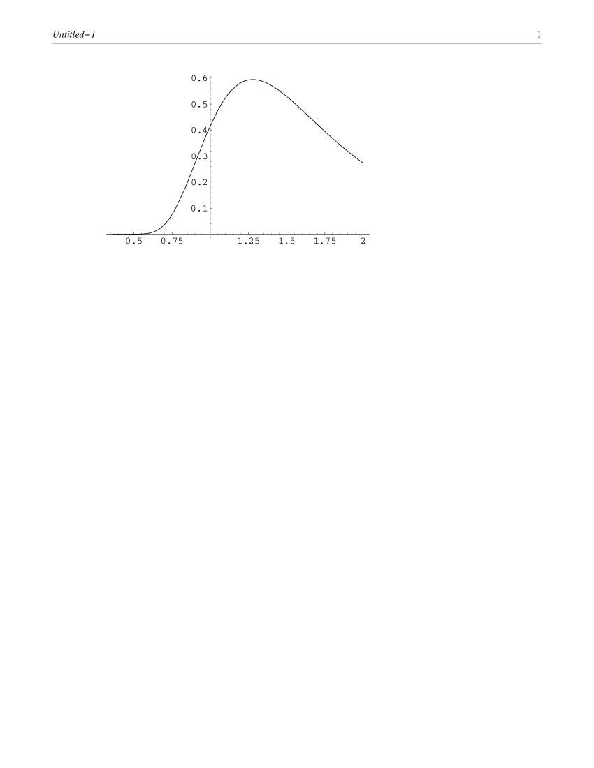
Figure 1: Plot of function $\epsilon(\tilde{\tau}_{0})$ for $\nu=0$.

Figure 2: Plot of function $\tilde{\tau}_{0}(\epsilon)$ for $\nu=0$.

Let us write the exponent $F(\epsilon,\nu)$ of the cross section (8) as

$$F(\epsilon,\nu)=-32\pi^{2}+F^{(1)}(\epsilon,\nu)+F^{(2)}(\epsilon,\nu)+\ldots,$$

where $F^{(1)}(\epsilon,\nu)$ and $F^{(2)}(\epsilon,\nu)$ are given by $\hat{W}$ and $W^{(2)}$, respectively, evaluated at the saddle point solution. Substituting solutions (99) - (101) into Eq. (6) we obtain that

$$F^{(1)}(\epsilon,\nu)=\kappa\epsilon\left[\tilde{\tau}_{0}(\epsilon)+\frac{1}{4\Phi^{\prime}(\tilde{\tau}_{0}(\epsilon))}\right]+{\cal O}(\nu).$$ (104)

For $0\leq\tilde{\tau}_{0}\leq 1.28$ the function $\epsilon(\tilde{\tau}_{0})$ grows monotonically from $\epsilon=0$ to $\epsilon\approx 0.59$ (see Fig. 1). Hence, for the interval $0\leq\epsilon\leq 0.59$ there exists the inverse function $\tilde{\tau}_{0}(\epsilon)$ with the property $\tilde{\tau}_{0}(0)=0$. This is also the interval of energies for which the saddle point solution at $\nu=0$ can be found. The plot in Fig. 2 shows that for $0\leq\epsilon\leq 1.59$ the values of $\tilde{\tau}_{0}(\epsilon)$ in general are not small. Since $\tilde{\tau}$ is the saddle point solution for $\tau m$, this observation suggests that the mass corrections cannot be neglected. For $0<\epsilon<0.1$ we enter the regime when $\tilde{\tau}_{0}<1$ and the expressions for the saddle point solution and Eq. (104) simplify considerably. In particular, $\Phi(\tilde{\tau}_{0})\sim 1/\tilde{\tau}_{0}^{2}$ for $\tilde{\tau}_{0}\ll 1$. In this regime corrections due to non-zero mass can be neglected.

At very small energies, namely when

$$\frac{\ln\ln\frac{1}{\epsilon}}{\ln\frac{1}{\epsilon}}\ll 1,$$ (105)

we enter the regime when analytical expressions for the saddle point solutions can be obtained. The function $\tilde{\tau}_{0}(\tilde{\epsilon})$ is small in this limit. In the leading approximation Eq. (103) takes the form

$$\ln\tilde{\epsilon}+\frac{4}{\tilde{\tau}_{0}^{2}}+5\ln\tilde{\tau}_{0}+\ln\left(\frac{Ce}{2\upsilon}\right)+2C_{E}-1+\ldots=0,$$

where the dots stand for terms vanishing as $\tilde{\epsilon}\rightarrow 0$. It is easy to obtain the asymptotic form of the solution of this equation in for the variable $1/\tilde{\tau}_{0}(\tilde{\epsilon})$. We get

$$\frac{1}{\tilde{\tau}_{0}^{2}(\tilde{\epsilon})}=\frac{1}{4}\ln\frac{1}{\tilde{\epsilon}}+\frac{5}{8}\ln\ln\frac{1}{\tilde{\epsilon}}+\ln\upsilon-4C_{E}-1+\;\;\mbox{decreasing terms}.$$

The first two leading terms of the function $\tilde{\tau}_{0}(\tilde{\epsilon})$ are given by

$$\tilde{\tau}_{0}(\tilde{\epsilon})=\frac{2}{\sqrt{\ln\frac{1}{\tilde{\epsilon}}}}-\frac{5}{2}\frac{\ln\ln\frac{1}{\tilde{\epsilon}}}{\left(\ln\frac{1}{\tilde{\epsilon}}\right)^{3/2}}+\ldots$$ (106)

Then in the leading order in energy solutions (99) - (101) become

$$\tilde{\rho}^{2}=\frac{1}{48\pi^{2}}\frac{\tilde{\epsilon}}{\left(\ln\frac{1}{\tilde{\epsilon}}\right)^{3/2}},\quad\tilde{\gamma}=\left(\frac{\tilde{\nu}}{\tilde{\epsilon}}\right)^{3}\left(\ln\frac{1}{\tilde{\epsilon}}\right)^{3/2},\quad(\tilde{\chi}-\tilde{\tau})=2\frac{\tilde{\nu}}{\tilde{\epsilon}}.$$ (107)

In this regime the function $F^{(1)}(\epsilon,\nu)$ is equal to

$$F^{(1)}(\epsilon,\nu)=2\frac{\kappa\epsilon}{\sqrt{\ln\frac{1}{\epsilon}}}\left[1+{\cal O}\left(\frac{\ln\ln\frac{1}{\epsilon}}{\ln\frac{1}{\epsilon}}\right)\right]+{\cal O}(\nu).$$ (108)

This is result (6) quoted in the Introduction.

The propagator correction $F^{(2)}(\epsilon,\nu)$ in the limit $\nu\rightarrow 0$ is obtained by evaluating contributions (35) - (2) at the saddle point solution (99) - (101). In Sect. 2 we showed in a rather general context that singular terms $\ln(1/\nu)$ appear in the contributions involving initial particles and proved that they cancel each other in the final result. Let us discuss now the exact expression for the propagator correction for the $(-\lambda\phi^{4})$-model in the limit $\nu\rightarrow 0$. The result for the partial contributions is given by Eqs. (A3) - (A8) in the Appendix. We see that singular terms $\ln(1/\tilde{\nu})$ appear only in the functions $F^{(2)}_{(i-i)}(\epsilon,\nu)$ and of $F^{(2)}_{(i-f)}(\epsilon,\nu)$ which involve initial states and which are proportional to $\alpha_{1}$. Hence, according to Eq. (88), the singular terms are due to $s\ln s$- and $s$-terms in the instanton propagator. It is clear now that, if following the method of Ref. [12], reviewed in Sect. 4, one chooses the propagator constraint in such way that these terms are absent in the residue, then the contributions of the initial states are zero in the limit $\nu\rightarrow 0$. Correspondingly, in this case no singular terms appear.

As it follows from these formulas and the saddle point solution (106), in the limit of small energies the corrections $F^{(2)}_{(i-i)}(\epsilon,\nu)$ and of $F^{(2)}_{(i-f)}(\epsilon,\nu)$ behave as

$$\sim\frac{\epsilon^{3}}{\left(\ln\frac{1}{\epsilon}\right)^{3/2}}.$$

The contribution $F^{(2)}_{(f-f)}(\epsilon,\nu)$ of the final states contains a part $\sim\alpha_{1}$ and a part $\sim\alpha_{2}$. The former is due to $s\ln s$- and $s$-terms in the instanton propagator residue, the latter is due to $\ln s$-terms and $s$-independent terms of it (see Eq. (88). In the limit of small energies $F^{(2)}_{(f-f)}(\epsilon,\nu)$ behaves as $\epsilon^{2}$, thus giving the dominant contribution to the propagator correction.

As an illustration let us demonstrate the cancellation of the singular terms explicitly in our model. Summing up corrections (A4) and (A6) we get

$$F^{(2)}_{(i-i)}(\epsilon,\nu)+F^{(2)}_{(i-i)}(\epsilon,\nu)=32\alpha_{1}\upsilon\tilde{\rho}^{6}$$

$$\times\left\{-\frac{\tilde{\gamma}}{2(\tilde{\chi}-\tilde{\tau})^{3}}\left[\frac{2\gamma}{(\tilde{\chi}-\tilde{\tau})^{3}}+\Phi^{\prime}(\tilde{\tau})\right]\cdot\left[\frac{71}{30}+\ln\frac{\tilde{\rho}^{2}}{(\tilde{\chi}-\tilde{\tau})^{2}}\right]\right.$$

$$\left.-\frac{\tilde{\gamma}}{2(\tilde{\chi}-\tilde{\tau})^{3}}\Phi^{\prime}(\tilde{\tau})\ln\frac{\tilde{\rho}^{2}}{\tilde{\tau}^{2}}+\frac{\tilde{\gamma}}{2(\tilde{\chi}-\tilde{\tau})^{3}}\Phi^{\prime}(\tilde{\tau})\left(2\ln 2-\frac{71}{30}\right)+\frac{\tilde{\gamma}}{(\tilde{\chi}-\tilde{\tau})^{3}}{\cal A}_{1}(\tilde{\tau})\right\}.$$

The singular term is $\ln(\tilde{\rho}^{2}/(\tilde{\chi}-\tilde{\tau})^{2})\sim\ln(1/\tilde{\nu})$ in the second line. The coefficient in front of it vanishes exactly due to the saddle point equation (98).

Finally, let us present the result for the complete propagator correction to the exponent of the multiparticle cross section in the limit $\nu\rightarrow 0$. Summing up expressions (A4), (A6) and (A8) for the partial corrections, we obtain

$$F^{(2)}(\epsilon,0) = -\frac{\alpha_{2}}{\upsilon}\tilde{\epsilon}^{2}\frac{4\Phi^{2}(\tilde{\tau})}{\left(\Phi^{\prime}(\tilde{\tau})\right)^{2}}\left[\frac{43}{15}-\ln 2-2C_{E}-4\Phi(\tilde{\tau})-\ln\frac{\tilde{\tau}^{2}}{4}+\frac{{\cal A}_{A}(\tilde{\tau})}{\Phi^{2}(\tilde{\tau})}\right]$$

$$- \frac{8\alpha_{1}}{\upsilon^{2}}\frac{\tilde{\epsilon}^{3}}{\Phi^{\prime}(\tilde{\tau})}\left\{\frac{1}{2}-\ln 2-2\frac{{\cal A}_{1}(\tilde{\tau})}{\Phi^{\prime}(\tilde{\tau})}-\frac{{\cal A}_{3}(\tilde{\tau})}{\left(\Phi^{\prime}(\tilde{\tau})\right)^{2}}\right.$$

$$+ \left.\frac{\Phi^{2}(\tilde{\tau})}{\left(\Phi^{\prime}(\tilde{\tau})\right)^{2}}\left[-\ln 2-\frac{2}{15}-2C_{E}-4\Phi(\tilde{\tau})-2\ln\frac{\tilde{\tau}}{2}\right]\right\}.$$

The expression for the propagator correction simplifies in the regime $\tilde{\tau}_{0}\ll 1$. In this case, using Eqs.(A10), (A11) and (Appendix A) or calculating the limit of small $\tilde{\tau}_{0}$ directly from Eq. (6), one gets

$$F^{(2)}(\epsilon,0) = \frac{4\alpha_{2}}{\upsilon}\tilde{\epsilon}^{2}\left[1+\frac{\tilde{\tau}_{0}^{2}}{4}\left(8\ln\frac{\tilde{\tau}_{0}}{2}+8C_{E}-\frac{43}{15}\right)+{\cal O}(\tilde{\tau}_{0}^{4})\right]$$

$$- \frac{4\alpha_{1}}{\upsilon^{2}}(\tilde{\epsilon}\tilde{\tau}_{0})^{3}\cdot{\cal O}\left(\tilde{\tau}_{0}^{2},\tilde{\tau}_{0}^{2}\ln\tilde{\tau}_{0}\right).$$

The first line is the leading term at small energies:

$$F^{(2)}(\epsilon,0)=\frac{4\alpha_{2}}{\upsilon}\tilde{\epsilon}^{2}=\frac{1}{32\pi^{2}}\kappa^{2}\epsilon^{2}.$$ (111)

As it was discussed above, this is the contribution from the propagator between final-final state. The first correction to expression (111) is given by the $\tilde{\tau}^{2}\ln\tilde{\tau}$ term in Eq. (6). In the regime of very small energies we have

$$\tilde{\tau}_{0}^{2}\ln\tilde{\tau}_{0}\sim\frac{\ln\ln\frac{1}{\epsilon}}{\ln\frac{1}{\epsilon}}.$$

By comparing the propagator correction (111) with the leading order correction (108) we see that the actual expansion parameter at small energies is indeed $\epsilon\sqrt{\ln(1/\epsilon)}$, as it was argued in Ref. [14].

7 Propagator correction in general case

For arbitrary $\epsilon$ and $\nu$ the saddle point equations are obtained by calculating of the derivatives of the general expression $\hat{W}$, Eq. (6), with respect to $\rho^{2}$, $\gamma$, $\chi$ and $\tau$. In this case we found the saddle point solutions $\tilde{\rho}^{2}(\epsilon,\nu)$, $\tilde{\tau}(\epsilon,\nu)$, $\tilde{\chi}(\epsilon,\nu)$, $\tilde{\gamma}(\epsilon,\nu)$ for $(m\rho)^{2}$, $m\tau$, $m\chi$, $\gamma$, respectively, and computed the functions $F^{(1)}(\epsilon,\nu)$, $F^{(2)}(\epsilon,\nu)$ numerically. It turned out that the saddle point solution exists only for the region in the $(\epsilon,\nu)$-plane which is presented in Fig. 3. It lies inside the rectangle $0<\epsilon<\epsilon_{max}=0.59$ and $0<\nu<\nu_{max}=0.25$. For points very close to the axis $\nu=0$ our numerical computations fail. Extrapolating these numerical results to $\nu=0$ we found good agreement with the analytical results for $\nu=0$ obtained in Sect. 6.

Figure 3: Region of values of $\epsilon$ and $\nu$ for which the saddle point solution exists.

We performed the numerical analysis for the whole region, plotted in Fig. 3. For the presentation of the results it is convenient to introduce the function ${\cal F}(\epsilon,\nu)$, related to $F(\epsilon,\nu)$ by

$$F(\epsilon,\nu)=-32\pi^{2}{\cal F}(\epsilon,\nu),$$ (112)

and its leading and next-to-leading approximations:

$${\cal F}_{1}(\epsilon,\nu)=1-\frac{F^{(1)}(\epsilon,\nu)}{32\pi^{2}},\;\;\mbox{and}\;\;{\cal F}_{2}(\epsilon,\nu)=1-\frac{F^{(1)}(\epsilon,\nu)+F^{(2)}(\epsilon,\nu)}{32\pi^{2}}.$$

All these functions are normalized by the conditions ${\cal F}(0,\nu)={\cal F}_{1}(0,\nu)={\cal F}_{2}(0,\nu)=1$.

Before presenting our results we would like to mention that the complete function $F(\epsilon,\nu)$ in the range $0.4<\epsilon<3.5$ and $0.25<\nu<1$ was computed in Ref. [9]. The computation was performed by solving a certain classical boundary value problem on the lattice. With the size of the lattice used in the numerical calculation in Ref. [9], the authors did not obtain data for smaller $\epsilon$ and $\nu$ except for the line of points corresponding to the periodic instanton solutions [26]. This line is directed from the zero energy instanton ($\epsilon=\nu=0$) to the sphaleron ($\epsilon=\nu=1$).

The left upper bound of the region in Fig. 3 is precisely the line $\nu=\nu_{p}(\epsilon)$ of values of $\epsilon$ and $\nu$ of periodic instantons. For them $\tilde{\tau}(\epsilon,\nu)=\tilde{\chi}(\epsilon,\nu)/2$. The leading order and the next-to-leading order approximations for ${\cal F}(\epsilon,\nu)$ at the line $(\epsilon,\nu_{p}(\epsilon))$ are shown in Fig. 4. One can see that in the whole range of calculation these curves are close to each other. They can be compared with the complete function ${\cal F}(\epsilon,\nu_{p}(\epsilon))$ for the line of periodic instantons, computed numerically in Ref. [9] and also plotted in Fig. 4. The comparison shows that our perturbative results do not differ significantly from the exact ones for $\epsilon<0.25$ and $\nu<0.2$. These values can be regarded as a rough estimate of the range of validity of the perturbative calculations up to the next-to-leading order.

Figure 4: Plots of ${\cal F}_{1}(\epsilon,\nu_{p}(\epsilon))$ (the lower curve) and ${\cal F}_{2}(\epsilon,\nu_{p}(\epsilon))$ as functions of $\epsilon$ for the periodic instanton. For comparison the complete function ${\cal F}(\epsilon,\nu_{p}(\epsilon))$ (the longer curve), calculated in Ref. [9], is also plotted.

Lines of constant ${\cal F}_{2}(\epsilon,\nu)$ are plotted in Fig. 5. Within the range of $(\epsilon,\nu)$ in Fig. 3 the minimal value of ${\cal F}(\epsilon,\nu)$ is a bit below ${\cal F}=0.77$. This gives still a considerable suppression of the multiparticle cross section of instanton induced processes.

Figure 5: Lines of constant ${\cal F}_{2}(\epsilon,\nu)$ in the $(\epsilon,\nu)$-plane. Numbers near the lines indicate the value of ${\cal F}_{2}$, “p” labels the line of periodic instanton solutions.

As it was explained above, our main interest is to study the cross section for shadow processes with a few initial particles. According to conjecture (10) the points, where the lines of constant ${\cal F}_{2}$ cross the $\nu=0$ axis, are of particular interest. Extrapolating our numerical results to $\nu=0$, one obtains, for example, ${\cal F}_{2}(\epsilon,0)=0.95$ at $\epsilon=0.180$, ${\cal F}_{2}(\epsilon,0)=0.85$ at $\epsilon=0.492$. These values, of course, can be obtained by using the exact formulas for $\nu=0$ from Sect. 6. We would like to mention that in the region of $(\epsilon,\nu)$ which we studied the next-to-leading approximation ${\cal F}_{2}(\epsilon,\nu)$ is quite small comparing to the leading order ${\cal F}_{1}(\epsilon,\nu)$. The difference between these functions does not exceed $10^{-2}$. The curves in Fig. 5 end at the line formed by saddle points of the periodic instanton solutions.

In Sect. 5 we mentioned that various expressions for the functions $s_{\#}({\bf k},{\bf q})$ can be used in the definition of the residue of the instanton propagator, Eq. (83). Examples of such functions are given by Eqs. (24), (25) and (84), (85). We performed the calculation of the leading and next-to-leading order approximations for these particular choices of functions and for a wide range of values of $\epsilon$ and $\nu$. We found that the difference is very tiny. Thus,

$${\cal F}_{2}(0.2,\nu_{p}(0.2))|_{\tilde{s}_{aa},\tilde{s}_{ab}}-{\cal F}_{2}(0.2,\nu_{p}(0.2))|_{s_{aa},s_{ab}}\approx 5\cdot 10^{-4}.$$

8 Accuracy of the approximation

As it was explained in Sect. 3, in principle the constrained instanton configuration and the action of this configuration depend on the constraints imposed. In Eq. (61) we calculated only the leading, constraint independent part of the action. This is main restriction to the accuracy which can be achieved in our calculations. Corrections due to the form of the constraint after evaluation at the saddle point solution are of the order $\tilde{\rho}^{4}$, $\tilde{\rho}^{2}\ln\tilde{\rho}$ or $\tilde{\rho}^{2}\ln^{2}\tilde{\rho}$ (see Eq. (61)). It turns out that within this accuracy main terms of the leading and propagator contributions to $F(\epsilon,\nu)$ can be calculated. For this one has to follow a certain scheme of approximations, which we discuss in the present section.

Let us first obtain some simple estimates of the leading and next-to-leading corrections at $\nu\rightarrow 0$. For the case when $m\tau\ll 1$ the dominating term of the leading correction is given by $\rho^{2}J_{0}(\gamma,\tau,\chi)\sim\rho^{2}/\tau^{2}$. From the analysis of the next-to-leading one can show that the main term is $F_{(f-f)}^{(2)}$, which is due to the instanton propagators between the final states. For small $m\tau$ the dominant contribution to the integrals in Eq. (2) are given by the soft momenta $|{\bf k}|\sim|{\bf q}|\sim 1/\tau$. For such momenta the $\ln(\rho^{2}s)$-term in the expression (88) for the residue of the instanton propagator plays the main role. Putting all the factors together one can see that $F^{(2)}\sim F^{(2)}_{(f-f)}\sim(\rho/\tau)^{4}\ln(\rho/\tau)^{2}$. To summarize, in this regime

$$F^{(1)}(\epsilon,\nu)\sim\frac{\rho^{2}}{\tau^{2}},\;\;\;F^{(2)}(\epsilon,\nu)\sim\frac{\rho^{4}}{\tau^{4}}\ln\frac{\rho^{2}}{\tau^{2}}.$$ (113)

These estimates are in agreement with results (104), (6) and (A7). To see this one should use formula (99) for $\tilde{\rho}^{2}$ and take into account that for $\tilde{\tau}\ll 1$

$$\tilde{\epsilon}\tilde{\tau}\sim\tilde{\rho}^{2}\tilde{\tau}\Phi^{\prime}(\tilde{\tau})\sim\frac{\tilde{\rho}^{2}}{\tilde{\tau}^{2}}$$

in Eq. (104), and

$$\tilde{\rho}^{4}\Phi^{2}(\tilde{\tau})\ln\frac{\tilde{\rho}^{2}}{\tilde{\tau}^{2}}\sim\frac{\tilde{\rho}^{4}}{\tilde{\tau}^{4}}\ln\frac{\tilde{\rho}^{2}}{\tilde{\tau}^{2}}$$

in Eq. (A7). For very small energies from solutions (106), (107) one gets

$$\frac{\tilde{\rho}^{2}}{\tilde{\tau}^{2}}\sim\frac{\epsilon}{\sqrt{\ln\frac{1}{\epsilon}}},\;\;\;\frac{\tilde{\rho}^{4}}{\tilde{\tau}^{4}}\ln\frac{\tilde{\rho}^{2}}{\tilde{\tau}^{2}}\sim\epsilon^{2}$$ (114)

in accordance with results (108) and (111).

To have numerical estimates of the range of values of these characteristic terms we studied the saddle point solution $\tilde{\rho}^{2}(\epsilon,\nu)$ and the ratio $\tilde{\rho}^{2}(\epsilon,\nu)/\tilde{\tau}^{2}(\epsilon,\nu)$ numerically for a wide range of $\epsilon$ and $\nu$. In Fig. 6 and Fig. 7 we present the plots of these functions for the most interesting case $\nu=0$.

Figure 6: Plot of the function $\tilde{\rho}^{2}(\epsilon,0)$.

Figure 7: Plot of the function $\tilde{\rho}^{2}(\epsilon,0)/\tilde{\tau}^{2}(\epsilon,0)$.

For the procedure of calculation to be consistent one has to check, first of all, that $\tilde{\rho}^{4}$, $\tilde{\rho}^{4}\ln\tilde{\rho}$ and $\tilde{\rho}^{4}\ln^{2}\tilde{\rho}$ are smaller than the propagator correction $F^{(2)}(\epsilon,\nu)$. We checked numerically that this is indeed the case for a wide range of $\epsilon$ and $\nu$. In general, since, as it was mentioned in Sect. 7, $|{\cal F}_{1}-{\cal F}_{2}|\leq 10^{-3}$, the propagator correction $F^{(2)}\leq 0.3$, whereas $\tilde{\rho}^{4}\leq 10^{-4}$. Thus, at the point $\epsilon=0.2$, $\nu_{p}(0.2)=0.17$ on the line of periodic instantons $F^{(2)}(0.2,0.17)=0.28$, whereas $\tilde{\rho}^{2}(0.2,0.17)\approx 0.02$. Another example: for $\nu=0$ $F^{(2)}(0.33,0)\approx 0.3$, whereas $\tilde{\rho}^{2}(0.33,0)\approx 0.01$. From Fig. 6) and Fig. 7 one can see that the corrections $\tilde{\rho}^{4}$, $\tilde{\rho}^{4}\ln\tilde{\rho}$ and $\tilde{\rho}^{4}\ln^{2}\tilde{\rho}$ are smaller than $F^{(2)}(\epsilon,\nu)$ for the regime when $\tilde{\tau}<1$ (see Eq. (113). This conclusion is also confirmed for $\nu=0$ in the limit of very small energies. Using formulas (106), (107) one can see that

$$\tilde{\rho}^{4}\sim\frac{\epsilon^{2}}{\left(\ln\frac{1}{\epsilon}\right)^{3}},\;\;\;\tilde{\rho}^{4}\ln\tilde{\rho}\sim\frac{\epsilon^{2}}{\left(\ln\frac{1}{\epsilon}\right)^{2}},\;\;\;\tilde{\rho}^{4}\ln^{2}\tilde{\rho}\sim\frac{\epsilon^{2}}{\ln\frac{1}{\epsilon}}.$$

Recall that the propagator correction $F^{(2)}(\epsilon,0)\sim\epsilon^{2}$ in this regime (see Eqs. (111) and (114)). To give an illustration we presented the plot of the function $\tilde{\rho}(\epsilon,0)$ in Fig. 6.

It turns out that with the accuracy set above it is enough to use the residue of the instanton solution $I(\rho)$ and the double on-mass-shell residue of the instanton propagator $P({\bf k},{\bf q})$ of the massless theory. Let us justify this point.

Let $\phi_{c.i.}(x;\rho)$ be the constrained instanton solution of the size $\rho$ in the massive theory. From general arguments one can see that its Fourier transform can be written as

$$\tilde{\phi}_{c.i.}(k;0,\rho)=\rho\frac{g(k^{2}\rho^{2},m^{2}\rho^{2})}{k^{2}+m^{2}}.$$

Expanding the function $g(k^{2}\rho^{2},m^{2}\rho^{2})$ in powers of $m^{2}$ we write

$$g(k^{2}\rho^{2},m^{2}\rho^{2})=g_{0}(k^{2}\rho^{2})+(\rho m)^{2}g_{2}(k^{2}\rho^{2})+\ldots$$

Logarithmic terms of the form $(\rho m)^{2}\ln(\rho m)$ may also appear, however we will not write them explicitly assuming that they are roughly of the order $(\rho m)^{2}$. The residue $I_{c.i.}(\rho)=(k^{2}+m^{2})\tilde{\phi}_{c.i.}(k;\rho)|_{k_{0}=iw_{{\bf k}}}$ is equal to

$$I_{c.i.}(\rho)=\rho g_{0}(0)+\rho(\rho m)^{2}\left(g_{2}(0)-g_{0}^{\prime}(0)\right)+\ldots$$

Since the constrained instanton solution reproduces the instanton solution $\phi_{inst}(x;0,\rho)$, Eq. (60), of the massless theory in the limit $m\rightarrow 0$, the Fourier transform of $\phi_{inst}$ and its residue can be written as

$$\tilde{\phi}_{inst}(k;0,\rho)=\rho\frac{g_{0}(k^{2}\rho^{2})}{k^{2}},\;\;\;I(\rho)=\rho g_{0}(0).$$

These formulas are in accordance with exact expressions (78) and (79).

Typical terms of the leading order correction are of the form

$$\int\frac{d{\bf k}}{w_{{\bf k}}}I_{c.i.}(\rho)K(w_{{\bf k}}\tau,w_{{\bf k}}\chi)I_{c.i.}(\rho),$$ (115)

where

$$K(w_{{\bf k}}\tau,w_{{\bf k}}\chi)=\frac{e^{-w_{{\bf k}}\tau}}{1-\gamma e^{-w_{{\bf k}}\chi}}$$ (116)

(see Eq. (6)). By a simple analysis one can show that

$$\int\frac{d{\bf k}}{w_{{\bf k}}}I_{c.i.}(\rho)K(w_{{\bf k}}\tau,w_{{\bf k}}\chi)I_{c.i.}(\rho)$$

$$=\int\frac{d{\bf k}}{w_{{\bf k}}}I_{inst}(\rho)K(w_{{\bf k}}\tau,w_{{\bf k}}\chi)I_{inst}(\rho)+{\cal O}\left(m\rho^{2}\frac{\rho^{2}}{\tau^{2}}\right).$$

We checked that the ratio $\tilde{\rho}^{4}/\tilde{\tau}^{2}$ is small comparing to $F^{(2)}(\epsilon,\nu)$ for a wide range of $\epsilon$ and $\nu$. This can also be seen from the plots in Fig. 6) and Fig. 7. In the regime of very small energies from Eqs. (106), (107) one gets

$$\tilde{\rho}^{2}\frac{\tilde{\rho}^{2}}{\tilde{\tau}^{2}}\sim\frac{\epsilon^{2}}{\left(\ln\frac{1}{\epsilon}\right)^{2}},$$

whereas $F^{(2)}(\epsilon,0)\sim\epsilon^{2}$.

However, if the expression $w_{{\bf k}}=|{\bf k}|$ of the massless theory is used in (115), then by simple estimates one can see that

$$\int\frac{d{\bf k}}{w_{{\bf k}}}I(\rho)K(w_{{\bf k}}\tau,w_{{\bf k}}\chi)I(\rho)\sim\int\frac{d{\bf k}}{|{\bf k}|}I(\rho)K(|{\bf k}|\tau,|{\bf k}|\chi)I(\rho)+\frac{\rho^{2}}{\tau^{2}}\cdot{\cal O}(m^{2}\tau^{2}).$$ (117)

Since the saddle point solution $\tilde{\tau}(\epsilon,\nu)\geq 1$ for a range of values of $\epsilon$ and $\nu$ (see, for example, Fig. 2), relation (117) warns that the corrections due to non-zero mass cannot be discarded. In particular, for the regime of very small energies and $\nu=0$ the term $(\tilde{\rho}^{2}/\tilde{\tau}^{2})\tilde{\tau}^{2}\sim\epsilon/\ln(1/\epsilon)$ and obviously exceeds the propagator correction $F^{(2)}\sim\epsilon^{2}$. The conclusion is the following: in order to be within the accuracy set above one has to use the expression $w_{{\bf k}}=\sqrt{{\bf k}^{2}+m^{2}}$ for the energy, though it is enough to use the residue $I(\rho)$ of the instanton solution of the massless theory.

For the residue of the instanton propagator and the propagator correction a similar analysis can be carried out. A general expression for the Fourier transform of the instanton propagator in the massive theory is of the form

$$G_{\psi}(k,q)=\rho^{2}\frac{h(k^{2}\rho^{2},q^{2}\rho^{2},s\rho^{2},m^{2}\rho^{2})}{(k^{2}+m^{2})(q^{2}+m^{2})},$$

where $s=(k+q)^{2}$. Expanding the function in the numerator in powers of $m^{2}\rho^{2}$,

$$h(k^{2}\rho^{2},q^{2}\rho^{2},s\rho^{2},m^{2}\rho^{2})=h_{0}(k^{2}\rho^{2},q^{2}\rho^{2},s\rho^{2})+(\rho m)^{2}h_{2}(k^{2}\rho^{2},q^{2}\rho^{2},s\rho^{2})+\ldots$$

(logarithmic terms, like $\rho^{2}m^{2}\ln(\rho^{2}m^{2})$, may also appear), we obtain that the double on-mass-shell residue of the propagator can be written as

$$P^{(m)}(s_{\#}\rho^{2}) = \rho^{2}h_{0}(0,0,s_{\#}\rho^{2})+\rho^{2}(\rho m)^{2}\left[h_{2}(0,0,s_{\#}\rho^{2})\right.$$

$$- \left.h_{01}^{\prime}(0,0,s_{\#}\rho^{2})-h_{02}^{\prime}(0,0,s_{\#}\rho^{2})\right],$$

where $\#=aa,ab,bb$, $s_{\#}$ is given by Eqs. (24), (25) and the upper index $(m)$ refers to the non-zero mass case. It is easy to see that the residue of the instanton propagator in the massless theory is then given by

$$P(s\rho^{2})=\rho^{2}h_{0}(0,0,s\rho^{2}).$$

A typical term in the propagator correction is

$$\rho^{2}\int\frac{d{\bf k}}{w_{{\bf k}}}\frac{d{\bf q}}{w_{{\bf q}}}I_{c.i.}K(w_{{\bf k}}\tau_{1},w_{{\bf k}}\chi)P^{(m)}(\rho^{2}s_{\#}({\bf k},{\bf q}))K(w_{{\bf q}}\tau_{2},w_{{\bf q}}\chi)I_{c.i.},$$

where $K(w_{{\bf k}}\tau_{1},w_{{\bf q}}\chi)$ is defined by Eq. (116). By a simple analysis one gets

$$\rho^{2}\int\frac{d{\bf k}}{w_{{\bf k}}}\frac{d{\bf q}}{w_{{\bf q}}}I_{c.i.}K(w_{{\bf k}}\tau_{1},w_{{\bf k}}\chi)P^{(m)}(\rho^{2}s_{\#}({\bf k},{\bf q}))K(w_{{\bf q}}\tau_{2},w_{{\bf q}}\chi)I_{c.i.}$$

$$=\rho^{2}\int\frac{d{\bf k}}{w_{{\bf k}}}\frac{d{\bf q}}{w_{{\bf q}}}IK(w_{{\bf k}}\tau_{1},w_{{\bf k}}\chi)P(\rho^{2}s_{\#}({\bf k},{\bf q}))K(w_{{\bf q}}\tau_{2},w_{{\bf q}}\chi)I$$

$$+{\cal O}\left(\frac{\rho^{4}}{\tau^{4}}(\rho m)^{2},(\rho m)^{6}\right).$$

Again, from our numerical results we see that the corrections are small comparing to the propagator correction $F^{(2)}(\epsilon,\nu)$, calculated with $I$ and $P(\rho^{2}s)$, and can be neglected without loss of accuracy. Similar to estimate (117), if instead of $w_{{\bf k}}=\sqrt{{\bf k}^{2}+m^{2}}$ and $s_{\#}({\bf k},{\bf q})$ the expressions $|{\bf k}|$ and $s_{\#}^{(0)}({\bf k},{\bf q})$, Eq. (82), respectively, are used, then one can easily show that

$$\rho^{2}\int\frac{d{\bf k}}{w_{{\bf k}}}\frac{d{\bf q}}{w_{{\bf q}}}IK(w_{{\bf k}}\tau_{1},w_{{\bf k}}\chi)P(\rho^{2}s_{\#}({\bf k},{\bf q}))K(w_{{\bf q}}\tau_{2},w_{{\bf q}}\chi)I$$

$$=\rho^{2}\int\frac{d{\bf k}}{|{\bf k}|}\frac{d{\bf q}}{|{\bf q}|}IK(|{\bf k}|\tau_{1},|{\bf k}|\chi)P(\rho^{2}s_{\#}^{(0)}({\bf k},{\bf q}))K(|{\bf q}|\tau_{2},|{\bf q}|\chi)I$$

$$+\left(\frac{\rho}{\tau}\right)^{4}{\cal O}\left((m\tau)^{2},(m\rho)^{2}\ln\frac{\rho^{2}}{\tau^{2}},(m\rho)^{2}\right),$$ (118)

where we assumed that $\tau\sim\tau_{1}\sim\tau_{2}$. Since for a certain range of $\epsilon$ and $\nu$ the saddle point value $\tilde{\tau}\sim 1$, Eq. (118) gives an indication that the mass corrections can be comparable to the propagator correction $F^{(2)}\sim(\tilde{\rho}/\tilde{\tau})^{4}\ln(\tilde{\rho}^{2}/\tilde{\tau}^{2})$ and should be taken into account.

Now we can formulate a procedure of calculation of the leading and next-to-leading order corrections to the function $F(\epsilon,\nu)$ as follows: in expressions for $\hat{W}$ and $W^{(2)}$

1)

the residue of the instanton solution $I(\rho)$, given by Eq. (79), and the residue of the instanton propagator $P(\rho^{2}s)$, given by Eq. (87), of the massless theory are substituted;

2)

the energy $w_{{\bf k}}$ and the $s$-variables $s_{aa}$, $s_{ab}$ and $s_{bb}$, given by Eqs. (24), (25) (or by by Eqs. (84), (85)) of the massive theory are used.

We have shown that this procedure is consistent and gives results which are within the accuracy, set by Eq. (61), provided $\tilde{\rho}^{2}(\epsilon,\nu)$ and $\tilde{\rho}^{2}(\epsilon,\nu)/\tilde{\tau}^{2}(\epsilon,\nu)$ are small in the range of our calculations. From the results of our numerical computations in Sect. 7 we checked that this condition holds.

9 Discussion and conclusions

In the present paper we have analyzed the multiparticle cross section of the shadow processes induced by instanton transitions in the simple scalar model with the action given by Eq. (59). We calculated the exact analytical expression for the on-shell residue of the propagator of quantum fluctuations in the instanton background. Using this result we calculated the propagator correction (i.e. the next-to-leading order correction) to the suppression factor $F/\lambda$ of the multiparticle cross section.

The leading and next-to-leading (propagator) corrections to the function $F(\epsilon,\nu)$ were calculated semiclassically, by evaluation of the leading and next-to-leading terms in Eq. (12), respectively, at the saddle point.

Within the accuracy of the approximation, considered in this article, the saddle point equations are derived from the leading terms, Eqs. (13), (14), in the ”effective action”. It turned out, that for such equations the saddle point solutions for the dimensionless parameters $(m\rho)^{2}$, $(m\tau)^{2}$, $(m\chi)^{2}$ and $\gamma$ in the integral (12) exist only for a certain region of $\epsilon=E/E_{sph}$ and $\nu=N/N_{sph}$, shown in Fig. 3.

For general $\epsilon$ and $\nu$ from this region we computed the leading and propagator corrections to the function $F(\epsilon,\nu)$ numerically. For $\nu=0$ we derived the analytical expressions for $F^{(1)}(\epsilon,0)$ and $F^{(2)}(\epsilon,0)$, Eqs. (104), (A3) - (A8), in terms of the saddle point solution $\tilde{\tau}_{0}(\epsilon)$ of Eq. (103). For the regime of very small energies, namely when relation (105) holds, and $\nu=0$ we obtained explicit expressions for the saddle point solutions and the leading and propagator corrections to $F(\epsilon,0)$. Recall that according to conjecture (10) this is the function $F(\epsilon,0)$ which characterizes the cross section of the instanton induced processes with a few initial particles.

The corrections $F^{(1)}(\epsilon,\nu)$ and $F^{(2)}(\epsilon,\nu)$ approach zero value when $\epsilon\rightarrow 0$. However, apparently there is no clear expansion parameter. At $\nu=0$ one can see that at energies for which $\tilde{\tau}(\epsilon)\ll 1$

$$F^{(1)}(\epsilon,0) = 2\upsilon\left(\frac{\tilde{\rho}^{2}}{\tilde{\tau}^{2}}\right)+\ldots,$$ (119)

$$F^{(2)}(\epsilon,0) = F^{(2)}_{(f-f)}(\epsilon,0)+\ldots=-4\alpha_{2}\upsilon\left(\frac{\tilde{\rho}^{4}}{\tilde{\tau}^{4}}\right)\ln\frac{\tilde{\rho}^{2}}{\tilde{\tau}^{2}}+\ldots.$$

Hence, the combination $(\tilde{\rho}^{2}/\tilde{\tau}^{2})\ln(\tilde{\rho}^{2}/\tilde{\tau}^{2})$ can play the role of the small expansion parameter. For very small energies from Eqs. (106), (107) we obtain that

$$\frac{\tilde{\rho}^{2}(\epsilon,0)}{\tilde{\tau}_{0}^{2}(\epsilon)} = \frac{1}{\upsilon}\frac{\tilde{\epsilon}}{\sqrt{\ln\frac{1}{\tilde{\epsilon}}}}\left[1+{\cal O}\left(\frac{\ln\ln(1/\tilde{\epsilon})}{\ln(1/\tilde{\epsilon})}\right)\right],$$

$$\frac{\tilde{\rho}^{4}(\epsilon,0)}{\tilde{\tau}_{0}^{4}(\epsilon)}\ln\frac{\tilde{\rho}^{2}(\epsilon,0)}{\tilde{\tau}_{0}^{2}(\epsilon)} = -\frac{\tilde{\epsilon}^{2}}{\upsilon^{2}}\left[1+{\cal O}\left(\frac{\ln\ln(1/\tilde{\epsilon})}{\ln(1/\tilde{\epsilon})}\right)\right].$$

We see that in this regime the expansion parameter is $\epsilon\sqrt{\ln(1/\epsilon)}$. With these relations, of course, results (108) and (111) are easily recovered from (119) (recall that $\upsilon=192\pi^{2}$ and $\alpha_{2}=3/2$).

The range of validity of the next-to-leading order of approximation of the function $F(\epsilon,\nu)$ was estimated by comparing our results with numerical computations of the function $F(\epsilon,\nu)$ in Ref. [9] for values of $\epsilon$ and $\nu$ for which the latter can be translated to the case of shadow processes. Such translation and the subsequent comparison of the results was done for the periodic instantons. The comparison shows that our perturbative results do not differ significantly from the exact ones for $\epsilon\leq 0.25$ or, equivalently, for $\nu\leq\nu_{p}(0.25)\approx 0.2$. Thus, the intesection of the region $\epsilon\leq 0.25$, $\nu\leq 0.2$ with the region for which the saddle point solutions exist (Fig. 3) can be regarded as a rough estimate of the range of validity of the next-to-leading approximation.

We would like to mention that, actually, in Ref. [9] the function ${\cal F}(\epsilon,\nu)$ (see Eq. (112)) was calculated for points $(\epsilon,\nu)$ such that $0.5<\epsilon<3$, $0.2<\nu<1$ and $0\leq{\cal F}(\epsilon,\nu)\leq 0.6$. For the range $0\leq\epsilon<0.25$ and $0\leq\nu<0.2$ and away from the line of periodic instantons methods of Ref. [9] do not allow to obtain the value of ${\cal F}$. Therefore, at the moment our perturbative calculations are the only ones which give quantitative behaviour of the supression factor in this range.

We should stress that our result for the propagator correction is only the leading term of the expansion in powers of $(m\rho)^{2}$ and $\rho^{2}/\tau^{2}$. This level of accuracy is determined by the fact that in formula (61) for the action of the constrained instanton terms ${\cal O}(m^{4}\rho^{4})$ were not taken into account. In Sect. 8 we formulated the procedure of calculation of the constraint independent terms of the leading and next-to-leading corrections. The procedure essentially relies on the condition that the saddle point values for $\tilde{\rho}^{2}$ and $\tilde{\rho}^{2}/\tilde{\tau}^{2}$ are small in the range of $(\epsilon,\nu)$ under consideration. We checked that for the numerical saddle point solutions found the condition holds true. This conclusion is also verified analytically for the regime of very small energies, namely when relation (105) is valid. This shows the consistency of the procedure of calculation. From this discussion it is clear that before calculating next-next-to-leading corrections to the function $F(\epsilon,\nu)$ one should compute terms ${\cal O}(\tilde{\rho}^{4})$ in the leading and propagator corrections.

We also proved the cancellation of terms singular in the limit $\nu\rightarrow 0$ in the propagator correction $F^{(2)}(\epsilon,\nu)$ in a rather general context. The proof is essentially based on the general structure of the $W^{(1)}$ and $W^{(2)}$ terms, the saddle point equations and the factorization property of the asymptotics of the propagator residue, following from a general formula of Ref. [18]. As we have explained, the problem of singularities in $\nu$ is closely related to the problem of quasiclassical evaluation of contributions of initial states and initial-final states. In Sect. 4 we discussed this issue within the approach proposed by Mueller in Ref. [12]. Namely, we calculated three leading terms of the asymptotics of the instanton propagator at large $s$ and showed that with the appropriate choice of the propagator constraint the $s\ln s$- and $s$-terms cancell out. According to Ref. [12], with such propagator the problem of semiclassical calculation of contributions due to initial states and initial-final states can be tackled properly.

We expect that our results may provide some insight to the understanding of the structure of the suppression factor of the cross section of instanton induced processes in more realistic models, like QCD and the electroweak theory. They may also help to describe some features of the behaviour of such cross sections for of energies $E\ll E_{sph}$, which are of interest for some planned high energy experiments [10].

Appendix A

Evaluating Eq. (49) at the saddle point solution (99) - (101) with the residue of the instanton propagator given by expression (88) we obtain the propagator correction to the function $F(\epsilon,\nu)$ at $\nu\rightarrow 0$ by straightforward calculation. Before presenting the result let us introduce some definitions and explain the origin of some terms.

First we write the $s$-variables, defined by Eqs. (24), (25), as

$$s_{\#}({\bf k},{\bf q})=2kql_{\#}[a_{\#}(k,q)-\cos\theta],$$

where $\#=aa,ab,bb$, $k$ and $q$ stand for $|{\bf k}|$ and $|{\bf q}|$, respectively, $l_{aa}=l_{bb}=-1$, $l_{ab}=1$, and $\theta$ is the angle between ${\bf k}$ and ${\bf q}$. While calculating the function ${\cal S}_{\#}(k,q)$, given by Eq. (52), one encounters the integrals

$$M_{\#,1}(k,q) = \int_{0}^{\pi}\sin\theta d\theta\ln(a_{\#}(k,q)-\cos\theta)=a_{\#}\ln\frac{a_{\#}+1}{a_{\#}-1}+\ln(a_{\#}^{2}-1)-2,$$

$$M_{\#,2}(k,q) = \int_{0}^{\pi}\sin\theta d\theta(a_{\#}(k,q)-\cos\theta)\ln(a_{\#}(k,q)-\cos\theta)$$ (A1)

$$= \frac{a_{\#}^{2}+1}{2}\ln\frac{a_{\#}+1}{a_{\#}-1}+a_{\#}\ln(a_{\#}^{2}-1)-a_{\#}.$$

The logarithmic terms in the integrands above are due to the logarithmic terms in the function $P(\rho^{2}s)$ (see Eq. (88)). To get contributions to the propagator correction the functions $M_{\#,1}(k,q)$ and $M_{\#,2}(k,q)$ are to be integrated over $k$ and $q$ (see Eq. (51)). Hence, we define

$$N_{\#,i}(\tau_{1},\tau_{2})=\int_{0}^{\infty}\frac{k^{2}dk}{w_{k}}\frac{q^{2}dq}{w_{q}}e^{-w_{k}\tau_{1}}e^{-w_{k}\tau_{2}}(kq)^{i-1}M_{\#,i}(k,q),$$

where $i=1,2$. In particular, we will need the function $N_{ab,2}$ in the case when one of its arguments goes to zero. We define

$$\eta(\tau)=\frac{\tau_{1}^{2}}{2}\left.N_{ab,2}(\tau,\tau_{1})\right|_{\tau_{1}\rightarrow 0}.$$

It can be shown that

$$\eta(\tau)=\int_{0}^{\infty}\frac{k^{3}dk}{w_{k}}e^{-w_{k}\tau}M_{ab,2}(k,\infty),$$

where $M_{ab,2}(k,\infty)$ is calculated from (A1):

$$M_{ab,2}(k,\infty)=\frac{(w_{k}+k)^{2}}{2k^{2}}\ln\frac{w_{k}+k}{m}-\frac{(w_{k}-k)^{2}}{2k^{2}}\ln\frac{w_{k}-k}{m}-\frac{w_{k}}{k}\left(1+2\ln\frac{k}{m}\right).$$ (A2)

The logarithmic terms in the propagator residue $P(\rho^{2}s)$ also give rise to the intrgrals of the form

$$\int_{0}^{\infty}\frac{dk}{w_{k}}\left(\frac{k}{m}\right)^{n}e^{-w_{k}\tau}\ln\frac{k}{m}.$$

They can be written as

$$\frac{d}{d\beta}\left.\int_{0}^{\infty}\frac{dk}{w_{k}}\left(\frac{k}{m}\right)^{\beta}e^{-w_{k}\tau}\right|_{\beta=n}=\frac{d}{d\beta}\left[\frac{1}{\sqrt{\pi}}\left(\frac{2}{m\tau}\right)^{\beta/2}\Gamma\left(\frac{\beta+1}{2}\right)K_{\beta/2}(m\tau)\right]_{\beta=n}.$$

Let us introduce the function

$$\Psi(m\tau)=\frac{1}{m\tau}\frac{d}{d\beta}K_{\beta}(m\tau)|_{\beta=1}+\Phi(m\tau)\left[C_{E}+\ln\frac{m\tau}{2}\right],$$

where $\Phi(m\tau)$ is given by Eq. (93). Finally, we define the functions

$${\cal A}_{1}(m\tau) = -\frac{1}{2}\Psi^{\prime}(m\tau)+\frac{1}{m\tau}\Phi(m\tau)+\frac{1}{2}\eta(\tau),$$

$${\cal A}_{2}(m\tau) = \Phi(m\tau)\Psi(m\tau)+\frac{1}{2}N_{bb,1}(\tau,\tau),$$

$${\cal A}_{3}(m\tau) = \Phi^{\prime}(m\tau)\Psi^{\prime}(m\tau)-\frac{2}{m\tau}\Phi(m\tau)\Phi^{\prime}(m\tau)-\Phi(m\tau)\Psi(m\tau)+\frac{1}{2}N_{bb,2}(\tau,\tau).$$

The partial contributions to the function $F(\epsilon,\nu)$ in the limit $\nu\rightarrow 0$ are equal to

$$F^{(2)}_{(i-i)}(\epsilon,\nu)=-32\alpha_{1}\upsilon\tilde{\rho}^{6}\frac{\tilde{\gamma}^{2}}{(\tilde{\chi}-\tilde{\tau})^{6}}\left[\frac{71}{30}+\ln\frac{\tilde{\rho}^{2}}{(\tilde{\chi}-\tilde{\tau})^{2}}\right]$$ (A3)

$$=\frac{8\alpha_{1}}{\upsilon^{2}}\frac{\tilde{\epsilon}^{3}}{\Phi^{\prime}(\tilde{\tau})}\left[2\ln\frac{1}{\tilde{\nu}}-12\Phi(\tilde{\tau})+2\ln\left(-\upsilon\Phi^{\prime}(\tilde{\tau})\right)-6C_{E}+4\ln 2-\frac{109}{30}\right],$$ (A4)

$$F^{(2)}_{(i-f)}(\epsilon,\nu)=\frac{32\alpha_{1}\upsilon\tilde{\rho}^{6}\tilde{\gamma}}{(\tilde{\chi}-\tilde{\tau})^{3}}\left[-\Phi^{\prime}(\tilde{\tau})\left(\ln\frac{\tilde{\rho}^{2}}{\tilde{\tau}(\tilde{\chi}-\tilde{\tau})}+\frac{71}{30}-\ln 2\right)+{\cal A}_{1}(\tilde{\tau})\right]$$ (A5)

$$=-\frac{16\alpha_{1}}{\upsilon^{2}}\frac{\tilde{\epsilon}^{3}}{\Phi^{\prime}(\tilde{\tau})}\left[\ln\frac{1}{\tilde{\nu}}-8\Phi(\tilde{\tau})+\ln\left(-\upsilon\Phi(\tilde{\tau})\right)-4C_{E}-\frac{49}{30}+2\ln 2\right.$$

$$\left.-\ln\tilde{\tau}-\frac{{\cal A}(\tilde{\tau})}{\Phi^{\prime}(\tilde{\tau})}\right],$$ (A6)

$$F^{(2)}_{(f-f)}(\epsilon,0)=-8\alpha_{1}\upsilon\tilde{\rho}^{6}\left[\left(\Phi^{\prime}(\tilde{\tau})\right)^{2}\left(\ln\frac{\tilde{\rho}^{2}}{\tilde{\tau}^{2}}+\frac{28}{15}-\ln 2\right)\right.$$ (A7)

$$-\left.\left(\ln\frac{\tilde{\rho}^{2}}{\tilde{\tau}^{2}}+\frac{28}{15}-\ln 2\right)\Phi^{2}(\tilde{\tau})+{\cal A}_{3}(\tilde{\tau})\right]$$

$$-4\alpha_{2}\upsilon\tilde{\rho}^{4}\left[\left(\ln\frac{\tilde{\rho}^{2}}{\tilde{\tau}^{2}}+\frac{73}{15}-\ln 2\right)\Phi^{2}(\tilde{\tau})+{\cal A}_{2}(\tilde{\tau})\right]$$

$$=\frac{8\alpha_{1}}{\upsilon^{2}}\frac{\tilde{\epsilon}^{3}}{\Phi^{\prime}(\tilde{\tau})}\left\{-4\Phi(\tilde{\tau})-2\ln\frac{\tilde{\tau}}{2}-2C_{E}-\frac{2}{15}-\ln 2+\frac{{\cal A}_{3}(\tilde{\tau})}{(\Phi^{\prime}(\tilde{\tau}))^{2}}\right.$$

$$-\left.\frac{\Phi^{2}(\tilde{\tau})}{(\Phi^{\prime}(\tilde{\tau}))^{2}}\left[-4\Phi(\tilde{\tau})-\ln\frac{\tilde{\tau}^{2}}{2}-2C_{E}-\frac{2}{15}-\ln 2\right]\right\}$$ (A8)

$$-\frac{\alpha_{2}}{\upsilon}\tilde{\epsilon}^{2}\frac{4\Phi^{2}(\tilde{\tau})}{(\Phi^{\prime}(\tilde{\tau}))^{2}}\left[-\ln 2+\frac{73}{15}-2C_{E}-2-4\Phi(\tilde{\tau})\ln\frac{\tilde{\tau}^{2}}{4}+\frac{{\cal A}_{2}(\tilde{\tau})}{\Phi^{2}(\tilde{\tau})}\right],$$ (A9)

where, as before, we use the notation $\upsilon=192\pi^{2}$. Note that these are the terms $\ln\tilde{\rho}/(\tilde{\chi}-\tilde{\tau})$ in Eq. (A3) and Eq. (A5) that give rise to singular terms $\ln(1/\nu)$. The latter are shown explicitly in Eqs. (A4), (A6).

For $\tau\ll 1$ the expressions above simplify considerably. The functions ${\cal A}_{i}(m\tau)$ have the properties

$$\frac{{\cal A}_{1}(m\tau)}{\Phi^{\prime}(\tau)} = -\ln 2+{\cal O}(m\tau),\;\;\frac{{\cal A}_{2}(m\tau)}{\Phi^{2}(m\tau)}=\ln 2-1+{\cal O}(m\tau),$$

$$\frac{{\cal A}_{3}(m\tau)}{(\Phi^{\prime}(m\tau))^{2}} = \ln 2+\frac{1}{2}+{\cal O}(m\tau).$$

Using these relations it is easy to calculate the expressions for the partial contributions (A4) - (A8) for $\tau\ll 1$. One gets

$$F^{(2)}_{(i-i)}(\epsilon,\nu) = -\frac{4\alpha_{1}}{\upsilon^{2}}(\tilde{\epsilon}\tilde{\tau})^{3}\left[2\left(1+\frac{\tilde{\tau}^{2}}{4}+{\cal O}(\tilde{\tau}^{3})\right)\ln\frac{1}{\tilde{\nu}}-\frac{12}{\tilde{\tau}^{2}}-12\ln\frac{\tilde{\tau}}{2}\right.$$ (A10)

$$+ \left.2\ln\upsilon-12C_{E}-\frac{109}{30}\right],$$

$$F^{(2)}_{(i-f)}(\epsilon,\nu) = \frac{8\alpha_{1}}{\upsilon^{2}}(\tilde{\epsilon}\tilde{\tau})^{3}\left[\left(1+\frac{\tilde{\tau}^{2}}{4}+{\cal O}(\tilde{\tau}^{3})\right)\ln\frac{1}{\tilde{\nu}}-\frac{8}{\tilde{\tau}^{2}}-8\ln\frac{\tilde{\tau}}{2}\right.$$ (A11)

$$+ \left.\ln\upsilon-8C_{E}-\frac{49}{30}\right],$$

$$F^{(2)}_{(f-f)}(\epsilon,0) = -\frac{4\alpha_{1}}{\upsilon^{2}}(\tilde{\epsilon}\tilde{\tau})^{3}\left[-\frac{4}{\tilde{\tau}^{2}}-4\ln\frac{\tilde{\tau}}{2}-4C_{E}+\frac{41}{30}\right]$$

$$+ \frac{4\alpha_{2}}{\upsilon}\left[1+\frac{\tilde{\tau}^{2}}{4}\left(8\ln\frac{\tilde{\tau}}{2}+8C_{E}-\frac{43}{15}\right)+{\cal O}(\tilde{\tau}^{4})\right].$$