Virtual Compton Scattering off the Pseudoscalar Meson Octet

Abstract

We present a calculation of the virtual Compton scattering amplitude for the pseudoscalar meson octet in the framework of chiral perturbation theory at ${\cal O}(p^{4})$. We calculate the electromagnetic generalized polarizabilities and compare the results in the real Compton scattering limit to available experimental values. Finally, we give predictions for the differential cross section of electron-meson bremsstrahlung.

1 Introduction

Virtual Compton scattering (VCS) is a suitable tool to obtain information on the internal structure of a system. Compared to real Compton scattering (RCS), the VCS reaction contains much more information because of the independent variation of energy and momentum transfer to the target and the additional longitudinal polarization of the virtual photon. In particular, VCS off the pseudoscalar meson octet ($\pi$, K, $\eta$) is of theoretical interest, since the pseudoscalar mesons can be identified with the Goldstone bosons of QCD which arise from the spontaneous symmetry breakdown from ${\rm SU}(3)_{\rm L}\times{\rm SU}(3)_{\rm R}$ to ${\rm SU}(3)_{\rm V}$.

For a low-energy outgoing real photon, the VCS amplitude can be parametrized in terms of generalized polarizabilities [1] which give information about the response of the target to a quasi-static electromagnetic field. These observables are functions of the square of the virtual photon four-momentum, $q^{2}$, and reduce in the limit of $q^{2}\rightarrow 0$ to the standard electric ($\alpha$) and magnetic ($\beta$) polarizabilities of real Compton scattering.

The VCS amplitude of mesons can be investigated experimentally through inelastic scattering of mesons ($M$) off atomic electrons, $M+e\to e+M+\gamma$. In the case of the pion, such an experiment has been performed by the SELEX collaboration at Fermilab [2]. Other experiments to determine the pion polarizabilities are presently under analysis or planned at several facilities [3, 4, 5]. In addition, experiments to measure the kaon polarizabilities have been proposed at CERN [6].

In this paper, we investigate the VCS reaction for pions and kaons in the framework of chiral perturbation theory (ChPT) at ${\cal O}(p^{4})$. In Sec.Β 2, we give a short survey of ChPT, and in Sec.Β 3 we discuss our predictions for the VCS amplitude. In Sec.Β 4, we present our results for the generalized pion and kaon polarizabilities in comparison with different model calculations. In Sec.Β 5 we show predictions for the cross section of electron-pion bremsstrahlung, discussing the possibility to extract information about the generalized polarizabilities. Finally, a short summary and some conclusions are given in Sec.Β 6.

2 Chiral Perturbation Theory

We assume that the ${\rm SU}(3)_{\rm L}\times{\rm SU}(3)_{\rm R}$ symmetry of the QCD Lagrangian in the chiral limit, i.e., vanishing u-, d-, and s-quark masses, is spontaneously broken down to ${\rm SU}(3)_{\rm V}$ [7, 8], giving rise to eight massless pseudoscalar Goldstone bosons with vanishing interactions in the limit of zero energy [9]. These Goldstone bosons can be identified with the pseudoscalar meson octet, the non-zero mass resulting from an explicit symmetry breaking in QCD through the quark masses.

The interactions of the pseudoscalar mesons can be described using the effective chiral Lagrangian ${\cal L}={\cal L}_{2}+{\cal L}_{4}+\ldots,$ where the subscript $2n$ refers to the order in the so-called momentum expansion. In such an expansion we count derivatives as ${\cal O}(p)$ and quark masses as ${\cal O}(p^{2})$. The coupling to the external electromagnetic field and the explicit symmetry breaking due to the quark masses are included as perturbations. Then the lowest order Lagrangian can be written as

β„’2=F024​Tr​[Dμ​U​(Dμ​U)†+χ​U†+U​χ†],subscriptβ„’2superscriptsubscript𝐹024Trdelimited-[]subscriptπ·πœ‡π‘ˆsuperscriptsuperscriptπ·πœ‡π‘ˆβ€ πœ’superscriptπ‘ˆβ€ π‘ˆsuperscriptπœ’β€ {\cal L}_{2}=\frac{F_{0}^{2}}{4}\mbox{Tr}\left[D_{\mu}U\left(D^{\mu}U\right)^{\dagger}+\chi U^{\dagger}+U\chi^{\dagger}\right], (1)

and the next to leading order Lagrangian reads (see Eq. (6.16) of Ref. [8])

$\displaystyle{\cal L}_{4}$ $\displaystyle=$ β€¦βˆ’i​L9​Tr​(Fμ​νR​Dμ​U​(Dν​U)†+Fμ​νL​(Dμ​U)†​Dν​U)…isubscript𝐿9TrsubscriptsuperscriptπΉπ‘…πœ‡πœˆsuperscriptπ·πœ‡π‘ˆsuperscriptsuperscriptπ·πœˆπ‘ˆβ€ subscriptsuperscriptπΉπΏπœ‡πœˆsuperscriptsuperscriptπ·πœ‡π‘ˆβ€ superscriptπ·πœˆπ‘ˆ\displaystyle\ldots-{\rm i}L_{9}\mbox{Tr}\left(F^{R}_{\mu\nu}D^{\mu}U\left(D^{\nu}U\right)^{\dagger}+F^{L}_{\mu\nu}\left(D^{\mu}U\right)^{\dagger}D^{\nu}U\right) (2)
+L10​Tr​(U​Fμ​νL​U†​FRμ​ν)+….subscript𝐿10Trπ‘ˆsubscriptsuperscriptπΉπΏπœ‡πœˆsuperscriptπ‘ˆβ€ superscriptsubscriptπΉπ‘…πœ‡πœˆβ€¦\displaystyle+L_{10}\mbox{Tr}\left(UF^{L}_{\mu\nu}U^{\dagger}F_{R}^{\mu\nu}\right)+\ldots.

In Eqs. (1) and (2), $U$ is given by

$$U(x)=\exp{\left(\frac{{\rm i}\Phi(x)}{F_{0}}\right)},$$

where $F_{0}$ is the pion decay constant in the chiral limit, $F_{\pi}=F_{0}(1+{\cal O}(p^{2}))=92.4\,\mbox{MeV}$ and $\Phi(x)$ is given by

$$\Phi(x)=\left(\begin{array}[]{ccc}\pi^{0}+\frac{1}{\sqrt{3}}\eta&\sqrt{2}\pi^{+}&\sqrt{2}K^{+}\\ \sqrt{2}\pi^{-}&-\pi^{0}+\frac{1}{\sqrt{3}}\eta&\sqrt{2}K^{0}\\ \sqrt{2}K^{-}&\sqrt{2}\bar{K}^{0}&-\frac{2}{\sqrt{3}}\eta\end{array}\right).$$

The quantity $\chi$ contains the quark masses, Ο‡=2​B0​diag​(m,m,ms)πœ’2subscript𝐡0diagπ‘šπ‘šsubscriptπ‘šπ‘ \chi=2B_{0}\,\mbox{diag}(m,m,m_{s}), where we assumed perfect isospin symmetry, $m_{u}=m_{d}=m$. The constant $B_{0}$ is related to the quark condensate $\langle\bar{q}q\rangle$. The coupling to the electromagnetic field is contained in the covariant derivative $D^{\mu}$ and the field strength tensor $F^{\mu\nu}$, defined respectively by

$\displaystyle D_{\mu}U$ $\displaystyle=$ $\displaystyle\partial_{\mu}U+{\rm i}eA_{\mu}\left[Q,U\right],$
$\displaystyle F^{R}_{\mu\nu}=F^{L}_{\mu\nu}$ $\displaystyle=$ $\displaystyle-eQ\left(\partial_{\mu}A_{\nu}-\partial_{\nu}A_{\mu}\right),$

with $Q=\mbox{diag}\left(2/3,-1/3,-1/3\right).$ Finally, using Weinberg’s power counting scheme [10] one can classify the contribution of Feynman diagrams in the momentum expansion.

3 VCS amplitude

In this section we discuss the VCS amplitude for pions, $\gamma^{\ast}(q,\epsilon)+\pi(p)\to\gamma(q^{\prime},\epsilon^{\prime})+\pi(p^{\prime})$, and kaons, $\gamma^{\ast}(q,\epsilon)+K(p)\to\gamma(q^{\prime},\epsilon^{\prime})+K(p^{\prime})$, with an outgoing real photon ($q^{\prime\,2}=0$). Throughout the calculation we use the conventions of Bjorken and Drell [11], except $e>0$. Since the amplitude for the neutral particles is contained in the amplitude for the charged particles, we can write
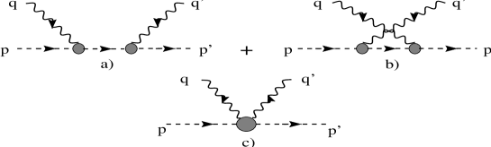
$\displaystyle{\cal M}^{\rm VCS}_{\pi^{\pm}}$ $\displaystyle=$ $\displaystyle{\cal A}+{\cal B},\qquad{\cal M}^{\rm VCS}_{\pi^{0}}={\cal A},$
$\displaystyle{\cal M}^{\rm VCS}_{K^{\pm}}$ $\displaystyle=$ $\displaystyle{\cal C}+{\cal D},\qquad{\cal M}^{\rm VCS}_{K^{0}}={\cal M}^{\rm VCS}_{\bar{K}^{0}}={\cal C}.$

In addition, we split ${\cal M}^{\rm VCS}$ into a Born (B) and a non-Born (NB) term which we construct such that they are separately gauge invariant, ${\cal M}^{\rm VCS}={\cal M}_{\rm B}^{\rm VCS}+{\cal M}_{\rm NB}^{\rm VCS}$ (see Fig.Β 1).

Refer to caption

Fig.Β 1.Β : Compton scattering amplitude: ${\rm a})$ and ${\rm b})$ pole graphs; ${\rm c})$ one-particle-irreducible contribution. All the building blocks are renormalized.

The result for the gauge-invariant generalized Born terms reads

$\displaystyle{\cal B}_{\rm B}$ $\displaystyle=$ $\displaystyle-2{\rm i}e^{2}F_{\pi}(q^{2})\left[\frac{\epsilon\cdot(2p+q)\epsilon^{\prime}\,{}^{\ast}\cdot p^{\prime}}{s-m_{\pi}^{2}}+\frac{\epsilon\cdot(2p^{\prime}-q)\epsilon^{\prime}\,{}^{\ast}\cdot p}{u-m_{\pi}^{2}}-\epsilon\cdot\epsilon^{\prime}\,{}^{\ast}\right],$ (3)
$\displaystyle{\cal D}_{\rm B}$ $\displaystyle=$ $\displaystyle-2{\rm i}e^{2}F_{K}(q^{2})\left[\frac{\epsilon\cdot(2p+q)\epsilon^{\prime}\,{}^{\ast}\cdot p^{\prime}}{s-m_{K}^{2}}+\frac{\epsilon\cdot(2p^{\prime}-q)\epsilon^{\prime}\,{}^{\ast}\cdot p}{u-m_{K}^{2}}-\epsilon\cdot\epsilon^{\prime}\,{}^{\ast}\right],$ (4)

where $F_{\pi(K)}$ is the charged pion (kaon) form factor. The gauge-invariant residual amplitude is given by

$\displaystyle{\cal A}_{\rm NB}$ $\displaystyle=$ $\displaystyle-{\rm i}e^{2}(q^{\prime}\cdot\epsilon q\cdot\epsilon^{\prime}\,{}^{\ast}-q\cdot q^{\prime}\epsilon\cdot\epsilon^{\prime}\,{}^{\ast})\frac{1}{8\pi^{2}F_{0}^{2}q\cdot q^{\prime}}\left[(m^{2}_{\pi}-t){\cal G}_{\pi}-\frac{1}{4}t{\cal G}_{K}\right],$ (5)
$\displaystyle{\cal B}_{\rm NB}$ $\displaystyle=$ $\displaystyle-{\rm i}e^{2}(q^{\prime}\cdot\epsilon q\cdot\epsilon^{\prime}\,{}^{\ast}-q\cdot q^{\prime}\epsilon\cdot\epsilon^{\prime}\,{}^{\ast})\left[-\frac{8(L_{9}^{r}+L_{10}^{r})}{F_{0}^{2}}-\frac{2m^{2}_{\pi}-t}{16\pi^{2}F_{0}^{2}q\cdot q^{\prime}}{\cal G}_{\pi}\right],$ (6)
$\displaystyle{\cal C}_{\rm NB}$ $\displaystyle=$ $\displaystyle{\rm i}e^{2}(q^{\prime}\cdot\epsilon q\cdot\epsilon^{\prime}\,{}^{\ast}-q\cdot q^{\prime}\epsilon\cdot\epsilon^{\prime}\,{}^{\ast})\frac{1}{16\pi^{2}F_{0}^{2}q\cdot q^{\prime}}\frac{t}{2}\left({\cal G}_{\pi}+{\cal G}_{K}\right),$ (7)
$\displaystyle{\cal D}_{\rm NB}$ $\displaystyle=$ $\displaystyle-{\rm i}e^{2}(q^{\prime}\cdot\epsilon q\cdot\epsilon^{\prime}\,{}^{\ast}-q\cdot q^{\prime}\epsilon\cdot\epsilon^{\prime}\,{}^{\ast})\left[-\frac{8(L_{9}^{r}+L_{10}^{r})}{F_{0}^{2}}-\frac{t}{32\pi^{2}F_{0}^{2}q\cdot q^{\prime}}{\cal G}_{K}\right],$ (8)

where $s$, $t$, and $u$ are the standard Mandelstam variables. In Eqs. (5) - (8) the function ${\cal G}_{\pi(K)}:={\cal G}(m^{2}_{\pi(K)},q^{2},q\cdot q^{\prime})$ corresponds to the pion (kaon) loop integral contributions, and is explicitly given in the appendix. We note that out of the 12 low-energy constants contained in ${\cal L}_{4}$ only the combination $L^{r}_{9}+L^{r}_{10}$ enters in our result, with the value $L^{r}_{9}+L^{r}_{10}=(1.43\pm 0.27)\times 10^{-3}$ being determined through the decay $\pi^{+}\to e^{+}\nu_{e}\gamma$.

4 Generalized Polarizabilities

Following the analysis of Ref. [12], the invariant VCS amplitude can be parametrized as

$$-{\rm i}{\cal M}=B_{1}F^{\mu\nu}F^{\prime}_{\mu\nu}+\frac{1}{4}B_{2}\left(P_{\mu}F^{\mu\nu}\right)\left(P^{\rho}F^{\prime}_{\rho\nu}\right)+\frac{1}{4}B_{3}\left(P^{\nu}q^{\mu}F_{\mu\nu}\right)\left(P^{\sigma}q^{\rho}F^{\prime}_{\rho\sigma}\right),$$ (9)

where $P_{\mu}=p_{\mu}+p^{\prime}_{\mu}$, $F^{\mu\nu}=-{\rm i}(q^{\mu}\varepsilon^{\nu}-q^{\nu}\varepsilon^{\mu})$ and $F^{\prime}_{\mu\nu}={\rm i}(q^{\prime}_{\mu}\varepsilon^{\prime}\,{}^{*}_{\nu}-q^{\prime}_{\nu}\varepsilon^{\prime}\,{}^{*}_{\mu})$. The structures of Eq. (9) are particularly simple when evaluated in the pion Breit frame (PBF) defined by $\mbox{\boldmath$P$}=\mbox{\boldmath$0$}$. In this frame, the structures $\mbox{\boldmath$E$}_{L}\cdot\mbox{\boldmath$E$}^{\prime}$, $\mbox{\boldmath$E$}_{T}\cdot\mbox{\boldmath$E$}^{\prime}$, and $\mbox{\boldmath$B$}\cdot\mbox{\boldmath$B$}^{\prime}$ appear. We now consider the limit $\omega^{\prime}\to 0$ of the non-Born amplitude ${\cal M}_{\rm NB}$, for which $B_{i\,{\rm NB}}\to b_{i\,{\rm NB}}$, and define three generalized dipole polarizabilities,

$\displaystyle 8\pi m_{\pi}\beta(q^{2})$ $\displaystyle\equiv$ $\displaystyle b_{1\,{\rm NB}},$ (10)
$\displaystyle 8\pi m_{\pi}\alpha_{T}(q^{2})$ $\displaystyle\equiv$ $\displaystyle-b_{1\,{\rm NB}}(q^{2})-\left(m_{\pi}^{2}-\frac{q^{2}}{4}\right)b_{2\,{\rm NB}}(q^{2}),$ (11)
$\displaystyle 8\pi m_{\pi}\alpha_{L}(q^{2})$ $\displaystyle\equiv$ $\displaystyle-b_{1\,{\rm NB}}(q^{2})-\left(m_{\pi}^{2}-\frac{q^{2}}{4}\right)\left[b_{2\,{\rm NB}}(q^{2})+q^{2}b_{3\,{\rm NB}}(q^{2})\right].$ (12)

We note that $[\mbox{\boldmath$B$}\cdot\mbox{\boldmath$B$}^{\prime}]_{\rm PBF}$ and $[\mbox{\boldmath$E$}_{L}\cdot\mbox{\boldmath$E$}^{\prime}]_{\rm PBF}$ are of ${\cal O}(\omega^{\prime})$ whereas $[\mbox{\boldmath$E$}_{T}\cdot\mbox{\boldmath$E$}^{\prime}]_{\rm PBF}={\cal O}(\omega^{\prime 2})$, i.e., that different powers of $\omega^{\prime}$ have been kept.

In ChPT up to ${\cal O}(p^{4})$, $b_{2\,{\rm NB}}(q^{2})=b_{3\,{\rm NB}}(q^{2})=0$, which leads to the relation

$$\alpha_{L}(q^{2})=\alpha_{T}(q^{2})=-\beta(q^{2}).$$ (13)

The explicit expressions for the polarizabilities read

$\displaystyle\alpha_{L}^{\pi^{\pm}}(q^{2})$ $\displaystyle=$ $\displaystyle\frac{e^{2}}{8\pi m_{\pi}}\left\{\frac{8\left(L_{9}^{r}+L_{10}^{r}\right)}{F_{0}^{2}}\right.$ (14)
$\displaystyle\left.-\frac{q^{2}}{m_{\pi}^{2}}\frac{1}{\left(4\pi F_{0}\right)^{2}}\left[J^{(0)^{\prime}}\left(\frac{q^{2}}{m^{2}_{\pi}}\right)+\frac{1}{2}\frac{m^{2}_{\pi}}{m^{2}_{K}}J^{(0)^{\prime}}\left(\frac{q^{2}}{m^{2}_{K}}\right)\right]\right\},$
$\displaystyle\alpha_{L}^{\pi^{0}}(q^{2})$ $\displaystyle=$ $\displaystyle\frac{e^{2}}{4\pi}\frac{1}{\left(4\pi F_{0}\right)^{2}m_{\pi}}\left[-\frac{1}{4}\frac{q^{2}}{m_{k}^{2}}J^{(0)^{\prime}}\left(\frac{q^{2}}{m^{2}_{K}}\right)+\left(1-\frac{q^{2}}{m_{\pi}^{2}}\right)J^{(0)^{\prime}}\left(\frac{q^{2}}{m_{\pi}^{2}}\right)\right],$
$\displaystyle\alpha_{L}^{K^{\pm}}(q^{2})$ $\displaystyle=$ $\displaystyle\frac{e^{2}}{8\pi m_{K}}\left\{\frac{8\left(L_{9}^{r}+L_{10}^{r}\right)}{F_{0}^{2}}\right.$ (16)
$\displaystyle\left.-\frac{q^{2}}{m_{K}^{2}}\frac{1}{\left(4\pi F_{0}\right)^{2}}\left[\frac{1}{2}\frac{m^{2}_{K}}{m^{2}_{\pi}}J^{(0)^{\prime}}\left(\frac{q^{2}}{m^{2}_{\pi}}\right)+J^{(0)^{\prime}}\left(\frac{q^{2}}{m^{2}_{K}}\right)\right]\right\},$
$\displaystyle\alpha_{L}^{K^{0}}(q^{2})$ $\displaystyle=$ $\displaystyle-\frac{e^{2}}{4\pi}\frac{1}{\left(4\pi F_{0}\right)^{2}}\frac{q^{2}}{4m_{K}^{3}}\left[\frac{m_{K}^{2}}{m_{\pi}^{2}}J^{(0)^{\prime}}\left(\frac{q^{2}}{m_{\pi}^{2}}\right)+J^{(0)^{\prime}}\left(\frac{q^{2}}{m^{2}_{K}}\right)\right],$ (17)

where the function $J^{(0)^{\prime}}(x)$ is given in the appendix. Note that the ${\cal L}_{4}$ low-energy constants enter only in the result for the charged particles.

The results for the generalized polarizabilities as function of $Q^{2}=-q^{2}$ are shown in Fig. 2. We made use of the numerical value $F_{0}\simeq F_{\pi}=92.4\,\mbox{MeV}$.

Refer to caption

Fig.Β 2.Β : ${\cal O}(p^{4})$ predictions for the generalized pion and kaon polarizabilities $\alpha_{L}(q^{2}=-Q^{2})$. The solid lines correspond to the total results, while the dotted lines result from pion-loop contributions, only.

At $q^{2}=0$, Eqs. (14)-(17) reduce to the RCS polarizabilities given by

$\displaystyle\alpha_{\pi^{\pm}}=-\beta_{\pi^{\pm}}$ $\displaystyle=$ $\displaystyle(2.72\pm 0.42)\times 10^{-4}\,\mbox{fm}^{3},$ (18)
$\displaystyle\alpha_{\pi^{0}}=-\beta_{\pi^{0}}$ $\displaystyle=$ $\displaystyle-0.50\times 10^{-4}\,\mbox{fm}^{3},$ (19)
$\displaystyle\alpha_{K^{\pm}}=-\beta_{K^{\pm}}$ $\displaystyle=$ $\displaystyle(0.74\pm 0.12)\times 10^{-4}\,\mbox{fm}^{3},$ (20)
$\displaystyle\alpha_{K^{0}\,(\bar{K}^{0})}=\beta_{K^{0}\,(\bar{K}^{0})}$ $\displaystyle=$ $\displaystyle 0.$ (21)

In Tabs. 1 and 2 we collect the available experimental and theoretical results for the RCS polarizabilities. We note that the ChPT predictions are remarkably smaller compared to the experimental values and the other theoretical results.

reaction $\gamma p\rightarrow\gamma\pi^{+}n$ $\pi^{-}A\rightarrow\pi^{-}A\gamma$
$\alpha_{\pi^{\pm}}$ $20\pm 12\,$ [13] $6.8\pm 1.4\,$ [14]
$\beta_{\pi^{\pm}}$ $-$ $-7.1\pm 2.8\pm 1.8\,$ [15]
$\alpha_{\pi^{\pm}}+\beta_{\pi^{\pm}}$ $-$ $1.4\pm 3.1\pm 2.5\,$ [15]
Table 1.Β : Experimental predictions for the pion polarizabilities in units of $10^{-4}\,\mbox{fm}^{3}$.
chiral QM nonrel. QM NJL ChPT QCM
$\alpha_{\pi^{\pm}}$ $8.0$ $0.05$ $10.5-12.5$ $2.4\pm 0.5$ $3.63$
$\beta_{\pi^{\pm}}$ $-7.8$ $-$ $-(10.3-11.8)$ $-2.1\pm 0.5$ $-2.41$
$\alpha_{\pi^{0}}$ $-$ $-$ $-$ $-0.35\pm 0.10$ $0.74$
$\beta_{\pi^{0}}$ $-$ $-$ $-$ $1.50\pm 0.20$ $-0.30$
$\alpha_{K^{\pm}}$ $9.7$ $-$ $-$ $0.64\pm 0.1$ $2.28$
$\beta_{K^{\pm}}$ $-4.4$ $-$ $-$ $-$ $-1.31$
Table 2.Β : Theoretical predictions for the pion and kaon polarizabilities (in units of $10^{-4}\,\mbox{fm}^{3}$) within different models, like chiral quark model (QM) [16], nonrelativistic quark model (nonrel. QM) [17], Nambu-Jona-Lasinio (NJL) model [18], ChPT [19], and quark confinement model (QCM) [20].

5 Electron-Meson Bremsstrahlung

VCS off the pseudoscalar meson octet can be accessed experimentally via the electron-meson bremsstrahlung reaction. Such events are presently under analysis in the SELEX-E781 experiment [2], where negative high energy pions of $\sim$ 600 GeV are inelastically scattered off atomic electrons, $\pi^{-}(p)e^{-}(k)\to\pi^{-}(p^{\prime})e^{-}(k^{\prime})\gamma(q^{\prime}).$ The amplitude for this reaction is given by the sum of the Bethe-Heitler (BH) and the full virtual Compton scattering (FVCS) contributions, ${\cal M}={\cal M}_{\rm BH}+{\cal M}_{\rm FVCS}$ (see Fig. 3).

Refer to caption

Fig.Β 3.Β : Bethe-Heitler and FVCS diagrams.

The BH diagrams correspond to the emission of the final photon from the electron in the initial or final states, and involves only on-shell information of the target, like the mass, the charge and the electromagnetic form factor. The explicit expression for the BH term reads

$\displaystyle{\cal M}_{\rm BH}$ $\displaystyle=$ βˆ’i​e3β€‹Ο΅ΞΌβ€²β£βˆ—r2​u¯​(kβ€²,skβ€²)​(γμ​qβ€²β‹…Ξ³+2​k′⁣μ2​kβ€²β‹…q′​γν+γν​qβ€²β‹…Ξ³β€‹Ξ³ΞΌβˆ’2​kΞΌ2​kβ‹…qβ€²)​u​(k,sk)isuperscript𝑒3subscriptsuperscriptitalic-Ο΅β€²βˆ—πœ‡superscriptπ‘Ÿ2¯𝑒superscriptπ‘˜β€²subscript𝑠superscriptπ‘˜β€²β‹…superscriptπ›Ύπœ‡superscriptπ‘žβ€²π›Ύ2superscriptπ‘˜β€²πœ‡β‹…2superscriptπ‘˜β€²superscriptπ‘žβ€²superscriptπ›Ύπœˆsuperscriptπ›Ύπœˆβ‹…superscriptπ‘žβ€²π›Ύsuperscriptπ›Ύπœ‡2superscriptπ‘˜πœ‡β‹…2π‘˜superscriptπ‘žβ€²π‘’π‘˜subscriptπ‘ π‘˜\displaystyle-\frac{{\rm i}e^{3}\epsilon^{\prime\ast}_{\mu}}{r^{2}}\bar{u}(k^{\prime},s_{k^{\prime}})\left(\frac{\gamma^{\mu}q^{\prime}\cdot\gamma+2k^{\prime\mu}}{2k^{\prime}\cdot q^{\prime}}\gamma^{\nu}+\gamma^{\nu}\frac{q^{\prime}\cdot\gamma\gamma^{\mu}-2k^{\mu}}{2k\cdot q^{\prime}}\right)u(k,s_{k}) (22)
$\displaystyle\times\left(p+p^{\prime}\right)_{\nu}F_{\pi}(r^{2}),$

where $r^{\mu}=p^{\mu}-p^{\prime}\,{}^{\mu}$ is the four-momentum transfer to the target.

In the one-photon exchange approximation, the FVCS amplitude is proportional to the VCS amplitude, and reads

$\displaystyle{\cal M}^{\rm FVCS}$ $\displaystyle=$ βˆ’i​e3q2​u¯​(kβ€²,skβ€²)​γμ​u​(k,sk)​ϡν′​ℳVCSΞΌβ€‹Ξ½βˆ—.isuperscript𝑒3superscriptπ‘ž2¯𝑒superscriptπ‘˜β€²subscript𝑠superscriptπ‘˜β€²subscriptπ›Ύπœ‡π‘’π‘˜subscriptπ‘ π‘˜subscriptsuperscriptitalic-Ο΅β€²πœˆsuperscriptsuperscriptsubscriptβ„³VCSπœ‡πœˆ\displaystyle-\frac{{\rm i}e^{3}}{q^{2}}\bar{u}(k^{\prime},s_{k^{\prime}})\gamma_{\mu}u(k,s_{k})\epsilon^{\prime}_{\nu}\,{}^{*}{\cal M}_{\rm VCS}^{\mu\nu}. (23)

The differential cross section is then obtained from the coherent sum of the BH and FVCS contributions. In the limit $\omega^{\prime}\rightarrow 0$, the interference of the BH and Born terms with the leading contribution of the residual VCS amplitude contains information on the generalized polarizabilities.

Refer to caption

Fig.Β 4.Β : Differential cross sections for the charged pions. Full lines: total results; dashed lines: BH and Born contributions; dotted lines: background contribution corresponding to the coherent sum of the BH and Born terms; dashed-dotted lines: total results with the residual VCS contribution calculated without taking into account the $q^{2}$ dependence of the polarizability and using $\alpha_{\pi}=10\times 10^{-4}\,\mbox{fm}^{3}$.

In Fig. 4 we show the differential cross section for the charged pions in a kinematical regime which can be accessed by the SELEX experiment [2]: $s=(p+k)^{2}=0.68\,\mbox{GeV}^{2}$, $s_{1}=(k^{\prime}+q^{\prime})^{2}=0.154\,\mbox{GeV}^{2}$, $s_{2}=(p^{\prime}+q^{\prime})^{2}=0.2117\,\mbox{GeV}^{2}$, $r^{2}=(p-p^{\prime})^{2}=-0.0947\,\mbox{GeV}^{2}$. The main contribution to the total cross section is given by the interference between the Born and the BH terms. This interference term is positive for $\pi^{+}$ and negative for $\pi^{-}$ since the BH term is proportional to the pion form factor. The effects of the polarizabilities correspond to the difference between the total result (solid lines) and the background contribution of the BH and Born terms (dotted lines). In addition, the effects due to the $q^{2}$ dependence of the polarizability can be seen by comparing the full lines with the dashed-dotted lines, where the contribution of the residual VCS amplitude is calculated using the constant value of $\alpha_{\pi}=10\times 10^{-4}\,\mbox{fm}^{3}$.

6 Summary

We have calculated the invariant amplitude for VCS off the pseudoscalar meson octet in ChPT at ${\cal O}(p^{4})$. This amplitude was split into a generalized Born and an non-Born term, where each term was separately gauge invariant. In the limit $\omega^{\prime}\rightarrow 0$, the non-Born contribution can be parametrized in terms of generalized polarizabilities. We used for the definition of these quantities a covariant approach interpreted in the pion Breit frame. In the framework of ChPT at ${\cal O}(p^{4})$, we found that the momentum dependence of the generalized kaon and pion polarizabilities is entirely given in terms of the mass and the decay constant of the meson. Finally, we have investigated the possibility to extract information about the generalized pion polarizabilities through the electron-pion bremsstrahlung reaction. This reaction receives a large background contribution from the Bethe-Heitler and Born terms, and very high precision measurements are necessary to disentangle the effects of the polarizabilities.

A The loop function ${\cal G}(m^{2},q^{2},q\cdot q^{\prime})$

The function ${\cal G}(m^{2},q^{2},q\cdot q^{\prime})$ is defined via

$${\cal G}(m^{2},q^{2},q\cdot q^{\prime})=1+\frac{m^{2}}{q\cdot q^{\prime}}\left[J^{(-1)}(a)-J^{(-1)}(b)\right]-\frac{q^{2}}{2q\cdot q^{\prime}}\left[J^{(0)}(a)-J^{(0)}(b)\right],$$ (24)

where

$$J^{(n)}(x):=\int_{0}^{1}{\rm d}yy^{n}\ln[1+x(y^{2}-y)-{\rm i}0^{+}]$$

and

$$a:=\frac{q^{2}}{m},\quad b:=\frac{q^{2}-2q\cdot q^{\prime}}{m^{2}}.$$

The functions $J^{(0)}$ and $J^{(-1)}$ can be expressed as

$\displaystyle J^{(0)}(x)$ $\displaystyle=$ $\displaystyle\left\{\begin{array}[]{ll}-2-\sigma\ln\left(\frac{\sigma-1}{\sigma+1}\right)&(x<0),\\ -2+2\sqrt{\frac{4}{x}-1}\,\mbox{arccot}\left(\sqrt{\frac{4}{x}-1}\right)&(0\leq x<4),\\ -2-\sigma\ln\left(\frac{1-\sigma}{1+\sigma}\right)-{\rm i}\pi\sigma&(4<x),\end{array}\right.$
$\displaystyle J^{(-1)}(x)$ $\displaystyle=$ $\displaystyle\left\{\begin{array}[]{ll}\frac{1}{2}\ln^{2}\left(\frac{\sigma-1}{\sigma+1}\right)&(x<0),\\ -\frac{1}{2}\arccos^{2}\left(1-\frac{x}{2}\right)&(0\leq x<4),\\ \frac{1}{2}\ln^{2}\left(\frac{1-\sigma}{1+\sigma}\right)-\frac{\pi^{2}}{2}+{\rm i}\pi\ln\left(\frac{1-\sigma}{1+\sigma}\right)&(4<x),\end{array}\right.$

with

$$\sigma(x)=\sqrt{1-\frac{4}{x}},\quad x\notin[0,4].$$

The function $J^{(0)^{\prime}}(x)$ is given by

$$J^{(0)^{\prime}}(x)=\frac{1}{x}\left[1-\frac{2}{x\sigma}\ln\left(\frac{\sigma-1}{\sigma+1}\right)\right]=\frac{1}{x}\left[1+2J^{(-1)^{\prime}}(x)\right],\qquad x<0.$$ (27)

References

  • [1] P.A.M. Guichon, G.Q. Liu, and A.W. Thomas, Nucl. Phys. A591, 606 (1995)
  • [2] M.A. Moinester et al., Baryons ’98, edited by D.W. Menze and B. Metsch (World Scientific, Singapore, 1997), and hep-ex/9903039 (1999); A. Ocherashvili, PhD thesis, Tel Aviv University, 2000
  • [3] S. Bellucci, Proc. of the Workshop Chiral Dynamics: Theory and Experiment, Cambridge, MA, 1994, edited by M. Bernstein and Barry R. Holstein (Springer-Verlag, Berlin, 1995), and hep-ph/9508282
  • [4] R. Beck et al., Measurement of the $\pi^{+}$ meson polarizability, MAMI proposal (1994)
  • [5] T. Gorringe (spokesman), TRIUMF Expt. E838 (1998)
  • [6] M.A. Moinester and V. Steiner, Proc. of the Charles U./JINR and International U. (Dubna) CERN Compass Summer School, 1997, Prague, ed. M. Chavleishvili and M. Finger, and hep-ex/9801011.
  • [7] J. Gasser and H. Leutwyler, Ann. Phys. 158, 142 (1984)
  • [8] J. Gasser and H. Leutwyler, Nucl. Phys. B250, 465 (1985)
  • [9] J. Goldstone, Nuovo Cim. 19, 154 (1961)
  • [10] S. Weinberg, Physica 96A, 327 (1979)
  • [11] J.D. Bjorken and S. Drell, Relativistic Quantum Mechanics (McGraw-Hill, New York, 1964)
  • [12] C. Unkmeir, S. Scherer, A.I. L’vov, and D. Drechsel, Phys. Rev. D 61, 034002 (2000)
  • [13] T.A. Aibergenov et al., Czech. J. Phys. B36, 948 (1986)
  • [14] Y.M. Antipov et al., Phys. Lett. B 121, 445 (1983)
  • [15] Y.M. Antipov et al., Z. Phys. C 26, 495 (1985)
  • [16] M.K. Volkov and D. Ebert, Sov. J. Nucl. Phys. 34, 104 (1981); D. Ebert, M.K. Volkov, and T. Feldmann, Int. J. Mod. Phys. A12, 4399 (1997)
  • [17] F. Schoeberl and H. Leeb, Phys. Lett. B 166, 355 (1986)
  • [18] V. Bernard and D. Vautherin, Phys. Rev. D 40, 1615 (1989)
  • [19] U. BΓΌrgi, Phys. Lett. B 377, 1 (1996); S. Bellucci, J. Gasser, and M.E. Sainio, Nucl. Phys. B423, 80 (1994); F. Guerrero and J. Prades, Phys. Lett. B 405, 341 (1997)
  • [20] M.A. Ivanov and T. Mizutani, Phys.Β Rev.Β D 45, 1580 (1992)