On the quantum loop weak interaction corrections at high energies

D. PALLE
Zavod za teorijsku fiziku
Institut Rugjer Boลกkoviฤ‡
P. O. Box 180, 10002 Zagreb, CROATIA
This work was supported by the Ministry of Science and Technology of the Republic of Croatia No. 00980103.
Abstract:

We perform comparative analyses of quantum loop corrections to some observationally important two- and three-point Green functions within two distinct symmetry-breaking mechanisms. It appears that the existing high-energy data, neutrino experiments and present astrophysical and cosmological constraints strongly disfavour the Higgs mechanism, while the introduction of the noncontractible space as a symmetry-breaking mechanism can resolve all known problems and puzzles of fundamental interactions.

1 Introduction and motivation

The current and commonly accepted wisdom in particle physics relies strongly on the formalism of quantum field theory of unitary gauge symmetries of the Standard Model (SM). The success of the perturbative calculations and their agreement with measurements at low and very high energies, represent the milestone of our confidence into the SM. However, recent developments in theoretical and experimental particle physics are far from being considered satisfactory.

Although there is great discontent with the SM, the SUSY, GUT, etc extensions of the SM are also based on the Higgs mechanism, thus preserving all of its bad features: fermion masses are free parameters, the introduction of new Higgs scalars to resolve small neutrino masses, unclear source of fermion mixings, production of the large cosmological constant, etc. Our motivation to change the symmetry-breaking mechanism is based on the arguments related to the mathematical inconsistency of the SM [1], namely the SU(2) global anomaly and the ultraviolet (UV) singularity. The mathematically consistent theory (called BY in [1]) violates lepton-number conservation and contains three light and three heavy Majorana neutrinos, while the finite UV scale is fixed by the weak interaction scale, explaining simultaneously broken conformal, gauge and discrete symmetries. The dimensionality and noncontractibility of the physical space should be the only assumption that suffices to unify strong and electroweak forces realized as hidden local symmetries within the SU(3) conformal scheme.

LSND and SuperKamiokande data refer clearly to the existence of massive neutrinos and the neutrino flavour mixing. Present fits to neutrino data require higher masses and mixing angles that are close to the estimates in [1]. Owing to the absence of the Higgs scalars, one is able to show within the BY theory that heavy neutrinos of mass ${\cal O}(100TeV)$ could be candidate particles as cold dark matter and their lifetimes ๐’ชโ€‹(1025โ€‹s)๐’ชsuperscript1025๐‘ {\cal O}(10^{25}s) could resolve the problem of the cosmological diffuse photon background [2]. The first nonvanishing contribution to the CDM particle-nucleon scattering appears at two loops in the strong coupling and DAMA data could be quantitatively understood [3].

We have also investigated the finite scale effect on the running coupling in perturbative QCD [4]. The absence of asymptotic freedom, limฮผโ†’โˆžฮฑsฮ›โ€‹(ฮผ)โ‰ 0subscriptโ†’๐œ‡superscriptsubscript๐›ผ๐‘ ฮ›๐œ‡0\lim_{\mu\rightarrow\infty}\alpha_{s}^{\Lambda}(\mu)\neq 0, and the enhancement of the strong coupling that starts in the vicinity of the weak interaction scale, are large deviations from the SM. In this paper we analyse quantum loop weak corrections and the differences between the SM and the BY theory. In the next chapter we define renormalization procedures and in the last chapter we give the results with remarks and discussions of recent high-energy data at colliders.

2 Renormalisation

In this section we define renormalisation conditions and Green functions in order to comparatively analyse the SM and the BY theory. Since the masses of heavy neutrinos in the BY are at least a few TeV [2] and the masses of light neutrinos are negligible in comparison with charged lepton masses, we perform the calculations in the BY with massless neutrinos, thus with no lepton-number violation.

Effectively, we perform the calculations with the Higgs scalar of the SM and with the UV cut-off and without the Higgs scalar, as in the BY theory. The spontaneously broken electroweak theories are renormalisable theories even if there is no Higgs scalar because in the closed set of asymptotic fields that forms the BRST transformations, the Higgs field is absent [5, 1].

We choose renormalisation conditions for the vector gauge boson fields in the manner to preserve the position and the residue of the mass singularity of the respective propagator [6] with particular emphasis on the mixing of neutral fields:

$\displaystyle\Delta(q^{2})^{-1}\equiv q^{2}-M_{V}^{2}+\Sigma^{R}(q^{2}),$ (1)
$\displaystyle\Sigma^{R}_{i}(M_{i}^{2})=0,\ \frac{d\Sigma^{R}_{i}}{dq^{2}}(q^{2}=M_{i}^{2})=0,$
$\displaystyle\Sigma^{R}_{i}(q^{2})=\Sigma^{U}_{i}(q^{2})+\Sigma^{C}_{i}(q^{2}),\ i=Z,W,$
$\displaystyle\Sigma^{C}_{i}(q^{2})=\delta M^{2}_{i}+Z_{i}(M^{2}_{i}-q^{2}),$
$\displaystyle\Sigma^{U}_{i}(M^{2}_{i})+\delta M^{2}_{i}=0,$
$\displaystyle\frac{d\Sigma^{U}_{i}}{dq^{2}}(q^{2}=M^{2}_{i})-Z_{i}=0,$ (2)
$\displaystyle\Sigma^{R}_{ZA}(0)=0,\ \Sigma^{R}_{ZA}(M_{Z}^{2})=0,$
$\displaystyle\Sigma^{R}_{ZA}(q^{2})=\Sigma^{U}_{ZA}(q^{2})+\Sigma^{C}_{ZA}(q^{2}),$
$\displaystyle\Sigma^{ZA}_{C}(q^{2})=Z^{1/2}_{ZA}(M^{2}_{Z}-q^{2})-Z^{1/2}_{AZ}q^{2},$
$\displaystyle\Sigma^{U}_{ZA}(M^{2}_{Z})-M^{2}_{Z}Z^{1/2}_{AZ}=0,$
$\displaystyle\Sigma^{U}_{ZA}(0)+M^{2}_{Z}Z^{1/2}_{ZA}=0,$ (3)
$\displaystyle\Sigma^{R}_{A}(0)=0,\frac{d\Sigma^{R}_{A}}{dq^{2}}(q^{2}=0)=0,$
$\displaystyle\Sigma^{R}_{A}(q^{2})=\Sigma^{U}_{A}(q^{2})+\Sigma^{C}_{A}(q^{2}),$
$\displaystyle\Sigma^{C}_{A}(q^{2})=-2q^{2}Z^{1/2}_{AA},$
$\displaystyle\frac{d\Sigma^{U}_{A}}{dq^{2}}(q^{2}=0)-2Z^{1/2}_{AA}=0.$ (4)

Similarly, one has to impose renormalisation conditions on the fermion propagators with mixing [7] and the most natural choice for the mixing operators is $\Sigma^{R}_{ij}(m_{i}^{2})=0$ and $\Sigma^{R}_{ij}(m_{j}^{2})=0$, i,j=flavour indices. In the calculation of the boson propagators we neglect the fermion mixing effect, because it is numerically unimportant.

We have to mention that the above renorm conditions differ markedly from those in Ref.[8]. The conditions of Bรถhm et al do not fulfil the requirements for the propagator to match the free-field mass singularity structure. It is not clear how their renorm conditions can remove UV singularity in the structure $C_{UV}^{\infty}(k^{2}-M_{V}^{2})$ of the propagator. As a consequence, one cannot use their renormalised propagators directly in the evaluation of the observables, such as the effective weak mixing angle. The result of the unsuitable renorm conditions in [8] is the appearance of a completely spurious term for the quantum correction to the effective weak-mixing angle [9]

MW2โ€‹sW2subscriptsuperscript๐‘€2๐‘Šsubscriptsuperscript๐‘ 2๐‘Š\displaystyle M^{2}_{W}s^{2}_{W} $\displaystyle=$ $\displaystyle\frac{\pi\alpha_{e}}{\sqrt{2}G_{\mu}}\frac{1}{1-\bigtriangleup r},$
$\displaystyle\bigtriangleup r$ $\displaystyle=$ ฮฃWRโ€‹(0)MW2+ฮฑe4โ€‹ฯ€โ€‹sW2โ€‹(6+7โˆ’4โ€‹sW22โ€‹sW2โ€‹lnโกcW2),subscriptsuperscriptฮฃ๐‘…๐‘Š0subscriptsuperscript๐‘€2๐‘Šsubscript๐›ผ๐‘’4๐œ‹subscriptsuperscript๐‘ 2๐‘Š674subscriptsuperscript๐‘ 2๐‘Š2subscriptsuperscript๐‘ 2๐‘Šsubscriptsuperscript๐‘2๐‘Š\displaystyle\frac{\Sigma^{R}_{W}(0)}{M^{2}_{W}}+\frac{\alpha_{e}}{4\pi s^{2}_{W}}(6+\frac{7-4s^{2}_{W}}{2s^{2}_{W}}\ln c^{2}_{W}),
$\displaystyle(\bigtriangleup r)_{top}$ $\displaystyle\approx$ โˆ’ฮฑe4โ€‹ฯ€โ€‹3โ€‹cW24โ€‹sW4โ€‹mt2MW2,subscript๐›ผ๐‘’4๐œ‹3subscriptsuperscript๐‘2๐‘Š4subscriptsuperscript๐‘ 4๐‘Šsubscriptsuperscript๐‘š2๐‘กsubscriptsuperscript๐‘€2๐‘Š\displaystyle-\frac{\alpha_{e}}{4\pi}\frac{3c^{2}_{W}}{4s^{4}_{W}}\frac{m^{2}_{t}}{M^{2}_{W}}, (5)
sWsubscript๐‘ ๐‘Š\displaystyle s_{W} $\displaystyle\equiv$ $\displaystyle\sin\theta_{W},\ c_{W}\equiv\cos\theta_{W}.$

Further numerical comparison of two renorm schemes is given in the next section.

It is very well known that the on-shell renorm conditions to the electron-photon vertex remove any further divergences of the electroweak vertices [6, 8]. However, we choose two conditions for the vertices under our study [9]:

$\displaystyle F^{Zf}_{V}(0)_{weak}=F^{Zf}_{A}(0)_{weak}=0.$ (6)

For our purpose, it will suffice to compare quantum corrections for the SM and the BY theory.

Although the renorm conditions for the SM and the BY theory should be the same, the differences between the renorm procedures are (1) presence (absence) of the Higgs scalar, (2) absence (presence) of the UV cut-off in the scalar Green functions. The Green functions with the UV cut-off should preserve the following characteristics: (1) the real parts should be defined after Wickโ€™s rotation and integration in the spacelike region up to the covariant cut-off and analytically continued on the Riemann sheets above the threshold in the timelike region, matching the standard Green functions in the limit $\Lambda=\infty$, (2) because of the broken scale invariance for $\Lambda<\infty$, one has to symmetrise the Green function over the masses and external momenta to preserve the exchange symmetry properties of the standard regularised functions (see Appendix B).

3 Results and discussion

Following the procedures described in the preceding section, one can evaluate renormalised gauge boson propagators in the SM and the BY theory (see Appendix A for the unrenormalised functions).

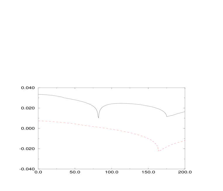
At first place, in Fig. 1 we display Z and W renorm propagators of the SM in order to make a comparison with the renorm scheme of Bรถhm et al (see Figs. 10 and 11 of Ref. [8]).

One can see that the difference between the two schemes is substantial and the contribution of the correct W gauge boson renorm propagator to the effective weak-mixing angle is dominated by the gauge boson loops without any enhancement due to the heavy top quark mass $\bigtriangleup r=-0.0413$ (parameters of this paper,see below).

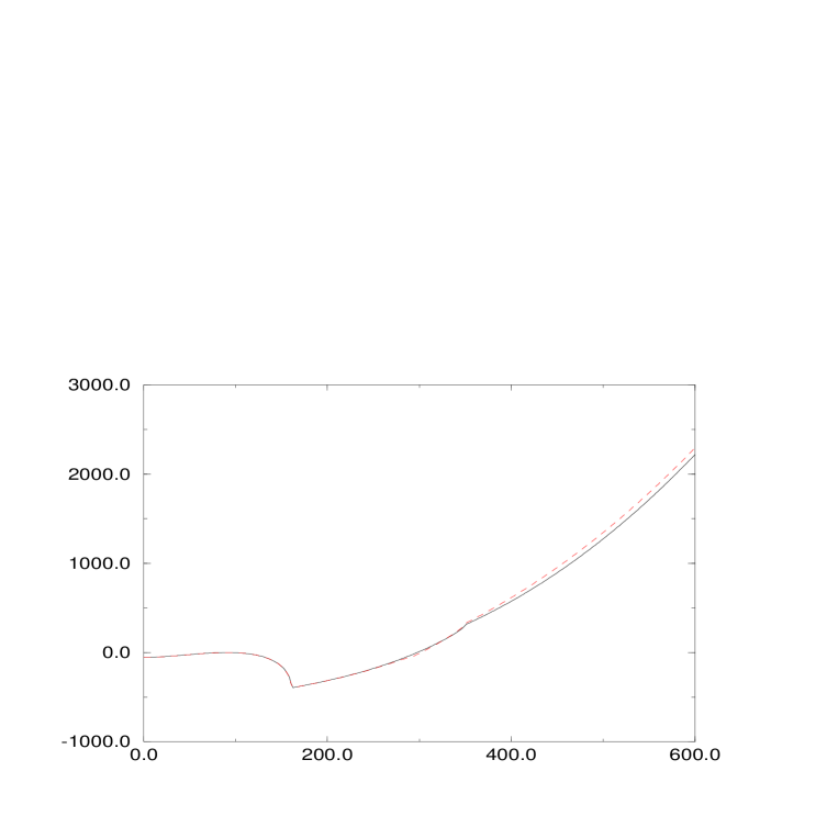
With the set of parameters

$\displaystyle M_{H}$ $\displaystyle=$ 200โ€‹Gโ€‹eโ€‹V,MW=80.44โ€‹Gโ€‹eโ€‹V,MZ=91.19โ€‹Gโ€‹eโ€‹V,ms=0.16โ€‹Gโ€‹eโ€‹V,formulae-sequence200๐บ๐‘’๐‘‰subscript๐‘€๐‘Š80.44๐บ๐‘’๐‘‰formulae-sequencesubscript๐‘€๐‘91.19๐บ๐‘’๐‘‰subscript๐‘š๐‘ 0.16๐บ๐‘’๐‘‰\displaystyle 200GeV,\ M_{W}=80.44GeV,\ M_{Z}=91.19GeV,\ m_{s}=0.16GeV,
$\displaystyle m_{c}$ $\displaystyle=$ $\displaystyle 2GeV,\ m_{b}=4.5GeV,\ m_{t}=175GeV,\ \Lambda=326GeV,$

in Fig. 2 we draw the Z-boson renormalised propagators of the SM and the BY theory to make a direct comparison (dependence on the Higgs scalar mass does not influence essentially the result).

Refer to caption
Figure 1: Solid [dashed] line denotes $\Sigma^{R}_{W}(p^{2})/(p^{2}-M_{W}^{2})$ [$\Sigma^{R}_{Z}(p^{2})/(p^{2}-M_{Z}^{2})$] vs. p(GeV); parameters as in Ref. [8].
Refer to caption
Figure 2: Solid [dashed] line denotes $\Sigma^{R}_{Z}(p^{2})_{\Lambda}$ [$\Sigma^{R}_{Z}(p^{2})_{\infty}$](GeV2) vs. p (GeV).

One can notice that a substantial difference appears and grows starting from the scale $p\simeq 400GeV$.

Recently it has been reported that there is a deviation of the weak charge SM prediction from the measurements of parity-nonconservation in Cs [10]. The BY theory evidently cannot improve the situation; however, it seems that an additional atomic-structure calculation can explain this discrepancy [11].

In a similar fashion we compare quantum loop weak corrections to the vector and axial-vector couplings of heavy quarks. With the unrenormalised vertices of Append. A and Green functions of Append. B, the renorm procedure leads us to the following results:

$\displaystyle v_{f}$ $\displaystyle=$ $\displaystyle v_{f}^{0}+F^{Zf}_{V}(weak)+...,$ (7)
$\displaystyle a_{f}$ $\displaystyle=$ $\displaystyle a_{f}^{0}+F^{Zf}_{A}(weak)+...,$ (8)
$\displaystyle v_{f}^{0}$ $\displaystyle=$ (If3โˆ’2โ€‹sW2โ€‹Qf)/2โ€‹sWโ€‹cW,af0=If3/2โ€‹sWโ€‹cW.subscriptsuperscript๐ผ3๐‘“2subscriptsuperscript๐‘ 2๐‘Šsubscript๐‘„๐‘“2subscript๐‘ ๐‘Šsubscript๐‘๐‘Šsuperscriptsubscript๐‘Ž๐‘“0subscriptsuperscript๐ผ3๐‘“2subscript๐‘ ๐‘Šsubscript๐‘๐‘Š\displaystyle(I^{3}_{f}-2s^{2}_{W}Q_{f})/2s_{W}c_{W},\ a_{f}^{0}=I^{3}_{f}/2s_{W}c_{W}.
s๐‘ \sqrt{s}(GeV) 100 150 200 250 400 550 700 850
$10^{3}\cdot(F^{Zc}_{V}(\Lambda)-F^{Zc}_{V}(\infty))$ 0.44 0.49 0.60 0.77 5.60 7.75 12.29 19.10
$10^{3}\cdot(F^{Zc}_{A}(\Lambda)-F^{Zc}_{A}(\infty))$ 0.43 0.47 0.58 0.74 5.39 7.28 11.83 18.16
Table 1: Weak corrections to the Z-c quark vertex.
s๐‘ \sqrt{s}(GeV) 100 150 200 250 400 550 700 850
$10^{3}\cdot(F^{Zb}_{V}(\Lambda)-F^{Zb}_{V}(\infty))$ -1.95 -0.93 -0.56 -0.38 -0.28 -1.43 -6.56 -7.71
$10^{3}\cdot(F^{Zb}_{A}(\Lambda)-F^{Zb}_{A}(\infty))$ -1.19 -0.61 -0.38 -0.26 -0.19 -1.98 -7.89 -8.65
Table 2: Weak corrections to the Z-b quark vertex.
s๐‘ \sqrt{s}(GeV) 400 550 700 850
$10^{3}\cdot(F^{Zt}_{V}(\Lambda)-F^{Zt}_{V}(\infty))$ -2.31 1.08 12.15 16.03
$10^{3}\cdot(F^{Zt}_{A}(\Lambda)-F^{Zt}_{A}(\infty))$ -6.30 -1.88 11.90 16.15
Table 3: Weak corrections to the Z-t quark vertex.

Loop corrections to the weak couplings are two orders of magnitude smaller than the tree level values, and significant differences between the SM and the BY grow after the scale sโ‰ƒ400โ€‹Gโ€‹eโ€‹Vsimilar-to-or-equals๐‘ 400๐บ๐‘’๐‘‰\sqrt{s}\simeq 400GeV. One should also remember that any effective electroweak vertex with quarks also contains the QCD correction factor (higher-order corrections could be found in [12])

|VEโ€‹W+Qโ€‹Cโ€‹Dโ€‹(q2)|2=|VEโ€‹Wโ€‹(q2)|2โ€‹[1+ฮฑsโ€‹(q2)ฯ€+๐’ชโ€‹(ฮฑs2โ€‹(q2))].superscriptsubscript๐‘‰๐ธ๐‘Š๐‘„๐ถ๐ทsuperscript๐‘ž22superscriptsubscript๐‘‰๐ธ๐‘Šsuperscript๐‘ž22delimited-[]1subscript๐›ผ๐‘ superscript๐‘ž2๐œ‹๐’ชsubscriptsuperscript๐›ผ2๐‘ superscript๐‘ž2\displaystyle|V_{EW+QCD}(q^{2})|^{2}=|V_{EW}(q^{2})|^{2}[1+\frac{\alpha_{s}(q^{2})}{\pi}+{\cal O}(\alpha^{2}_{s}(q^{2}))].

The presented numerical results, together with our previous work, allow us to make a concluding discussion and observations: (1) the difference between the SM and BY weak corrections to the weak couplings of heavy quarks becomes effective at the rather large scale sโ‰ƒ400โ€‹Gโ€‹eโ€‹Vsimilar-to-or-equals๐‘ 400๐บ๐‘’๐‘‰\sqrt{s}\simeq 400GeV; (2) the observed nonresonant enhancement at HERA could be attributed to the QCD enhacement factor (1+ฮฑsฮ›โ€‹(p2)ฯ€)/(1+ฮฑsโˆžโ€‹(p2)ฯ€)1superscriptsubscript๐›ผ๐‘ ฮ›superscript๐‘2๐œ‹1superscriptsubscript๐›ผ๐‘ superscript๐‘2๐œ‹(1+\frac{\alpha_{s}^{\Lambda}(p^{2})}{\pi})/(1+\frac{\alpha_{s}^{\infty}(p^{2})}{\pi}) to the squared electroweak couplings of quarks [13] starting at $p\simeq 200GeV$; (3) a similar effect one expects at lepton colliders only for the jet production channel; this nonresonant enhancement is probably observed at LEP 2 [14]; (4) a clear signal at hadron high-energy colliders should come from the enhancement of the amplitude owing to the factor ฮฑsฮ›โ€‹(ฮผ)/ฮฑsโˆžโ€‹(ฮผ)superscriptsubscript๐›ผ๐‘ ฮ›๐œ‡superscriptsubscript๐›ผ๐‘ ๐œ‡\alpha_{s}^{\Lambda}(\mu)/\alpha_{s}^{\infty}(\mu) [15]; one could easily check that parton distributions are not very much affected by the stronger ฮฑssubscript๐›ผ๐‘ \alpha_{s}: there is a very small enhancement for small x and a very small suppression for large x [16], thus it is very difficult to find it in experimental data; (5) Run 2 of TeVatron, together with a new HERA run, are capable to resolve the existence and nature of this QCD effect; (6) it is not excluded that deviations of the electroweak couplings could be measured at TeVatron [17]; (7) it has been shown that the Einstein-Cartan nonsingular cosmology can solve the problem of the cosmic mass density, cosmological constant problem [18] and the primordial mass density fluctuation [19] without the introduction of the scalar (inflaton) field; (8) to conclude, one can say that the theory of vacuum and the Higgs mechanism is like a modern theory of ether, and it is natural to expect that Nature should choose only a mathematically consistent theory to describe the physical laws.

4 Appendix A

In this appendix we summarise unrenormalised gauge boson self energies and unrenormalised vector and axial-vector Z-boson-heavy quark vertices (โ€™t Hooft-Feynman gauge):

ฮฃAUโ€‹(s)subscriptsuperscriptฮฃ๐‘ˆ๐ด๐‘ \displaystyle\Sigma^{U}_{A}(s) $\displaystyle=$ $\displaystyle\frac{\alpha_{e}}{4\pi}[\frac{4}{3}\sum_{f}Q_{f}^{2}(s+2m_{f}^{2})(B_{0}(s;m_{f},m_{f})-B_{0}(0;m_{f},m_{f}))$
$\displaystyle-$ $\displaystyle(3s+4M_{W}^{2})(B_{0}(s;M_{W},M_{W})-B_{0}(0;M_{W},M_{W}))],$
ฮฃWUโ€‹(s)subscriptsuperscriptฮฃ๐‘ˆ๐‘Š๐‘ \displaystyle\Sigma^{U}_{W}(s) $\displaystyle=$ ฮฑe4โ€‹ฯ€โ€‹1sW2โ€‹โˆ‘f,fโ€ฒ[2โ€‹B22โˆ’sโ€‹B1]โ€‹(s;mf,mfโ€ฒ)subscript๐›ผ๐‘’4๐œ‹1superscriptsubscript๐‘ ๐‘Š2subscript๐‘“superscript๐‘“โ€ฒdelimited-[]2subscript๐ต22๐‘ subscript๐ต1๐‘ subscript๐‘š๐‘“subscript๐‘šsuperscript๐‘“โ€ฒ\displaystyle\frac{\alpha_{e}}{4\pi}\frac{1}{s_{W}^{2}}\sum_{f,f^{\prime}}[2B_{22}-sB_{1}](s;m_{f},m_{f^{\prime}})
$\displaystyle+$ $\displaystyle\frac{\alpha_{e}}{4\pi}[-(1+10\frac{c_{W}^{2}}{s_{W}^{2}})B_{22}(s;M_{Z},M_{W})-\frac{1}{s_{W}^{2}}B_{22}(s;M_{H},M_{W})$
$\displaystyle-$ 9โ€‹B22โ€‹(s;0,MW)+cW2sW2โ€‹B22โ€‹(s;MW,MZ)+B22โ€‹(s;MW,0)9subscript๐ต22๐‘ 0subscript๐‘€๐‘Šsuperscriptsubscript๐‘๐‘Š2superscriptsubscript๐‘ ๐‘Š2subscript๐ต22๐‘ subscript๐‘€๐‘Šsubscript๐‘€๐‘subscript๐ต22๐‘ subscript๐‘€๐‘Š0\displaystyle 9B_{22}(s;0,M_{W})+\frac{c_{W}^{2}}{s_{W}^{2}}B_{22}(s;M_{W},M_{Z})+B_{22}(s;M_{W},0)
$\displaystyle-$ MW2sW2โ€‹B0โ€‹(s;MH,MW)โˆ’(MW2+5โ€‹s)โ€‹B0โ€‹(s;0,MW)superscriptsubscript๐‘€๐‘Š2superscriptsubscript๐‘ ๐‘Š2subscript๐ต0๐‘ subscript๐‘€๐ปsubscript๐‘€๐‘Šsuperscriptsubscript๐‘€๐‘Š25๐‘ subscript๐ต0๐‘ 0subscript๐‘€๐‘Š\displaystyle\frac{M_{W}^{2}}{s_{W}^{2}}B_{0}(s;M_{H},M_{W})-(M_{W}^{2}+5s)B_{0}(s;0,M_{W})
$\displaystyle-$ (sW2cW2โ€‹MW2โˆ’2โ€‹cW2sW2โ€‹MZ2+5โ€‹cW2sW2โ€‹s)โ€‹B0โ€‹(s;MZ,MW)superscriptsubscript๐‘ ๐‘Š2superscriptsubscript๐‘๐‘Š2superscriptsubscript๐‘€๐‘Š22superscriptsubscript๐‘๐‘Š2superscriptsubscript๐‘ ๐‘Š2superscriptsubscript๐‘€๐‘25superscriptsubscript๐‘๐‘Š2superscriptsubscript๐‘ ๐‘Š2๐‘ subscript๐ต0๐‘ subscript๐‘€๐‘subscript๐‘€๐‘Š\displaystyle(\frac{s_{W}^{2}}{c_{W}^{2}}M_{W}^{2}-2\frac{c_{W}^{2}}{s_{W}^{2}}M_{Z}^{2}+5\frac{c_{W}^{2}}{s_{W}^{2}}s)B_{0}(s;M_{Z},M_{W})
$\displaystyle-$ $\displaystyle 2sB_{1}(s;0,M_{W})-2\frac{c_{W}^{2}}{s_{W}^{2}}sB_{1}(s;M_{Z},M_{W})]+terms\ with\ A(m_{i}),$
ฮฃZUโ€‹(s)subscriptsuperscriptฮฃ๐‘ˆ๐‘๐‘ \displaystyle\Sigma^{U}_{Z}(s) $\displaystyle=$ ฮฑe4โ€‹ฯ€โ€‹4โ€‹โˆ‘f(vf2+af2)โ€‹(2โ€‹B22โ€‹(s;mf,mf)โˆ’sโ€‹B1โ€‹(s;mf,mf))subscript๐›ผ๐‘’4๐œ‹4subscript๐‘“superscriptsubscript๐‘ฃ๐‘“2superscriptsubscript๐‘Ž๐‘“22subscript๐ต22๐‘ subscript๐‘š๐‘“subscript๐‘š๐‘“๐‘ subscript๐ต1๐‘ subscript๐‘š๐‘“subscript๐‘š๐‘“\displaystyle\frac{\alpha_{e}}{4\pi}4\sum_{f}(v_{f}^{2}+a_{f}^{2})(2B_{22}(s;m_{f},m_{f})-sB_{1}(s;m_{f},m_{f}))
$\displaystyle-$ ฮฑe4โ€‹ฯ€โ€‹1cW2โ€‹sW2โ€‹[B22โ€‹(s;MH,MZ)+MZ2โ€‹B0โ€‹(s;MH,MZ)]subscript๐›ผ๐‘’4๐œ‹1superscriptsubscript๐‘๐‘Š2superscriptsubscript๐‘ ๐‘Š2delimited-[]subscript๐ต22๐‘ subscript๐‘€๐ปsubscript๐‘€๐‘superscriptsubscript๐‘€๐‘2subscript๐ต0๐‘ subscript๐‘€๐ปsubscript๐‘€๐‘\displaystyle\frac{\alpha_{e}}{4\pi}\frac{1}{c_{W}^{2}s_{W}^{2}}[B_{22}(s;M_{H},M_{Z})+M_{Z}^{2}B_{0}(s;M_{H},M_{Z})]
$\displaystyle-$ $\displaystyle\frac{\alpha_{e}}{4\pi}[\frac{(s_{W}^{2}-c_{W}^{2})^{2}}{4c_{W}^{2}s_{W}^{2}}4B_{22}+2\frac{s_{W}^{2}}{s_{W}^{2}}M_{W}^{2}B_{0}$
$\displaystyle+$ $\displaystyle\frac{c_{W}^{2}}{s_{W}^{2}}(2M_{W}^{2}B_{0}+8B_{22}+5sB_{0}+2sB_{1})](s;M_{W},M_{W})$
$\displaystyle+$ tโ€‹eโ€‹rโ€‹mโ€‹sโ€‹wโ€‹iโ€‹tโ€‹hโ€‹Aโ€‹(mi),๐‘ก๐‘’๐‘Ÿ๐‘š๐‘ ๐‘ค๐‘–๐‘กโ„Ž๐ดsubscript๐‘š๐‘–\displaystyle\ terms\ with\ A(m_{i}),
ฮฃAโ€‹ZUโ€‹(s)subscriptsuperscriptฮฃ๐‘ˆ๐ด๐‘๐‘ \displaystyle\Sigma^{U}_{AZ}(s) $\displaystyle=$ $\displaystyle\frac{\alpha_{e}}{4\pi}[-\sum_{f}4v_{f}Q_{f}(2B_{22}-sB_{1})(s;m_{f},m_{f})$
$\displaystyle+$ $\displaystyle[\frac{c_{W}}{s_{W}}(12B_{22}+(5s-4M_{W}^{2})B_{0}+2sB_{1})+\frac{1}{c_{W}s_{W}}(-2B_{22}+2M_{W}^{2}B_{0})](s;M_{W},M_{W})]$
$\displaystyle+$ tโ€‹eโ€‹rโ€‹mโ€‹sโ€‹wโ€‹iโ€‹tโ€‹hโ€‹Aโ€‹(mi).๐‘ก๐‘’๐‘Ÿ๐‘š๐‘ ๐‘ค๐‘–๐‘กโ„Ž๐ดsubscript๐‘š๐‘–\displaystyle\ terms\ with\ A(m_{i}).

Expressions for weak vertices are as in Ref. [20] Table 2, except: with defined $g^{\pm}_{f}\equiv v_{f}\pm a_{f}$, one reads for diagram (k) $g^{\pm}_{f}$ instead of $g^{\mp}_{f}$ and for diagram (o) the third column changes a sign. All relevant definitions could be found in Ref. [20].

5 Appendix B

Here we define two- and three-point scalar functions for the SM ([21]) and the BY theory:

$\displaystyle B_{0}(p^{2};m_{1},m_{2})=\frac{1}{\imath\pi^{2}}\int d^{4}q\frac{1}{(q^{2}-m_{1}^{2}+\imath\varepsilon)((q+p)^{2}-m_{2}^{2}+\imath\varepsilon)},$
$\displaystyle p_{\mu}B_{1}(p^{2};m_{1},m_{2})=\frac{1}{\imath\pi^{2}}\int d^{4}q\frac{q_{\mu}}{(q^{2}-m_{1}^{2}+\imath\varepsilon)((q+p)^{2}-m_{2}^{2}+\imath\varepsilon)},$
$\displaystyle g_{\mu\nu}B_{22}+p_{\mu}p_{\nu}B_{21}=\frac{1}{\imath\pi^{2}}\int d^{4}q\frac{q_{\mu}q_{\nu}}{(q^{2}-m_{1}^{2}+\imath\varepsilon)((q+p)^{2}-m_{2}^{2}+\imath\varepsilon)},$
$\displaystyle C_{0}(p_{1}^{2},p_{2}^{2},p_{3}^{2};m_{1},m_{2},m_{3})=\frac{1}{\imath\pi^{2}}\int\frac{d^{4}q}{(q^{2}-m_{1}^{2}+\imath\varepsilon)((q+p_{1})^{2}-m_{2}^{2}+\imath\varepsilon)((q-p_{3})^{2}-m_{3}^{2}+\imath\varepsilon)},$

The real parts of the two- and three-point scalar Green functions in the noncontractible space are given as in Ref. [4](effects of symmetrisation now included):

$\displaystyle\Re B_{0}^{\Lambda}(p^{2};m_{1},m_{2})=\frac{1}{2}[\Re\tilde{B}_{0}^{\Lambda}(p^{2};m_{1},m_{2})+\Re\tilde{B}_{0}^{\Lambda}(p^{2};m_{2},m_{1})],$
$\displaystyle\Re\tilde{B}_{0}^{\Lambda}(p^{2};m_{1},m_{2})=(\int_{0}^{\Lambda^{2}}dyK(p^{2},y)+\theta(p^{2}-m_{2}^{2})\int_{-(\sqrt{p^{2}}-m_{2})^{2}}^{0}dy\Delta K(p^{2},y))\frac{1}{y+m_{1}^{2}},$
$\displaystyle K(p^{2},y)=\frac{2y}{-p^{2}+y+m_{2}^{2}+\sqrt{(-p^{2}+y+m_{2}^{2})^{2}+4p^{2}y}},\hskip 113.81102pt$
$\displaystyle\Delta K(p^{2},y)=\frac{\sqrt{(-p^{2}+y+m_{2}^{2})^{2}+4p^{2}y}}{p^{2}}.\hskip 170.71652pt$

The integration in the second term is performed from the branch point of the square root $\sqrt{(-p^{2}+y+m_{2}^{2})^{2}+4p^{2}y}\equiv\imath Z$ and the additional kernel is derived as the difference: $\Delta K(p^{2},y)=K(p^{2},y)-K^{*}(p^{2},y)=\frac{2y}{-p^{2}+y+m_{2}^{2}+\imath Z}-\frac{2y}{-p^{2}+y+m_{2}^{2}-\imath Z}$.

The integration over singularities is supposed to be the principal-value integration.

In the case of the two-point Green function $B_{0}^{\Lambda}$, we need the explicit form of the additional term for the integration in the timelike region because the integration in the spacelike region is divergent in the limes $\Lambda\rightarrow\infty$. However, the three-point scalar Green functions are UV-convergent and we do not need to know the explicit form of the additional terms because they do not depend on the UV cut-off and we can use the analytical continuation of the standard Green functions written in terms of the dilogarithms[4, 21]:

$\displaystyle\Re C_{0}^{\Lambda}(p_{1}^{2},p_{2}^{2},p_{3}^{2};m_{1}^{2},m_{2}^{2},m_{3}^{2})$ $\displaystyle=$ $\displaystyle\frac{1}{3}[\Re\tilde{C}_{0}^{\Lambda}(p_{1}^{2},p_{2}^{2},p_{3}^{2};m_{1}^{2},m_{2}^{2},m_{3}^{2})$
$\displaystyle+$ $\displaystyle\Re\tilde{C}_{0}^{\Lambda}(p_{2}^{2},p_{3}^{2},p_{1}^{2};m_{2}^{2},m_{3}^{2},m_{1}^{2})+\Re\tilde{C}_{0}^{\Lambda}(p_{3}^{2},p_{1}^{2},p_{2}^{2};m_{3}^{2},m_{1}^{2},m_{2}^{2}],$
$\displaystyle\Re C_{0}^{\Lambda}(p_{i},m_{j})=\int_{0}^{\Lambda^{2}}dq^{2}\Phi(q^{2},p_{i},m_{j})+\int_{TD}dq^{2}\Xi(q^{2},p_{i},m_{j}),\hskip 28.45274pt$
$\displaystyle\Re C_{0}^{\Lambda}(p_{i},m_{j})=ReC_{0}^{\infty}(p_{i},m_{j})-\int^{\infty}_{\Lambda^{2}}dq^{2}\Phi(q^{2},p_{i},m_{j}),\hskip 56.9055pt$
ฮฆโ‰กfโ€‹uโ€‹nโ€‹cโ€‹tโ€‹iโ€‹oโ€‹nโ€‹dโ€‹eโ€‹rโ€‹iโ€‹vโ€‹eโ€‹dโ€‹bโ€‹yโ€‹tโ€‹hโ€‹eโ€‹aโ€‹nโ€‹gโ€‹uโ€‹lโ€‹aโ€‹rโ€‹iโ€‹nโ€‹tโ€‹eโ€‹gโ€‹rโ€‹aโ€‹tโ€‹iโ€‹oโ€‹nโ€‹aโ€‹fโ€‹tโ€‹eโ€‹rโ€‹Wโ€‹iโ€‹cโ€‹kโ€ฒโ€‹sโ€‹rโ€‹oโ€‹tโ€‹aโ€‹tโ€‹iโ€‹oโ€‹n,ฮฆ๐‘“๐‘ข๐‘›๐‘๐‘ก๐‘–๐‘œ๐‘›๐‘‘๐‘’๐‘Ÿ๐‘–๐‘ฃ๐‘’๐‘‘๐‘๐‘ฆ๐‘กโ„Ž๐‘’๐‘Ž๐‘›๐‘”๐‘ข๐‘™๐‘Ž๐‘Ÿ๐‘–๐‘›๐‘ก๐‘’๐‘”๐‘Ÿ๐‘Ž๐‘ก๐‘–๐‘œ๐‘›๐‘Ž๐‘“๐‘ก๐‘’๐‘Ÿ๐‘Š๐‘–๐‘superscript๐‘˜โ€ฒ๐‘ ๐‘Ÿ๐‘œ๐‘ก๐‘Ž๐‘ก๐‘–๐‘œ๐‘›\displaystyle\Phi\equiv function\ derived\ by\ the\ angular\ integration\ after\ Wick^{\prime}s\ rotation,
C0โˆžโ‰กsโ€‹tโ€‹aโ€‹nโ€‹dโ€‹aโ€‹rโ€‹dโ€ฒโ€‹tโ€‹Hโ€‹oโ€‹oโ€‹fโ€‹tโˆ’Vโ€‹eโ€‹lโ€‹tโ€‹mโ€‹aโ€‹nโ€‹sโ€‹cโ€‹aโ€‹lโ€‹aโ€‹rโ€‹fโ€‹uโ€‹nโ€‹cโ€‹tโ€‹iโ€‹oโ€‹n,superscriptsubscript๐ถ0๐‘ ๐‘ก๐‘Ž๐‘›๐‘‘๐‘Ž๐‘Ÿsuperscript๐‘‘โ€ฒ๐‘ก๐ป๐‘œ๐‘œ๐‘“๐‘ก๐‘‰๐‘’๐‘™๐‘ก๐‘š๐‘Ž๐‘›๐‘ ๐‘๐‘Ž๐‘™๐‘Ž๐‘Ÿ๐‘“๐‘ข๐‘›๐‘๐‘ก๐‘–๐‘œ๐‘›\displaystyle C_{0}^{\infty}\equiv standard\ ^{\prime}t\ Hooft-Veltman\ scalar\ function,\hskip 56.9055pt
$\displaystyle TD\equiv timelike\ domain\ of\ integration.\hskip 113.81102pt$
$\displaystyle\Re C^{\Lambda}=\Re C^{\infty}-\bigtriangleup\Gamma,$
$\displaystyle\bigtriangleup\Gamma=\Gamma^{\infty}-\Gamma^{\Lambda}.$

This equation is valid for arbitrary external momenta. The same formula is applicable to the higher n-point one loop scalar Green functions (procedure could be generalised to multiloop Green functions).

We need the following functions:

$\displaystyle\tilde{\Gamma}^{\Lambda}_{123}$ $\displaystyle=$ โˆ’2ฯ€โ€‹1sโ€‹(sโˆ’4โ€‹mq2)โ€‹โˆซ0ฮ›๐‘‘qโ€‹qq2+m122๐œ‹1๐‘ ๐‘ 4superscriptsubscript๐‘š๐‘ž2subscriptsuperscriptฮ›0differential-d๐‘ž๐‘žsuperscript๐‘ž2superscriptsubscript๐‘š12\displaystyle-\frac{2}{\pi}\frac{1}{\sqrt{s(s-4m_{q}^{2})}}\int^{\Lambda}_{0}dq\frac{q}{q^{2}+m_{1}^{2}}
$\displaystyle\times$ โˆซโˆ’1+1dโ€‹xxโ€‹12โ€‹โˆ‘i=23(arctanโกAi+Bsโ€‹qโ€‹xโˆ’arctanโกAiโˆ’Bsโ€‹qโ€‹x),subscriptsuperscript11๐‘‘๐‘ฅ๐‘ฅ12subscriptsuperscript3๐‘–2subscript๐ด๐‘–๐ต๐‘ ๐‘ž๐‘ฅsubscript๐ด๐‘–๐ต๐‘ ๐‘ž๐‘ฅ\displaystyle\int^{+1}_{-1}\frac{dx}{x}\frac{1}{2}\sum^{3}_{i=2}(\arctan\frac{A_{i}+B}{\sqrt{s}qx}-\arctan\frac{A_{i}-B}{\sqrt{s}qx}),
$\displaystyle A_{i}$ $\displaystyle=$ q2+mq2+mi2,B=qโ€‹1โˆ’x2โ€‹sโˆ’4โ€‹mq2,superscript๐‘ž2superscriptsubscript๐‘š๐‘ž2superscriptsubscript๐‘š๐‘–2๐ต๐‘ž1superscript๐‘ฅ2๐‘ 4superscriptsubscript๐‘š๐‘ž2\displaystyle q^{2}+m_{q}^{2}+m_{i}^{2},\ B=q\sqrt{1-x^{2}}\sqrt{s-4m_{q}^{2}},
p12=mf2,p22=s,p32=mf2,formulae-sequencesuperscriptsubscript๐‘12superscriptsubscript๐‘š๐‘“2formulae-sequencesuperscriptsubscript๐‘22๐‘ superscriptsubscript๐‘32superscriptsubscript๐‘š๐‘“2\displaystyle p_{1}^{2}=m_{f}^{2},\ p_{2}^{2}=s,\ p_{3}^{2}=m_{f}^{2},
ฮ“~231ฮ›โ€‹aโ€‹nโ€‹dโ€‹ฮ“~312ฮ›โ€‹aโ€‹rโ€‹eโ€‹eโ€‹vโ€‹aโ€‹lโ€‹uโ€‹aโ€‹tโ€‹eโ€‹dโ€‹iโ€‹nโ€‹tโ€‹hโ€‹eโ€‹sโ€‹aโ€‹mโ€‹eโ€‹mโ€‹aโ€‹nโ€‹nโ€‹eโ€‹r.subscriptsuperscript~ฮ“ฮ›231๐‘Ž๐‘›๐‘‘subscriptsuperscript~ฮ“ฮ›312๐‘Ž๐‘Ÿ๐‘’๐‘’๐‘ฃ๐‘Ž๐‘™๐‘ข๐‘Ž๐‘ก๐‘’๐‘‘๐‘–๐‘›๐‘กโ„Ž๐‘’๐‘ ๐‘Ž๐‘š๐‘’๐‘š๐‘Ž๐‘›๐‘›๐‘’๐‘Ÿ\displaystyle\tilde{\Gamma}^{\Lambda}_{231}\ and\ \tilde{\Gamma}^{\Lambda}_{312}\ are\ evaluated\ in\ the\ same\ manner.

The integration for high s=k2๐‘ superscript๐‘˜2s=k^{2} could be performed with sufficient accuracy only with Monte Carlo Riemannian integration.

Further examples of Green functions are:

C1โˆ’โ€‹(s=0)=12โ€‹(m22โˆ’m12)โ€‹โˆ‚C0โˆ‚sโ€‹(s=0),subscriptsuperscript๐ถ1๐‘ 012superscriptsubscript๐‘š22superscriptsubscript๐‘š12subscript๐ถ0๐‘ ๐‘ 0\displaystyle C^{-}_{1}(s=0)=\frac{1}{2}(m_{2}^{2}-m_{1}^{2})\frac{\partial C_{0}}{\partial s}(s=0),
C0โ€‹(s=0,m3=mq)=1m22โˆ’m12โ€‹โˆซ01๐‘‘xโ€‹lnโกmq2โ€‹x2โˆ’m12โ€‹x+m12mq2โ€‹x2โˆ’m22โ€‹x+m22.subscript๐ถ0formulae-sequence๐‘ 0subscript๐‘š3subscript๐‘š๐‘ž1superscriptsubscript๐‘š22superscriptsubscript๐‘š12subscriptsuperscript10differential-d๐‘ฅsuperscriptsubscript๐‘š๐‘ž2superscript๐‘ฅ2superscriptsubscript๐‘š12๐‘ฅsuperscriptsubscript๐‘š12superscriptsubscript๐‘š๐‘ž2superscript๐‘ฅ2superscriptsubscript๐‘š22๐‘ฅsuperscriptsubscript๐‘š22\displaystyle C_{0}(s=0,m_{3}=m_{q})=\frac{1}{m_{2}^{2}-m_{1}^{2}}\int^{1}_{0}dx\ln\frac{m_{q}^{2}x^{2}-m_{1}^{2}x+m_{1}^{2}}{m_{q}^{2}x^{2}-m_{2}^{2}x+m_{2}^{2}}.

One can easily evaluate dโ€‹B0ฮ›;โˆždโ€‹s<โˆž๐‘‘superscriptsubscript๐ต0ฮ›๐‘‘๐‘ \frac{dB_{0}^{\Lambda;\infty}}{ds}<\infty from its integral representation, for instance:

dโ€‹B~0ฮ›dโ€‹sโ€‹(s=0;m1,m2)๐‘‘superscriptsubscript~๐ต0ฮ›๐‘‘๐‘ ๐‘ 0subscript๐‘š1subscript๐‘š2\displaystyle\frac{d\tilde{B}_{0}^{\Lambda}}{ds}(s=0;m_{1},m_{2}) $\displaystyle=$ $\displaystyle\frac{m_{1}^{2}m_{2}^{2}}{(m_{1}^{2}-m_{2}^{2})^{3}}\ln\frac{m_{2}^{2}(\Lambda^{2}+m_{1}^{2})}{m_{1}^{2}(\Lambda^{2}+m_{2}^{2})}$
$\displaystyle+$ $\displaystyle\frac{1}{(m_{1}^{2}-m_{2}^{2})^{2}(\Lambda^{2}+m_{2}^{2})^{2}}(\frac{m_{1}^{2}+m_{2}^{2}}{2}\Lambda^{4}+m_{2}^{4}\Lambda^{2}),$
$\displaystyle B_{1}(0)=\frac{1}{2}[-B_{0}(0)+(m_{2}^{2}-m_{1}^{2})B_{0}^{\prime}(0)],$
$\displaystyle B_{1}^{\prime}(0)=-\frac{1}{2}B_{0}^{\prime}(0)+\frac{1}{4}(m_{2}^{2}-m_{1}^{2})B_{0}^{\prime\prime}(0).$

References