RENORMALONS AND POWER CORRECTIONS

Even for short-distance dominated observables the QCD perturbation expansion is never complete. The divergence of the expansion through infrared renormalons provides formal evidence of this fact. In this article we review how this apparent failure can be turned into a useful tool to investigate power corrections to hard processes in QCD.

1 Introduction

Short-distance phenomena in strong-interaction physics are usually described in the framework of a perturbation expansion. The need for high precision is one reason why we may want to reach beyond the limitations of this framework. But there are also interesting questions regarding the structure and meaning of the perturbation series itself which naturally lead us to investigate long-distance, non-perturbative aspects of hard processes in QCD. The purpose of this article is to exhibit this relation of perturbative and non-perturbative physics, and the kind of phenomenology it has entailed. Some of the details which we have to skip here can be found elsewhere. $\!{}^{{\bf?}}$

To state this more clearly we consider an example from deep-inelastic neutrino-nucleon scattering. In the parton model the Gross-Llewellyn-Smith (GLS) sum rule for the structure function $F_{3}$ expresses the fact that the proton consists of three valence quarks. In QCD there are finite corrections to this sum rule, so that

$$I_{\rm GLS}\equiv\frac{1}{2}\int_{0}^{1}\!dx\,\,(F_{3}^{\nu p}+F_{3}^{\bar{\nu}p})(x,Q)=$$ (1)

$$= 3\left[1-\frac{\alpha_{s}}{\pi}-3.58\left(\frac{\alpha_{s}}{\pi}\right)^{2}-18.98\left(\frac{\alpha_{s}}{\pi}\right)^{3}-\ldots-\frac{C_{2}}{Q^{2}}+O(1/Q^{4})\right],$$

where $\alpha_{s}=\alpha_{s}(Q)$ and the leading higher-twist correction $C_{2}$ has been estimated to be $0.1\,\mbox{GeV}^{2}$. Conventional parlance would say that the sum rule has a perturbative contribution (the series in $\alpha_{s}/\pi$) and a non-perturbative one, but this is an imprecise characterization of Eq. (1), because the perturbative series diverges for any value of $\alpha_{s}$. What is the numerical value of the “perturbative contribution”?

There are several reasons for why the series expansion might diverge. The divergence that has most implications is known as the infrared (IR) renormalon. $\!{}^{{\bf?},{\bf?},{\bf?}}$ (The other known sources of divergence are: instanton-antiinstanton pairs, which are suppressed in QCD; ultraviolet renormalons, which – at least in principle – can be disposed of for practical purposes. We briefly discuss ultraviolet renormalons in Sect. 4.) For the GLS sum rule it can be shown that the coefficients $r_{n}$ of $\alpha_{s}^{n+1}$ diverge (due to IR renormalons) for large $n$ as

$$r_{n}\propto\left(\frac{2\beta_{0}}{p}\right)^{n}n!\,n^{b},$$ (2)

where $p=2$, $\beta_{0}=(11-2N_{f}/3)/(4\pi)$, $N_{f}$ the number of massless quarks, and $b$ some constant which we assume here to be zero for simplicity. A divergent series expansion is a useful approximation if it is asymptotic to the quantity which it represents. QCD perturbative expansions have never been proven to be asymptotic, but it is a good idea to proceed with this assumption on good faith. Assuming furthermore that

$$\left|I_{\rm GLS}-3\sum_{n=-1}^{N}r_{n}\alpha_{s}^{n+1}\right|<K_{N+1}\alpha_{s}^{N+2}$$ (3)

with $K_{n}\propto r_{n}$ the best approximation occurs at $N=N_{0}\sim|p|/(2\beta_{0}\alpha_{s})$ and

$$\left[K_{N_{0}}\alpha_{s}^{N_{0}+1}\right]_{\rm min}\sim e^{-|p|/(2\beta_{0}\alpha_{s})}\sim\left(\frac{\Lambda}{Q}\right)^{p}.$$ (4)

With $p=2$ this is of the same order of magnitude as the power correction $C_{2}/Q^{2}$ in Eq. (1). Such power corrections are referred to as “non-perturbative”, because they are exponentially small in the strong coupling $\alpha_{s}(Q)$. Without a summation prescription, however, the numerical value of the “perturbative contribution” is not unique, although it is determined to an accuracy $(\Lambda/Q)^{2}$, which is small, when $Q$ is large. It therefore seems that to include these power corrections consistently we only need to figure out the correct prescription to sum the perturbative series and add to the sum the higher-twist correction $C_{2}/Q^{2}$ – but this is wrong! Defining what $C_{2}$ is requires great care, and once the power correction is properly defined, the summation prescription for the perturbative series is implied by this definition. $\!{}^{{\bf?},{\bf?},{\bf?}}$ Two important consequences follow: the perturbative series and power (“non-perturbative”) corrections are not independently defined, they are related; if the series diverges as in Eq. (2), then there must be a power correction of order $(\Lambda/Q)^{p}$, whose precise definition fixes the ambiguity in defining the perturbative expansion. We can use this to obtain some insight into power corrections using nothing but the rules of perturbative QCD.

This becomes much clearer, if we take into account the physics origin of IR renormalons. The sum of Feynman amplitudes at a given order in perturbation theory, which give the perturbative expansion of the GLS sum rule, is IR finite and depends only on the large scale $Q$. On dimensional grounds the average loop momenta must therefore scale with $Q$. However, the coefficient of proportionality may depend strongly on the order of perturbation theory. Suppose in an $n+1$ loop contribution to $I_{\rm GLS}$ we have integrated over all loop momenta but one momentum $k$ and that the result of the $n$ loop integrations is proportional to $\beta_{0}^{n}\ln^{n}(Q^{2}/k^{2})$. The coefficient $\beta_{0}^{n}$ appears unmotivated at this stage and will be explained in Sect. 2, but for now we may only note that the scale dependence of the coupling is an obvious source of logarithms. Then the dominant contributions to the final integral over $k$ come from $k\gg Q$ and $k\ll Q$, because of the large logarithmic enhancements in these regions. (The contribution from large $k$ is related to ultraviolet renormalons and we ignore it in the following.) If $I(k)$, the integrand for the final loop integration, goes as $I(k)\sim k^{p-4}$ for $k\ll Q$, we find

$$r_{n}\sim\int d^{4}k\,I(k)\,\beta_{0}^{n}\ln^{n}(Q^{2}/k^{2})\sim\left(\frac{2\beta_{0}}{p}\right)^{n}n!$$ (5)

as in Eq. (2) with typical $k\sim Qe^{-n/p}$. The contribution to $r_{n}\alpha_{s}^{n+1}$ from $k<\mbox{few}\cdot\Lambda$ is again of order $(\Lambda/Q)^{p}$. The rules of perturbative QCD cannot be assumed to account for this small loop momentum region. This is not a problem in conventional 1-loop or 2-loop calculations, since the power-suppressed contribution from small momenta is much smaller than the dominant contribution of order $\alpha_{s}$ or $\alpha_{s}^{2}$. But since we are now interested in such small power-suppressed effects, we should better consider the small loop momentum contributions as part of the low-energy matrix elements of higher-twist operators in the operator product expansion (OPE) of the GLS sum rule.

We therefore define $C_{2}$ as the matrix element of the relevant twist-4 operator (strictly speaking, as the product of the matrix element and a coefficient function) which includes all low momentum contributions with $k<\mu$ for some $\mu\ll Q$, but larger than $\Lambda$. The contribution from $k<\mu$ has to be accordingly subtracted from the perturbative expansion. Since the higher-twist operator is quadratically ultraviolet divergent, we know that $C_{2}=c\mu^{2}+O(\Lambda^{2})$ for $\mu\gg\Lambda$ and hence we can rewrite Eq. (1) as

$$I_{\rm GLS}=3\bigg{[}\bigg{\{}1-\sum_{n=0}^{\infty}r_{n}\alpha_{s}^{n+1}+\frac{c\mu^{2}}{Q^{2}}\bigg{\}}-\frac{C_{2}}{Q^{2}}+O(1/Q^{4})\bigg{]}$$ (6)

with the subtraction of low momentum regions taken into account in the curly brackets. For $\mu$ sufficiently large compared to $\Lambda$, $c$ itself has a perturbative expansion in $\alpha_{s}$. This expansion is exactly such that in large order it cancels the IR renormalon divergence of the coefficients $r_{n}$ so that the two expansions in curly brackets combined are convergent – more precisely, the remaining IR renormalon divergence causes a summation ambiguity of higher order in the $1/Q$ expansion. By defining $C_{2}$ accurately, we succeeded in summing the divergent series by eliminating the divergence altogether! However, the short-distance ($k>\mu$, “perturbative”) and long-distance ($k<\mu$, “non-perturbative”) terms in Eq. (6) depend separately on $\mu$ and remain related just as before. But we now see that it is really the small-$k$ behavior of the 1-loop integrand $I(k)$ rather than factorial divergence which determines the magnitude of the power correction.

The analogy with conventional scale dependence may help understanding why the IR cutoff dependence of Feynman amplitudes can give information on non-perturbative power corrections. The former scale dependence relates different orders in perturbation theory and is often used to estimate the size of unknown higher-order corrections; the $\mu$-dependence in Eq. (6) relates different orders in the $1/Q$ expansion and may be used to estimate the size of the first power corrections. These estimates are parametrically correct, but quantitatively only indicative. The important point is that if the scale dependence is large, then so must be the higher-order correction in $\alpha_{s}$, or $1/Q$. (It is often stated that the perturbative expansions are scale-independent to all orders of perturbation theory. Because the expansion is divergent this is only formally true. Any attempt to interpret the series numerically introduces the kind of scale dependence or prescription dependence exhibited in Eq. (6).)

There exist several ways of making use of this connection between IR renormalons and power corrections:

• formal: if power corrections can be analyzed with operator product expansion methods, the same methods can be used to determine the IR renormalon divergence. $\!{}^{{\bf?},{\bf?},{\bf?}}$ This goes as far as fixing all parameters of Eq. (2), including subleading corrections in $1/n$, but excepting the overall constant of proportionality, since most of the structure of Eq. (2) is determined by logarithms which can be controlled by OPE and renormalization group methods. This is perhaps of less interest phenomenologically, except to remind us that combining perturbative expansions with higher-order terms in the OPE is subtle unless we can argue that the matrix elements of higher-dimension operators are much larger than the low momentum contributions in perturbative Feynman amplitudes.

• qualitative/scaling: here we begin with the divergence of the perturbative expansion and deduce from it the scaling with $Q$ of power corrections. Some power corrections can be missed in this way, but usually there is an identifiable reason for this. The great advantage of this method is that the quantity does not have to admit an operator product expansion, the only requirement being that it has a short-distance scale, i.e. a perturbative expansion to begin with. In general this is a poor substitute for a full understanding of power corrections in terms of operators, but in some cases this is the only method known to this date. Rather than speaking of divergent perturbative expansions, we could directly investigate the small momentum behavior of Feynman amplitudes. This makes apparent the close relation of this approach with the methods of perturbative infrared factorization, but now extending this notion beyond the study of logarithmic collinear and soft infrared sensitivity at the leading power in the hard scale. The Feynman amplitudes are implicitly presumed to indicate the correct scaling behavior of non-perturbative corrections.

• quantitative: this is the most interesting, but also most delicate of all applications. From what has been said it seems impossible to obtain quantitative information on power corrections by perturbative methods. We cannot compute the small momentum contribution of arbitrarily complicated Feynman amplitudes, and even if we could, this would be of no use since this does not give the correct non-perturbative result. However, we can imagine a situation in which the subtraction term in curly brackets in Eq. (6) cancels almost completely all higher-order terms in the original pertubative expansion (say, for $n>1$) for some value of $\mu$, because the higher-order terms are already dominated by small loop momentum. If the value of $\mu$ at which this occurs (say, $\mu=1\,$GeV) is numerically large compared to $\Lambda$, the power correction $C_{2}/Q^{2}$ in Eq. (6) might be numerically dominated by the first term in the expansion of $c\mu^{2}$ in $\alpha_{s}(\mu)$. In this case Eq. (6) is well approximated by a perturbative expansion truncated at $n=1$ together with a power correction whose numerical coefficient is predicted by IR renormalons or perturbative IR contributions! This is of course a rather idealized situation but we shall see that this logic provides an explanation of the sometimes puzzling success of models of power corrections based on perturbative infrared sensitivity. Since the power correction is really a parametrization of perturbative contributions, though originating at scales much smaller than the hard scale $Q$, we should expect that the “non-perturbative” power correction decreases as more terms are added to the perturbative expansion.

The outline of this review is as follows:

In Sect. 2 we show how the IR renormalon divergence can be characterized with OPE methods. This is then illustrated by computing a set of fermion bubble diagrams, though in general we shall try to free the notion of renormalons from its association with this rather special set of diagrams. The step to quantities without an OPE is made in this section, appealing to the more general concept of perturbative infrared sensitivity as already discussed in this introduction.

Section 3 concentrates on phenomenological applications. In our opinion ideas based on, or inspired by, IR renormalons have had the most important impact on our understanding of power corrections to hadronic event shape measures; on perturbative effects in heavy quark decays and production due to the clarification of the role of heavy quark mass definitions; on the modelling of twist-4 corrections in deep-inelastic nucleon structure functions. These three applications are discussed in some detail. Others can only be briefly summarized.

Section 4 treats rather briefly the physics of ultraviolet renormalons. We conclude in Sect. 5.

2 Infrared Renormalons - Basic Concepts

2.1 The Borel Plane

Renormalon divergence is often discussed in terms of the corresponding singularities in the Borel plane. We briefly introduce the relevant concepts.

Given a quantity $R$ and its series expansion, we define the Borel transform $B[R](t)$ of the series by

$$R\sim\sum_{n=0}^{\infty}r_{n}\alpha_{s}^{n+1}\,\,\Longrightarrow\,\,B[R](t)=\sum_{n=0}^{\infty}r_{n}\,\frac{t^{n}}{n!}.$$ (7)

If $B[R](t)$ has no singularities for real positive $t$ and does not increase too rapidly at positive infinity, we can define the Borel integral ($\alpha_{s}$ positive) as

$$\tilde{R}=\int_{0}^{\infty}\,dt\,e^{-t/\alpha_{s}}\,B[R](t),$$ (8)

which has the same series expansion as $R$. In QCD the Borel integral does not exist, since IR renormalons generate singularities on the integration contour. The non-existence of the integral is not a serious concern, however, since we would not have expected the Borel integral to equal $R$ anyway, because of non-perturbative, power-suppressed effects. From Eq. (8) we see that the effect of singularities at finite $t$ on $R$ is also power-suppressed. Unless $b$ is a negative integer, the correspondence between factorial divergence and singularities is as follows:

$$r_{n}=Ka^{n}\Gamma(n+1+b)\,\,\Longleftrightarrow\,\,B[R](t)=\frac{K\Gamma(1+b)}{(1-at)^{1+b}}.$$ (9)

Because of this the divergent behavior of the original series is encoded in the singularities of its Borel transform. Hence, divergent behavior is often referred to through poles/singularities in the Borel plane. This language is particularly convenient for subleading divergent behavior. Note that larger $a$, i.e. faster divergence, leads to singularities closer to the origin $t=0$ of the Borel plane.

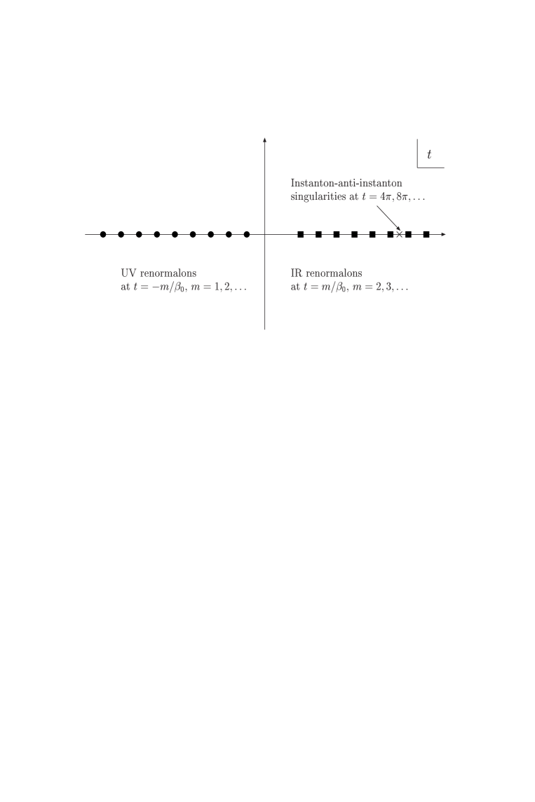
Figure 1: Singularities in the Borel plane of $\Pi(Q^{2})$. The singular points are shown, but not the cuts attached to each of them.

To illustrate these concepts and survey the known singularities, we consider the correlation functions of two vector currents $j_{\mu}=\bar{q}\gamma_{\mu}q$ of massless quarks

$$(-i)\int\,d^{4}x\,e^{-iqx}\,\langle 0|T\,(j_{\mu}(x)j_{\nu}(0))|0\rangle=\left(q_{\mu}q_{\nu}-q^{2}g_{\mu\nu}\right)\,\Pi(Q^{2})$$ (10)

with $Q^{2}=-q^{2}$. The singularities in the Borel plane are shown in Fig. 1. How general is this picture? In QCD, ultraviolet renormalon and instanton-antiinstanton singularities always occur at the locations indicated in the figure, independent of the particular observable, because the physics they represent (ultraviolet behavior and vacuum structure, respectively) is universally the same. The location of IR renormalon singularities depends on the specific observable. For observables derived from off-shell correlation functions, such as $\Pi(Q^{2})$ and the GLS sum rule, IR renormalon singularities occur at integer multiples of $1/\beta_{0}$, because the OPE is an expansion in even powers of the hard scale. For observables derived from on-shell correlation functions, one can have power corrections suppressed by only one power of the hard scale. These would be related to a singularity at $t=1/(2\beta_{0})$. In general, one can construct infrared finite observables, which are arbitrarily infrared-sensitive. $\!{}^{{\bf?}}$ IR renormalons can then occur at any $t$ and arbitrarily close to 0.

2.2 IR Renormalons and the Operator Product Expansion

From Eq. (5) we learned that factorial divergence arises if the typical loop momentum $k\to 0$ as the order of perturbation theory increases. We take this to be the definition of what we mean by “IR renormalon”, i.e. an IR renormalon is a singularity of the Borel transform that is eliminated if all loop momenta are restricted to $k>\Delta$ no matter how small $\Delta$ is. By definition the analysis of IR renormalons is the analysis of small momentum contributions to Feynman amplitudes. This appears complicated since IR renormalons refer to large orders in perturbation theory and so it seems that we would need to investigate the infinite set of Feynman diagrams. We shall now see that the factorization properties of Green functions strongly constrain the form IR renormalon divergence can take. $\!{}^{{\bf?},{\bf?}}$

For the remainder of this subsection we restrict ourselves to observables derived from off-shell (Euclidean) correlation functions; the function $\Pi(Q)$ defined in Eq. (10) will serve as an example. The factorization of small loop momentum regions is done for us by the operator product expansion $\!{}^{{\bf?},{\bf?},{\bf?}}$ (OPE), which for $\Pi(Q)$ reads

$$\Pi(Q)=C_{0}(\alpha_{s},Q/\mu)+\frac{1}{Q^{d}}\,C_{d}(\alpha_{s},Q/\mu)\,\langle\frac{\alpha_{s}}{\pi}G^{2}\rangle(\mu)+O(1/Q^{6}),$$ (11)

where $d=4$ and the leading power correction is given by the gluon condensate. The conventional way of interpreting this formula is to take $C_{0}$ as the series computed with the standard rules of QCD perturbation theory. This includes the small loop momentum regions which give rise to IR renormalons. It is conceptually more satisfactory to include these regions into the definition of the vacuum condensates – the OPE guarantees that this can always be done. The series expansion of $C_{0}$ then differs from the standard one and is free from IR renormalons. Both $C_{0}$ and the vacuum condensates are in this case separately well-defined. In the following we shall adhere to the conventional interpretation, but we will return to the second more appealing one later in this section.

Since any loop momentum region with $k<\Delta$ can be absorbed into a series of vacuum expectation values, the IR renormalon contribution to $C_{0}$ must take the factorized form

$$C_{0}^{\rm IR}(\alpha_{s},Q/\mu)=\frac{1}{Q^{d}}\,C_{d}(\alpha_{s},Q/\mu)\,\mu^{d}M(\alpha_{s})+O(1/Q^{6}),$$ (12)

with the same coefficient function $C_{d}$ as in Eq. (11) and $M(\alpha_{s})$ a (dimensionless) perturbative series independent of $Q$. The coefficient function of the gluon condensate, $C_{d}$, satisfies the renormalization group equation

$$\left(\mu^{2}\frac{\partial}{\partial\mu^{2}}+\beta(\alpha_{s})\frac{\partial}{\partial\alpha_{s}}-\frac{\gamma(\alpha_{s})}{2}\right)C_{d}(\alpha_{s},Q/\mu)=0,$$ (13)

where $\alpha_{s}=\alpha_{s}(\mu)$ and $\gamma(\alpha_{s})$ is the anomalous dimension of the gluon condensate. Since $C_{0}$ and hence $C_{0}^{\rm IR}$ is independent of $\mu$, this implies that

$$\left(\beta(\alpha_{s})\frac{\partial}{\partial\alpha_{s}}+\frac{d+\gamma(\alpha_{s})}{2}\right)M(\alpha_{s})=0.$$ (14)

Here it is used that $M$ being independent of $Q$ and dimensionless cannot depend explicitly on $\mu$. The IR renormalon divergence must be contained entirely in $M$. We make the ansatz

$$M(\alpha_{s})=\sum_{n}\alpha_{s}^{n+1}K(a\beta_{0})^{n}n!\,n^{b}\left(1+\frac{s_{1}}{n}+O(1/n^{2})\right)$$ (15)

and insert it into Eq. (14). We use $\beta(\alpha_{s})=-\beta_{0}\alpha_{s}^{2}-\beta_{1}\alpha_{s}^{3}-\ldots$ and $\gamma(\alpha_{s})=\gamma_{0}\alpha_{s}+\ldots$ and after shifting the summation index $n$ in some terms and expanding in $1/n$, we obtain

$$0 = \sum_{n}\alpha_{s}^{n+1}K(a\beta_{0})^{n}n!\,n^{b}\bigg{[}\frac{d}{2}-\frac{1}{a}$$ (16)

$$\hskip 28.45274pt+\,\frac{1}{n}\bigg{(}\frac{b}{a}-\frac{\beta_{1}}{a^{2}\beta_{0}^{2}}+\frac{\gamma_{0}}{2a\beta_{0}}+\bigg{(}\frac{d}{2}-\frac{1}{a}\bigg{)}s_{1}\bigg{)}+O(1/n^{2})\bigg{]}$$

This implies that either $K=0$, in which case there is no factorial divergence, or otherwise we must have

$$a=\frac{2}{d},\qquad b=\frac{d\beta_{1}}{2\beta_{0}^{2}}-\frac{\gamma_{0}}{2\beta_{0}}.$$ (17)

In the case of the gluon condensate we have $d=4$ and $\gamma_{0}=0$, in which case we reproduce the result originally derived by Mueller $\!{}^{{\bf?}}$ in a different way. Note that $s_{1}$ and higher-order terms are also determined by the $\beta$-function and the anomalous dimension. $\!{}^{{\bf?}}$

It is important to stress the general nature of this result, since it applies to all observables for which we know the structure of power corrections. There may be power corrections and no corresponding IR renormalons, i.e. $K=0$, even if the higher-dimension operator has a power divergence (and hence a perturbative contribution). This can occur in conformal theories such as supersymmetric Yang-Mills theory with four unbroken supersymmetries. However, if the divergence occurs, the $n$-dependence is completely determined by renormalization constants, the perturbative expansion of $C_{d}$ and the truly “non-perturbative” parameter $K$. $\!{}^{{\bf?},{\bf?}}$ There is a common misconception that the involvement of the non-abelian $\beta$-function coefficient $\beta_{0}$ in the location of the renormalon singularity is only a “conjecture”. This misconception is based on the set of fermion bubble diagrams (see the next subsection), which gives only part of $\beta_{0}$. It is indeed difficult to identify diagrammatically the factor $\beta_{0}^{n}$, but the renormalization group allows us to bypass the difficulty. This should not be too surprising since the origin of renormalons is large logarithms. Hence we can prove the factor $\beta_{0}^{n}$, if the renormalon singularity exists, but we cannot rigorously prove that renormalons exist in QCD, for we cannot exclude that $K=0$ for some mysterious (hence entirely improbable) reason.

Suppose we had excluded all loop momenta $k<\Delta$ from the coefficient functions. The IR renormalon would then reappear as the coefficient of an ultraviolet power divergence of the gluon condensate, although the condensate being defined non-perturbatively with the cutoff $k<\Delta$, there is no need to separate this divergence from the remaining condensate. It is however instructive to see how this works in an example. We cannot compute condensates analytically in QCD, but the non-linear $O(N)$ $\sigma$-model in two space-time dimensions provides a nice toy model, $\!{}^{{\bf?},{\bf?},{\bf?},{\bf?},{\bf?},{\bf?}}$ which is solvable in a $1/N$-expansion. As QCD it has only massless particles in perturbation theory, but exhibits dynamical mass generation non-perturbatively and a mass gap in the spectrum. It is asymptotically free, as is QCD, and $m$, the dynamical mass of the $\sigma$-particle, is the analogue of the QCD scale $\Lambda$. We cannot go into the details of the model here except to say that the vacuum expectation value of the square of the auxiliary field $\alpha(x)$,

$$\langle\alpha^{2}\rangle(\mu,m)=\int\limits_{p^{2}<\mu^{2}}\frac{d^{2}p}{(2\pi)^{2}}\,4\pi\sqrt{p^{2}(p^{2}+4m^{2})}\left[\ln\frac{\sqrt{p^{2}+4m^{2}}+\sqrt{p^{2}}}{\sqrt{p^{2}+4m^{2}}-\sqrt{p^{2}}}\right]^{-1}\!,$$ (18)

can be considered as the $\sigma$-model analogue of $\langle\alpha_{s}G^{2}\rangle$. Note that the restriction $p^{2}<\mu^{2}$ defines the otherwise singular operator product $\alpha^{2}$. The integral can be evaluated $\!{}^{{\bf?},{\bf?}}$ with the result

$$\langle\alpha^{2}\rangle(\mu,m)=m^{4}\left[\mbox{Ei}(\ln A)+\mbox{Ei}(-\ln A)-\ln\ln A-\ln(-\ln A)-2\gamma_{E}\right],$$ (19)

where $\gamma_{E}=0.5772\ldots$ is Euler’s constant, $\mbox{Ei}(-x)=-\int_{x}^{\infty}dt\,e^{-t}/t$ the exponential integral function and

$$A=\left(\sqrt{1+\frac{\mu^{2}}{4m^{2}}}+\sqrt{\frac{\mu^{2}}{4m^{2}}}\,\right)^{4}.$$ (20)

Note that $F(x)\equiv\mbox{Ei}(-x)-\ln x$ has an essential singularity at $x=0$ but no discontinuity.

Equation (19) is proportional to the dynamically generated scale to the fourth power, as expected, but for $\mu\gg m$ it develops power-like cutoff dependence. To see the emergence of renormalons, we expand the vacuum expectation value in powers of $m/\mu$ and the $\sigma$-model coupling $\hat{g}(\mu)\equiv-\beta_{0}g(\mu)=1/\ln(\mu^{2}/m^{2})$. To perform the expansion we need the asymptotic expansion of $F(x)$ at large $x$. For positive argument the asymptotic expansion is

$$F(x)=-\ln x+e^{-x}\sum_{n=0}^{\infty}(-1)^{n+1}\,\frac{n!}{x^{n+1}}.$$ (21)

If the divergent series is understood as its Borel sum, the right hand side equals $F$. For negative, real argument, one obtains the asymptotic expansion

$$F(-x)=e^{x}\left[\,\sum_{n=0}^{\infty}\frac{n!}{x^{n+1}}-e^{-x}\left(\ln x\mp i\pi\right)\right].$$ (22)

Note the “ambiguous” imaginary part in the exponentially small term. The interpretation of Eq. (22) is as follows: the upper (lower) sign is to be taken, if the (non-Borel-summable!) divergent series is interpreted as the Borel integral in the upper (lower) complex plane. With this interpretation Eq. (22) is exact and unambiguous. Inserting these expansions, the condensate is given by

$$\langle\alpha^{2}\rangle(\mu,m) = \mu^{4}\sum_{n=0}^{\infty}\left(\frac{\hat{g}(\mu)}{2}\right)^{n+1}\!\!\!\!n!\,+\,2\hat{g}(\mu)\,\mu^{2}m^{2}$$ (23)

$$+\,m^{4}\left[-2\ln\frac{2}{\hat{g}(\mu)}\pm i\pi-2\gamma_{E}-4\hat{g}(\mu)+\frac{\hat{g}(\mu)^{2}}{2}\right]+O\!\left(\frac{m^{6}}{\mu^{2}}\right).$$

The expansion for large $\mu$ has quartic and quadratic terms in $\mu$, parametrically larger than the “natural magnitude” of the condensate of order $m^{4}$. The power terms in $\mu$ arise from the quartic and quadratic divergence of the Feynman integral (18), i.e. from loop momentum $p\sim\mu$. The $\mu$-dependence cancels with the $\mu$-dependence of the coefficient functions in the OPE. In particular the $\mu^{4}$-term cancels with the coefficient function of the unit operator. The important point to note is that the condensate is unambiguous, but separating the “perturbative part” of order $\mu^{4}$ is not, since the asymptotic expansion for $\mu/m\gg 1$ leads to divergent, non-sign-alternating series expansions, which require a summation prescription. The “non-perturbative part” of order $m^{4}$ depends on this prescription (via $\pm i\pi$ in Eq. (23)). In a purely perturbative calculation, one would only obtain the divergent series expansion. The infrared renormalon ambiguity of this expansion would lead us to correctly infer the existence of a non-perturbative power correction of order $m^{4}$. For quantities without an OPE this is one of the main motivations for considering IR renormalon divergence.

The renormalon ambiguity does not allow us in general to say much about the magnitude of the power correction which is determined by other terms, such as $\ln(2/\hat{g})$ in Eq. (23). The $\sigma$-model is somewhat special in this respect, since the power-like ambiguities in defining perturbative expansions are also parametrically smaller in $1/N$ than the actual condensates. This tells us that some caution is necessary in identifying the magnitude of the “renormalon ambiguity” with the magnitude of power corrections. It is probably more appropriate to say that power corrections are expected to be at least as large as perturbative ambiguities. On the other hand, a similar parametric suppression of perturbative ambiguities does not seem to take place in QCD.

2.3 The Large-$\beta_{0}$ Limit

The best representative of renormalon divergence is the set of fermion “bubble diagrams”. Renormalons have originally been discovered $\!{}^{{\bf?},{\bf?},{\bf?}}$ in this set of diagrams. It is important to bear in mind that the concept of renormalons is more general and that all diagrams eventually contribute to the overall constant $K$ that appears for example in Eq. (15). However, the bubble graphs are useful for explicit calculations. With a certain amount of extrapolation they have also turned out to give useful approximations to perturbative expansions in QCD.

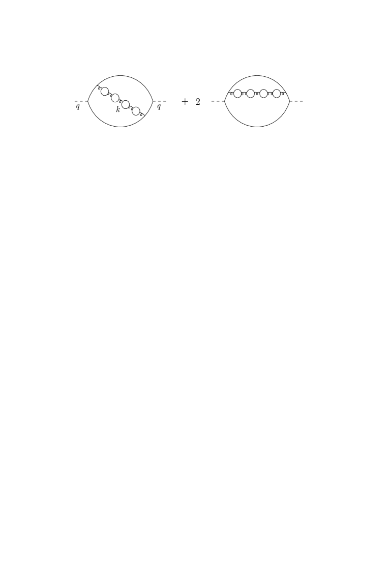
Figure 2: The set of “bubble” diagrams consists of all diagrams with any number of fermion loops inserted into a single gluon line.

We consider again the current correlation function defined in Eq. (10), more precisely the Adler function $D(Q)=4\pi^{2}\,d\Pi(Q)/dQ^{2}$, and compute the “bubble diagrams” shown in Fig. 2. Any number of quark loops may be inserted into the gluon line; each loop gives a factor $\beta_{0f}\alpha_{s}\left[\ln(-k^{2}/\mu^{2})-5/3\right]$, if the strong coupling is renormalized in the $\overline{\rm MS}$ scheme, and $\beta_{0f}=-N_{f}/(6\pi)$ is the quark contribution to the 1-loop $\beta$-function.

Bubble diagrams can be computed in several ways. Originally $\!{}^{{\bf?},{\bf?}}$ the Borel transform was computed directly. The result is $\!{}^{{\bf?}}$

$$B[D](u)=\frac{32}{3\pi}\left(\frac{Q^{2}}{\mu^{2}}e^{-5/3}\right)^{-u}\frac{u}{1-(1-u)^{2}}\,\sum_{k=2}^{\infty}\frac{(-1)^{k}k}{(k^{2}-(1-u)^{2})^{2}}$$ (24)

with $u=\beta_{0f}t$. This has the singularities shown in Fig. 1 except for the presence of $\beta_{0f}$ rather than $\beta_{0}$. The origin of the singularities is more evident, if we integrate over the loop momentum of the “large” quark loop in Fig. 2 and the angles of the gluon momentum $k$. Defining $l=-k^{2}/Q^{2}$, we obtain

$$D=\sum_{n=0}^{\infty}\,\alpha_{s}\int_{0}^{\infty}\,\frac{dl}{l}\,F(l)\,\left[-\beta_{0f}\alpha_{s}\ln\left(l\frac{Q^{2}e^{-5/3}}{\mu^{2}}\right)\right]^{n},$$ (25)

where $\!{}^{{\bf?}}$

$$F(l) \!=\! \frac{8l}{3\pi}\bigg{\{}\bigg{(}{7\over 4}-\ln l\bigg{)}\,l+(1+l)\,\Big{[}\mbox{Li}_{2}(-l)+\ln l\,\ln(1+l)\Big{]}\bigg{\}}\quad l<1,$$

$$F(l) \!=\! \frac{8l}{3\pi}\bigg{\{}1+\ln l+\bigg{(}{3\over 4}+{1\over 2}\,\ln l\bigg{)}\,{1\over l}$$ (26)

$$\qquad\mbox{}+(1+l)\,\Big{[}\mbox{Li}_{2}(-l^{-1})-\ln l\,\ln(1+l^{-1})\Big{]}\bigg{\}}\quad l>1$$

with $\mbox{Li}_{2}(x)$ the dilogarithm. The dominant contributions to the integral come from $l\gg 1$ and $l\ll 1$, because of the large logarithmic enhancements in these regions. There is a one-to-one correspondence between each term in the expansion for small (large) $l$ and the IR (UV) renormalon poles in the Borel transform. For instance, the leading term at small $l$,

$$F(l)=\frac{2}{\pi}\,l^{2}+{\cal O}(l^{3}\ln l)$$ (27)

leads to

$$D^{\rm IR}\sim\frac{1}{\pi}\,\frac{\mu^{4}}{Q^{4}}\,e^{10/3}\sum_{n=0}^{\infty}\alpha_{s}^{n+1}\left(\frac{\beta_{0f}}{2}\right)^{n}n!,$$ (28)

which corresponds to the IR renormalon pole at $u=2$.

We can verify explicitly the general result that this expansion can be interpreted as part of the gluon condensate. When $k\to 0$ the gluon line in Fig. 2 can be “cut”, i.e. supposed to end in a slowly varying external field. The result of the computation is $2\pi/(3Q^{4})$, the leading-order coefficient function of the gluon condensate. To verify that indeed

$$D^{\rm IR}\sim\frac{2\pi}{3Q^{4}}\,\langle\frac{\alpha_{s}}{\pi}G^{2}\rangle(k<\mu),$$ (29)

we compute the (perturbative) gluon condensate in the bubble approximation and obtain $\!{}^{{\bf?},{\bf?}}$

$$\langle\frac{\alpha_{s}}{\pi}G^{2}\rangle(k<\mu) = \frac{3}{2\pi^{3}}\sum_{n=0}^{\mu^{2}}\,\alpha_{s}\int\limits_{0}^{\infty}dk^{2}\,k^{2}\left[-\beta_{0f}\alpha_{s}\ln\left(\frac{k^{2}e^{-5/3}}{\mu^{2}}\right)\right]^{n}$$ (30)

$$=\,\frac{3}{2\pi^{3}}\,\mu^{4}e^{10/3}\sum_{n=0}^{\infty}\alpha_{s}^{n+1}\left(\frac{\beta_{0f}}{2}\right)^{n}n!.$$

Combining this result with the coefficient function, there is agreement with Eq. (28).

The problem with the bubble approximation in QCD is that the renormalon singularities are determined by the quark contribution to the $\beta$-function. The general arguments tell us that $\beta_{0f}$ must get converted into $\beta_{0}$. We could add gluon and ghost bubbles as well, but this would still not give a complete result. In one way or another, recovering $\beta_{0}$ in QCD leads beyond the approximation of a single dressed gluon line. Even if we could construct an effective charge analogous to QED, giving the complete $\beta_{0}$ for every dressed gluon line, it is not clear what would be gained from such a construction, since the overall normalization of renormalon divergence remains as elusive as before, and this constant is all that is not already determined by renormalization group arguments.

Despite these diagrammatic difficulties it has been suggested $\!{}^{{\bf?},{\bf?},{\bf?},{\bf?}}$ to use the quark bubble calculation with $\beta_{0f}$ replaced by $\beta_{0}$ as a realistic approximation to the full QCD perturbative expansion. Formally, this amounts to rewriting a perturbative coefficient at order $\alpha_{s}^{n+1}$ as

$$r_{n}=r_{n0}+r_{n1}N_{f}+\ldots+r_{nn}N_{f}^{n}=r_{0}\left[d_{n}\beta_{0}^{n}+\delta_{n}\right],$$ (31)

where $d_{n}=(-6\pi)^{n}r_{nn}/r_{0}$, $\beta_{0}=(11-2N_{f}/3)/(4\pi)$ and $N_{f}$ is the number of massless quarks. The coefficients $d_{n}$ are then obtained from a calculation of fermion bubble graphs, while the remainder $\delta_{n}$ is neglected. For this reason, this procedure is often referred to as the “large-$\beta_{0}$ approximation”. It can also be viewed as an extension of Brodsky-Lepage-Mackenzie scale setting. $\!{}^{{\bf?}}$ It is more an empirical observation than a well-reasoned statement that the remainder is indeed often found to be small compared to the $\beta_{0}$ term (in the $\overline{\rm MS}$ scheme). Since the large-$\beta_{0}$ limit also incorporates the expected divergence of the QCD expansion, it has turned out to be a useful quantitative tool to estimate higher-order coefficients, in particular when the onset of divergence is rapid and when the observable depends only on a single scale.

2.4 IR Renormalons and Power Corrections in Quantities without an Operator Product Expansion

Up to now we have been characterizing infrared renormalon divergence using known operator product expansion (OPE) methods. Much of the interest in IR renormalons during the recent 5 years comes from adopting a somewhat different point of view. Rather than concentrating on quantities whose OPE is well understood, let us take any “hard” quantity, i.e. a quantity that admits a perturbative calculation. If we are able to identify a particular pattern of IR renormalon divergence, we must replace the IR sensitive perturbative contributions by a non-perturbative parameter of similar magnitude. In this way, the suppression of power corrections can be obtained in a very general way.

To our knowledge this possibility was first mentioned by Mueller, $\!{}^{{\bf?}}$ who suggested to investigate hadronic event shape observables and jet cross sections from this perspective. The idea fell into oblivion at the time and it took another decade before renormalons in observables without an OPE were beginning to be studied in detail, first in heavy quark physics $\!{}^{{\bf?},{\bf?}}$ and soon after for event shape observables. $\!{}^{{\bf?},{\bf?}}$

It is characteristic of off-shell processes that IR renormalons occur only at positive integer multiples of $1/\beta_{0}$, which implies power corrections in powers of $1/Q^{2}$ and not powers of $1/Q$, where $Q$ is the “hard” scale of the process. On-shell quantities have a large variety of infrared-sensitive regions in their Feynman amplitudes and the generic situation leads to IR renormalons at positive half-integers and integers and a series of power corrections in $1/Q$. Due to the variety of possibilities, we restrict ourselves here to a few very general remarks. The most interesting cases are then discussed in detail in Sect. 3.

The existence of $1/Q$ power corrections in observables related to on-shell Green functions can already be seen from the simplest example, the two-point function of a heavy quark field, $\Sigma(p,m)$. The 1-loop contribution is, schematically,

$$\Sigma(p,m)\propto\int\frac{d^{4}k}{(2\pi)^{4}}\frac{N}{k^{2}(2p\cdot k+k^{2}+[p^{2}-m^{2}])}.$$ (32)

Only the denominator is important for the following discussion. Off-shell ($p^{2}\not=m^{2}$) the contribution to the integral from $k<\Lambda$ is of order $C\Lambda^{2}/m^{2}$ relative to the dominant contribution from $k\sim m$. As $p^{2}\to m^{2}$ the coefficient $C$ diverges. Indeed, at $p^{2}=m^{2}$ the integrand of Eq. (32) vanishes only linearly with $k$ for small $k$; hence we expect a non-perturbative contribution to $\Sigma(m,m)$ of relative order $\Lambda/m$.

Similar power counting arguments apply to hadronic event shape observables. The basic parton emission processes in QCD are infrared divergent for soft and collinear emissions. Event shape observables are constructed to suppress these soft and collinear contributions, so that they are infrared finite in perturbation theory. But the residual contribution from small momentum regions is usually suppressed only by a single power of the hard scale. In general high-energy processes involving massless quarks the infrared contributions can be classified as soft or hard-collinear. It appears, however, that power corrections from hard-collinear regions (energy $\omega$ much larger than transverse momentum $k_{\perp}$) are always suppressed by powers of $Q^{2}$ rather than $Q$. We do not know of a proof of this statement, but the following heuristic argument may illustrate the point: let $p$ be the momentum of a fast on-shell particle, $p\sim Q$, after emission of a hard-collinear on-shell particle with $\omega\sim Q$, $k_{\perp}\ll Q$, where $k_{\perp}$ is the transverse momentum relative to $p$. Then the propagator

$$\frac{1}{(p+k)^{2}}=\frac{1}{p\left(\omega-\sqrt{\omega^{2}+k_{\perp}^{2}}\right)}$$ (33)

is expanded in $k_{\perp}^{2}/\omega^{2}\sim k_{\perp}^{2}/Q^{2}$ and $Q$ enters only quadratically. Since the same is true of the hard-collinear phase space, it may be argued that the transverse momentum, and hence $Q$, always enters quadratically as long as energies are large. As a consequence, if $1/Q$ power corrections exist and if one is interested only in those, the analysis simplifies, because only soft contributions need to be considered.

A systematic analysis of IR renormalons for general short-distance processes has therefore much in common with the analysis of IR finiteness with the methods of perturbative factorization. It extends the notion of IR safety (absence of logarithmic divergences) to that of IR sensitivity (power-suppressed IR contributions). From a very general point of view, the most important lesson drawn from IR renormalons is the existence of a correlation between the size of non-perturbative corrections and the size of perturbative coefficients in large orders, often already at 2 loops.

2.5 The Landau Pole

In closing this overview section we address a common misunderstanding that the existence of renormalons and summation ambiguities is related to an infrared Landau pole in the running coupling. A consequence of this misunderstanding is that it is often thought that the power corrections identified via IR renormalons have something to do with the definition of the QCD coupling. It is true that the factorial divergence follows from the fact that the coupling evolves ($\beta_{0}\not=0$). The power correction indicated by this divergence is, however, a property of the particular observable and it would exist even if the coupling did not evolve.

To see how the association with the Landau pole might arise, we interchange the summation and integration in Eq. (25). The interchange is mathematically not legitimate, but if we nonetheless proceed, we obtain

$$D=\int_{0}^{\infty}\,\frac{dl}{l}\,F(l)\,\alpha_{s}\!\left(ke^{-5/6}\right),$$ (34)

where $k^{2}=-lQ^{2}$ and

$$\alpha_{s}(k)=\frac{\alpha_{s}(\mu)}{1+\alpha_{s}(\mu)\beta_{0}\ln(k^{2}/\mu^{2})}\equiv\frac{1}{\beta_{0}\ln k^{2}/\Lambda^{2}}$$ (35)

is the 1-loop running coupling. The Landau pole of the coupling lies on the $l$-integration contour and the ambiguity in defining the integral (34) due to this Landau pole is exactly identical to the ambiguity in defining the Borel integral of the divergent series expansion.

This apparent connection does not persist beyond the calculation of bubble diagrams. The reason is that in the same approximation in which we keep only the bubble diagrams, the $\beta$-function can only have a single term: $\beta(\alpha_{s})=-\beta_{0}\alpha_{s}^{2}$. The existence of a Landau pole is then an automatic consequence. The general theory of renormalons shows that the leading asymptotic behavior depends only on $\beta_{0}$ and $\beta_{1}$, see Eqs. (15,17). On the other hand whether a Landau pole exists or not is a strong-coupling problem and it depends on all coefficients of the $\beta$-function, and on power corrections to the running of the coupling. This can be studied explicitly for $\beta$-functions with only two independent terms. $\!{}^{{\bf?},{\bf?},{\bf?}}$ For example, the integral (34) might be well-defined, but its series expansion remains still divergent. It would then be incorrect to conclude that the power corrections indicated by IR renormalons are properly taken into account by summing the series to the numerical value given by the integral. Such a summation prescription would be related to a certain definition of non-perturbative parameters relevant to the particular process, but it would not render these parameters zero and superfluous. In essence, IR renormalons reflect perturbative aspects of non-perturbative corrections (namely their power divergences) for a specific observable, whereas the existence of a Landau pole is a wholly non-perturbative issue, but not related to any particular observable. This can again be non-perturbatively verified in the non-linear $O(N)$ $\sigma$-model, $\!{}^{{\bf?}}$ where the propagator of the $\alpha$-field defines an effective coupling without Landau pole, but all correlation functions contain the full series of IR renormalon poles.

3 Applications

3.1 Deep Inelastic Scattering

We begin with a short exposition of the applications of renormalons to the structure functions of deep inelastic scattering. Since the operator product expansion is available, this example serves to illustrate the operator interpretation of renormalons and formulate phenomenological procedures that can be generalized to other, more complicated situations.

The GLS Sum Rule

The GLS sum rule, defined in Eq. (1), has already been discussed in the introduction; here we complete this discussion.

The first IR renormalon singularity at $t=1/\beta_{0}$ corresponds to a single twist-4 operator $\!{}^{{\bf?}}$ and can be obtained with the methods described in Sect. 2. Combining this result with the calculation of the leading ultraviolet renormalon $\!{}^{{\bf?}}$ (see Sect. 4), we find the large-order behavior

$$r_{n}\sim\beta_{0}^{n}\,n!\,\Big{[}K^{\rm UV}\,(-1)^{n}n^{1-\beta_{1}/\beta_{0}^{2}+\lambda_{1}}+\,K^{\rm IR}\,n^{\beta_{1}/\beta_{0}^{2}-32b/9}\Big{]},$$ (36)

where $r_{n}$ is the coefficient of $\alpha_{s}^{n+1}$, $\beta_{0,1}$ are the first two coefficients of the $\beta$-function, $b=4\pi\beta_{0}=11-2N_{f}/3$ and $\lambda_{1}$ is related to the anomalous dimension matrix of four-fermion operators, see Sect. 4. For $N_{f}>2$, the UV renormalon behavior dominates the asymptotic behavior at very large $n$ because of its larger power of $n$. However, the overall normalization constants $K^{\rm UV}$ and $K^{\rm IR}$ are not known. Since the $\overline{\rm MS}$ scheme favors large residues of IR renormalons, at least in the large-$\beta_{0}$ approximation, we expect fixed-sign IR renormalon behavior in intermediate orders. The first three terms in the series known exactly are indeed of the same sign in the $\overline{\rm MS}$ scheme as can be seen from Eq. (1).

Is the asymptotic behavior in Eq. (36) relevant to phenomenology? Since the constants $K$ are not known, we consider $\!{}^{{\bf?},{\bf?}}$ the large-$\beta_{0}$ approximation. The Borel transform (defined by Eq. (7)) of the perturbative expansion in this approximation is given by $\!{}^{{\bf?}}$

$$B[1-I_{\rm GLS}/3](u)=\left(\frac{Q^{2}}{\mu^{2}}\,e^{C}\right)^{-u}\,\frac{1}{9\pi}\left\{\frac{8}{1\!-\!u}+\frac{4}{1\!+\!u}-\frac{5}{2\!-\!u}-\frac{1}{2\!+\!u}\right\},$$ (37)

where $u=\beta_{0}t$. This is much simpler than what we would have expected on general grounds. In particular, there are only four renormalon poles, all others being suppressed in the large-$\beta_{0}$ limit. The structure of the leading singularities is also simpler than the exact result in Eq. (36), because the anomalous dimensions should be set to zero in this limit. Nonetheless, the exact $r_{1},r_{2}$ are reproduced reasonably well by the large-$\beta_{0}$ limit. The large-$\beta_{0}$ approximation taken at face value implies that the minimal term of the series is reached at order $\alpha_{s}^{3}$ or $\alpha_{s}^{4}$ at $Q^{2}=3\,$GeV², a momentum transfer relevant to the CCFR experiment. Hence it is not clear whether at $Q^{2}=3\,$GeV² the perturbative prediction could be improved further by exact calculations of higher-order corrections. Further improvement would then require the inclusion of twist-4 contributions, and in particular a practically realizable procedure to combine them consistently with the perturbative series. This hypothesis is further supported by noting that the integral over loop momentum is dominated by $k\sim 450\,$MeV at order $\alpha_{s}^{3}$ and $k\sim 330\,$MeV at order $\alpha_{s}^{4}$. The ambiguity in summing the perturbative expansion is of order (assuming $\Lambda_{\overline{\rm MS}}=215\,$MeV)

$$\frac{1}{3}\,\delta I_{\rm GLS}=\frac{1}{\beta_{0}}\frac{8e^{5/3}}{9\pi}\,\frac{\Lambda^{2}_{\overline{\rm MS}}}{Q^{2}}\approx\frac{0.1\,\mbox{GeV}^{2}}{Q^{2}}.$$ (38)

This should be compared to the twist-4 contribution to the same quantity estimated in quark model and by QCD sum rules $\!{}^{{\bf?}}$

$$-\frac{8}{27}\,\frac{\langle\langle{\cal O}_{4}\rangle\rangle}{Q^{2}}\approx-\frac{0.1\,\mbox{GeV}^{2}}{Q^{2}},$$ (39)

where $\langle\langle{\cal O}_{4}\rangle\rangle$ is the reduced nucleon matrix element of the twist-4 operator. The two are comparable, which suggests that the treatment of perturbative corrections beyond those known exactly is as important for a determination of $\alpha_{s}$ from the GLS sum rule as the twist-4 correction.

The $x$-Dependence of Power Corrections to Structure Functions

The operator product expansion allows us to express $1/Q^{2}$ corrections to the structure functions in terms of contributions of several towers of twist-4 operators $\!{}^{{\bf?}}$ or, equivalently, several multiparton correlation functions. $\!{}^{{\bf?},{\bf?},{\bf?}}$ Unfortunately, the structure of the corrections is complicated and they involve many non-perturbative parameters which cannot all be extracted from inclusive measurements. Because of this, it has never been possible to use this sophisticated machinery in the analysis of real data. In practice, higher-twist corrections are being extracted from data from a combined fit to perturbative and $1/Q^{2}$-suppressed contributions in a large $Q^{2}$ range.

Renormalons provide a simple ansatz for the $x$-dependence of power corrections involving fewer (if any) non-perturbative parameters. As in most other applications divergences of the perturbative series are relevant inasmuch as they originate from small momentum regions in Feynman diagrams that are also responsible for non-perturbative effects. To explain the idea, recall that the structure functions (take $F_{2}(x)$ as an example) are related to the parton distribution functions $P(x)$, $P=q,\bar{q},g$ through a perturbative expansion and convolution of the form

$$F_{2}(x,Q^{2}) = 2x\sum_{P}\left[e^{2}_{P}+\sum_{n=0}r_{P,n}(x)\alpha_{s}^{n+1}-c_{P}(x)\frac{\mu^{2}}{Q^{2}}\right]\star P(x,Q^{2})$$ (40)

$${}+\frac{C_{2}(x)}{Q^{2}},$$

where $e_{P}$ are the electromagnetic charges of partons and $\star$ stands for the convolution. In this expression we have subtracted contributions of small momenta $k<\mu\ll Q$ from the coefficient functions and defined the higher-twist contribution which can have a complicated operator content as the full contribution (perturbative and non-perturbative) coming from small momenta $k<\mu$. Since twist-4 operators are quadratically divergent, we know that $C_{2}(x)=c^{\prime}(x)\mu^{2}+O(\Lambda^{2})$ if $\mu\gg\Lambda$ and $c^{\prime}(x)=\sum_{P}c_{P}(x)\star P(x)$ so that the dependence on the cutoff $\mu$ cancels.

As $c(x)$ is defined as the small-momentum contribution to Feynman diagrams, it has itself a (divergent) perturbative expansion in $\alpha_{s}$. We then extract the $c(x)$ from the $x$-dependence of the IR renormalon pole computed in the large-$\beta_{0}$ approximation. In this approximation there is only a (anti-)quark contribution and the result is $\!{}^{{\bf?},{\bf?},{\bf?},{\bf?}}$

$$c_{q}^{(L)}(x) = 8x^{2}-4\delta(1-x),$$ (41)

$$c_{q}^{(2)}(x) = -\frac{4}{[1-x]_{+}}+4+2x+12x^{2}-9\delta(1-x)-\delta^{\prime}(1-x),$$ (42)

$$c_{q}^{(3)}(x) = -\frac{4}{[1-x]_{+}}+4+2x+4x^{2}-5\delta(1-x)-\delta^{\prime}(1-x)$$ (43)

for $F_{L}$, $F_{2}$ and $F_{3}$, respectively. A common overall normalization is omitted here, because it plays no role in the following. The ‘+’ prescription is defined as usual by $\int_{0}^{1}dx\,[f(x)]_{+}t(x)=\int_{0}^{1}dx\,f(x)\,(t(x)-t(1))$ for test functions $t(x)$.

If we assume that the subtraction term in the square brackets of Eq. (40) cancels approximately the higher-order perturbative terms, and if we assume that $C_{2}(x)$ is approximated by $c^{\prime}(x)\mu^{2}$, we obtain an improved prediction for the structure functions compared to the fixed-order perturbative approximation. This suggestion, though sometimes motivated by different arguments, has become known as “renormalon model” of power corrections. $\!{}^{{\bf?},{\bf?}}$ The structure functions are then written as

$$F(x,Q)=F^{\rm tw-2}(x,Q)\left(1+\frac{D(x,Q)}{Q^{2}}+O(1/Q^{4})\right),$$ (44)

where $F^{\rm tw-2}(x,Q)$ is the leading-twist result for the structure function $F=F_{L},F_{2},F_{3},\ldots$ and

$$D(x,Q)=\frac{\Lambda^{2}}{F^{\rm tw-2}(x,Q)}\int_{x}^{1}\frac{d\xi}{\xi}\,c(\xi)\,q(x/\xi,\mu)\,$$ (45)

is the model parametrization of the (relative) twist-4 correction. Here $q(x,\mu)$ is the standard (leading-twist) quark density, and $\Lambda$ is a certain scale of order $\Lambda_{\rm QCD}$ which provides the overall normalization. The expression can be extended to include gluon contributions and/or higher-order corrections should they become available.

The overall normalization has been treated differently in the literature. One suggestion has been $\!{}^{{\bf?}}$ to parametrize the normalization of all $1/Q^{2}$ power corrections by a single process-independent number, to be extracted from the data once and related to a a certain effective QCD coupling. Other authors $\!{}^{{\bf?},{\bf?},{\bf?}}$ prefer to adjust the normalization in a process-dependent way and to take only the shape of the $x$-distribution as a prediction of the model. Because of difficulties in constructing the gluon contribution in the model, one may also think of adjusting the normalization of quark and gluon contributions separately.

Figure 3: Relative twist-4 contribution $D(x)$ (called $C_{p,d}(x)$ here) defined by Eq. (45) to the proton (deuteron) structure function $F_{2}$ in the “renormalon model” $\!{}^{{\bf?}}$ (dashed line) compared with proton (filled circles) and deuteron (empty circles) data. $\!{}^{{\bf?}}$ The solid curve shows the unrescaled estimate of the renormalon ambiguity.

The “renormalon model” of twist-4 corrections has first been applied to the structure function $F_{2}$. $\!{}^{{\bf?},{\bf?},{\bf?}}$ As shown in Fig. 3, the shape of the twist-4 correction calculated from the model indeed reproduces the experimental data very well. These results refer to the the non-singlet contribution to $F_{2}$, which is expected to dominate except for small values of $x$. Similar predictions have been worked out for the longitudinal structure function $F_{L}$, $\!{}^{{\bf?},{\bf?}}$ $F_{3}$, $\!{}^{{\bf?},{\bf?}}$ and the polarized structure function $g_{1}$ etc. $\!{}^{{\bf?},{\bf?}}$ More recently a renormalon model prediction has also been constructed for the singlet contribution $\!{}^{{\bf?},{\bf?}}$ to $F_{2}$, which modifies the analysis at small $x$, below those $x$ for which comparison with present data is possible. (The treatment of singlet contributions is more difficult and ambiguous in the renormalon model than non-singlet contributions. The calculation relies on singlet quark contributions, which are then reinterpreted as gluon contributions. $\!{}^{{\bf?}}$)

Figure 4: Twist-4 correction to $xF_{3}$ as extracted from the (revised) CCFR data. The three plots show the effect of including leading order (LO), next-to-leading order (NLO) and next-to-next-to-leading order (NNLO) QCD corrections in the twist-2 term. The data points $\!{}^{{\bf?}}$ are overlaid with the shape obtained from the “renormalon model” for the $1/Q^{2}$ power correction.

A striking property of the renormalon model for twist-4 corrections is that all target-dependence enters trivially through the target dependence of the twist-2 distribution functions. Therefore the renormalon model can be useful only if the genuine twist-4 target dependence is small compared to the magnitude of the twist-4 correction itself. In terms of moments $M_{n}$, Eq. (45) implies

$$\frac{M_{n}^{\rm tw-4}}{M_{n}^{\rm tw-2}}_{|\rm hadron1}=\,\,\,\frac{M_{n}^{\rm tw-4}}{M_{n}^{\rm tw-2}}_{|\rm hadron2}\,.$$ (46)

Figure 3 shows that this is indeed the case for $F_{2}$ of protons against deuterons, in particular in the region of large $x$. More recent analyses $\!{}^{{\bf?},{\bf?}}$ also confirm this fact.

It is known that higher-twist corrections (as well as higher-order perturbative corrections) are enhanced as $x\to 1$. $\!{}^{{\bf?}}$ This is in part an effect of kinematic restrictions near the exclusive region and the renormalon model reproduces such enhancements. For the structure functions it is found that power corrections related to renormalons are of order

$$\left[\frac{\Lambda^{2}}{Q^{2}(1-x)}\right]^{\!n},$$ (47)

at least those related to diagrams with a single gluon line. $\!{}^{{\bf?}}$ This tells us that the increase of the twist-4 correction towards larger $x$ seen in the model and the data in Fig. 3 may to a large extent be the correct parametrization of such a kinematic effect. Note that Eq. (47) can be understood from the fact that the hard scale in DIS is $Q\sqrt{1-x}$ at large (but not too large) $x$.

It is also possible that both the experimental parametrization of higher-twist corrections and the model provide effectively a parametrization of higher-order perturbative corrections to twist-2 coefficient functions. As far as data are concerned, it should be kept in mind that it is obtained from subtracting from the measurement a twist-2 contribution obtained from a truncated perturbative expansion. As far as the renormalon model is concerned, it is best justified by the “ultraviolet dominance hypothesis”. $\!{}^{{\bf?}}$ Since UV contributions to twist-4 contributions can also be interpreted as contributions to twist-2 coefficient functions, a “perturbative” interpretation of the model prediction suggests itself as we have already indicated in the discussion of Eq. (40). Note that higher-order corrections in $\alpha_{s}(Q)$ vary more rapidly with $Q$ than lower order ones, and may not be easily distinguished from a $1/Q^{2}$ behavior, if the $Q^{2}$-coverage of the data is not very large. An interesting hint in this direction is provided by the analysis $\!{}^{{\bf?},{\bf?},{\bf?}}$ of CCFR data on $F_{3}$, reproduced in Fig. 4. The figure shows how the experimentally fitted twist-4 correction gradually disappears as NLO and NNLO perturbative corrections to the twist-2 coefficient functions are included. At the same time, the renormalon model for the twist-4 corrections reproduces well the shape of data at leading order, and hence parametrizes successfully the effect of NLO and (approximate) NNLO corrections. This is an important piece of information, relevant to quantities for which an NNLO or even NLO analysis is not yet available.

Note that whether the model is interpreted as a model for twist-4 corrections or higher-order perturbative corrections is insignificant inasmuch as renormalons are precisely related to the fact that the two cannot be separated unambiguously. The model clearly cannot be expected to reproduce fine structures of twist-4 corrections. Its appeal draws from the fact that it provides a simple way to incorporate some contributions beyond LO or NLO in perturbation theory, which may be the dominant source of discrepancy with data with the presently achievable accuracy.

3.2 Hadronic Event Shape Variables

The structure of hadronic final states in $e^{+}e^{-}$ annihilation and deep inelastic scattering is the subject of intensive ongoing studies. $\!{}^{{\bf?}}$ This structure is characterized by a set of infrared and collinear safe event shape variables that are calculated in perturbative QCD in terms of quark and gluon momenta and compared to the measured hadron distributions. Apart from a correction for detector effects, the comparison of theory and data therefore requires a correction for hadronization effects that are most commonly modeled using Monte Carlo event generators. It has been known for quite some time $\!{}^{{\bf?}}$ that the hadronization corrections are substantial. In this section we review recent developments that relate hadronization corrections to power corrections of order $\Lambda/Q$ (where $Q$ is the center-of-mass energy in $e^{+}e^{-}$ annihilation) indicated by renormalons in the perturbative prediction for the event shape variables. This connection was suggested $\!{}^{{\bf?},{\bf?}}$ and worked out for a few cases of practical interest $\!{}^{{\bf?}}$ several years ago. These studies provided the first theoretical indications that hadronization corrections to most of the observables should scale as $\Lambda/Q$, i.e. are suppressed by only a single power of the large momentum. Subsequent analyses $\!{}^{{\bf?},{\bf?},{\bf?},{\bf?}}$ confirmed this conclusion.

Most of the discussion below assumes a generic event shape observable $S$ that is of order $\alpha_{s}(Q)$ at leading order. One example is $S=1-T$ where “thrust” $T$ is defined as

$$T=\max_{\,\vec{n}}\frac{\sum_{i}|\vec{p}_{i}\cdot\vec{n}\,|}{\sum_{i}|\vec{p}_{i}|},$$ (48)

where the sum is over all hadrons (partons) in the event. The thrust axis $\vec{n}_{T}$ is the direction at which the maximum is attained. Other event shapes considered in connection with power corrections are the heavy jet mass, jet broadening, C-parameter and the longitudinal cross section in $e^{+}e^{-}$ annihilation, to give only a few examples.

Mean Values of Event Shape Variables

It is relatively easy to understand that event shape observables in $e^{+}e^{-}$ annihilation are linearly sensitive to small parton momenta and hence are expected to receive non-perturbative contributions of order $\Lambda/Q$. Consider an event shape variable that is zero at tree level and therefore related to the matrix element for gluon emission $\gamma^{*}\to q\bar{q}g$ to leading order

$$\langle S\rangle=\int\!\mbox{dPS}[p_{i}]\,|{\cal M}_{q\bar{q}g}|^{2}\,S(p_{i}).$$ (49)

It can be argued that the $\Lambda/Q$ sensitivity arises neither from emission of collinear and energetic partons, nor from soft quarks, but only from soft gluons. Introducing the energy fractions $x_{i}=2p_{i}\cdot q/q^{2}$, and reserving $x_{3}$ for the gluon energy fraction, this implies that the only relevant integration region is $x_{3}\to 0$ and, therefore, the gluon emission can be calculated in the “soft” approximation:

$$|{\cal M}_{q\bar{q}g}|^{2}=32g_{s}^{2}\,\frac{2}{(1-x_{1})\,(1-x_{2})}.$$ (50)

The phase space is, on the other hand

$$\int\!\mbox{dPS}[p_{i}]=\int_{0}^{1}dx_{1}dx_{2}\,\theta(x_{1}+x_{2}-1)\,$$ (51)

and since the matrix element in Eq. (50) is singular as $x_{1,2}\to 1$, there is a potential logarithmic singularity. To obtain an IR finite result, the event shape variable has to be constructed so as to eliminate this divergence. The generic situation with event shapes is a linear suppression of soft gluons, $S(x_{i})\propto x_{3}$ as $x_{3}\to 0$, e.g. for the thrust $1-T=1-{\rm max}(x_{1},x_{2})$ with $x_{1}+x_{2}+x_{3}=2$. It is easy to see that this property implies a contribution of order $\mu/Q$ to the integral in Eq. (49) from gluons with energy less than $\mu$, unless there is some cancelation.

It has been suggested $\!{}^{{\bf?},{\bf?},{\bf?}}$ that the leading power correction to average event shape observables may be described by a single (“universal”) parameter multiplied by an observable-dependent, but calculable, coefficient. Write

$$\langle S\rangle=A_{S}\alpha_{s}(\mu)+\left[B_{S}+A_{S}\beta_{0}\ln\frac{\mu^{2}}{Q^{2}}\right]\alpha_{s}(\mu)^{2}+\ldots+\frac{K_{S}(\mu)}{Q}+O(1/Q^{2}).$$ (52)

Dokshitzer and Webber $\!{}^{{\bf?}}$ parametrize the coefficient of the power correction in the form

$$K_{S}(\mu)=\frac{16c_{S}}{3\pi}\mu_{I}\left[\bar{\alpha}_{0}(\mu_{I})-\alpha_{s}(\mu)-\left(\beta_{0}\ln\frac{\mu^{2}}{\mu_{I}^{2}}+\frac{K}{2\pi}+2\beta_{0}\right)\alpha_{s}(\mu)^{2}\right],$$ (53)

where $\mu_{I}$ is an IR subtraction scale (typically chosen to be $2\,$GeV), $\bar{\alpha}_{0}(\mu_{I})$ is the non-perturbative parameter to be fitted and $K=67/6-\pi^{2}/2-5N_{f}/9$. The remaining terms approximately subtract the IR contributions contained in the perturbative coefficients $A$ and $B$ up to second order. The universality assumption can be tested by fitting the value of $\bar{\alpha}_{0}(\mu_{I})$ or, equivalently, $K_{S}(\mu)/c_{S}$ to different event shape variables.

Figure 5: Energy dependence of $\langle 1-T\rangle$ (upper panel) and the heavy jet mass $\langle M_{H}^{2}/Q^{2}\rangle$ (lower panel) plotted as function of $1/Q$. $\!{}^{{\bf?}}$ Dotted line: second-order perturbation theory with scale $\mu=Q$. Solid line: second-order perturbation theory with power correction added according to Eq. (53) and with $\mu=Q$, $\mu_{I}=2\,$GeV. For $\bar{\alpha}_{0}(2\,\mbox{GeV})$ the fit values 0.543 for thrust and 0.457 for the heavy jet mass $\!{}^{{\bf?}}$ are taken. (Note that this reference uses $c_{1-T}=c_{M_{H}^{2}/s}=1$.) The dashed line shows second order perturbation theory at the very low scale $0.07Q$ with no power correction added. For both observables $\alpha_{s}(M_{Z})$ has been fixed to 0.12.

In Fig. 5 we compare the energy dependence of $\langle 1-T\rangle$ and the heavy jet mass $\langle M_{H}^{2}/Q^{2}\rangle$ with the prediction with and without a $1/Q$ power correction. It is clearly seen that (a) the second-order perturbative result with scale $\mu=Q$ is far too small and (b) the difference with the data points is fitted well by a $1/Q$ power correction.

In absolute terms the power correction added to thrust and the heavy jet mass is about $1\,\mbox{GeV}/Q$. This is a sizeable correction of order $20\%$ even at the scale $M_{Z}$, because the perturbative contribution is of order $\alpha_{s}(M_{Z})/\pi$. The fit for $\bar{\alpha}_{0}$ is sensitive to the choice of renormalization scale $\mu$ and in general to the treatment of higher-order perturbative corrections. There is nothing wrong with this, because the very spirit of the renormalon approach is that perturbative corrections and non-perturbative hadronization corrections are to some extent inseparable. Hence we find it plausible that the $1/Q$ power correction accounts in part for large higher-order perturbative corrections, which are large precisely because they receive large contributions from IR regions of parton momenta. It has been noted $\!{}^{{\bf?}}$ that choosing a small scale, $\mu=0.13Q$, reduces the second order perturbative contribution and power correction significantly for $\langle 1-T\rangle$. In Fig. 5 (dashed curve) we have taken a very low scale, $\mu=0.07Q$, to illustrate the fact that the running of the coupling at this low scale can fake a $1/Q$ correction rather precisely (a straight line in the figure). Note that an analysis of $\langle 1-T\rangle$ in the effective-charge scheme $\!{}^{{\bf?}}$ selects almost the same scale $\mu=0.08Q$. A simultaneous fit $\!{}^{{\bf?}}$ of $\alpha_{s}$, a third-order perturbative coefficient and a $1/Q$ power correction then leads to reduced power correction of order $(0.3\pm 0.1)\,\mbox{GeV}/Q$ consistent with the above argument.

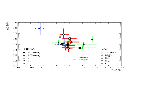
Figure 6: Fit results of $\bar{\alpha}_{0}$ and $\alpha_{S}(M_{\mathrm{Z}})$. $\!{}^{{\bf?}}$

A comprehensive compilation $\!{}^{{\bf?}}$ of the combined fits of the the parameter $\bar{\alpha}_{0}(\mu_{I})$ and the strong coupling $\alpha_{S}(M_{\mathrm{Z}})$ to the data on several event shapes in $e^{+}e^{-}$-annihilation and deep inelastic scattering is shown in Fig. 6. The extracted values of $\bar{\alpha}_{0}$ center around $\bar{\alpha}_{0}(2$ GeV$)\sim 0.5$ that gives some support to the universality hypothesis. Its theoretical status has not been completely elucidated so far, different and somewhat conflicting arguments have been given. $\!{}^{{\bf?},{\bf?},{\bf?}}$ In order to get further insight, a detailed analysis of IR sensitive contributions to the matrix elements for the emission of two partons $\!{}^{{\bf?},{\bf?}}$ has been undertaken. It was found that for $\langle 1-T\rangle$, the jet masses, and the $C$-parameter the coefficient of the $1/Q$ power correction that is obtained for one gluon emission is rescaled by the same factor, often called the “Milan factor”, whose value was later revised to 1.49. $\!{}^{{\bf?},{\bf?}}$ The universality of the Milan factor for a class of event shapes is a direct consequence of the assumed dominance of soft-gluon radiation coupled with an underlying geometrical universality (linearity in transverse momenta of emitted gluons) in the shape variables themselves. $\!{}^{{\bf?}}$ Note that the numerical value of the “Milan factor” is actually not important, since it is likely to be modified by yet higher-order corrections. The universality of the “Milan factor” is hence the more important observation, since it allows us to relate different observables. Nevertheless, the analysis of soft-gluon effects at the 2-loop order is very interesting, since it is represents one of the few cases where power corrections have been explicitly investigated beyond one-gluon exchange for observables that do not have an operator product expansion.

Event Shape Distributions

The structure of power corrections to event shape distributions $(1/\sigma_{tot})d\sigma/dS$ is more complex. (The distributions are defined so that the mean value is given by $\langle S\rangle=(1/\sigma_{tot})\int_{0}^{S_{max}}\!\!dS\,S\,d\sigma/dS$.) In the following we consider event shapes defined so that $S\to 0$ corresponds to the two-jet limit. For small values of the event shape variable $S$ the dynamics of soft-gluon emission depends on two different IR scales $QS$ and $\sqrt{Q^{2}S}$, and $1/Q\ll 1/Q\sqrt{S}\ll 1/(QS)$. The smallest scale of order $QS$ is related to the typical energy carried by soft gluons, while the scale $Q\sqrt{S}$ defines the transverse momenta of the jets, $k_{T}^{2}\sim Q^{2}S$. By examining the sensitivity of perturbative emission of soft gluons with energy of order $QS$ and collinear particles with transverse momentum of order $Q^{2}S$, we are lead to suspect non-perturbative corrections suppressed by powers of both scales. Then, since in the end-point region $S\sim\Lambda/Q$, we can expand the distributions in powers of the larger scale $Q^{2}S$ and keep the leading term only that corresponds to the resummation of all corrections of order $(1/QS)^{k}$, neglecting corrections of order $(1/Q\sqrt{S})^{k}$. The resummation introduces the important concept of a shape function for soft-gluon emission, $\!{}^{{\bf?},{\bf?}}$ which we shall review briefly on the particular example of the thrust distribution $t\equiv 1-T$. $\!{}^{{\bf?}}$

The starting point is the observation that the differential thrust distribution $d\sigma/dt$ in the small $t$ region computed by resumming an infinite number of soft-gluon emissions is expected to exponentiate under a Laplace transformation

$$\frac{1}{\sigma_{tot}}\int_{0}^{t_{\rm max}}\!dt\,e^{-\nu t}\,\frac{d\sigma}{dt}=e^{-S(\nu,Q)}$$ (54)

with the exponent $S(\nu,Q)$ of the general form

$$S(\nu,Q) = \int_{0}^{1}\frac{dx}{x}\left(1-e^{-\nu x}\right)$$ (55)

$$\times\left(\int_{x^{2}Q^{2}}^{xQ^{2}}\!\!\frac{dk_{\perp}^{2}}{k_{\perp}^{2}}\Gamma[\alpha_{s}(k_{\perp}^{2})]+B[\alpha_{s}(xQ^{2})]+C[\alpha_{s}(x^{2}Q^{2})]\right).$$

Here $\Gamma[\alpha_{s}]$ is the universal cusp anomalous dimension that controls soft and collinear gluon emission. (Compared to the original discussion $\!{}^{{\bf?}}$ we have added the additional function $C[\alpha_{s}(x^{2}Q^{2})]$ to the exponent. This function does not appear to the next-to-leading logarithmic accuracy, but we are not aware of a theoretical argument that would not allow terms of this structure in higher-orders. The following discussion proceeds under the assumption that $C[\alpha_{s}(x^{2}Q^{2})]$ does not have a divergent perturbative expansion, as it can happen in Drell-Yan production. $\!{}^{{\bf?}}$) The next step separates the contribution of soft gluons introducing a cutoff in transverse momentum $k_{\perp}<\mu$. Heuristically, the contribution of gluons with $k_{\perp}>\mu$ has to be defined as a perturbative contribution $S_{PT}(\nu,Q,\mu)$ to $S(\nu,Q)$, and contributions of $k_{\perp}<\mu$ have to be promoted to the non-perturbative correction, $S_{NP}(\nu,Q,\mu)$, so that $S(\nu,Q)=S_{PT}(\nu,Q,\mu)+S_{NP}(\nu,Q,\mu)$. From the $\Gamma$-term in Eq. (55), expanding formally in powers of $\nu/Q$ and neglecting all powers of $\nu/Q^{2}$, we obtain $\!{}^{{\bf?}}$

$$S_{NP}(\nu,Q,\mu)\sim\sum_{n>0}\frac{1}{nn!}\left(\frac{-\nu}{Q}\right)^{n}\int\limits_{0}^{\mu^{2}}\!dk_{\perp}^{2}\,k_{\perp}^{n-2}\Gamma[\alpha_{s}(k_{\perp}^{2})].$$ (56)

The integrals over the cusp anomalous dimension should eventually be substituted by (dimensionful) non-perturbative parameters. Since the variable $\nu$ is conjugate to $t$, Eq. (56) effectively organizes all power corrections in $1/(tQ)$.

If $t\gg\Lambda/Q$, then keeping the first term only in the sum in Eq. (56) is sufficient, $S_{NP}(\nu,Q,\mu)\sim{\lambda_{1}\nu}/{Q}$. Assuming exponentiation as in Eq. (54), the non-perturbative correction amounts in this case to a shift in the resummed perturbative thrust distribution $\!{}^{{\bf?},{\bf?}}$

$$\frac{d\sigma}{dt}(t)\longrightarrow\frac{d\sigma}{dt}(t-\lambda_{1}/Q)+O(1/(tQ)^{2})\,,$$ (57)

with $\lambda_{1}$ the same non-perturbative parameter that parametrizes the $1/Q$ correction to the mean thrust, i.e. $\langle t\rangle_{1/Q}\sim\lambda_{1}/Q$.

If, on the other hand, $t\sim\Lambda/Q$, then all terms in the sum in Eq. (56) have to be kept. The infinite set of non-perturbative parameters corresponding to the increasing powers of $\nu/Q$ defines a $Q$-independent function $f_{t}(\epsilon;\mu)$ through

$$\int_{0}^{\infty}\!d\epsilon\,\exp(-\nu\epsilon/Q)\,f_{t}(\epsilon;\mu)\equiv\exp(-S_{NP}(Q/\nu,\mu)).$$ (58)

The function $f_{t}(\epsilon;\mu)$ parametrizes the energy spectrum of non-perturbative soft-gluon emission for the thrust observable, similar to the shape function introduced for the description $\!{}^{{\bf?},{\bf?},{\bf?}}$ of the endpoint region in inclusive heavy meson decays such as $B\to\gamma X_{s}$. With this definition, the differential thrust distribution corrected for the non-perturbative effects takes the form $\!{}^{{\bf?}}$

$$\frac{1}{\sigma_{tot}}\frac{d\sigma}{dt}=Qf_{t}(tQ)R_{PT}(0,\mu)+\int_{0}^{tQ}\!d\epsilon\,f_{t}(\epsilon;\mu)\frac{1}{\sigma_{tot}}\frac{d\sigma_{PT}}{dt}\left(t-\epsilon/Q\right),$$ (59)

where $R(0,\mu)$ is the Sudakov factor taking into account the contribution of virtual soft gluons with the energy above the cutoff $\mu$ and the subscripts “PT” indicate that the corresponding quantity is calculated in perturbation theory. The shape function induces a smearing of perturbative gluon radiation by non-perturbative corrections. Note that shape functions depend, in general, on the particular event shape observable. In addition to thrust, also the heavy jet mass and the C-parameter distributions have been studied. $\!{}^{{\bf?}}$

In contrast to heavy quark decay where non-perturbative corrections extend the photon spectrum beyond the perturbative boundary of phase space due to the energy distribution of the heavy quark in the meson, the non-perturbative corrections to the thrust distribution have an opposite effect. They shift the distribution inside the perturbative window $0<t<t_{max}$ and describe the “evaporation” of the energetic jets in the final state, loosing energy for the emission of soft gluons.

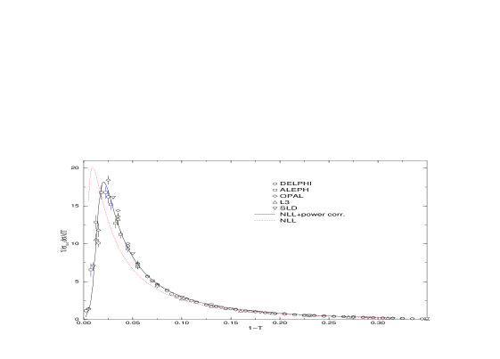
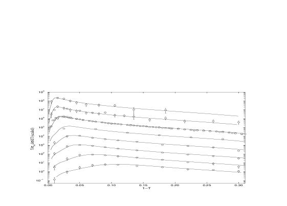
Figure 7: Fitting the shape function $\!{}^{{\bf?}}$ from the comparison with the data on the differential thrust distribution at $Q=91.2$ GeV.

Figure 8: Using the shape function $\!{}^{{\bf?}}$ to predict the differential thrust distribution at $Q=14,22,35,44,55,91,133,161$ GeV (from bottom to top).

In practice, one has to model the shape function using a certain ansatz and fit the parameters to describe the thrust distribution at a certain value of the c.m. energy $s=Q^{2}$. The result of such a fit is shown in Fig. 8. The energy dependence of the differential thrust distribution is then predicted without free parameters and appears to be in a good agreement with all available data, see Fig. 8.

The Energy Flow Correlation Function

The most important statement that has emerged from the application of renormalons to event shapes and is supported by all existing evidence is that soft-gluon emission presents the only source of linear $\Lambda/Q$ power corrections. This observation has profound consequences since emission of soft gluons occurs at time scales that are much larger than those involved in the formation of perturbative narrow jets. As a consequence, these two subprocesses are quantum-mechanically incoherent and the soft-gluon distribution emitted by a pair of quark jets at wide angles depends only on the direction and total color charge of the jets. This heuristic reasoning suggests factorization: to all orders in perturbation theory, inclusive cross sections for two narrow jets in $e^{+}e^{-}$ annihilation can be written as products of separate functions for the jets and the soft-gluon radiation, up to corrections suppressed by powers of $(\Lambda/Q)^{2}$. As a consequence, we can use the eikonal approximation and replace the jets by eikonal, or Wilson lines $W_{\pm}={\rm Pexp}[ig_{s}\int_{0}^{\infty}dup_{\pm}^{\mu}A_{\mu}(up_{\pm})]$ in which soft-gluon field is integrated along the light-like directions $p_{\pm}$ defined by the momenta of the outgoing jets. In this approximation the shape function for a given event shape variable $S$ becomes

$$\frac{1}{\sigma_{tot}}\frac{d\sigma_{NP}}{dS}=\sum_{N}|\langle N|W_{+}W_{-}^{\dagger}|0\rangle|^{2}\delta(S-S(N)),$$ (60)

where the sum goes over all final states and an UV cutoff $\mu$ is assumed for the gluon momenta.

The sum over the final states can be performed by introducing an operator ${\cal E}(\vec{n})$ that measures the density of energy flow in the direction of the unit vector $\vec{n}$ at spacial infinity. $\!{}^{{\bf?},{\bf?}}$ Then, in particular, the shape function for the thrust distribution becomes $\!{}^{{\bf?}}$

$$f_{t}(\epsilon)=\langle 0|(W_{+}W_{-}^{\dagger})(0)\,\delta\left(\epsilon-\int\!d\vec{n}\,w_{t}(\vec{n})\,{\cal E}(\vec{n},\mu)\right)(W_{-}W_{+}^{\dagger})(0)|0\rangle,$$ (61)

where $w_{t}(\vec{n})$ contains the information on the particular shape variable. In general, the complete information about soft-gluon emission is encoded in “multi-energy flow” correlation functions

$${\cal G}(\vec{n}_{1},\ldots,\vec{n}_{N};\mu)=\langle 0|(W_{+}W_{-}^{\dagger})(0)\,{\cal E}(\vec{n}_{1}),\ldots,{\cal E}(\vec{n}_{N})(W_{-}W_{+}^{\dagger})(0)|0\rangle$$ (62)

that describe the energy flow at spatial infinity. Power corrections to different event shape averages can be calculated in terms of the energy flow as

$$\langle S\rangle_{1/Q}=\int\!d\vec{n}\,w_{S}(\vec{n}){\cal G}(\vec{n},\mu).$$ (63)

The concept of energy flow is very useful, since it allows us to define the quantities of interest on an operator level, which makes them more amenable to a rigorous analysis of power corrections. On the other hand, many important issues remain to be resolved such as the dependence of the energy flow correlation functions on the factorization scale $\mu$. But already at the present stage the concept of energy flow has provided insights into the extent to which universality can be expected for power corrections to various moments or distributions of event shape observables.

3.3 Heavy Quarks

In this section we consider hard processes for which the large scale is given by the mass of a heavy quark. We discuss the notion of the (pole) mass of a heavy quark itself and its relation to the heavy quark potential, and consider applications of these results to $t\bar{t}$ pair production near the production threshold in $e^{+}e^{-}$ annihilation.

The Pole Mass

Since quarks are not observed as asymptotic states, their masses generally have to be considered as parameters in the QCD Lagrangian, on par with the strong coupling. Because the running of the coupling is conventionally considered using dimensional regularization, it is most natural to also employ the $\overline{\rm MS}$ scheme for the mass definition, introducing running quark masses $\bar{m}_{q}(\mu_{\overline{\rm MS}})$ and fixing their values at a certain reference scale. This is indeed the procedure used to deal with light quarks $q=u,d,s$ and also heavy quarks provided the hard scale in the process is larger than or of order of the quark mass. On the other hand, using $\overline{\rm MS}$ heavy quark masses is not convenient in processes where the hard scale is significantly smaller than the mass of the quark itself. The reason for this is that the usual renormalization group expression

$$m_{b}(\mu)\simeq\left(\frac{\alpha_{s}(\mu)}{\alpha_{s}(m_{b})}\right)^{4/b}m_{b}(m_{b})$$ (64)

is physically irrelevant at $\mu\ll m_{b}$ because it is derived by assuming that $\mu$ is the UV cutoff and thus the largest scale. (There is, formally, nothing wrong with taking $\mu\ll m_{b}$ in Eq. (64). However, in calculations of physical observables, e.g. heavy quark decay rates, we expect large perturbative corrections in higher orders in this case, because unphysical, large logarithms are generated.) On the other hand, in the limit $\mu\ll m_{b}$ the heavy quark interacts with gluons through the color Coulomb potential $V(\vec{r})=-C_{f}\alpha_{s}(1/r)/|\vec{r}|$. A restriction on the gluon momentum $|k|<\mu$ corresponds to the cutoff at large distances $r>1/\mu$ so that the dependence of the mass parameter on $\mu$ at $\Lambda\ll\mu\ll m_{b}$ is in fact linear $\!{}^{{\bf?},{\bf?},{\bf?}}$

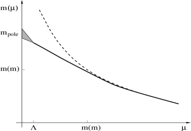
Figure 9: A schematic representation of the scale dependence of a heavy quark mass defined with a “physical” IR cutoff (solid line) and in the dimensional regularization (dashed line). The shaded area illustrates uncertainties of the mass definition when the scale is driven to values of order $\Lambda$

$$m_{b}(0)-m_{b}(\mu)\sim C_{f}\alpha_{s}\mu\,,$$ (65)

see Fig. 9 for an illustration. The quantity $m(0)$ would correspond to a “physical” quark mass if it existed and in perturbation theory can be defined as the location of the pole in the perturbative quark propagator, i.e. the pole mass:

$$m_{\rm pole}=m_{\overline{\rm MS}}(m_{\overline{\rm MS}})\left[1+\sum_{n}r_{n}\alpha_{s}^{n}(m_{\overline{\rm MS}})\right]$$ (66)

The pole mass is IR finite, gauge independent and independent on the renormalization scheme. $\!{}^{{\bf?},{\bf?}}$ The perturbative series in Eq. (66) is, however, divergent: $\!{}^{{\bf?},{\bf?},{\bf?}}$

$$r_{n}\sim\mbox{\rm const}\cdot(2\beta_{0})^{n}\Gamma[n+1+\beta_{1}/(2\beta_{0})^{2}].$$ (67)

The sum of the series is ambiguous by an amount of order $\Lambda$, and, therefore, the quark pole mass is perturbatively defined only to an accuracy

$$\delta m_{\rm pole}\sim\Lambda.$$ (68)

This uncertainty has important practical implications as it means that the pole mass has to be eliminated as a parameter in calculations of physical observables, if these observables are less sensitive to the IR region than the pole mass itself. Important examples of such observables are inclusive heavy quark decays $\!{}^{{\bf?},{\bf?},{\bf?},{\bf?},{\bf?},{\bf?}}$ and top quark production near threshold in $e^{+}e^{-}$ annihilation. The second example will be discussed in some detail below. IR renormalons have also been investigated for exclusive heavy quark decays, $\!{}^{{\bf?},{\bf?}}$ in which a relation with the heavy quark pole mass emerges through the binding energy $\bar{\Lambda}$, defined in heavy quark effective theory.

The Heavy Quark Mass with IR Subtractions.

In order to deal with a well-defined non-perturbative parameter and at the same time to retain the attractive features of the pole mass we have to perform an explicit scale separation. Heuristically, this would mean that the perturbative contributions in Eq. (66) have to be calculated using a cutoff $\mu$ at small momenta. The dependence of such subtracted mass on $\mu$ is linear and the coefficient depends on the particular procedure to implement the IR-cutoff, but it is difficult in practice to implement such a procedure, and to maintain gauge invariance in particular.

One suggestion $\!{}^{{\bf?}}$ has been to utilize a close connection between ambiguities in the pole mass and the static heavy quark potential. The starting observation $\!{}^{{\bf?}}$ is that the leading IR power correction to the potential in momentum space cannot be $\Lambda/|\vec{q}\,|$, but has to be quadratic:

$$\tilde{V}(\vec{q}\,)=-\frac{4\pi C_{F}\alpha_{s}(\vec{q}\,)}{\vec{q}^{\,2}}\left(1+\ldots+\,{\rm const}\cdot\frac{\Lambda^{2}}{\vec{q}^{\,2}}+\ldots\right).$$ (69)

To avoid misunderstanding, note that we are not concerned with the long-distance behaviour of the potential at $q\sim\Lambda$, but with the leading power corrections of the form $(\Lambda/q)^{k}$, which correct the perturbative Coulomb potential when $q$ is still large compared to $\Lambda$.

When we consider the coordinate space potential, given by the Fourier transform of $\tilde{V}(\vec{q}\,)$, a new situation arises. It is easy to see by dimensional analysis that the contribution of small $|q|<\mu$ in the Fourier integral is a $r$-independent constant:

$$\int\limits_{|\vec{q}\,|<\mu_{f}}\!\!\!\frac{d^{3}\vec{q}}{(2\pi)^{3}}\,e^{iq\cdot r}\tilde{V}(\vec{q}\,)\sim\int\limits_{|\vec{q}\,|<\mu_{f}}\!\!\!\frac{d^{3}\vec{q}}{(2\pi)^{3}}\,\tilde{V}(\vec{q}\,)=\mbox{\rm const}\cdot\mu\,.$$ (70)

This implies a long-distance and hence non-perturbative correction

$$V(r)=-\frac{C_{F}\alpha_{s}(1/r)}{r}\left(1+\ldots+\,{\rm const}\cdot\Lambda r+\ldots\right)$$ (71)

for the coordinate space potential that can also be observed through the calculation of renormalons generated by one-gluon exchange with vacuum polarization insertions. $\!{}^{{\bf?},{\bf?}}$

The $r$-independent constant in the potential is closely related to the uncertainty in the pole mass. This is easy to understand since the total energy of a heavy quark-antiquark system $E(r)=2m_{\rm pole}+V(r)$ is a physical observable and has to be well defined in the heavy quark limit. $\!{}^{{\bf?},{\bf?}}$ We can then define a potential-subtracted (PS) quark mass and a subtracted potential as $\!{}^{{\bf?}}$

$$m_{\rm PS}(\mu_{f}) = m_{\rm pole}-\delta m(\mu_{f}).$$

$$V(\vec{r},\mu_{f}) = V(\vec{r}\,)+2\delta m(\mu_{f})$$ (72)

where

$$\delta m(\mu_{f})=-\frac{1}{2}\int\limits_{|\vec{q}\,|<\mu_{f}}\!\!\!\frac{d^{3}\vec{q}}{(2\pi)^{3}}\,\tilde{V}(\vec{q}\,).$$ (73)

To 2-loop accuracy, the relation of the PS mass to $\bar{m}\equiv\bar{m}_{\overline{\rm MS}}(\bar{m}_{\overline{\rm MS}})$ is given by

$$m_{\rm PS}(\mu_{f}) = \bar{m}\,\Bigg{\{}1+\frac{4\alpha_{s}(\bar{m})}{3\pi}\left[1-\frac{\mu}{\bar{m}}\right]$$ (74)

$$+\left(\frac{\alpha_{s}(\bar{m})}{\pi}\right)^{2}\left[K_{1}-\frac{\mu}{3\bar{m}}\left(K_{2}-4\pi\beta_{0}\left[\ln\frac{\mu^{2}}{\bar{m}^{2}}-2\right]\right)\right]+\ldots\Bigg{\}},$$

where $K_{1}=13.44-1.04N_{f}$ is the 2-loop coefficient in the relation of $m_{\rm pole}$ to $\bar{m}$ $\!{}^{{\bf?}}$ and $K_{2}=10.33-1.11N_{f}$ the 1-loop correction to the Coulomb potential in momentum space. (The 3-loop relation is also known.) The important point is that in the perturbative expansion that relates the two masses in Eq. (74) the leading IR renormalon divergence has been eliminated. In practice, this leads to smaller perturbative coefficients starting already at two loops.

We can use the PS mass and subtracted potential instead of the pole mass and the Coulomb potential to perform Coulomb resummations for threshold problems. The benefit of using an unconventional mass definition is that large perturbative corrections related to strong renormalon divergence associated with the coordinate space potential are obviated. Physically, the crucial point is that, contrary to intuition, heavy quark cross sections near threshold are in fact less long-distance sensitive than the pole mass and the coordinate space potential. The cancelation is made explicit by using a less long-distance sensitive mass definition.

Top Quark Production in $e^{+}e^{-}$ Annihilation

It is perhaps surprising that the renormalon divergence in the pole mass/$\overline{\rm MS}$ mass relation and the mass subtractions discussed above have played a very important role for the top quark, which is so much heavier than the QCD scale. The reason for this is the extraordinary precision of about $100\,$MeV with which the top quark mass can in principle be determined by scanning the pair production threshold at an $e^{+}e^{-}$ collider.

The improvement in convergence due to the subtraction term can be seen on the one hand in the perturbative conversion to the $\overline{\rm MS}$ mass, and in the $t\bar{t}$ line shape on the other hand. Numerically, the series that relate the pole and PS mass, respectively, to the $\overline{\rm MS}$ mass $\bar{m}_{t}=\bar{m}_{t}(\bar{m}_{t})$ are as follows:

$$m_{t}=\big{[}165.0+7.64+1.64+0.52+0.25\,(\mbox{est.})\big{]}\,\mbox{GeV}$$ (75)

$$m_{t,\rm PS}(20\,\mbox{GeV})=\big{[}165.0+6.72+1.21+0.29+0.08\,(\mbox{est.})\big{]}\,\mbox{GeV}.$$ (76)

for $\bar{m}_{t}=165\,$GeV and $\alpha_{s}(\bar{m}_{t})=0.1091$ (corresponding to $\alpha_{s}(m_{Z})=0.119$). The 3-loop coefficients can also be computed using recent results. $\!{}^{{\bf?},{\bf?}}$ The 4-loop estimate uses the “large-$\beta_{0}$” limit. $\!{}^{{\bf?}}$ The improved convergence is evident and significant on the scale of $100\,$MeV set by the projected uncertainty on the mass measurement.

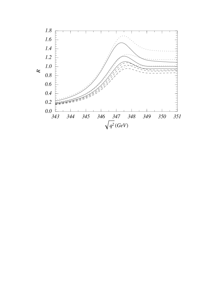
Figure 10: The total normalized $t\bar{t}$ cross section (virtual photon contribution only) in the threshold region at leading order (dotted), next-to-leading order (dashed) and next-to-next-to-leading order (NNLO) versus the center-of-mass energy. $\!{}^{{\bf?}}$ Both plots use $\bar{m}_{t}(\bar{m_{t}})=165\,$GeV, $\Gamma_{t}=1.43\,$GeV and $\alpha_{s}(m_{Z})=0.119$ as input. The three curves for each case refer to the renormalization scale $\mu=\left\{15(\mbox{upper});30(\mbox{central});60(\mbox{lower})\right\}\,$GeV. The PS mass corresponding to $\bar{m}_{t}(\bar{m_{t}})=165\,$GeV is $m_{t,\rm PS}(20\,\mbox{GeV})=173.30\,$GeV, the pole mass $m_{t,{\rm pole}}=175.05\,$GeV. The upper panel shows the successive approximations in the PS mass scheme, the lower panel in the pole mass scheme.

The calculation of the top quark pair production cross section near threshold uses a non-relativistic effective theory to accomplish the all-order resummation of Coulomb “singularities”. We cannot go into details here except to mention that the leading order cross section $\!{}^{{\bf?}}$ can be obtained from the effective Lagrangian

$${\cal L}_{\rm eff} = \psi^{\dagger}\left(i\partial^{0}+\delta m_{t}(\mu_{f})+\frac{\vec{\partial}^{2}}{2m_{t}}+i\Gamma_{t}\right)\psi$$ (77)

$$+\,\chi^{\dagger}\left(i\partial^{0}+\delta m_{t}(\mu_{f})-\frac{\vec{\partial}^{2}}{2m_{t}}+i\Gamma_{t}\right)\chi$$

$$+\,\int d^{d-1}r\left[\psi^{\dagger}\psi\right](r)\left(-\frac{C_{F}\alpha_{s}}{r}\right)\left[\chi^{\dagger}\chi\right](0),$$

where $\psi$ and $\chi$ denote non-relativistic quark and antiquark fields, respectively. The leading order Coulomb potential is part of the leading order Lagrangian and cannot be treated as a perturbative interaction term. The effective Lagrangian yields the Schrödinger equation for the $t\bar{t}$ system, the only peculiarity being that the Schrödinger equation contains a non-hermitian term to account for top quark decay and a residual mass term $\delta m_{t}(\mu_{f})$ defined by Eq. (73). The residual mass implies that the non-relativistic static energy is $\sqrt{q^{2}}-2m_{t,\rm PS}(\mu_{f})$ rather than $\sqrt{q^{2}}-2m_{t}$ and by expressing the cross section in terms of $\sqrt{q^{2}}-2m_{t,\rm PS}(\mu_{f})$, the convergence of the perturbative approximation is also improved here.

The cross section near threshold is now known to next-to-next-to-leading order $\!{}^{{\bf?},{\bf?},{\bf?},{\bf?},{\bf?}}$ and it is at this order that the improvement of convergence of the peak of the line shape becomes particularly visible, $\!{}^{{\bf?},{\bf?},{\bf?}}$ as shown in Fig. 10. Subtracted top quark masses are therefore essential to take profit from the small experimental error. As shown above the subtracted masses can be accurately converted to the $\overline{\rm MS}$ mass which should then be a useful standard. Subtractions different $\!{}^{{\bf?},{\bf?}}$ from the potential subtraction can be conceived and are useful as far as they eliminate the leading infrared sensitive term from the pole mass. They have also been used in top quark production. $\!{}^{{\bf?},{\bf?}}$

3.4 Synopsis of Other Results

The analysis of renormalon divergences can be used to study non-perturbative corrections to many other hard QCD processes. The following gives an incomplete discussion of some of these processes.

Fragmentation in $e^{+}e^{-}$ annihilation. Inclusive single particle production in $e^{+}e^{-}$ annihilation is the time-like analogue of deep inelastic scattering. A renormalon analysis $\!{}^{{\bf?},{\bf?},{\bf?}}$ predicts the leading power corrections to the differential cross section to be of order $(\Lambda/Q)^{2}$, in agreement with the light-cone expansion, $\!{}^{{\bf?}}$ and suggests the following parametrization:

$$\frac{d\sigma_{L}^{\rm tw-4}}{dx}(x,Q^{2}) = \frac{\Lambda^{2}}{Q^{2}}\!\int_{x}^{1}\!\frac{dz}{z}\,\Bigg{\{}c_{q}^{L}\left[\delta(1-z)+\frac{2}{z}\right]D_{q}(x/z,\mu)$$ (78)

$$\,+c_{g}^{L}\,\frac{1-z}{z^{3}}D_{g}(x/z,\mu)\Bigg{\}}~{},$$

$$\frac{d\sigma_{L+T}^{\rm tw-4}}{dx}(x,Q^{2}) = \frac{\Lambda^{2}}{Q^{2}}\!\int_{x}^{1}\!\frac{dz}{z}\Bigg{\{}c_{q}^{L+T}\!\left[\frac{-2}{[1-z]_{+}}+1+\frac{1}{2}\delta^{\prime}(1-z)\right]D_{q}(x/z,\mu)$$ (79)

$$\,+\left[c_{g}^{L+T}\,\frac{1-z}{z^{3}}+d\right]D_{g}(x/z,\mu)\Bigg{\}},$$

where $D_{i}$ denotes the leading-twist fragmentation function for parton $i$ to decay into any hadron, “$L$+$T$” the sum of longitudinal and transverse fragmentation cross sections and the plus distribution is defined as usual. The power corrections are added to the leading-twist cross sections as

$$\frac{d\sigma_{P}}{dx}(x,Q^{2})=\frac{d\sigma_{P}^{\rm tw-2}}{dx}(x,Q^{2})+\frac{d\sigma_{P}^{\rm tw-4}}{dx}(x,Q^{2}).$$ (80)

The constants $c_{k}$ and $d$ are to be fitted to data and depend on the order of perturbation theory and factorization scale $\mu$ adopted for the leading-twist prediction.

Owing to energy conservation, the parton fragmentation functions disappear from the second moments

$$\sigma_{L,T}\equiv\sum_{H}\frac{1}{2}\int_{0}^{1}\!dx\,x\frac{d\sigma_{L,T}^{H}}{dx},$$ (81)

which can therefore be calculated in perturbation theory up to power corrections. The power expansion of the fragmentation cross section has strong soft-gluon singularities and the expansion parameter relevant at small $x$ is $\Lambda^{2}/(Q^{2}x^{2})$. This can be related to the fact that in perturbation theory the hard scale relevant to gluon fragmentation is not $Q$, but the energy $Qx$ of the fragmenting gluon. It was noted $\!{}^{{\bf?},{\bf?}}$ that these strong singularities lead to a linear $\Lambda/Q$ non-perturbative correction to the $\sigma_{L}$ and $\sigma_{T}$. This can be seen from

$$\int\limits_{\Lambda/Q}dx\,\frac{1}{2}\,x\left[\frac{\Lambda^{2}}{Q^{2}x^{2}}\right]^{n}\sim\frac{\Lambda}{Q}$$ (82)

for any $n$, which also tells us that the correct $1/Q$ power correction is obtained only after resumming the power expansion at definite $x$ to all orders. To the 2-loop accuracy, the IR contribution to $\sigma_{L}$ appears to be related to that for the $C$-parameter. $\!{}^{{\bf?}}$

The total cross section in $e^{+}e^{-}$ annihilation into hadrons is given by the sum of the transverse and longitudinal cross section. In this sum all power corrections of order $1/Q$, $1/Q^{2}$ and $1/Q^{3}$ cancel as expected from the operator product expansion.

Drell-Yan production. Drell-Yan production of a lepton pair or a massive vector boson, $A+B\to\{\gamma^{*},W,Z\}(Q)+X$, where $X$ is any hadronic final state, presents the best studied case of a hard process with two disparate hard scales for which logarithmically enhanced contributions due to soft-gluon emission can be resummed systematically to all orders of perturbation theory. $\!{}^{{\bf?},{\bf?}}$ In Mellin space, the cross section $d\sigma_{\rm DY}/dQ^{2}$ factorises into a product of parton distribution functions and the quark-antiquark scattering cross section that takes the form

$$\omega_{q\bar{q}}(N,\alpha_{s}(Q))=H(\alpha_{s}(Q))\,\exp\left[E(N,\alpha_{s}(Q))\right]+R(N,\alpha_{s}(Q)),$$ (83)

where $R(N,\alpha_{s}(Q))$ vanishes as $N\to\infty$, $H(\alpha_{s}(Q))$ is independent of $N$, and the exponent is given by

$$E(N,\alpha_{s}(Q))\!\! = \!\!\int_{0}^{1}dz\,\frac{z^{N-1}-1}{1-z}\,\Bigg{\{}2\int_{Q^{2}(1-z)}^{Q^{2}(1-z)^{2}}\!\!\frac{dk_{t}^{2}}{k_{t}^{2}}\,\Gamma[\alpha_{s}(k^{2}_{t})]$$ (84)

$$\hskip 28.45274pt{}+\,B[\alpha_{s}((1\!-\!z)Q^{2})]+C[\alpha_{s}((1\!-\!z)^{2}Q^{2})]\Bigg{\}}.$$

A similar expression is valid for the thrust distribution, cf. Eq. (55), in which case we argued that it implies a linear in $1/Q$ non-perturbative correction because of the corresponding IR sensitivity of the first term involving the integral of the QCD coupling over low scales. For Drell-Yan production it happens, however, that the infrared renormalon contributions arising in this way $\!{}^{{\bf?}}$ are exactly canceled by the divergent perturbative expansion of the function $C[\alpha_{s}]$. $\!{}^{{\bf?}}$ The cancelation was shown explicitly in the large-$\beta_{0}$ approximation and can be interpreted $\!{}^{{\bf?}}$ as the cancelation of $O(1/Q)$ corrections between soft-gluon emission at different angles. In particular, the large-angle, non-collinear emission is important. This conclusion is general and extends beyond Drell-Yan process. A recent reanalysis $\!{}^{{\bf?}}$ of soft-gluon resummation in Drell-Yan production also arrives at the cancelation of the leading $1/Q$ IR contributions. The absense of $1/Q$ power corrections has been put $\!{}^{{\bf?},{\bf?},{\bf?}}$ into the more general context of Kinoshita-Lee-Nauenberg (KLN) cancelations. Knowing that any potential $1/Q$ correction would come from soft particles, but not collinear particles, the KLN transition amplitude can be constructed, which includes a sum over soft initial and final particles degenerate with the annihilating $q\bar{q}$ pair. The KLN transition amplitudes have no $1/k_{0}$ (where $k_{0}$ stands for the energies of the soft particles) contributions (collinear factorization is implicitly assumed). As a consequence, the amplitude squared, integrated unweighted over all phase space, is proportional to $dk_{0}k_{0}$, which by power counting implies at most $1/Q^{2}$ power corrections. To make connection with a physical process, one has to demonstrate that the sum over degenerate initial states can actually be dispensed of. This can be shown in an abelian theory using Low’s theorem. The generalization to QCD is still an open problem.

Hard exclusive reactions. The theory of hard exclusive scattering is much less developed compared to inclusive processes. Also from the experimental side there is conflicting evidence. In this situation simple estimates using renormalons can provide important insight. In a generic hard exclusive process one finds two sources of renormalon divergence and power corrections. The first is power corrections in the hard coefficient function, which are present independently of the form of the hadron wave function. These correspond to higher-twist corrections in the hard scattering formalism. Additional power corrections are generated after integrating with the hadron wave function over the parton momentum fractions and these depend on the details of the wave function. These power corrections arise from the region of small parton momentum fraction and can be associated with power corrections due to the “soft” or “Feynman” mechanism for exclusive scattering. For the simplest reaction $\!{}^{{\bf?}}$ $\gamma^{*}+\gamma\to\pi^{0}$ and the deeply virtual Compton scattering $\!{}^{{\bf?}}$ $\gamma^{*}+A\to\gamma+B$ both power corrections are of order $1/Q^{2}$. Another interesting application $\!{}^{{\bf?}}$ concerns the structure of the light-cone expansion of a non-local operator sandwiched between vacuum and the pion that is used to define the pion distribution amplitude $\phi_{\pi}(u)$:

$$\langle 0|\bar{d}(0)\gamma_{\mu}\gamma_{5}u(x)|\pi^{+}(p)\rangle\! = \!\!if_{\pi}p_{\mu}\!\int_{0}^{1}\!du\,e^{-iupx}\bigg{[}\bigg{(}1+\!\sum_{n}r_{n}(u)\alpha_{s}^{n}\bigg{)}\phi_{\pi}(u)$$ (85)

$$\hskip 56.9055pt+x^{2}g_{1}(u)+O(x^{4})\bigg{]}.$$

The function $g_{1}(u)$ is interpreted as a two-particle pion distribution function of twist-4 $\!{}^{{\bf?}}$ and is usually estimated to be $g_{1}(u)\sim\mbox{\rm const}\cdot u^{2}(1-u)^{2}$ by the contribution of the lowest conformal operator. The renormalon estimates can give constraints on possible contributions of high orders in the conformal expansion and in the large-$\beta_{0}$ limit the result is $\!{}^{{\bf?}}$ $g_{1}^{\rm ren}(u)\sim\mbox{\rm const}\cdot u(1-u)$. This result is significant since the behavior of $g_{1}(u)$ at the end points determines the parametric size of power corrections to inclusive reactions involving pions. In particular, a nonzero value $g_{1}(u\to 1)$ would invalidate factorization for the pion form factor. The further softening of the endpoint behavior $(1-u)\to(1-u)^{2}$ predicted by the conformal expansion must be interpreted as the effect of the hierarchy of the anomalous dimensions of conformal operators.

Deep inelastic scattering in the small-$x$ limit.  Exploratory studies $\!{}^{{\bf?},{\bf?}}$ have been performed in the context of small-$x$ structure functions to use renormalons in order to obtain a certain prescription to implement the running coupling in the BFKL equation. An apparent $1/Q$ correction to the kernel is suppressed $\!{}^{{\bf?}}$ after convolution with the hadron wave function such that the correction to the structure function is only of order $1/Q^{2}$. More recently, similar studies have been carried out involving the next-to-leading order BFKL kernel. $\!{}^{{\bf?},{\bf?}}$ The series expansion of the solution to the BFKL equation with the exact 1-loop running coupling produces a series expansion of the form $\!{}^{{\bf?}}$

$$\sum_{n}\left(ay\alpha_{s}^{3}\right)^{n/2}\,\Gamma(n/2),$$ (86)

where $a=42\zeta(3)\beta_{0}^{2}/\pi$ and $y$ is the (large) rapidity that characterizes a scattering process in the BFKL limit. If we take the Borel transform with respect to $\alpha_{s}^{3}$, the above series leads to a typical renormalon pole. The unusual feature is that location of the renormalon pole depends on the kinematic variable $y$, and not only in overall prefactor. When $ay\alpha_{s}^{3}\sim 1$ the series diverges from the outset and no perturbative approximation is possible. This leads to the constraint $y<1/(a\alpha_{s}^{3})$ for rapidities to which the BFKL treatment can be applied, in agreement with other methods. $\!{}^{{\bf?}}$

4 Ultraviolet Renormalons

Perturbative expansions in renormalizable field theories exhibit another kind of divergence known as the ultraviolet (UV) renormalon. This divergence is easy to identify in simple sets of diagrams. For example, the integral in Eq. (5) has a contribution of order $(-\beta_{0}/q)^{n}n!$ from large $k\gg Q$, where $q$ depends on the behavior of $I(k)$ at large $k$. For UV finite or renormalized quantities the leading term $I(k)\sim 1/k^{4}$ is absent or subtracted and $I(k)\sim 1/k^{6}$ in general. This leads to $q=1$. Higher orders in the large-$k$ expansion of $I(k)$ give rise to divergent behavior with larger $q$ and the corresponding singularities in the Borel transform.

We note that since $k\gg Q$ the powers of the logarithm in Eq. (5) alternate in sign. Hence the terms of the divergent series are also sign-alternating. For such series the Borel integral can be unambiguously defined and so it seems that we need not concern ourselves further with this type of divergence. However, it is not obvious that Borel summation is the correct way to recover the non-perturbative result. The series alone tells us only that we can approximate the exact result up to an uncertainty of order $(\Lambda/Q)^{2}$, if $q=1$ and if the series expansion is expressed in terms of $\alpha_{s}(Q)$.

This is a puzzling result. For the GLS sum rule $I_{\rm GLS}$, used as an example in the introduction, this implies an ambiguity from arbitrarily large loop momenta as large as the leading higher-twist correction, even though the strong coupling is small in the ultraviolet. And how could such an UV effect be non-local (non-polynomial) in the external momentum $Q$? We shall see later in this section that the estimate $(\Lambda/Q)^{2}$ is too naive and that there is indeed no ambiguity associated with UV renormalons. But we shall first discuss the theory of UV renormalons independent of particular sets of diagrams.

UV renormalons are related to internal loop momenta larger than any external momentum; they disappear if Green functions are computed with a UV cutoff not taken to infinity. This suggests that the methods of renormalization theory can be used to characterize UV renormalons. The simple example of the function $I(k)$ discussed above shows that the first UV renormalon ($q=1$) is related to dimension-6 operators, since this is what the first non-vanishing term in the large-$k$ expansion would yield. The first UV renormalon is particularly simple since for dimensional reasons we can allow only a single insertion of a dimension-6 operator. Parisi $\!{}^{{\bf?}}$ has used this insight to compute the nature of the leading UV renormalon singularity in the scalar $\phi^{4}$-theory; the connection with effective theories at finite UV cutoff was also pursued. $\!{}^{{\bf?}}$ Later particular sets of diagrams were investigated $\!{}^{{\bf?},{\bf?},{\bf?},{\bf?}}$ and the dimension-6 operators corresponding to them were identified. In particular, the dominant role of four-fermion operators was emphasized by Vainshtein and Zakharov. $\!{}^{{\bf?}}$

Parisi’s method can be used to determine the UV renormalon singularity in QCD up to an overall constant $\!{}^{{\bf?}}$ by means of renormalization group equations. These equations are formulated most easily for ambiguities or, equivalently, imaginary parts of Borel-type integrals. In QCD UV renormalons lie on the negative Borel axis and do not lead to ambiguities. It is technically convenient to consider instead the integral

$$I[R](\alpha_{s})=\int\limits_{0+i\epsilon}^{-t_{c}+i\epsilon}dt\,e^{-t/\alpha_{s}}\,B[R](t)\qquad 0<\frac{1}{\beta_{0}}<t_{c}<\frac{2}{\beta_{0}},$$ (87)

given a series expansion $R$ in $\alpha_{s}=\alpha_{s}(\mu)$ and its Borel transform $B[R](t)$. The integral is complex and its imaginary part is unambiguously related to the first UV renormalon singularity at $t=-1/\beta_{0}$ or the corresponding large-order behavior.

The UV factorization properties of Green functions imply that the imaginary part of $I[R]$ owing to the leading UV renormalon can be represented as

$$\mbox{Im}\,I[R](\alpha_{s},p_{k})=\frac{1}{\mu^{2}}\sum_{i}C_{i}(\alpha_{s})\,R_{{\cal O}_{i}}(\alpha_{s},p_{k}).$$ (88)

In this equation ${\cal O}_{i}$ denote dimension-6 operators and $R_{{\cal O}_{i}}$ the Green function from which $R$ is derived with a single zero-momentum insertion of ${\cal O}_{i}$. $C_{i}(\alpha_{s})$ are the coefficient functions, which are independent of any external momentum $p_{k}$ of $R$ and in fact independent of the quantity $R$. They play the same role as the universal renormalization constants in ordinary renormalization. The coefficient function being universal, the dependence of the UV renormalon divergence on the observable $R$ is contained in the factors $R_{{\cal O}_{i}}$. These factors can be computed order by order in $\alpha_{s}$ by conventional methods. We will not prove Eq. (88) here, but rely on the fact that familiarity with ordinary renormalization will make it appear plausible.

The dimension-6 operators may be thought of as an additional term,

$$\Delta{\cal L}=-\frac{i}{\mu^{2}}\sum_{i}C_{i}(\alpha_{s})\,{\cal O}_{i},$$ (89)

in the QCD Lagrangian with coefficients such that for any $R$ the imaginary part of $I[R]$ is compensated by the additional contribution to $R$ from $\Delta{\cal L}$. From the requirement that $\Delta{\cal L}$ be independent of the renormalization scale $\mu$ or from a comparison of the renormalization group equations satisfied by $I[R]$ and $R_{{\cal O}_{i}}$ it can be derived that

$$\left[\left(\beta(\alpha_{s})\frac{d}{d\alpha_{s}}-1\right)\delta_{ij}-\frac{1}{2}\gamma_{ij}(\alpha_{s})\right]C_{j}(\alpha_{s})=0,$$ (90)

where $\gamma(\alpha_{s})$ is the anomalous dimension matrix of the dimension-6 operators defined such that the renormalized operators satisfy

$$\left(\delta_{ij}\,\mu\frac{d}{d\mu}+\gamma_{ij}\right){\cal O}_{j}=0.$$ (91)

The unusual “$-1$” in Eq. (90) originates from the factor $1/\mu^{2}$ in Eq. (88). The solution to the differential equation (90) can be written as

$$C_{i}(\alpha_{s})=e^{1/(\beta_{0}\alpha_{s})}\alpha_{s}^{\beta_{1}/\beta_{0}^{2}}\,F(\alpha_{s})\,E_{i}(\alpha_{s}),$$ (92)

where

$$F(\alpha_{s})=\exp\left(\,\int_{0}^{\alpha_{s}}dx\left[-\frac{1}{\beta_{0}x^{2}}+\frac{\beta_{1}}{\beta_{0}^{2}x}-\frac{1}{\beta(x)}\right]\right)$$ (93)

has a regular series expansion in $\alpha_{s}$ and incorporates the effect of terms of higher order than $\beta_{1}$ in the $\beta$-function and

$$E_{i}(\alpha_{s})=\exp\left(\,\int_{\alpha_{0}}^{\alpha_{s}}dx\,\frac{\gamma_{ij}^{T}(x)}{2\beta(x)}\right)\hat{C}_{j}$$ (94)

takes into account the (transpose of the) anomalous dimension matrix. Thus, the coefficient functions are determined up to $\alpha_{s}$-independent integration constants $\hat{C}_{i}$. (The lower limit $\alpha_{0}$ in Eq. (94) is arbitrary. A change of $\alpha_{0}$ can be compensated by adjusting the integration constants.) Because the $\alpha_{s}$-dependence in Eq. (87) translates into $n$-dependence of large-order behavior, we deduce that this $n$-dependence is completely determined. Only overall normalization factors related to the integration constants do not follow from the renormalization group equation. However, these integration constants are process-independent numbers; they depend only on the Lagrangian that specifies the theory. It is in this precise sense that ultraviolet renormalon divergence is universal. This should be contrasted to the case of IR renormalons, which depend not only on the Lagrangian, but also on other IR parameters relevant to a specific class of processes.

We now specify a basis of dimension-6 operators. In general, we are also interested in processes induced by external currents. Here we consider only vector and axial-vector currents and we let them be flavor singlets. Thus, in expressions like $(\bar{\psi}M\psi)$, a sum over flavor, color and spinor indices is implied, and $M$ is a matrix in color and spinor space, but unity in flavor space. To account for the external currents, two (abelian) background fields $v_{\mu}$ and $a_{\mu}$, which couple to the vector and axial-vector current, are introduced. Their fields strengths $F_{\mu\nu}=\partial_{\mu}v_{\nu}-\partial_{\nu}v_{\mu}$ and $H_{\mu\nu}=\partial_{\mu}a_{\nu}-\partial_{\nu}a_{\mu}$ satisfy $\partial_{\mu}F^{\mu\nu}=j_{V}^{\nu}$ and $\partial_{\mu}H^{\mu\nu}=j_{A}^{\nu}$. A basis of dimension-6 operators is then given by

$${\cal O}_{1} = (\bar{\psi}\gamma_{\mu}\psi)(\bar{\psi}\gamma^{\mu}\psi)\qquad\qquad\,\,\,{\cal O}_{2}\,=\,(\bar{\psi}\gamma_{\mu}\gamma_{5}\psi)(\bar{\psi}\gamma^{\mu}\gamma_{5}\psi)$$

$${\cal O}_{3} = (\bar{\psi}\gamma_{\mu}T^{A}\psi)(\bar{\psi}\gamma^{\mu}T^{A}\psi)\qquad\!\!{\cal O}_{4}\,=\,(\bar{\psi}\gamma_{\mu}\gamma_{5}T^{A}\psi)(\bar{\psi}\gamma^{\mu}\gamma_{5}T^{A}\psi)$$

$${\cal O}_{5} = \frac{1}{g_{s}}\,f_{ABC}\,G_{\mu\nu}^{A}G_{\rho}^{\nu\,B}G^{\rho\mu\,C}$$ (95)

$${\cal O}_{6} = \frac{1}{g_{s}^{2}}\,(\bar{\psi}\gamma_{\mu}\psi)\,\partial_{\nu}F^{\nu\mu}\qquad{\cal O}_{7}\,=\,\frac{1}{g_{s}^{2}}\,(\bar{\psi}\gamma_{\mu}\gamma_{5}\psi)\,\partial_{\nu}H^{\nu\mu}$$

$${\cal O}_{8} = \frac{1}{g_{s}^{4}}\,\partial_{\nu}F^{\nu\mu}\,\partial^{\rho}F_{\rho\mu}\qquad\quad\!\!{\cal O}_{9}\,=\,\frac{1}{g_{s}^{4}}\,\partial_{\nu}H^{\nu\mu}\,\partial^{\rho}H_{\rho\mu},$$

where the overall factors $1/g_{s}^{k}$ have been inserted for convenience. We neglected gauge-variant operators and operators that vanish by the equations of motion. We also assume that all $N_{f}$ quarks are massless. Chirality then allows us to omit four-fermion operators of scalar, pseudo-scalar or tensor type. Diagrammatically, they cannot be generated in massless QCD, because the number of Dirac matrices on any fermion line that connects to an external fermion in a four-point function is always odd.

To determine the leading asymptotic behavior we only need the leading term in $\alpha_{s}$ of Eq. (88). To this order $F(\alpha_{s})=1$ and only the leading order anomalous dimension matrix is needed to compute the factors $E_{i}(\alpha_{s})$. We will not present this calculation $\!{}^{{\bf?}}$ in detail here, but discuss briefly the structure of the result for the correlation function of two vector currents, $\Pi(Q)$. The leading contribution is caused by mixing of the four-quark operators into the operator ${\cal O}_{8}$. Taking into account that $\Pi(Q)_{{\cal O}_{8}}(\alpha_{s},Q)\propto\alpha_{s}^{-2}$ at leading order, we obtain

$$\mbox{Im}\,I[\Pi](\alpha_{s},Q)\propto\frac{Q^{2}}{\mu^{2}}\,e^{1/(\beta_{0}\alpha_{s})}\alpha_{s}^{-2-\lambda_{1}+\beta_{1}/\beta_{0}^{2}}(1+O(\alpha_{s})),$$ (96)

where $\lambda_{1}$ is related to the largest eigenvalue of the anomalous dimension matrix of the four-quark operators. Converting the previous equation into large-order behavior gives, taking $\mu=Q$,

$$r_{n}\stackrel{{\scriptstyle n\to\infty}}{{=}}K\,(-\beta_{0})^{n}\,n!\,n^{2-\beta_{1}/\beta_{0}^{2}+\lambda_{1}}=K\,(-\beta_{0})^{n}\,n!\,n^{\{1.59,1.75,1.97\}},$$ (97)

for $N_{f}=\{3,4,5\}$. The constant $K$ is related to the integration constants $\hat{C}_{j}$ and it is not known how to compute it. The result generalizes to a non-flavor-symmetric vector current with a different constant $K$.

It is interesting to note that subleading corrections to the asymptotic behavior can be computed without introducing further “non-perturbative” parameters in addition to the constants $\hat{C}_{i}$ already present at leading order. As a rule, to obtain the coefficient of the $1/n^{k}$ correction, one needs the $\beta$-function coefficients $\beta_{0},\ldots,\beta_{k+1}$, the $(k+1)$-loop anomalous dimension matrix and the $k$-loop correction to Green functions with operator insertions. The renormalization group treatment can in principle be extended to the next singularity in the Borel plane at $t=-2/\beta_{0}$, but this is far more complicated, since single insertions of dimension-8 operators and double insertions of dimension-6 operators would have to be taken into account.

Now that we know how to compute UV renormalons we return to the question whether there exist power corrections associated with them. Equation (96) shows that the power-suppressed imaginary part is, after all, polynomial in $Q$. Keeping the renormalization scale $\mu$ and $Q$ different, we then find that the minimal term of the UV renormalon series scales as $\!{}^{{\bf?}}$

$$\frac{Q^{2}}{\mu^{2}}\,\frac{\Lambda^{2}}{\mu^{2}}\times[\mbox{powers of }\alpha_{s}]$$ (98)

rather than $(\Lambda/Q)^{2}$. Since $\mu$ is an arbitrary parameter we are free to make it large. The effects of this is to delay the onset of UV renormalon divergence, as the minimal term of the series occurs at order $n\sim 1/(\beta_{0}\alpha_{s}(\mu))$, and to simultaneously render the minimal term small. (If the number of known terms in the series is small, this is not a practical way to deal with UV renormalons. In this case one can make use of conformal mappings in the Borel plane to render the UV renormalon singularities less important. $\!{}^{{\bf?},{\bf?},{\bf?}}$) Essentially this phenomenon occurs because the natural scale of the UV renormalon divergence is much larger than $Q$. By adjusting $\mu$ in this way, we decrease the perturbative coefficients. Since the strong coupling also decreases, the UV renormalon divergence becomes irrelevant. This is to be contrasted with the case of IR renormalons in which case $\mu$ would have to be adjusted to low values. As the perturbative coefficients decrease, the coupling increases and both effects exactly compensate each other as far as the minimal term of the series is concerned. Note that these purely perturbative considerations do not imply that there cannot be any non-perturbative power correction associated with short distances. But they tell us that whatever these corrections are they bear no relation with UV renormalons.

5 Conclusion

During the past few years infrared renormalons have emerged as a useful tool for the analysis of IR contributions to Feynman diagrams beyond the leading power in the perturbative scale, and, by implication, for the analysis of non-perturbative power corrections to generic hard processes.

In this review we have given a brief survey of the basic ideas and considered a few selected applications of the method, which we think are the most relevant. An important problem that we have not discussed is the relation of renormalons to lattice calculations in general and in particular to non-perturbative lattice renormalization procedures for higher-twist operators. Possible non-perturbative corrections coming from small distances (e.g. due to instanton contributions) have also been left out.

We attempted to emphasize that the subject of IR renormalons is closely related to the extension of QCD factorization theorems on logarithmic IR singularities to leading power corrections in the hard scale. This extended factorization is at present well understood only at the 1-loop level (e.g. for event shapes). An outstanding problem that remains even at this level is to compute the (leading) logarithmic corrections to the power behavior. In the few cases for which the result is known, its derivation is based on the operator product expansion and the calculation of the anomalous dimensions of the relevant higher-twist operators. The extension to event shapes would require an understanding of the renormalization group equations for the corresponding shape functions (cf. Sect. 3) that have yet to be written down.

An important formal problem that remains is the calculation of the overall constants of the large-order behavior. This task cannot be addressed within perturbation theory itself and requires new methods. Some recent developments $\!{}^{{\bf?},{\bf?}}$ may be interesting in this respect, but it appears unlikely that an exact analytic solution can be found.

References

References

- [1] M. Beneke, Phys. Rept. 317, 1 (1999).
- [2] D.J. Gross and A. Neveu, 1974, Phys. Rev. D 10, 3235 (1974).
- [3] B. Lautrup, Phys. Lett. B 69, 109 (1977).
- [4] G. ‘t Hooft in The Whys of subnuclear physics, Proc. Int. School, Erice, Italy, 1977, ed. A. Zichichi (Plenum, New York, 1978).
- [5] F. David, Nucl. Phys. B 234, 237 (1984); ibid. B 263, 637 (1986).
- [6] V.A. Novikov, M.A. Shifman, A.I. Vainshtein and V.I. Zakharov, Nucl. Phys. B 249, 445 (1985).
- [7] A.H. Mueller, Nucl. Phys. B 250, 327 (1985).
- [8] G. Parisi, Phys. Lett. B 76, 65 (1978).
- [9] G. Parisi, Nucl. Phys. B 150, 163 (1979).
- [10] A.V. Manohar and M.B. Wise, Phys. Lett. B 344, 407 (1995).
- [11] K.G. Wilson, Phys. Rev. 179, 1499 (1969).
- [12] N. Christ, B. Hasslacher and A.H. Mueller, Phys. Rev. D 6, 3543 (1972).
- [13] M.A. Shifman, A.I. Vainshtein and V.I. Zakharov, Nucl. Phys. B 147, 385 (1979).
- [14] M. Beneke, Phys. Lett. B 307, 154 (1993).
- [15] G. Grunberg, Phys. Lett. B 304, 183 (1993).
- [16] F. David, Nucl. Phys. B 209, 433 (1982).
- [17] V.A. Novikov, M.A. Shifman, A.I. Vainshtein and V.I. Zakharov, Phys. Rept. 116, 104 (1984).
- [18] M.V. Terent’ev, Sov. J. Nucl. Phys. 45(2), 368 (1987); Fortschr. Phys. 36, 117 (1988).
- [19] M. Beneke, V.M. Braun and N. Kivel, Phys. Lett. B 443, 308 (1998).
- [20] M. Beneke, Nucl. Phys. B 405, 424 (1993).
- [21] D.J. Broadhurst, Z. Phys. C 58, 339 (1993).
- [22] M. Neubert, Phys. Rev. D 51, 5924 (1995).
- [23] V.I. Zakharov, Nucl. Phys. B 385, 452 (1992).
- [24] M. Beneke and V.I. Zakharov, Phys. Lett. B 312, 340 (1993).
- [25] M. Beneke and V.M. Braun, Phys. Lett. B 348, 513 (1995).
- [26] P. Ball, M. Beneke and V.M. Braun, Nucl. Phys. B 452, 563 (1995).
- [27] C.N. Lovett-Turner and C.J. Maxwell, Nucl. Phys. B 452, 188 (1995).
- [28] S.J. Brodsky, G.P. Lepage and P.B. Mackenzie, Phys. Rev. D 28, 228 (1983).
- [29] M. Beneke and V.M. Braun, Nucl. Phys. B 426, 301 (1994).
- [30] I.I. Bigi, M.A. Shifman, N.G. Uraltsev and A.I. Vainshtein, Phys. Rev. D 50, 2234 (1994).
- [31] B.R. Webber, Phys. Lett. B 339, 148 (1994).
- [32] G. Grunberg, Phys. Lett. B 372, 121 (1996).
- [33] Yu.L. Dokshitzer and N.G. Uraltsev, Phys. Lett. B 380, 141 (1996).
- [34] S. Peris and E. de Rafael, Phys. Lett. B 387, 603 (1996).
- [35] A.H. Mueller, Phys. Lett. B 308, 355 (1993).
- [36] M. Beneke, V.M. Braun and N. Kivel, Phys. Lett. B 404, 315 (1997).
- [37] X. Ji, Nucl. Phys. B 448, 51 (1995).
- [38] D.J. Broadhurst and A.L. Kataev, Phys. Lett. B 315, 179 (1993).
- [39] V.M. Braun and A.V. Kolesnichenko, Nucl. Phys. B 283, 723 (1987).
- [40] R.L. Jaffe and M. Soldate, Phys. Lett. B 105, 467 (1981); Phys. Rev. D 26, 49 (1982).
- [41] R.K. Ellis, W. Furmanski and R. Petronzio, Nucl. Phys. B 212, 29 (1983).
- [42] R.L. Jaffe, Nucl. Phys. B 229, 205 (1983).
- [43] I.I. Balitsky, and V.M. Braun, Nucl. Phys. B 311, 541 (1988/89).
- [44] M. Beneke and V.M. Braun, Nucl. Phys. B 454, 253 (1995).
- [45] Yu.L. Dokshitzer, G. Marchesini and B.R. Webber, Nucl. Phys. B 469, 93 (1996).
- [46] M. Maul, E. Stein, A. Schäfer and L. Mankiewicz, Phys. Lett. B 401, 100 (1997).
- [47] M. Beneke, V.M. Braun and L. Magnea, Nucl. Phys. B 497, 297 (1997).
- [48] U. K. Yang and A. Bodek, Phys. Rev. Lett. 82, 2467 (1999).
- [49] M. Dasgupta, and B.R. Webber, Phys. Lett. B 382, 273 (1996).
- [50] E. Stein, M. Meyer-Hermann, L. Mankiewicz and A. Schäfer, Phys. Lett. B 376, 177 (1996).
- [51] M. Meyer-Hermann, et al., Phys. Lett. B 383, 463 (1996) [Erratum: ibid. B 393, 487 (1997)].
- [52] E. Stein, M. Maul, L. Mankiewicz and A. Schäfer, Nucl. Phys. B 536, 318 (1998).
- [53] G. E. Smye, Nucl. Phys. B 546, 315 (1999).
- [54] M. Virchaux and A. Milsztajn, Phys. Lett. B 274, 221 (1992).
- [55] U. K. Yang and A. Bodek, Eur. Phys. J. C 13, 241 (2000).
- [56] G.T. Bodwin, S.J. Brodsky and G.P. Lepage, Phys. Rev. D 39, 3287 (1989).
- [57] A.L. Kataev, A.V. Kotikov, G. Parente and A.V. Sidorov, in Proceedings of the 32nd Rencontres de Moriond: QCD and High-Energy Hadronic Interactions, Les Arcs, France, 22-29 Mar 1997 [hep-ph/9706534].
- [58] A.L. Kataev, G. Parente and A.V. Sidorov, Nucl. Phys. B 573, 405 (2000).
- [59] S.A. Kulagin and A.V. Sidorov, hep-ph/0009150.
-
[60]
O. Biebel, hep-ex/0006020;
M. Acciarri et al. [L3 Collaboration], hep-ex/0005045;
G. Abbiendi et al. [JADE Collaboration], hep-ex/0001055;
G. Dissertori, Nucl. Phys. Proc. Suppl. 79, 438 (1999), [hep-ex/9904033];
P. Abreu et al. [DELPHI Collaboration], Phys. Lett. B 456, 322 (1999). - [61] F. Barreiro, Fortsch. Phys. 34, 503 (1986).
- [62] Yu.L. Dokshitzer and B.R. Webber, Phys. Lett. B 352, 451 (1995).
- [63] R. Akhoury and V.I. Zakharov, Phys. Lett. B 357, 646 (1995); Nucl. Phys. B 465, 295 (1996).
- [64] P. Nason and M.H. Seymour, Nucl. Phys. B 454, 291 (1995).
- [65] G.P. Korchemsky and G. Sterman, Nucl. Phys. B 437, 415 (1995).
- [66] G.P. Korchemsky and G. Sterman, in ’95 QCD and High Energy Hadronic Interactions, 30th Rencontres de Moriond, Meribel les Allues, France, 19-25 Mar 1995, J. Tran Thanh Van (ed.) (Editions Frontieres, 1995) [hep-ph/9505391].
- [67] P.A. Movilla Fernández et al. [The JADE Collaboration], Eur. Phys. J. C 1, 461 (1998).
- [68] M. Beneke and V.M. Braun, Nucl. Phys. Proc. Suppl. 51C, 217 (1996) [hep-ph/9605375].
- [69] J.M. Campbell, E.W.N. Glover and C.J. Maxwell, Phys. Rev. Lett. 81, 1568 (1998).
- [70] O. Biebel, hep-ex/0006020.
- [71] Yu.L. Dokshitzer, A. Lucenti, G. Marchesini and G.P. Salam, Nucl. Phys. B 511, 396 (1998).
- [72] Yu.L. Dokshitzer, Yu.L., A. Lucenti, G. Marchesini and G.P. Salam, JHEP 05, 003 (1998).
- [73] M. Dasgupta, L. Magnea and G. Smye, JHEP 9911, 025 (1999).
- [74] Yu.L. Dokshitzer, hep-ph/9911299.
- [75] For a non-technical discussion of this issue, see: G.P. Salam and G. Zanderighi, Nucl. Phys. Proc. Suppl. 86, 430 (2000) [hep-ph/9909324].
-
[76]
G.P. Korchemsky in Proceedings of the 33rd Rencontres de Moriond,
Les Arcs, p. 489 (1998), [hep-ph/9806537];
G.P. Korchemsky and G. Sterman, Nucl. Phys. B 555, 335 (1999). - [77] G.P. Korchemsky and S. Tafat, [hep-ph/0007005].
- [78] Yu.L. Dokshitzer and B.R. Webber, Phys. Lett. B 404, 321 (1997).
- [79] M. Neubert, Phys. Rev. D 49, 3392 (1994); ibid. D 49, 4623 (1994).
- [80] G.P. Korchemsky and G. Sterman, Phys. Lett. B 340, 96 (1994).
- [81] N.A. Sveshnikov and F.V. Tkachov, Phys. Lett. B 382, 403 (1996).
- [82] I.I. Bigi and N.G. Uraltsev, Phys. Lett. B 321, 412 (1994).
- [83] M. Beneke, Phys. Lett. B 434, 115 (1998).
- [84] R. Tarrach, Nucl. Phys. B 183, 384 (1981).
- [85] A. Kronfeld, Phys. Rev. D 58, 051501 (1998).
- [86] M. Beneke, Phys. Lett. B 344, 341 (1995).
- [87] M. Beneke, V.M. Braun and V.I. Zakharov, Phys. Rev. Lett. 73, 3058 (1994).
- [88] M. Neubert and C.T. Sachrajda, Nucl. Phys. B 438, 235 (1995).
- [89] M. Luke, A.V. Manohar and M.J. Savage, Phys. Rev. D 51, 4924 (1995).
- [90] P. Ball, M. Beneke and V.M. Braun, Phys. Rev. D 52, 3929 (1995).
- [91] I.I. Bigi, M.A. Shifman and N.G. Uraltsev, Ann. Rev. Nucl. Part. Sci. 47, 591 (1997).
- [92] U. Aglietti and Z. Ligeti, Phys. Lett. B 364, 75 (1995).
- [93] R. Akhoury and V. I. Zakharov, Phys. Lett. B 438, 165 (1998).
- [94] A.H. Hoang, M.C. Smith, T. Stelzer and S. Willenbrock, Phys. Rev. D 59, 114014 (1999).
- [95] N. Gray, D.J. Broadhurst, W. Grafe and K. Schilcher, Z. Phys. C 48, 673 (1990).
- [96] K. Melnikov and T. v. Ritbergen, Phys. Lett. B 482, 99 (2000).
- [97] K.G. Chetyrkin and M. Steinhauser, Phys. Rev. Lett. 83, 4001 (1999).
- [98] V.S. Fadin and V.A. Khoze, Pis’ma Zh. Eksp. Teor. Fiz. 46, 417 (1987) [JETP Lett. 46, 525 (1987)]; Yad. Fiz. 48, 487 (1988) [Sov. J. Nucl. Phys. 48(2), 309 (1988)].
- [99] M. Beneke, A. Signer and V.A. Smirnov, Phys. Lett. B 454 137 (1999).
- [100] A.H. Hoang and T. Teubner, Phys. Rev. D 58, 114023 (1998).
- [101] K. Melnikov and A. Yelkhovsky, Nucl. Phys. B 528, 59 (1998).
- [102] O. Yakovlev, Phys. Lett. B 457, 170 (1999).
- [103] T. Nagano, A. Ota and Y. Sumino, Phys. Rev. D 60, 114014 (1999).
- [104] A.H. Hoang and T. Teubner, Phys. Rev. D 60, 114027 (1999).
- [105] A.H. Hoang et al., Eur. Phys. J. direct C 3, 1 (2000).
- [106] I.I. Bigi, M.A. Shifman, N.G. Uraltsev and A.I. Vainshtein, Phys. Rev. D 56, 4017 (1997).
- [107] A.H. Hoang, Z. Ligeti and A.V. Manohar, Phys. Rev. Lett. 82, 277 (1999); Phys. Rev. D 59, 074017 (1999).
- [108] M. Dasgupta and B.R. Webber, Nucl. Phys. B 484, 247 (1997).
- [109] I.I. Balitsky and V.M. Braun, Nucl. Phys. B 361, 93 (1991).
- [110] G. Sterman, Nucl. Phys. B 281, 310 (1987).
- [111] S. Catani and L. Trentadue, Nucl. Phys. B 327, 323 (1989).
- [112] H. Contopanagos and G. Sterman, Nucl. Phys. B 419, 77 (1994).
- [113] G. Sterman and W. Vogelsang, hep-ph/9910371.
- [114] R. Akhoury and V.I. Zakharov, Phys. Rev. Lett. 76, 2238 (1996).
- [115] R. Akhoury, L. Stodolsky and V.I. Zakharov, Nucl. Phys. B 516, 317 (1998).
- [116] R. Akhoury, M.G. Sotiropoulos and V.I. Zakharov, Phys. Rev. D 56, 377 (1997).
- [117] P. Gosdzinsky and N. Kivel, Nucl. Phys. B 521, 274 (1998).
- [118] A.V. Belitsky and A. Schäfer, Nucl. Phys. B 527, 235 (1998).
- [119] J.R. Andersen, Phys. Lett. B 475, 141 (2000).
- [120] V.M. Braun and I.E. Filyanov, Z. Phys. C 48, 239 (1990).
- [121] E. Levin, Nucl. Phys. B 453, 303 (1995).
- [122] K.D. Anderson, D.A. Ross and M.G. Sotiropoulos, Phys. Lett. B 380, 127 (1996); Nucl. Phys. B 515, 249 (1998).
- [123] V.S. Fadin and L.N. Lipatov, Phys. Lett. B 429, 127 (1998).
- [124] M. Ciafaloni and G. Camici, Phys. Lett. B 430, 349 (1998).
- [125] Y.V. Kovchegov and A.H. Mueller, Phys. Lett. B 439, 428 (1998).
- [126] A.H. Mueller, Phys. Lett. B 396, 251 (1997).
- [127] M.C. Bergère and F. David, Phys. Lett. B 135, 412 (1984).
- [128] G. Di Cecio and G. Paffuti, Int. J. Mod. Phys. A 10, 1449 (1995).
- [129] A.I. Vainshtein and V.I. Zakharov, Phys. Rev. Lett. 73, 1207 (1994) [Erratum: ibid. 75, 3588 (1995)]; Phys. Rev. D 54, 4039 (1996).
- [130] M. Beneke and V.A. Smirnov, Nucl. Phys. B 472, 529 (1996).
- [131] S. Peris and E. de Rafael, Nucl. Phys. B 500, 325 (1997).
- [132] M. Beneke and V.I. Zakharov, Phys. Rev. Lett. 69, 2472 (1992).
- [133] A.H. Mueller, in QCD: 20 Years Later, Aachen, Germany, 1992, ed. P.M. Zerwas and H.A. Kastrup (World Scientific, Singapore, 1993).
- [134] G. Altarelli, P. Nason and G. Ridolfi, Z. Phys. C 68, 257 (1995).
- [135] D.E. Soper and L.R. Surguladze, Phys. Rev. D 54, 4566 (1996).
- [136] T. Lee, Phys. Lett. B 462, 1 (1999) hep-ph/9908225.
- [137] A. Babansky and I. Balitsky, hep-ph/0008062.