AZIMUTHAL AND SINGLE SPIN ASIMMETRIES IN DEEP INELASTIC SCATTERING

Abstract

Azimuthal and single spin asymmetries play a crucial role in the study of the spin structure of hadrons in terms of their elementary constituents. Exploiting them to uncover information over subtle distribution and fragmentation functions, which cannot easily be accessed in other ways, is what this talk is about.

1 Introduction

We are familiar with double spin asymmetries in DIS, the most celebrated examples being those used to determine the distribution functions $g^{a}_{1}$ and $g^{a}_{2}$:

$$\frac{\sigma^{\stackrel{{\scriptstyle\rightarrow}}{{\rightarrow}}}-\sigma^{\stackrel{{\scriptstyle\rightarrow}}{{\leftarrow}}}}{\sigma^{\stackrel{{\scriptstyle\rightarrow}}{{\rightarrow}}}+\sigma^{\stackrel{{\scriptstyle\rightarrow}}{{\leftarrow}}}}\sim\,\sum_{a}e_{a}^{2}g_{1}^{a}$$ (1)

$$\frac{\sigma^{{\rightarrow}{\uparrow}}-\sigma^{{\rightarrow}{\downarrow}}}{\sigma^{{\rightarrow}{\uparrow}}+\sigma^{{\rightarrow}{\downarrow}}}\sim\frac{M}{Q}\,\sum_{a}e_{a}^{2}(\frac{y}{2}\,g_{1}^{a}+g_{2}^{a})\,.$$ (2)

Single spin asymmetries are similar quantities, where only one of the two initial state particles is polarized

$$\frac{\sigma^{\uparrow}-\sigma^{\downarrow}}{\sigma^{\uparrow}+\sigma^{\downarrow}}\,$$ (3)

and give access to other more subtle distribution and fragmentation functions. Single spin asymmetries are conceptually very simple objects; nevertheless, results are often striking and could not, until recently, be explained in plain pQCD parton model. Moreover, single spin asymmetries are crucial tools in the study of the spin structure of hadrons, since they are strictly related to two “hot” topics in this field:

1. The role of the intrinsic transverse momentum $k_{T}$ of the parton relative to that of the parent spin $1/2$ hadron, in both the dynamics and the kinematics of the process (single spin asymmetries are zero when $k_{T}$ effects are neglected)

2. The existence of T-odd distribution and fragmentation functions, which are not forbidden by time reversal invariance (single spin asymmetries are zero unless at least one of the functions in the correlators is T-odd).

Let’s discuss these points in some more detail.

1.1 The Intrinsic Transverse Momentum

In most of the cases collinear kinematics is good enough an approximation to successfully describe DIS processes and determine distribution functions like $f_{1}^{a}$, $g_{1}^{a}$ and $g_{2}^{a}$. In this case the hadron is described as an ensamble of quarks moving in the same direction as the parent hadron.

But in other cases, such as azimuthal and single spin asymmetries, the approximation of collinear kinematics leads to vanishing results, incompatible with experimental data. In these cases it is necessary to take into account the contribution of the intrinsic transverse momentum of the quarks inside the hadron. See Ref. [1] for more details and plots.

1.2 Time Reversal Invariance

Correlation functions fulfill hermiticity, parity and charge conjugation invariance. Time-reversal symmetry is a more delicate issue: in this case target hadron and produced hadrons have to be considered separately. In fact, in the initial state, we have only one target nucleon and so only one momentum characterizes the initial hadronic state $|P>_{in}$. Now, if we apply a time reversal transformation, we obtain a final state that is exactly the same as the initial state, $|P>_{out}\,=\,|P>_{in}$. Therefore the correlator $\Phi$ [2, 3] which defines the distribution functions is time-reversal invariant, at least for DIS processes where initial state interactions cannot easily occur. On the contrary, in the final state we have a number of hadrons produced, and so a larger number of momenta characterize the final state vector. Now, if we perform a time reversal transformation on this state we obtain a different state, which differs from the first one by a phase, $|P_{h},X>_{in}\,=\,e^{i\delta_{hX}}|P_{h},X>_{out}$. Therefore the corrrelator $\Delta$, which define the fragmentation functions, is not time reversal invariant. As a consequence, T-odd fragmentation functions do exist and play a crucial role: as we have anticipated, single spin asymmetries are directly related to T-odd functions. In fact, they turn out to be zero unless either the correlator $\Phi$ or $\Delta$ contains at least one T-odd function.

2 Single Spin Asymmetry in $p^{\uparrow}p\to\pi X$

Experimental data on single spin asymmetries are only just starting to be available, but some interesting work has already been done [4] relying on a very accurate measurement of the single spin asymmetry of pions, semi-inclusively produced in $p^{\uparrow}p$ scattering [5]. Since

$$\sigma^{\uparrow}-\sigma^{\downarrow}\ \propto\ f_{1}\otimes h_{1}\otimes H_{1}^{\perp}\,,$$ (4)

from a fit of these data we were able to determine [6], through an appropriate parameterization which takes into account Soffer bounds and positivity constraints, the functions $h_{1}$ and $H_{1}^{\perp}$. The first, $h_{1}(x)$, is the well known “transversity” distribution function, which cannot be measured in DIS due to its chiral odd character and has not yet been experimentally accessed in any other process other than $p^{\uparrow}p$ scattering (RHIC and HERMES will hopefully have new data soon, from which new precious information on $h_{1}$ can be extracted). The second function, $H_{1}^{\perp}(z)$, is a chiral odd and $k_{T}$ dependent fragmentation function, which describes the fragmentation of polarized quarks into spinless hadrons, such as pions.

3 Azimuthal and single spin asymmetries in DIS

The functions $h_{1}$ and $H_{1}^{\perp}$, determined by fitting $p^{\uparrow}p\to\pi X$ experimental data, can be used to give interesting predictions of DIS azimuthal single spin asymmetries which are presently being measured by HERMES and SMC (with longitudinally polarized target) or that will be measured in the near future (with transversely polarized target). See Ref. [7] for definitions and details. In terms of weighted integrals, for transversely polarized target we have:

$$\mbox{}\left<\frac{Q_{\scriptscriptstyle T}}{M}\,\sin(\phi^{\ell}_{h}-\phi^{\ell}_{S})\right>_{OT}$$

$$\mbox{}\qquad{}=\frac{2\pi\alpha^{2}\,s}{Q^{4}}\,|{\mbox{\boldmath$S$}}_{{\scriptscriptstyle T}}|\,\left(1-y+\frac{1}{2}\,y^{2}\right)\sum_{a,\bar{a}}e_{a}^{2}\,x_{\scriptscriptstyle B}\,f_{1T}^{\perp(1)a}(x_{\scriptscriptstyle B})D^{a}_{1}(z_{h})\,,$$ (5)

$$\mbox{}\left<\frac{Q_{\scriptscriptstyle T}}{M_{h}}\,\sin(\phi^{\ell}_{h}+\phi^{\ell}_{S})\right>_{OT}$$

$$\mbox{}\qquad{}=\frac{2\pi\alpha^{2}\,s}{Q^{4}}\,|{\mbox{\boldmath$S$}}_{{\scriptscriptstyle T}}|\,2(1-y)\sum_{a,\bar{a}}e_{a}^{2}\,x_{\scriptscriptstyle B}\,h_{1}^{a}(x_{\scriptscriptstyle B})H_{1}^{\perp(1)a}(z_{h})\,.$$ (6)

Predictions for the $x$ and $z$ dependence of these asymmetries are given in Ref. [8] For longitudinally polarized targets we have the following single spin asymmetries:

$$\mbox{}\left<\frac{Q_{\scriptscriptstyle T}^{2}}{4MM_{h}}\,\sin(2\phi^{\ell}_{h})\right>_{OL}=-\frac{4\pi\alpha^{2}\,s}{Q^{4}}\,\lambda\,(1-y)$$

$$\mbox{}\hskip 8.5359pt\quad\mbox{}\times\sum_{a,\bar{a}}e_{a}^{2}\,x_{\scriptscriptstyle B}\,h_{1L}^{\perp(1)a}(x_{\scriptscriptstyle B})H_{1}^{\perp(1)a}(z_{h})\,,$$ (7)

$$\mbox{}\left<\frac{Q_{T}}{M}\,\sin(\phi^{\ell}_{h})\right>_{OL}=\frac{4\pi\alpha^{2}\,s}{Q^{4}}\,\lambda\,(2-y)\sqrt{1-y}\,\frac{2M_{h}}{Q}$$

$$\mbox{}\quad\mbox{}\times\sum_{a,\bar{a}}e_{a}^{2}\Biggl{\{}x_{\scriptscriptstyle B}h_{1L}^{\perp(1)a}(x_{\scriptscriptstyle B})\,\frac{\tilde{H}^{a}(z_{h})}{z_{h}}$$

$$\hskip 14.22636pt\mbox{}+x_{\scriptscriptstyle B}\left(2\,h_{1L}^{\perp(1)a}-x_{\scriptscriptstyle B}\,h_{L}^{a}(x_{\scriptscriptstyle B})\right)\,H_{1}^{\perp(1)a}(z_{h})\Biggr{\}}\,.$$ (8)

The fragmentation function $\tilde{H}$ needed to estimate these weighted integrals can be obtained using the relation

$$\frac{H^{a}(z)}{z}=z^{2}\,\frac{d}{dz}\,\Bigl{(}\frac{H_{1}^{\perp(1)a}(z)}{z}\Bigr{)},$$ (9)

which follows from Lorentz covariance. Unfortunately, it is not possible to give a similar straight forward equation to determine the distribution functions $h_{1L}^{\perp(1)}$ and $h_{L}$ appearing in Eq. 7 and 8. Nevertheless, they can be estimated by using two somehow opposite approximations [9].

The first is to assume that the contribution of the function $\tilde{h}_{L}(x)$, the interaction dependent term in $h_{L}$, and the quark mass terms can be neglected. This means

$$h_{L}(x) = 2x\,\int_{x}^{1}dy\,\frac{h_{1}(y)}{y^{2}},$$ (10)

$$h_{1L}^{\perp(1)}(x) = -\frac{1}{2}xh_{L}(x)=-x^{2}\,\int_{x}^{1}dy\,\frac{h_{1}(y)}{y^{2}},$$ (11)

The second assumption we consider is that $h_{1L}^{\perp(1)}(x)$ is small enough to be neglected (and again quark mass terms are neglected too). In this approximation we obtain

$$h_{L}(x) = h_{1}(x)\,,$$ (12)

$$\tilde{h}_{L}(x) = h_{1}(x)\,,$$ (13)

$$\overline{h}_{L}(x) = h_{1}(x)-2x\int_{x}^{1}dy\frac{h_{1}(y)}{y^{2}}\,.$$ (14)

Our results [9], shown in Fig. 1, 2 and 3 are consistent with the experimental data from HERMES as discussed in Ref. [10].

Figure 1: The distribution functions $h_{L}^{u}(x)$, $h_{L}^{d}(x)$ and $h_{1L}^{\perp(1)u}(x)$, $h_{1L}^{\perp(1)d}(x)$, as obtained under the approximation $\tilde{h}_{L}(x)=0$.

Figure 2: The distribution functions $h_{1}$ as obtained from the fit on $p^{\uparrow}p\to\pi X$ experimental data, and the distribution functions $\overline{h}_{L}^{u}(x)$ and $\overline{h}_{L}^{d}(x)$, as obtained under the approximation $h_{1L}^{\perp(1)}(x)=0$.

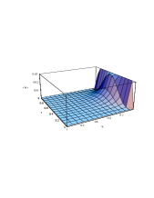
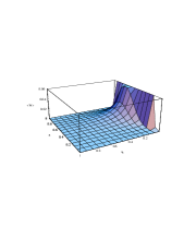
Figure 3: A three-dimensional view of the quantity $-\sum_{a,\bar{a}}e^{2}_{a}\Bigl{[}x_{B}h_{1L}^{\perp(1)a}(x_{B})\tilde{H}^{a}(z_{h})/z-x_{B}^{2}h_{L}^{a}(x_{B})H_{1}^{\perp(1)a}(z_{h})\Bigr{]}$, relevant for the $\sin(\phi^{l}_{h})$ asymmetry in $\pi^{+}$ production, as obtained under the approximation $\tilde{h}_{L}=\overline{h}_{L}=0$ (on the left) and under the approximation $h_{1L}^{\perp(1)}(x)=0$ (on the right).

Conclusions and future perspectives

Single spin asymmetries are an important tool to learn about distribution and fragmentation functions, and ultimately to study the spin content of nucleons. In fact, distribution and fragmentation functions tell us about the internal structure of the nucleons and of the role their elementary constituents play in accounting for their total spin. It is then crucial to study those processes in which these functions can be exploited. After many years of efforts, both on the experimental and theoretical point of view, experimental information on polarized distribution and fragmentation functions is now starting to come from different sources (HERMES, SMC, SLAC, COMPASS, RHIC and JLAB). Thus, some light can be shed, even though we are still far from a completely clear picture. This is another little step helping to draw a neater picture of the very intriguing “soft” physics which governs the hadronic world.

M. Boglione wishes to thank Mirek Finger for his invitation to such a nice and interesting conference. This research project was supported by the Foundation for Fundamental Research on Matter (FOM).

References

• [1] M. Boglione, E.Leader, hep-ph/0005092, to appear in the Proceedings of the HiX2000 Workshop, Philadelphia, March 30th-31st 2000, and on the Proceedings of ”Les Rencontres de Physique de la Valle d’Aoste”, Results and perspectives in particle physics, La Thuile, February 27- March 4 2000.
• [2] D.E. Soper, Phys. Rev. D 15, 1141 (1977); Phys. Rev. Lett. 43, 1847 (1979).
• [3] R.L. Jaffe, Nucl. Phys. B 229 (1983) 205.
• [4] M. Anselmino, M. Boglione, F. Murgia, Phys. Lett. B 362, (1995) 164; Phys. Rev. D 60, (1999) 054027.
• [5] D.L. Adams et al, Phys. Lett. B 261, 201 (1991) and Phys. Lett. B 264, 462 (1991).
• [6] M. Boglione and E. Leader, Phys. Rev. D 61, (2000) 114001.
• [7] D. Boer and P.J. Mulders, Phys. Rev. D 57, (1998) 5780.
• [8] M. Boglione, P.J. Mulders, Phys. Rev. D 60 (1999) 054007.
• [9] M. Boglione, P.J. Mulders, Phys. Lett. B 478 (2000) 114.
• [10] H. Avakian, contribution to the Proceedings of the 8th Workshop on Deep Inelastic Scattering, DIS00, Liverpool 25th-30th April, 2000.