Abstract

We obtain a class of solutions for the AdS₅ two-brane models by imposing the observed value of cosmological constant and Newton coupling constant on the visible brane. When all terms up to the first order of matter density are included, the cosmological evolution on the observable brane depends on the equation of state of the matter and consequently when the pressure exists, the cosmology of these models deviates from FLRW cosmology. We show that it is possible to choose the matter equation of state on the hidden brane to neutralize its contribution on the cosmological evolution of the visible brane. We compare the prediction of these models for primordial ⁴He yield with observations. In standard BBN with $n_{\nu}^{light}=3$ this brane model is ruled out. If in addition to $3$ SM neutrinos there is one light sterile neutrino, this model reconciles the observed ⁴He yield with a high ${\Omega}_{b}\sim 0.033h^{-2}$ suggested by BOOMERANG and MAXIMA experiments.

1 Introduction and Conclusions

Since early works on the cosmology of brane models [4] [5]  [6] it is well known that they don’t have a standard cosmology i.e. the evolution of Hubble constant on the observable brane depends on the matter density in place of its square root. Nonetheless, it has been argued [5] [2] that when the density of matter is much smaller than the absolute value of the brane tension, the effect is negligible and the matter part of $H^{2}$ evolution equation can be linearized. For RS-like models this condition is satisfied roughly from before BBN to today and should not have observable consequences on the light elements yield. Moreover, in the case of one-brane models, special choice of $\hat{T}^{55}$ can retrieve the standard FLRW evolution. These solutions are related to the stabilization mechanism of the branes [7]. Two-brane models have additional complexities and the matter density on the two branes are coupled. This can seriously influence the plausibility of these models.
In two recent works [1] and  [2] the solutions of two-brane models have been investigated. In  [1] only RS models [3] with one negative tension brane and one positive tension brane are considered. They satisfy the well known relation ${\rho}_{{\Lambda}_{L}}=-{\rho}_{{\Lambda}_{L}}=-{\rho}_{B}/\mu=6\mu/{\hat{\kappa}}^{2}$ (see below for definitions). In [2], Kanti et al.solve the evolution equations for a general case. They apply constraints on the hidden brane and their approximations lead to the same cosmological behavior on both branes.
Here we perform the same calculation as in [2] with the difference that we consider all relevant terms up to first order of the matter densities in the model. We show that in this case, even when the matter density is much smaller than the brane tension and the higher order terms are negligible, the cosmology on the observable brane deviates from FLRW one and depends on the matter equation of state on the brane. It is however possible to fine tune the equation of state on the hidden brane such that the cosmological evolution of branes decouples. By applying the observational constraints i.e. having a very small cosmological constant on the observable brane and the solution of the hierarchy problem, we find that at least for this subset of solutions, the smallness of the cosmological constant and warp factor ($N^{2}$ as defined below) are related. Moreover, the equation of state on the hidden brane becomes very close to the pure cosmological constant type.
The evolution equation however continues to depend on the pressure. We investigate the effect of this unconventional cosmology on the primordial nucleosynthesis. By comparing the prediction of these two-brane models for ⁴He yield with observation, we show that for a standard particle physics model with $n_{\nu}^{light}=3$ they lead to a too small primordial ⁴He. For $n_{\nu}^{light}=4$ e.g. if there is one strile neutrino, this class of brane models are compatible with the low ⁴He observation [8] and ${\eta}$ in the range predicted by BBN. For high baryon density observed by new CMB experiments BOOMERANG [9] and MAXIMA [10], it is compatible with the whole observationally acceptable range of ⁴He.

2 Solutions of Two 3-Brane Models

The start point of the model is the assumption of one extra dimension. Motivated by orbifold compactification of one of space dimensions in string theory on ${\bf S_{1}}/{\bf Z_{2}}$ [11], the positive and negative side of the fifth dimension are identified. Considering a homogeneous metric for other space dimensions, the metric is defined as:

$$ds^{2}=-n^{2}(t,y)dt^{2}+a^{2}(t,y)\delta_{ij}dx^{i}dx^{j}+b^{2}(t,y)dy^{2}.$$ (1)

The orbifoldized dimension is bounded by two 3-branes with coordinate separation $L$. If $L\rightarrow\infty$, one forgets the brane at infinity (i.e. regulator brane) and the brane at $y=0$ is identified with our 4-dim. Universe. The action of this model is defined as:

$$S=-\int d^{4}xdy\sqrt{(-\hat{g})}\biggl{(}\frac{\hat{R}}{2{\hat{\kappa}}^{2}}+{\Lambda}_{B}+{\Lambda}_{0}\delta(y)+{\Lambda}_{L}\delta(y-L)+\hat{\mathcal{L}}_{m}\biggr{)}.$$ (2)

Hatted quantities are in 5-dimensional space. The Einstein equations becomes:

$$\hat{G}_{00} = 3\biggl{\{}\frac{\dot{a}}{a}\biggl{(}\frac{\dot{a}}{a}+\frac{\dot{b}}{b}\biggr{)}-\frac{n^{2}}{b^{2}}\biggl{[}\frac{a^{\prime\prime}}{a}+\frac{a^{\prime}}{a}\biggl{(}\frac{a^{\prime}}{a}+\frac{b^{\prime}}{b}\biggr{)}\biggr{]}\biggr{\}}={\hat{\kappa}}^{2}\hat{T}_{00},$$ (3)

$$\hat{G}_{ij} = \frac{a^{2}}{b^{2}}\biggl{\{}\frac{a^{\prime}}{a}\biggl{(}\frac{a^{\prime}}{a}+2\frac{n^{\prime}}{n}\biggr{)}-\frac{b^{\prime}}{b}\biggl{(}\frac{n^{\prime}}{n}+2\frac{a^{\prime}}{a}\biggr{)}+2\frac{a^{\prime\prime}}{a}+\frac{n^{\prime\prime}}{n}\biggr{\}}$$ (4)

$$+ \frac{a^{2}}{n^{2}}\biggl{\{}\frac{\dot{a}}{a}\biggl{(}-\frac{\dot{a}}{a}+2\frac{\dot{n}}{n}\biggr{)}-2\frac{\ddot{a}}{a}+\frac{\dot{b}}{b}\biggl{(}-2\frac{\dot{a}}{a}+\frac{\dot{n}}{n}\biggr{)}-\frac{\ddot{b}}{b}\biggr{\}}={\hat{\kappa}}^{2}\hat{T}_{ii},$$

$$\hat{G}_{05} = 3\biggl{(}\frac{n^{\prime}\dot{a}}{na}+\frac{a^{\prime}\dot{b}}{ab}-\frac{\dot{a^{\prime}}}{a}\biggr{)}=0,$$ (5)

$$\hat{G}_{55} = 3\biggl{\{}\frac{a^{\prime}}{a}\biggl{(}\frac{a^{\prime}}{a}+\frac{n^{\prime}}{n}\biggr{)}-\frac{b^{2}}{n^{2}}\biggl{[}\frac{\dot{a}}{a}\biggl{(}\frac{\dot{a}}{a}-\frac{\dot{n}}{n}+\frac{\ddot{a}}{a}\biggr{)}\biggr{]}\biggr{\}}={\hat{\kappa}}^{2}\hat{T}_{55}.$$ (6)

The parameter $\hat{\kappa}^{2}=8\pi/M^{3}_{5}$ is the gravity coupling constant and $\hat{T}_{AB},\quad A,B={0,\ldots,3\&5}$ is the energy-momentum tensor in 5-dim. space-time. We define $\hat{T}^{A}_{B}=\hat{T}^{A}_{bulkB}+\hat{T}^{A}_{0B}+\hat{T}^{A}_{LB}$ as the following:

$$\hat{T}^{A}_{bulkB} = diag(-{\rho}_{B},P_{B},P_{B},P_{B},\hat{T}^{5}_{5}),$$ (7)

$$\hat{T}^{A}_{0B} = \frac{\delta(y)}{b}diag(-{\rho}_{0},P_{0},P_{0},P_{0},0),$$ (8)

$$\hat{T}^{A}_{LB} = \frac{\delta(y-L)}{b}diag(-{\rho}_{L},P_{L},P_{L},P_{L},0).$$ (9)

${\rho}_{i}={\rho}_{m_{i}}+{\rho}_{{\Lambda}_{i}}$, $P_{i}=P_{m_{i}}-{\rho}_{{\Lambda}_{i}}$, $i$ = $0$ or $L$. It is assumed that they satisfy Bianchi identities:

$$\dot{{\rho}}_{B}+3\frac{\dot{a}}{a}({\rho}_{B}+P_{B})+\frac{\dot{b}}{b}({\rho}_{B}+\hat{T}^{5}_{5}),$$ (10)

$$\hat{T^{\prime}}^{5}_{5}+3\frac{a^{\prime}}{a}(\hat{T}^{5}_{5}-P_{B})+\frac{n^{\prime}}{n}({\rho}_{B}+\hat{T}^{5}_{5}).$$ (11)

The restriction of (10) to branes includes $\dot{b}$ i.e. the expansion of the bulk contributes to the density conservation on the brane. This would change the evolution of the observable Universe and contradict observations. Therefore, we assume that $b$ and the distance between branes has been stabilized [12] at a very early time and after inflation they are time independent. In this case $b$ can be redefine such that it become a constant and normalized to $b=1$.
The discontinuity of $a^{\prime}$ and $n^{\prime}$ on the branes leads to the following boundary conditions:

$$\frac{[a^{\prime}]_{0}}{a_{0}b}=-\frac{{\hat{\kappa}}^{2}}{3}{\rho}_{0}, \frac{[a^{\prime}]_{L}}{a_{L}b}=\frac{{\hat{\kappa}}^{2}}{3}{\rho}_{L}.$$ (12)

$$\frac{[n^{\prime}]_{0}}{n_{0}b}=\frac{{\hat{\kappa}}^{2}}{3}(2{\rho}_{0}+3P_{0}), \frac{[n^{\prime}]_{L}}{n_{L}b}=-\frac{{\hat{\kappa}}^{2}}{3}(2{\rho}_{L}+3P_{L}).$$ (13)

where $[A]_{x}=A_{x^{+}}-A_{x^{-}}$. It is easy to verify that conditions (13) are satisfied once (12) and energy-momentum conservation on the branes (restriction of (10)) are satisfied.
From equation (5):

$$n(t,y)=\frac{\dot{a}(t,y)}{\alpha(t)}.$$ (14)

where $\alpha(t)$ is an arbitrary function of $t$. Choosing $n(t,0)=1$, i.e. synchronous gauge on the $y=0$ brane, $\alpha(t)=\dot{a}_{0}(t)$.
We assume that ${\rho}_{B}$ and $P_{B}$ don’t depend on $y$. In this case (10) is true only if these quantities are also time independent i.e. has the form of a cosmological constant. With this energy-momentum tensor, (3) and (6) give the evolution equation of $a(t,y)$ [4]:

$$(aa^{\prime})^{\prime}-{\alpha}^{2}(t)=\frac{a^{2}{\hat{\kappa}}^{2}T^{0}_{0}}{3}.$$ (15)

For ${\rho}_{B}<0$, equation (15) has the following solution:

$$a^{2}(t,y)=A(t)\cosh(\mu y)+B(t)\sinh(\mu y)+C(t).\quad\quad\mu=\sqrt{\frac{2{\hat{\kappa}}^{2}}{3}|{\rho|}_{B}}.$$ (16)

Comparing $y$ independent part of (16) and (3) gives:

$$C(t)=\frac{3{\alpha}^{2}}{{\hat{\kappa}}^{2}{\rho}_{B}}.$$ (17)

$A$ and $B$ are determined from (12) and (13):

$$A(t)=a^{2}_{0}-c(t),\quad\quad\quad B(t)=-\frac{{\hat{\kappa}}^{2}}{3\mu}{\rho}_{0}a^{2}_{0}.$$ (18)

Evaluating (12) for $L$-brane using (16) leads to:

$$\frac{{\alpha}^{2}(t)}{a_{0}^{2}}=\frac{{\dot{a}}_{0}^{2}}{a_{0}^{2}}=\frac{{\hat{\kappa}}^{2}{\rho}_{B}}{3}\biggl{[}\frac{({\rho}^{\prime}_{0}{\rho}^{\prime}_{L}+1)\sinh(\mu L)-({\rho}^{\prime}_{0}+{\rho}^{\prime}_{L})\cosh(\mu L)}{{\rho}^{\prime}_{L}(1-\cosh(\mu L))+\sinh(\mu L)}\biggr{]}$$ (19)

For any density $\rho$, ${\rho}^{\prime}\equiv\frac{\rho}{{\Lambda}_{RS}}$, ${\Lambda}_{RS}\equiv\frac{3\mu}{{\hat{\kappa}}^{2}}$. From (16), (17) and (18):

$$\frac{a_{L}^{2}(t)}{a_{0}^{2}(t)}=\frac{{\rho}^{\prime}_{0}(1-\cosh(\mu L)+\sinh(\mu L))}{{\rho}^{\prime}_{L}(1-\cosh(\mu L))+\sinh(\mu L)}$$ (20)

By differentiating (20) and using (19), the evolution equation on the visible brane and relation between warp factors can be determined:

$$\frac{{\dot{a}}_{L}^{2}}{a_{L}^{2}} = \frac{{\hat{\kappa}}^{2}{\rho}_{B}}{3}\biggl{[}\frac{({\rho}^{\prime}_{0}{\rho}^{\prime}_{L}+1)\sinh(\mu L)-({\rho}^{\prime}_{0}+{\rho}^{\prime}_{L})\cosh(\mu L)}{({\rho}^{\prime}_{0}(1-\cosh(\mu L))+\sinh(\mu L))^{2}}\biggr{]}$$

$$\biggl{[}\frac{(2{\rho}^{\prime}_{{\Lambda}_{0}}-{\rho}^{\prime}_{m_{0}}-3P^{\prime}_{m_{0}})(1-\cosh(\mu L))+2\sinh(\mu L)}{(2{\rho}^{\prime}_{{\Lambda}_{L}}-{\rho}^{\prime}_{m_{L}}-3P^{\prime}_{m_{L}})(1-\cosh(\mu L))+2\sinh(\mu L)}\biggr{]}^{2}({\rho}^{\prime}_{L}(1-\cosh(\mu L))+\sinh(\mu L))$$

$$\frac{n_{L}^{2}}{n_{0}^{2}} = \frac{a^{2}_{0}}{a^{2}_{L}}\biggl{[}\frac{(2{\rho}^{\prime}_{{\Lambda}_{0}}-{\rho}^{\prime}_{m_{0}}-3P^{\prime}_{m_{0}})(1-\cosh(\mu L))+2\sinh(\mu L)}{(2{\rho}^{\prime}_{{\Lambda}_{L}}-{\rho}^{\prime}_{m_{L}}-3P^{\prime}_{m_{L}})(1-\cosh(\mu L))+2\sinh(\mu L)}\biggr{]}^{2}$$ (22)

With supplementary assumption ${\rho}^{\prime}_{{\Lambda}_{i}}\gg{\rho}^{\prime}_{m_{i}}$, after expansion to first order of matter density, the evolution equation (LABEL:adotl2) becomes:

$$\frac{{\dot{a}}_{L}^{2}}{a_{L}^{2}} = \frac{{\hat{\kappa}}^{2}{\rho}_{B}{\mathcal{A}}}{3{\mathcal{C}}}\biggl{[}1+\biggl{(}\frac{{\rho}^{\prime}_{{\Lambda}_{0}}\sinh(\mu L)-\cosh(\mu L)}{{\mathcal{A}}}+\frac{2(1-\cosh(\mu L))}{{\mathcal{C}}}\biggr{)}{\rho}^{\prime}_{m_{L}}+$$ (23)

$$\biggl{(}\frac{{\rho}^{\prime}_{{\Lambda}_{L}}\sinh(\mu L)-\cosh(\mu L)}{{\mathcal{A}}}-\frac{3(1-\cosh(\mu L))}{{\mathcal{B}}}\biggr{)}{\rho}^{\prime}_{m_{0}}+$$

$$\frac{3(1-\cosh(\mu L))}{{\mathcal{C}}}P^{\prime}_{m_{L}}-\frac{3(1-\cosh(\mu L))}{{\mathcal{B}}}P^{\prime}_{m_{0}}+{\mathcal{O}}({\rho^{\prime}}_{m}^{2})\biggr{]}$$

$${\mathcal{A}} \equiv ({\rho}^{\prime}_{{\Lambda}_{0}}{\rho}^{\prime}_{{\Lambda}_{L}}+1)\sinh(\mu L)-({\rho}^{\prime}_{{\Lambda}_{0}}+{\rho}^{\prime}_{{\Lambda}_{L}})\cosh(\mu L)$$ (24)

$${\mathcal{B}} \equiv {\rho}^{\prime}_{{\Lambda}_{0}}(1-\cosh(\mu L))+\sinh(\mu L)$$ (25)

$${\mathcal{C}} \equiv {\rho}^{\prime}_{{\Lambda}_{L}}(1-\cosh(\mu L))+\sinh(\mu L)$$ (26)

As noticed in  [1] and  [2], the evolution equation on visible brane depends on the matter on both branes. Here we see that considering the full expansion of (LABEL:adotl2) to first order, not only the evolution depends on the matter on both branes but also on their equation of state even at late time (In  [6] the same dependence has been obtained for one brane models before stabilization). It is in strict conflict with the evolution of FLRW metric which only depends on the matter density. It is easy to verify that for large $\mu L$, the amplitudes of density and pressure terms are comparable and it is not possible to neglect the pressure term. This behavior has important consequences for nucleosynthesis in the early universe. We address this issue in the next section.
Equation (23) has also another interesting consequence. It is possible to fine-tune the equation of state of the matter on the hidden brane such that it decouples from the cosmological evolution of the visible brane. Assuming $P_{i}=w_{i}{\rho}_{i}$, $i=0$ or $L$ as the equation of state for matter and ${\gamma}_{0}\equiv 1+w_{0}$ and ${\gamma}^{\prime}_{L}\equiv\frac{2}{3}+w_{L}$, the value of ${\gamma}_{0}$ which eliminates the contribution of the matter on the hidden brane from (23) is:

$${\gamma}_{0}=\frac{{\mathcal{B}}({\rho}^{\prime}_{{\Lambda}_{L}}\sinh(\mu L)-\cosh(\mu L))}{3{\mathcal{A}}(1-\cosh(\mu L))}$$ (27)

Our numerical calculation shows that for the interesting range of the only parameter of the model i.e. $5<\mu L<50$, the value of $w_{0}$ from (27) is very close to $-1$. This means that if this model corresponds to real universe, matter can be absent from the hidden brane or it can be a scalar field with a quintessential behavior. It would be interesting to see if stabilization models can predict such partition of matter between branes.
In the next step we use the linearized equation (23) to identify observable quantities like cosmological constant and Newton coupling constant. The visible brane must have an evolution equation similar to FLRW cosmology. We parameterize (23) as the following:

$$\frac{{\dot{a}}_{L}^{2}}{a_{L}^{2}}=\frac{8\pi G}{3}(\alpha{\rho}_{m_{obs}}+{\rho}_{{\Lambda}_{obs}}+{\mathcal{O}}({\rho}_{m}^{2})).$$ (28)

Quantities ${\rho}_{m_{obs}}$ and ${\rho}_{{\Lambda}_{obs}}$ are respectively observed matter density of the Universe and observed cosmological constant; $\alpha$ is a dimensionless quantity. For FLRW cosmology $\alpha=1$. For brane models in general $\alpha$ can depend on $\mu L$ and the equation of state.
In  [2] constraints are imposed on the hidden brane. In fact in that work, the square term in (LABEL:adotl2) is neglected and the evolution equations on both branes have the same form and there is no difference on which brane constraints are imposed. Here we apply them on the visible brane. When (27) is satisfied, the value of three unknown parameters ${\Lambda}_{RS}$, ${\rho}^{\prime}_{{\Lambda}_{0}}$ and ${\rho}^{\prime}_{{\Lambda}_{L}}$ can be fixed by comparing (28) and (23) and an additional condition on the warp factor [2] [13]:

$${\rho}_{{\Lambda}_{obs}} = \frac{{\hat{\kappa}}^{2}{\rho}_{B}}{8\pi G}\biggl{[}\frac{{\mathcal{A}}}{{\mathcal{C}}}\biggr{]}$$ (29)

$$8\pi G = \frac{{\hat{\kappa}}^{2}{\rho}_{B}}{{\Lambda}_{RS}}\biggl{[}\frac{({\rho}^{\prime}_{{\Lambda}_{0}}\sinh(\mu L)-\cosh(\mu L)){\mathcal{C}}+2(1-\cosh(\mu L)){\mathcal{A}}}{{\mathcal{C}}^{2}}\biggr{]}$$ (30)

$$N^{2} \equiv \frac{M^{2}_{5}}{M^{2}_{pl}}=\frac{n^{2}_{L}}{n^{2}_{0}}=\frac{{\mathcal{B}}}{{\mathcal{C}}}$$ (31)

Note that only the value of $\alpha G$ can be determined from (28) and (23). Here we define $G$ such that:

$$\alpha=1+\beta w_{L}$$ (32)

and $\beta$ depends only on $\mu L$ and not on the matter density:

$$\beta=\frac{3{\mathcal{A}N^{2}}(1-\cosh(\mu L))}{{\mathcal{B}}\biggl{(}{\rho}^{\prime}_{{\Lambda}_{L}}\sinh(\mu L)-\cosh(\mu L)\biggr{)}-3{\mathcal{A}}\biggl{(}1-\cosh(\mu L)\biggr{)}}$$ (33)

The equation (31) is obtained after neglecting time dependent terms. By applying the same procedure on the quantities of the hidden brane, one finds that:

$$G^{\prime}=\frac{G}{N^{2}}\biggl{(}1-\frac{3{\gamma}^{\prime}(1-\cosh(\mu L)){\rho}^{\prime}_{{\Lambda}_{obs}}}{{\mathcal{C}}^{2}}\biggr{)}$$ (34)

where $G^{\prime}$ is the Newton coupling constant on the hidden brane. According to (34) the gravitational coupling on the hidden brane is much stronger than on the observable one.
From equations (29) to (31) one obtains a $5^{th}$ order equation for ${\Lambda}_{RS}$. Due to presence of very large and very small parameters (respectively $\cosh(\mu L)$, $N^{2}$ and ${\rho}_{obs}/J$ (see (35) below for the definition of J)), in this equation, one must be very careful about approximations because the combination of large and small parameters can lead to quantities which are not negligible. For $\cosh(\mu L)\gg 1$ and $N^{2}\cosh(\mu L)\ll 1$, a simple analytical solution for ${\Lambda}_{RS}$ can be found:

$${\Lambda}_{RS}=J\biggl{(}\frac{3{\gamma}^{\prime}_{L}{\rho}^{2}_{{\Lambda}_{obs}}{\cosh}^{2}(\mu L)}{N^{2}J^{2}}\biggr{)}^{\frac{1}{3}}\cosh(\mu L)\quad\quad\quad J\equiv\frac{48\pi G}{{\hat{\kappa}}^{4}}$$ (35)

It is valid only for $M_{5}\gtrsim 10^{14}eV$. Figs. 1 and 2 show ${\Lambda}_{RS}$, ${\rho}^{\prime}_{{\Lambda}_{0}}$, ${\rho}^{\prime}_{{\Lambda}_{L}}$ as a function of $\mu L$. It is interesting to note that in this approximative solution, the smallness of the observed cosmological constant and $N^{2}$ are related. In fact according to this solution, the value of ${\rho}^{2}_{{\Lambda}_{obs}}$ and $N^{2}$ must be roughly of the same order to not have too small or too large ${\Lambda}_{RS}$ (for fixed $J$ and $\mu L$). It is also evident that in this approximation an exactly null cosmological constant is not acceptable because ${\Lambda}_{RS}$ would be zero too.
Another aspect of this solution is the positiveness of tension on both branes. Using (29) to (31), it is not difficult to see that when $\mu L$ is large, tensions are both very close to ${\Lambda}_{RS}$ (this has been also observed in  [2]). A difference of order $\cosh^{-1}(\mu L)$ between normalized tensions assures the small warp factor Eq. (31).

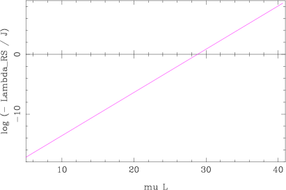
Figure 1: Approximative solution of ${\Lambda}_{RS}$ for $M_{5}=10^{15}eV$.

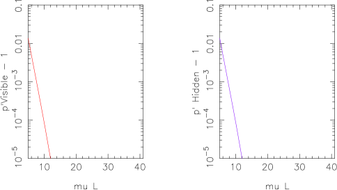
Figure 2: ${\rho}^{\prime}_{0}$ and ${\rho}^{\prime}_{L}$ from the approximative solution (35) for $M_{5}=10^{15}eV$.

3 Primordial Nucleosynthesis

In the previous section we have seen that when the matter pressure is not negligible, the cosmology of two-brane models deviates from the FLRW cosmology even if the higher order terms are negligible. It is therefore necessary to determine the prediction of this class of brane models for the Big Bang Nucleosynthesis and the yield of the light elements.
In a brane universe with cold and hot matter on the visible brane, the evolution equation of the visible brane (28) can be written as:

$$H^{2}\equiv\frac{{\dot{a}}_{L}^{2}}{a_{L}^{2}}=\frac{8\pi G}{3}({\alpha}_{hot}{\rho}_{hot}+{\rho}_{cold}+{\rho}_{{\Lambda}_{obs}}+{\mathcal{O}}({\rho}_{m}^{2})).$$ (36)

At the time of nucleosynthesis the contribution of higher order terms, cold component and cosmological constant are negligible and:

$$H^{2}=\frac{8\pi G}{3}{\alpha}_{hot}{\Omega}_{hot}(1+z)^{4}$$ (37)

where $z$ is the redshift. Equation (37) has the same form as FLRW cosmology with an effective mass of ${\alpha}_{hot}{\Omega}_{hot}$.
The relation between primordial yield of light elements depends on the temperature of the $p-n$ plasma when neutrinos decouple from weak interaction $p+e\leftrightarrows n+\nu$ (see e.g.  [14]). In the unconventional cosmology of (37):

$$\frac{{\Gamma}_{pe\leftrightarrows n\nu}}{H}\approx\frac{1}{{\alpha}^{\frac{1}{2}}}\biggl{(}\frac{T}{0.8MeV}\biggr{)}^{3}$$ (38)

Or in another word $T_{freez-out,brane}\equiv T_{F}\sim{\alpha}^{\frac{1}{6}}0.8MeV$. With this new freeze-out temperature, the neutron-to-proton ratio becomes:

$$\biggl{(}\frac{n}{p}\biggr{)}_{freeze-out,brane}=\exp\biggl{(}-\frac{Q}{T_{F}}\biggr{)}=\biggl{(}\frac{n}{p}\biggr{)}^{{\alpha}^{-\frac{1}{6}}}_{freeze-out,FLRW}$$ (39)

When $\mu L\gg 1$ and ${\rho}_{0}\approx{\rho}_{L}$, using (32) and (33), $\alpha\approx\frac{2}{3}$. Assuming

$$\biggl{(}\frac{n}{p}\biggr{)}_{freeze-out,FLRW}\approx\frac{1}{7}=0.143$$ (40)

results to:

$$\biggl{(}\frac{n}{p}\biggr{)}_{freeze-out,brane}\approx 0.125$$ (41)

i.e. the prediction of the two-brane model studied in the previous section is $\sim 12\%$ less than standard cosmology. Fig.3 shows the ⁴He yield $Y_{p}$ as a function of $\eta\equiv n_{b}/n_{\gamma}$ for FLRW and for the two-brane models and compares them with observations. It is evident that for $n^{light}_{\nu}=3$ the brane model is ruled out for all reasonable values of $\eta$. However, the observation of neutrino oscillation by Super-Kamiokand experiment and others [15] joint with the results of LSAND experiment [16] strongly suggests the existence of a sterile neutrino mixing with the SM neutrinos. In this case the number of light neutrinos is larger than $3$. Fig.3 shows also the ⁴He yield for $n^{light}_{\nu}=4$ for FLRW and the two-brane models. The latter is compatible with the observation specially if ${\Omega}_{b}$ or equivalently $\eta$ is as large as what is suggested by BOOMERANG [9] and MAXIMA [10] experiments. In fact the SBBN has difficulties to reconcile ${\Omega}_{b}$ ($\eta$) obtained from these experiments with the independent measurement of ⁴He [8] [18] and deuterium [19] yields. It is possible to reconcile ⁴He and CMB observations in the standard cosmology if there is a sterile neutrino and an initial lepton asymmetry [17]. However, to have an effective number of neutrinos less than $3$, the sterile neutrino must be the lightest one and the mass difference between ${\nu}_{s}$ and ${\nu}_{e}$ must be $\delta m^{2}\lesssim 1eV^{2}$ [17]. Two-brane models by contrast are less sensitive to the parameter space of neutrinos and don’t need an initial lepton asymmetry.
None of FLRW or brane models however can reconcile the observed value of ${}^{2}D$ if ${\Omega}_{b}\gtrsim 0.03h^{-2}$. An entropy increase after BBN has been suggested to reconcile two observations [20]. In this case, according to Fig.3 the brane model would be only compatible with a low ⁴He yield if $\eta$ has a value in the range predicted by SBBN.
Conclusions of this section are not very sensitive to the details of the two-brane model. The asymptotic value of $\beta$ is valid for a large range of parameters $M_{5}$ and $\mu L$. We have restricted the analysis to the special model with decoupled branes. In the general case the conclusion depends on the density and pressure on the hidden brane which are not directly observable.

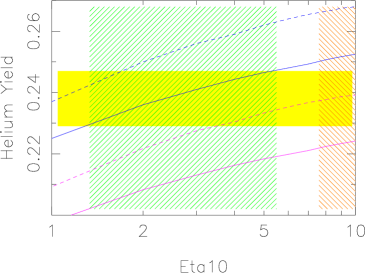
Figure 3: Primordial Helium yield: FLRW (blue), model explained in Spec. $2$ (magenta). Full and dashed curves correspond respectively to $n^{light}_{\nu}=3$ and $n^{light}_{\nu}=4$. The hashed regions show a conservative range for the observed value of $Y_{p}$ (yellow) and corresponding ${\eta}_{10}$ according to BBN (light green) and new value of ${\eta}_{10}$ from CMB anisotropy observation (red).

References

- [1] Lesgourgues J., Pastor S., Peloso M. & Sorbo L., Phys. Lett. B 489, 411 (2000), hep-ph/0004086.
- [2] Kanti P., Olive K.A. & Pospelov M., hep-ph/0005146.
- [3] L. Randall & R. Sundrum, Phys. Rev. Lett. 83, 3370 (1999), hep-ph/9905221; Phys. Rev. Lett. 83, 4690 (1999), hep-ph/9906064.
- [4] Binétury P., Deffayet C. & Langlois D., Nucl. Phys. B 565, 269 (2000), hep-th/9905012; Phys. Lett. B 477, 285 (2000), hep-th/9910219.
- [5] Lukas A., Ovrut, b.A., Stelle K.S. & Waldram D., Phys. Rev. D 59, 086001 (1999), Lukas A., Ovrut, b.A. & Waldram D., Phys. Rev. D 61, 023506 (2000), Mohapatra R.N., Pérez-Lorenzana A.& de S. Pires C.A., peh-ph/0003328.
- [6] Flanagan E., Tye S.H.H. & Wasserman I., hep-ph/9910498.
- [7] Kanti P., Kogan I.I., Olive K.A. & Pospelov M., Phys. Lett. B 468, 31 (1999), hep-ph/9909481, Phys. Rev. D 61, 106004 (2000), hep-ph/9912266; Csáki C. et al., Phys. Rev. D 62, 045015 (2000), hep-ph/9911406.
- [8] Olive K.A., Skillman E.D. & Steigman G ApJ. 483, 788 (1997), astro-ph/9611166.
- [9] Lange A.E. et al., astro-ph/0005004.
- [10] Balbi A. et al., astro-ph/0005124.
- [11] Horava P. & Witten E.,Nucl. Phys. B 460, 506 (1996), hep-th/9507060, Nucl. Phys. B 475, 94 (1996), hep-th/9603142; Witten E. Nucl. Phys. B 471, 135 (1996), hep-th/9602070.
- [12] Goldberger W.D & Wise M.B., Phys. Rev. Lett. 83, 4922 (1999), hep-ph/9907447.
- [13] N. Arkani-Hamed, Dimopoulos & G. Dvali, Phys. Lett. B 429, 263 (1998), hep-ph/9807344; I. Antoniadis, et al., PLB 436, 257 (1998), hep-ph/9804398.
- [14] Kolbe E. & Turner M., ”The Early Universe”, Addison Wesley Pub. Co. (1990).
- [15] Fukuda Y. et al., Phys. Lett. B 335, 237 (1994); Becker-Szendyet R. et al.Nucl. Phys. B 38, 331 (1995)(Proc. Supp.); Allison W.M. et al., Phys. Lett. B 391, 491 (1997), hep-ex/9611007; Ambrosio M. et al., Phys. Lett. B 434, 451 (1998), hep-ex/9807005; Fukuda Y. et al., Phys. Rev. Lett. 81, 1562 (1998), hep-ex/9807003.
- [16] Athanassopoulos C. et al., Phys. Rev. Lett. 77, 3082 (1996), nucl-ex/9605003; Phys. Rev. Lett. 81, 1774 (1998), nucl-ex/9709006.
- [17] Di Bari P. & Foot R. astro-ph/0008258 and references therein.
- [18] Izotov Y.L. & Thuan T.X., ApJ. 500, 188 (1998), astro-ph/9811387.
- [19] Rugers M. & Hogan C.J., Astro. J. 111, 2135 (1996), astro-ph/9603084; Burles S. & Tytler D., ApJ. 499, 699 (1998), ApJ. 507, 732 (1998).
- [20] Kaplinghat M & Turner M., astro-ph/0007454.