The scalar field-theoretical Coulomb problem

Abstract

We analyze the fully relativistic, field-theoretical treatment of the scalar Coulomb problem. We work in a truncated Hilbert-Fock space containing the two-constituent states and the two-constituent-and-one-massless-exchange-particle states. Self-energy contributions are dominant for large values of the coupling constant. Using the covariant formulation of the self-energy does not alter these results significantly. Both the weak-coupling limit and the heavy-mass limit lead to the non-relativistic results.

1 Introduction

In this paper we will solve the simplest possible scalar field-theoretical Coulomb problem in a Hamiltonian framework [1]. This approach is much simpler than most other field-theoretical approaches, and yields better results. Furthermore, we also include the self-energy parts, which are usually ignored, and find that they give significant contributions. Our main motivation for this work lies in improving our understanding of the field-theoretical bound-state problem before we turn our attention to stronger binding, and more physical, cases.

There is a wealth of relativistic bound-state equations [2, 3, 4]. Most of them are three-dimensional reductions of the Bethe-Salpeter equation [5] in the ladder approximation. Since there is a degree of arbitrariness involved in this reduction [6, 7], the equations can be tailored to satisfy unitarity [3], gauge invariance [8], or the one-body limit [6], which are some of the typical problems with the underlying Bethe-Salpeter equation [9, 10]. However, these are approximations upon an equation with problems, which is a questionable practice.

Generally, it is difficult to favour one equation above the other [11]. Therefore, there has been some attempt to establish standard results [12, 7], which include all orders in perturbation theory, in the quenched approximation. To do so one starts from the path integral for the two-particles four-point function and integrate out some degrees of freedom analytically, and the resulting integral is integrated numerically in the Feynman-Schwinger representation by the Monte Carlo method. The typical problems with this method are related to the discretisation of space-time, the Wick rotation, which leads to decaying states of which only the lowest-energy states can be determined accurately, and the problem to handle massless particles satisfactorily [7]. However, the results are promising and show the underbinding of the Bethe-Salpeter equation in the ladder approximation [13, 14].

Another, distinct approach is based on Haag’s expansion of asymptotic states in field theory in free and bound states, which lead to an hierarchy of coupled equations in the coupling constant expansion [15]. With some difficulty the scalar field theory, which is also analyzed here, is solved. The results seem to indicate a failure to obtain both the one-body limit and the weak-coupling limit in the Haag-expansion approach.

Most prominently has been the return to Hamiltonian field theory [1]. Because the bound-state is a stationary state, and manifest covariance is lost, it seems appropriate to solve the bound-state problem in the Hamiltonian framework. Most calculations are done in the light-front Hamiltonian framework [16, 17], which preserves part of the boost symmetry at the cost of rotational symmetry [18]. We will use the ordinary instant-form Hamiltonian instead to show that that indeed yields the same results as the Kepler problem [19], in the weak-coupling limit.

The reason to study the case of massless exchange particles in particular are manifold. Firstly, the massless particles are a typical and hard problem for field theory, as they generate long-range interactions, and lead to singularities in the S-matrix associated with multiple soft-photon emissions [20, 21]. None of these problems have to be present in the bound-state calculation. Indeed, in the Hamiltonian approach the infrared singularity is absent, contrary to the nonrelativistic treatment using the Coulomb potential and the covariant approach. When constituents are bound, they are off-shell, which means they do not share enough energy among them to become on-shell. Therefore they do certainly not have enough energy to radiate off soft photons, which is the origin of the infrared complications in the covariant approach [20, 22].

Consider the $S$-matrix element of two constituents exchanging a massless particle. This matrix element has a singularity. It occurs because at zero momentum exchange the difference in energy of the initial and intermediate states vanishes. If the two constituents belong to a bound state, the singularity is hidden by the binding energy. Apparently, the binding energy has the same effect as the mass of the exchanged particle: screening at long distances.

Secondly, eventually, one has to admit that all fundamental interactions that generate bound states are massless, gauge theories. For the case of positronium, a relativistic approach can be used [23], however, rather in the cumbersome Coulomb gauge [24] where the lowest-order kernel reduces to an instantaneous interaction, and many other cancellations occur. For the heavy-light case, like the hydrogen atom, the starting point has to be the non-relativistic Coulomb potential [25], or the equivalent Dirac equation with such a potential. This Coulomb potential has survived many revolutions in physics, mainly because of its phenomenological success: it predicts atomic spectra to a high accuracy [26, 25]. This success stood in the way of fundamental development, where the classical action-on-a-distance concept is replaced by the correct notion of particle exchange [5, 27]. There is no viable alternative which reproduces the particular long-range interaction generated by the exchange of massless particles. At least, there is no alternative that does not introduce additional problems in the one-body limit.

In this paper we recover the typical scaling associated with the weak-coupling Coulomb ground state. This paper is not just a formal exercise to link theory with experiment. Eventually, we like to understand how relativistic effects come about in deeply bound systems, and give sensible answers to where the spin of a system is coming from, how the radius of the bound state is related to the masses and the coupling strength, what the mass of a constituent is, and which are the effective degrees of freedom. We emphasize deeply bound states, i.e., states with a binding energy of the same order as the masses of the constituents, because we feel that for them the problems we want to address are most pressing. For weakly bound states one can treat relativistic aspects, like relativistic kinematics and the creation and annihilation of particles as a correction to the classical approach, where a potential picture is appropriate. Although it would be nice to understand better the origin and limitations of the potential picture.

The Hamiltonian framework is conceptually quite different from the standard, covariant field-theoretical framework, although the final formulae may be similar. In this framework exchange diagrams exist, but not as a potential. Rather, they are to be interpreted as matrix elements of the fundamental, local interactions, between different Fock sectors.

In the fundamental description of bound states there is no place for the concept of a potential. All interactions are local. What seems to be a non-local interaction is due to the smearing of the constituent particles, which are not just single particles but a linear combination of states with different numbers of bare particles.

The Hamiltonian description gives us a consistent way to truncate the infinite complexity arising in field theory, by truncating Fock space to two- and three-particle states. Many arguments concerning bound-states are devoted to the truncation to a finite number of particles, since, in order to generate a bound state which arises only non-perturbatively, an infinite summation of diagrams is required. So the question is which finite set one should take to iterate infinitely many times. For the Bethe-Salpeter equation [5] the results depend crucially on the answer to that question. However, formulated as a Hamiltonian eigenvalue problem this infinite summation appears naturally, given the Fock-state truncation. If this truncation to the two- and three-particle Fock-state sector is legitimate anywhere, it should be here, because in the weak-coupling limit a few particles are expected to contribute and anti-particles (Z-diagrams, which appear in a covariant approach) are expected to be suppressed, due to their large virtuality. We shall analyze the validity of these arguments.

So, for our problem we assume that our bound state consists of two pieces: one with two oppositely charged scalar particles and one with an additional, massless scalar particle that can be emitted and absorbed by each of the charged particles. We use scalar particles to keep the problem as simple as possible, and free from questions associated with gauge symmetry. A careful analysis of the three-particle state is required in order to recover all of the physics. One finds an exchange contribution and a self-energy contribution; the latter is infinite and has to be renormalized [28]. Of course, we face the problem of the interpretation of divergent integrals.

The concept of self-energy is still a mystery to many. In solid-state physics one can accept that a moving electron deforms the crystal, generating a drag which can be interpreted as an effective mass. In deep-inelastic scattering one can interpret the self-energy as the mixing-in of multi-particle states as sufficient energy becomes available when the particle goes off-shell. In a bound state the missing energy is the binding energy, which does not belong to a particular particle, but affects each of the particles separately. One may look upon this in the following way: each constituent is not a single particle; partly it is one particle, partly it is two, and so on. The relative weight of each of these states of a constituent is determined by two things: the number of states available and the virtuality of these states $\omega_{i}$. In a classical world only the one-particle state $\omega_{0}$ would exists because that state has the lowest energy $\omega_{0}<\omega_{i}$. In the quantum world and within the Hamiltonian framework, energy is only conserved asymptotically, so higher energy states, when available, will also be occupied. The weights of virtual states is determined by their virtualities. If we now put a “compound” constituent in a bound state with binding energy $E_{b}$, the relative virtuality $\omega_{i}/\omega_{0}>(\omega_{i}+E_{b})/(\omega_{0}+E_{b})$ of the multi-particle states in the constituent is less than for the free particle, therefore the summed energy will lower, and the self-energy will increase the binding.

2 Theory

In the present paper we solve the scalar Coulomb problem. We limit ourselves to this case in order to avoid numerous problems concerning gauge theories. Here we are rather interested in the conceptual problem of what a bound state is and what determines its properties in the simplest possible case. Spin effects and questions concerning gauge invariance can be dealt with later.

Our model Lagrangian describes the interaction of three scalar fields $\phi_{a}$, $\phi_{b}$, and $\chi$,

$${\cal L}=-\frac{1}{2}\psi_{a}[\partial^{\mu}\partial_{\mu}+m^{2}_{a}+e_{a}\chi]\psi_{a}-\frac{1}{2}\psi_{b}[\partial^{\mu}\partial_{\mu}+m^{2}_{b}+e_{b}\chi]\psi_{b}-\frac{1}{2}\chi\partial^{\mu}\partial_{\mu}\chi\,,$$ (1)

which have the respective masses: $m_{a}$, $m_{b}$, and zero. It will allow for a bound-state solution, if the charges, $e_{a}$ and $e_{b}$, with which the massive fields couple to the massless field $\chi$ are imaginary and have opposite signs. This choice makes the Lagrangian non-Hermitian. However, also with real coupling constants this Lagrangian would be “sick,” since then the spectrum is not bounded from below [29] . However, for a bound state we restrict ourselves to low orders in particle number, or coupling constant, which, we will show, leads to sensible results, apparently unaffected by the formal problems with the Lagrangian. This Lagrangian would lead also to the Wick-Cutkosky model [30] as only the product $e_{a}e_{b}$ would appear. The only difference is the opposite sign of the self-energy part, which is not present in the original W-C model. For real couplings of the same sign, the problem is similar to scalar gravitation where the same charges attract, which is precisely the reason why the vacuum is unstable, as more and more charges together have a lower and lower energy. The opposite imaginary charges would correspond to electrodynamics, which would, if implemented properly, require vector coupling and gauge fields. However, to recover the Balmer spectrum this is not necessary, and we want to keep the discussion clear by avoiding issues concerning gauge symmetry. However, a more important point to make is that, unlike in the W-C model, the heavy-mass limit, or one-body limit, where one constituent has a infinite mass yields the correct solution [27, 25]. Although the spectrum of the W-C model yields the Balmer series in the weak-coupling limit, the equation does not reduce to an effective one-body equation, where the heavy particle plays the role of a static source.

The transition from the Lagrangian formalism to the Hamiltonian one is rather tedious, but can be found in the literature [27, 1]. Here we only like to make some general comments. In order to give the theory a particle interpretation the free fields are quantized. Therefore, if a field $f(k)$ is known on a space-like hypersurface in four-dimensional space-time, it is known in the whole space, via the mass relation:

$$\int d^{4}k\theta_{\tau}(k)\delta(k^{2}-m^{2})f(k)=\int\frac{d^{3}{\mathbf{k}}}{\phi_{m}({\mathbf{k}})}f(\omega_{m}({\mathbf{k}}),{\mathbf{k}})\,,$$ (2)

where the phase-space factor $\phi_{m}$ depends on the mass $m$ and the three-momentum ${\mathbf{k}}$ perpendicular to the time direction $\tau$. The on-shell energy $\omega_{m}({\mathbf{k}})$ is the solution of the equation $k^{2}-m^{2}=0$. The $\theta_{\tau}$ function restricts the integral to the positive energy solutions. Negative energy solutions are associated with holes or backward-in-time moving particles, which, in the Hamiltonian formulation, are the charge- and parity-reversed partners, and should be treated as distinct particles.

Each intermediate particle is associated with a phase-space factor $\phi^{-1}$, which, for a time-reversal invariant formulation, should be divided among the creation and annihilation vertices of this particle. We will work in the ordinary equal-time formulation, so $\tau=x^{0}$ and

$$\omega_{m}({\mathbf{k}}) = \sqrt{m^{2}+{\mathbf{k}}^{2}}\,,$$ (3)

$$\phi_{m}({\mathbf{k}}) = 2\omega_{m}({\mathbf{k}})\,.$$ (4)

For the simplest treatment of the field-theoretical problem above we assume that the bound state consists of only two different Fock states:

$$|\psi\rangle=|{\mathbf{p}}_{a}{\mathbf{p}}_{b}\rangle+|{\mathbf{k}}_{a}{\mathbf{k}}_{b}{\mathbf{k}}_{\gamma}\rangle\,.$$ (5)

No further approximations are required. The Hamiltonian restricted to this subspace of the Hilbert space allows only for the possible absorption or emission of one massless particle:

$$H=\left(\begin{array}[]{cc}\omega_{2}&\lhd\cr\rhd&\omega_{3}\end{array}\right)\,,$$ (6)

where the diagonal entries are the on-shell energies of the respective Fock states, and the off-diagonal entries are the absorption and emission of the $\chi$ field:

$$\omega_{2} = \omega_{a}({\mathbf{p}}_{a})+\omega_{b}({\mathbf{p}}_{b})\,,$$ (7)

$$\lhd = e_{b}\big{\{}^{{\mathbf{p}}_{a}}_{{\mathbf{k}}_{a}}\big{\}}\big{[}^{{\mathbf{p}}_{b}}_{{\mathbf{k}}_{b}{\mathbf{k}}_{\gamma}}\big{]}+e_{a}\big{\{}^{{\mathbf{p}}_{b}}_{{\mathbf{k}}_{b}}\big{\}}\big{[}^{{\mathbf{p}}_{a}}_{{\mathbf{k}}_{a}{\mathbf{k}}_{\gamma}}\big{]}\,,$$ (8)

$$\rhd = e_{b}\big{\{}^{{\mathbf{k}}_{a}}_{{\mathbf{p}}_{a}}\big{\}}\big{[}^{{\mathbf{k}}_{b}{\mathbf{k}}_{\gamma}}_{{\mathbf{p}}_{b}}\big{]}+e_{a}\big{\{}^{{\mathbf{k}}_{b}}_{{\mathbf{p}}_{b}}\big{\}}\big{[}^{{\mathbf{k}}_{a}{\mathbf{k}}_{\gamma}}_{{\mathbf{p}}_{a}}\big{]}\,,$$ (9)

$$\omega_{3} = \omega_{a}({\mathbf{k}}_{a})+\omega_{b}({\mathbf{k}}_{b})+\omega_{\gamma}({\mathbf{k}}_{\gamma})\,.$$ (10)

Here we introduce $[\cdots]$ as the shorthand notation for the normalized Hamiltonian interaction

$$\big{[}^{{\mathbf{k}}_{a}{\mathbf{k}}_{b}}_{{\mathbf{p}}_{c}}\big{]} = \int\frac{d^{3}{\mathbf{p}}_{c}\delta^{3}({\mathbf{k}}_{a}+{\mathbf{k}}_{b}-{\mathbf{p}}_{c})}{\sqrt{\phi_{m_{a}}({\mathbf{k}}_{a})\phi_{m_{b}}({\mathbf{k}}_{b})\phi_{m_{c}}({\mathbf{p}}_{c})}}\,,$$ (11)

$$\big{[}^{{\mathbf{p}}_{a}}_{{\mathbf{k}}_{c}{\mathbf{k}}_{d}}\big{]} = \int\frac{d^{3}{\mathbf{k}}_{c}d^{3}{\mathbf{k}}_{d}\delta^{3}({\mathbf{p}}_{a}-{\mathbf{k}}_{c}-{\mathbf{k}}_{d})}{\sqrt{\phi_{m_{a}}({\mathbf{p}}_{a})\phi_{m_{c}}({\mathbf{k}}_{c})\phi_{m_{d}}({\mathbf{k}}_{d})}}\,,$$ (12)

and $\{\cdots\}$ generates the proper change of variables for the particles not affected by the interaction:

$$\big{\{}^{{\mathbf{k}}_{a}}_{{\mathbf{p}}_{b}}\big{\}}=\int{d^{3}{\mathbf{p}}_{b}}\delta^{3}({\mathbf{k}}_{a}-{\mathbf{p}}_{b})\,.$$ (13)

We solve the eigenvalue equation above by introducing the eigenvalue $E$ as a Lagrange multiplier, and expressing the three-particle state in terms of the two-particle state and a function of the unknown $E$, from the eigenvalue equation:

$$|{\mathbf{k}}_{a}{\mathbf{k}}_{b}{\mathbf{k}}_{\gamma}\rangle=\frac{e_{b}\big{\{}^{{\mathbf{k}}_{a}}_{{\mathbf{p}}_{a}}\big{\}}\big{[}^{{\mathbf{k}}_{b}{\mathbf{k}}_{\gamma}}_{{\mathbf{p}}_{b}}\big{]}+e_{a}\big{\{}^{{\mathbf{k}}_{b}}_{{\mathbf{p}}_{b}}\big{\}}\big{[}^{{\mathbf{k}}_{a}{\mathbf{k}}_{\gamma}}_{{\mathbf{p}}_{a}}\big{]}}{E-\omega_{a}({\mathbf{k}}_{a})-\omega_{b}({\mathbf{k}}_{b})-\omega_{\gamma}({\mathbf{k}}_{\gamma})}|{\mathbf{p}}_{a}{\mathbf{p}}_{b}\rangle\,.$$ (14)

This three-particle state shows the interesting features of a bound-state problem. Although a third particle is present, and so the number of degrees of freedom has increased, the actual degrees of freedom are still those of the two-particle wave function, and an additional parameter in the form of $E$. This wave function has significant values only in restricted areas of the ${\mathbf{k}}_{a}\otimes{\mathbf{k}}_{b}\otimes{\mathbf{k}}_{\gamma}$ space; however, large back-to-back values can occur, unquenched by the two-particle wave function.

The dimensionful coupling constants $ie_{a}/\sqrt{m_{a}m_{b}}=-ie_{b}/\sqrt{m_{a}m_{b}}=e$ are related to the fine-structure constant $\alpha={e^{2}}/(16\pi)$, in such a way that the bound state is neutral. In order to find the bound state we use two sets of variational wave functions, tuned by the parameter $\mu$:

$$|{\mathbf{p}},{\mathbf{-p}}\rangle_{\rm cov} = \frac{1}{\sqrt{\omega_{a}\omega_{b}}(\mu-m_{a}-m_{b}+\omega_{a}+\omega_{b})^{2}}\,,$$ (15)

$$|{\mathbf{p}},{\mathbf{-p}}\rangle_{\rm nr} = \frac{1}{(2m\mu+{\mathbf{p}}^{2})^{2}}\,,$$ (16)

where $m$ is the reduced mass. We will work in the center-of-mass frame of the two constituents, therefore, $\omega_{a}=\omega_{a}({\mathbf{p}})$ and $\omega_{b}=\omega_{b}(-{\mathbf{p}})=\omega_{b}({\mathbf{p}})$. The second wave function is motivated by the non-relativistic ground-state wave function, while the first wave function would follow from a relativistic vertex in Hamiltonian form, after it is differentiated with respect to the scale parameter $\mu$. In practice the form of wave function does not matter, although the actual value of the parameter $\mu$ does. The energies differ only 0.1% for the different choices of wave functions.

Figure 1: A graphical representation of Eq. 18

For each bound-state energy $E$ the coupling constant $\alpha$ is determined by minimizing it with respect to the wave-function scale parameter $\mu$:

$$\alpha(\mu)=\frac{E\langle{\mathbf{p}},{\mathbf{-p}}|{\mathbf{p}},{\mathbf{-p}}\rangle-\langle{\mathbf{p}},{\mathbf{-p}}|\omega_{2}|{\mathbf{p}},{\mathbf{-p}}\rangle}{\alpha^{-1}\langle{\mathbf{p}},{\mathbf{-p}}|\lhd|{\mathbf{k}}_{a}{\mathbf{k}}_{b}{\mathbf{k}}_{\gamma}\rangle}\ \ \ .$$ (17)

Note that the quantity in the denominator is actually independent of $\alpha$. It contains two types of contributions: exchange terms and self-energy terms,

$$\langle{\mathbf{p}},{\mathbf{-p}}|\lhd|{\mathbf{k}}_{a}{\mathbf{k}}_{b}{\mathbf{k}}_{\gamma}\rangle=\langle{V_{ab}(E)}\rangle+\langle{V_{ba}(E)}\rangle-\langle\frac{\Sigma_{a}(E)}{\omega_{a}}\rangle-\langle\frac{\Sigma_{b}(E)}{\omega_{b}}\rangle$$ (18)

where $\langle\cdots\rangle$ indicates the expectation value for the wave functions $\psi$ of Eq. 16. Equation 18 is graphically represented in Fig. 1. The exchange part is finite

$$\langle{V_{ab}(E)}\rangle=\frac{\alpha m_{a}m_{b}}{4\pi^{2}}\int\frac{\psi^{\ast}({\mathbf{p}})d^{3}{\mathbf{p}}}{\sqrt{\omega_{a}({\mathbf{p}})\omega_{a}({\mathbf{p}})}}\int\frac{d^{3}{\mathbf{k}}}{\sqrt{\omega_{a}({\mathbf{p}}-{\mathbf{k}})\omega_{b}({\mathbf{p}}-{\mathbf{k}})}\omega_{\gamma}({\mathbf{k}})}\frac{\psi({\mathbf{p}}-{\mathbf{k}})}{E-\omega_{b}({\mathbf{p}})-\omega_{a}({\mathbf{p}}-{\mathbf{k}})-\omega_{\gamma}({\mathbf{k}})}\ \ ,$$ (19)

however, the self-energy part is divergent:

$$\Sigma_{a}=\frac{\alpha m_{a}m_{b}}{4\pi^{2}}\int\frac{d^{3}{\mathbf{k}}}{\omega_{a}({\mathbf{p}}-{\mathbf{k}})\omega_{\gamma}({\mathbf{k}})}\frac{1}{E-\omega_{b}({\mathbf{p}})-\omega_{a}({\mathbf{p}}-{\mathbf{k}})-\omega_{\gamma}({\mathbf{k}})}\ \ .$$ (20)

The integral is divergent because of the occurrence of the forward part of the one-loop self-energy correction. We renormalize this contribution by subtracting the on-shell value: $\Sigma_{r}(E)=\Sigma(E)-\Sigma(\omega_{a}({\mathbf{p}})+\omega_{b}({\mathbf{p}}))$. Renormalization means the redefinition of the parameters, like masses and charges, of the theory.

We use the on-shell renormalization [28], which boils down to discarding any change in the values of the physical quantities for the case of free, constituent particles. This will give the same results in the same approximation, for observables, as any other approach, but frees us from lengthy discussions on counterterms and such. However, there will be small differences in the results, depending whether on-shell means on the mass-shell ($p^{2}=m^{2}$), as in the covariant approach, or on the energy-shell $(E=\omega$), as advocated here in the Fock-state truncation.

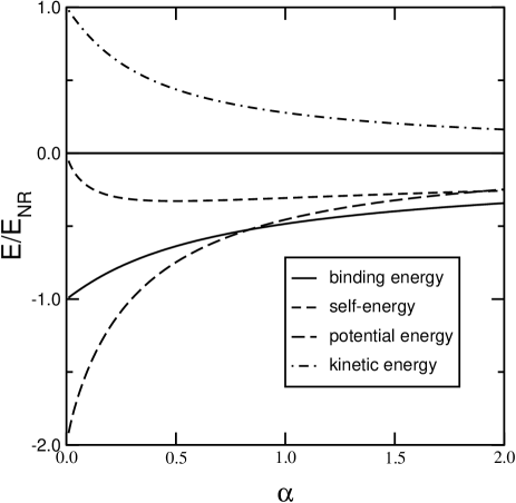
Figure 2: The properties of the ground state compared to the non-relativistic results, in the case of the masses relevant for the hydrogen atom, $m_{a}=m_{p},m_{b}=m_{e}$.

The angular integrations can be performed analytically. In order to calculate the integrals with the least numerical problems we integrate the self-energy contributions analytically, thereby avoiding the integrable singularity in the subtraction term $\Sigma(\omega_{a}+\omega_{b})$ in our numerical calculations. For the sake of completeness we give the result of a tedious but straightforward calculation:

$$\int_{0}^{\infty}\frac{k_{a}{\rm d}k_{a}}{\omega_{a}}\ln\left[\frac{\omega_{b}-E+\omega_{a}+|{k_{b}}+k_{a}|}{\omega_{b}-E+\omega_{a}+|{k_{b}}-k_{a}|}\right]_{\rm subtracted}=m_{a}^{2}\ln[m_{a}]\left(\frac{1}{{k_{b}}+\omega_{b}-E}-\frac{1}{{k_{b}}-\omega_{a}}\right)-$$ (21)

$${m_{a}^{2}}\ln[{k_{b}}+\omega_{a}]\left(\frac{\omega_{a}}{m_{a}^{2}}+\frac{\omega_{b}-E}{(E-\omega_{b}+\omega_{a})(E-\omega_{a}-\omega_{b})+m_{a}^{2}}\right)+$$

$$\frac{1}{2}\ln[\omega_{a}+\omega_{b}-E](\omega_{a}+\omega_{b}-E)\left(1+\frac{m_{a}^{2}}{(\omega_{b}-E-{k_{b}})({k_{b}}+\omega_{a})}\right)-$$

$$\frac{1}{2}\ln\left[{k_{b}}+\omega_{b}-E+\frac{m_{a}^{2}}{{k_{b}}+\omega_{a}}\right](2{k_{b}}+\omega_{a}+\omega_{b}-E)\left(1+\frac{m_{a}^{2}}{({k_{b}}+\omega_{b}-E)({k_{b}}+\omega_{a})}\right)\,.$$

The integrals converge well. With a typical compact integration coordinate the integrands are smooth bell curves in the middle of the domain, from which we know that we do not miss any contributions for small or large values of the momentum. We use a simple integration procedure and with 500 integration points we achieve a sure accuracy of 4 to 5 decimal places, which is in the same region as the systematic error due to the wave-function Ansatz. It is interesting to observe how different the self-energy contributions are for the heavy-mass and the equal-mass cases, shown in Figs. 2 and 3, respectively.

Figure 3: The properties of the ground state compared to the non-relativistic results, in the case of two equal masses, $m_{a}=m_{b}=m$.

Since Hamiltonian renormalization is not a well-established procedure, although we are convinced of its legitimacy, we repeated the same calculation with the covariant expression for the self-energy, which means that only for that part we also include the states with three particles, one anti-particle, and a photon, which leads to the known covariant result for the self-energy:

$$\Sigma_{c}=\frac{\alpha m^{2}}{2\pi}\left(1-\frac{m^{2}}{p^{2}}\right)\ln\left[\frac{m^{2}-p^{2}}{m^{2}}\right]\,,$$ (22)

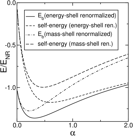
Figure 4: The comparison in the equal-mass ground-state binding energies and the self-energy contributions to that result between the case where the self-energy is renormalized on energy-shell, which includes only the forward diagram, and the case where one-particle mass-shell renormalization, from the corresponding Feynman diagram which also includes the anti-particle contributions, is used.

where $\Sigma_{c}(p^{2}=m^{2})=0$, which corresponds to the on-mass-shell renormalization; for the physical mass there is no mass correction. For small coupling the result differs only little from the restricted Fock-state result with $m_{a}=m_{b}=m$. For larger values of the coupling constant the self-energy contribution is slightly suppressed in the covariant approach, as can be seen in Fig. 4.

The heavy-mass limit yields the correct result, which reduces to the non-relativistic result in the weak-coupling limit. The latter problem is dealt with in a rather cumbersome way in the Bethe-Salpeter equation and related approaches [27], as the one-particle exchange approximation (the “ladder approximation”) does not work there.

3 Renormalization

Since we solve only the lowest non-trivial case of binding with a massless exchange field, there are many contributions we do not include. Eventually, to show that the lowest order includes most of the relevant physics of a bound state, we have to pursue the problem of convergence. This is part of the future work. However, since renormalization involves divergent contributions already present at the lowest order, also here some care is required. In the renormalization different orders in the coupling constant are mixed, while in the Hamiltonian approach some of these terms, which should be grouped together, might not appear.

For example, from the Ward identity, it would follow that one should combine wave-function renormalization of the self-energy diagrams with the vertex correction, to yield a finite answer. The former diagram appears in our equation, but the latter do not. We choose not to perform the wave-function renormalization, for one important reason: it leads to a trivial theory, with zero coupling, in our case of massless exchange particles. In the case of finite exchange-particle masses the renormalized coupling constant scales with the logarithm of the mass. Only if the vertex correction is also included, the infinite wave-function renormalization is counter-acted by the infinite charge renormalization, and only a mild dependence is left. Since these divergences are infrared divergences, it is even more physical[22] to group the wave-function renormalization with the vertex renormalization, and have both or none. In our case it is none.

If we compare our result with the work by Ji[32] we find, as expected, the opposite effect from the self-energy, because we have chosen the starting Lagrangian in such a way that we have opposite self-energy contributions; in our Lagrangian identical particles repel each other, like they should do in the Coulomb problem. However, unexpectedly, one can conclude from Ji’s work that the self-energy cures a bit of the illness of the $\phi^{3}$ theory. One would expect the binding energy to make a nose dive as the coupling constant increases, due to the unboundedness of the Hamiltonian. However, including the self-energy decreases the binding in the case of the scalar exchange as studied by Ji.

For the Bethe-Salpeter equation, with dressed propagators, it is found that the self-energy increases the binding slightly, however, these results are for a relatively large mass of the exchange particle, and the wave-function renormalization is used, which counteracts the weaker binding caused by the mass renormalization[33]. Moreover, other problems appear in the covariant Bethe-Salpeter formalism, such as unphysical solutions[33, 10], which have, at least in part, to do with the relative time-coordinate appearing in the equation. However, there are claims that these problems result from the unphysical Lagrangian[34]. For the moment we want to conclude that if renormalization is pursued beyond the simplest on-shell subtractions, many questions are still open. The same conclusion can be drawn from the work of Głazek et al.[35] on light-front Hamiltonian Yukawa theory, which seems, insofar, to confirm Ji’s findings for self-energy effects of real scalar exchange fields. However, it must be noted that in all these cases the Lagrangian was different from our Lagrangian, which in practice boiled down to the opposite sign for the self-energy. This is altogether a different problem. When we reversed the sign of the self-energy in our calculations, as a simple check, we found instabilities for $\alpha>0.5$. This is a subject for further study.

4 Conclusion

Generally, one can say that the approach advocated here is straightforward compared with the Bethe-Salpeter equation and subsequent three-dimensional reductions. The normalization is that of ordinary quantum mechanics, and spurious solutions, associated with excitations in the relative time do not occur, since the Hamiltonian framework has only one reference time. Moreover, issues concerning anti-particle content of the wave function, present in the covariant formulation, do not arise here, since the approach is based on the Fock-state truncation. Another advantage over the standard covariant approach is the absence of infrared singularities, due to the fact that the states are always off-energy-shell, and these singularities are associated with on-energy-shell states with vanishing photon momentum.

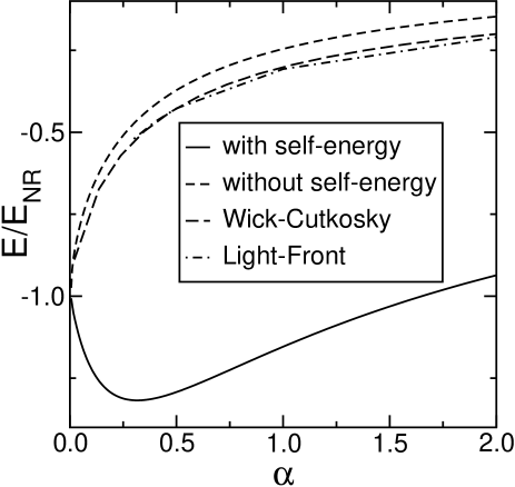
Figure 5: Comparison between the result for the full calculation, and when the self-energy terms are dropped for the equal-mass case. We also compare the results with the Wick-Cutkosky model [30, 10] and light-front results [31].

Apart from the technical advantages of this approach it is important to notice that the self-energy contributions dominate the ground state in the strong binding regime. If we perform the same calculations including all the relativistic effects except for the self-energy contribution, we find completely opposite results [31]; the binding energy is lower than the non-relativistic one, as can be seen in Fig. 5. This indicates that the usual description of strong-coupling binding in terms of exchange diagrams is, to say the least, incomplete.

5 Acknowledgments

We like to thank Prof. John Tjon, Prof. Reinhard Alkofer, and Prof. Franz Gross for remarks and discussion regarding this work. We also like to thank Jim Friar, Roland Rosenfelder, and Axel Weber for their comments.

References

- [1] W. Heitler, The quantum theory of radiation, (Clarendon, Oxford, 1954).
- [2] I.T. Todorov, Phys. Rev. D 3 (1971), 2351.
- [3] R. Blankenbecler and R. Sugar, Phys. Rev. 142 (1966) 1051.
- [4] F. Gross, Phys. Rev. 186 (1969) 1448.
- [5] H.A. Bethe and E.E. Salpeter, Phys. Rev. 82 (1951) 309. E.E. Salpeter and H.A. Bethe, ibid. 84 (1951) 1232.
- [6] F. Gross, Phys. Rev. C 26 (1982) 2203.
- [7] T. Nieuwenhuis, PhD thesis Utrecht, Oct. 1995.
- [8] D.R. Phillips and S.J. Wallace, Few Body Syst. 24 (1998) 175.
- [9] C. Itzykson and J.B. Zuber, Quantum Field Theory, (McGraw-Hill, New York, 1980).
- [10] N. Nakanishi, Prog. Phys. (Suppl.) 43 (1969) 1; ibid. 95 (1988) 1.
- [11] C. Savkli, J.A. Tjon, and F. Gross, Phys. Rev. C 60 (1999) 055210; Erratum-ibid. C 61 (2000) 069901.
- [12] Yu.A. Simonov and J.A. Tjon, Ann. Phys. (N.Y.) 228 (1993) 1.
- [13] T. Nieuwenhuis and J.A. Tjon, Phys. Rev. Lett. 77 (1996) 814.
- [14] C. Savkli, Proceedings of the European Conference on Problems in Few-Body Systems, Evora, 2000 (to be published).
- [15] O.W. Greenberg, R. Ray, and F. Schlumpf, Phys. Lett. B 353 (1995) 284.
- [16] S.J. Brodsky, H.-C. Pauli, and S.S. Pinsky, Phys. Rept. 301 (1998) 299.
- [17] S.J. Brodsky, J.R. Hiller, and G. McCartor, Phys. Rev. D 60 (1999) 054506.
- [18] P.A.M. Dirac, Rev. Mod. Phys. 21 (1949) 392.
- [19] S. Flügge, Practical quantum mechanics, (Springer, Heidelberg, 1971).
- [20] F. Bloch and A. Nordsieck, Phys. Rev. 52 (1937) 54.
- [21] S. Weinberg, The quantum theory of fields, Vol. 1, (Cambridge, Cambridge, 1995).
- [22] J.M. Jauch and F. Rohrlich, The theory of photons and electrons, (Springer, New York, 1976).
- [23] T. Murota, Prog. Phys. (Suppl.) 95 (1988) 46.
- [24] G.S. Adkins, P.M. Mitrikov, and R.N. Fell, Phys. Rev. Lett. 78 (1997) 9.
- [25] M.I. Eides, H. Grotch, and V.A. Shelyuto, hep-ph/0002158, and the references therein.
- [26] H.A. Bethe and E.E. Salpeter, Quantum mechanics of one- and two-electron atoms, (Springer, Berlin, 1957).
- [27] F. Gross, Relativistic quantum mechanics and field theory, (Wiley, New York, 1993).
- [28] J. Collins, Renormalization, (Cambridge Press, Cambridge, 1984).
- [29] G. Baym, Phys. Rev. 117 (1959) 886.
- [30] G.C. Wick, Phys. Rev. 96 (1954) 1124; R.E. Cutkosky, ibid. 1135.
- [31] M. Mangin-Brinet and J. Carbonell, Phys. Lett. B 474 (2000) 237.
- [32] C.R. Ji, Phys. Lett B 322 (1994) 389.
- [33] S. Ahlig and R. Alkofer, Ann. Phys. (N.Y.) 275 (1999) 113.
- [34] R. Rosenfelder and A.W. Schreiber, Phys. Rev. D 53 (1996) 3337 & 3354.
- [35] S. Głazek et al, Phys. Rev. D 47 (1993) 1599.