The Probability Density of the Mass of the Standard Model Higgs Boson

Abstract

The LEP Collaborations have reported a small excess of events in their combined Higgs boson analysis at center of mass energies $\sqrt{s}\buildrel<\over{{}_{\sim}}208$ GeV. In this communication, I present the result of a calculation of the probability distribution function of the Higgs boson mass which can be rigorously obtained if the validity of the Standard Model is assumed. It arises from the combination of the most recent set of precision electroweak data and the current results of the Higgs searches at LEP 2.

Combining all Higgs decay channels and experiments, the LEP Collaborations report a $2.5\sigma$ excess in their data [1]. The probability that this is due to an upward fluctuation of the background is 0.6%. Of course, the Higgs boson has been searched for in many different energy bins, and there is an infinitely large energy range out of reach, so that one expects to observe an upward fluctuation somewhere. It is therefore difficult to interpret these numbers, and it would be imprudent to conclude that the Higgs boson has been found with 99.4% probability.

In this communication, I present the answer to a different but related question, which is Given the data, what is the probability that the Higgs boson is within reach of LEP 2? This question can be answered unambiguously once the probability distribution of the Higgs boson mass, $M_{H}$, has been constructed. This is not possible given the Higgs search results at LEP 2 by themselves, regardless of how strong a signal is observed there. The reason is that there is an infinite domain of a priori possible values of $M_{H}$ beyond the kinematic reach of LEP 2. As a result, the $M_{H}$ distribution is improper, i.e., it is asymptotically non-zero. Including the electroweak precision data, however, renders it sufficiently convergent and a proper integration is possible.

The electroweak precision data by itself, especially $Z$ pole asymmetries and the $W$ boson mass, is now precise enough to constrain $M_{H}$ significantly, as can be seen from Fig. 1.

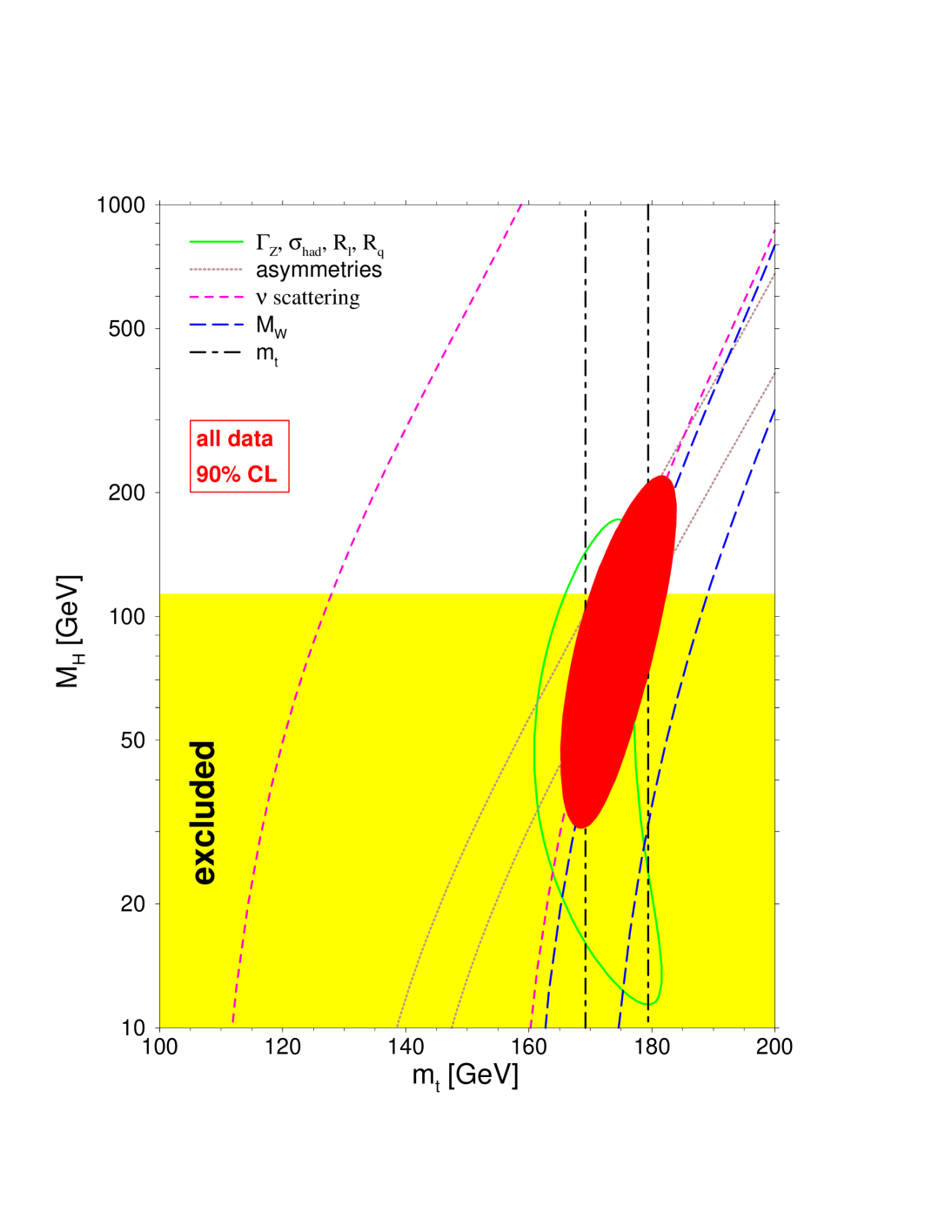
FIG. 1.: Constraints on $M_{H}$ from various sets of precision data as a function of the top quark mass. For the individual data sets I show $1\sigma$ contours, while the ellipse for all data refers to the 90% CL. The excluded region by LEP 2, $M_{H}<113.2$ GeV (95% CL), is also indicated.

Including the latest updates as presented at the 2000 summer conferences, I find from a global fit to all data using the package GAPP [2],

$$M_{H}=86^{+48}_{-32}\mbox{ GeV}.$$ (1)

Note, that by definition the central value in Eq. (1) maximizes the likelihood, $Ne^{-\chi^{2}(M_{H})/2}$, and that correlations with other parameters, $\xi^{i}$, are accounted for, since minimization w.r.t. these is understood, $\chi^{2}\equiv\chi^{2}_{\rm min}$. The error is the standard $1\sigma$ uncertainty ($\Delta\chi^{2}=1$). The 68.27% central confidence interval,

$$53\mbox{ GeV}\leq M_{H}\leq 131\mbox{ GeV},$$ (2)

differs slightly from Eq. (1) due to the non-Gaussian (asymmetric) distribution of $\ln M_{H}$. The 90% central confidence interval yields,

$$38\mbox{ GeV}\leq M_{H}\leq 173\mbox{ GeV}.$$ (3)

The right hand side of Eq. (3), i.e., the 95% upper limit, does not take into account the direct search results of the LEP Collaborations. Negative search results will increase the upper limit, because the probability distribution function is effectively being renormalized. For example, in a previous analysis [3] we found that the Higgs exclusion curve presented by the LEP Collaborations increased the 95% upper limit by 30 GeV.

The use of the Higgs exclusion curve, however, is only appropriate if no indication of an excess is observed. In general, it is more appropriate to consider the likelihood ratio for the data,

$$Q_{\rm LEP~{}2}=\frac{{\cal L}({\rm data|signal+background})}{{\cal L}({\rm data|background})},$$ (4)

where both the numerator and the denominator are functions of $M_{H}$. The quantity,

$$\Delta\chi^{2}({\rm direct})\equiv-2\ln Q_{\rm LEP~{}2}$$ (5)

can then be added to the $\chi^{2}$-function obtained from the precision data. If the signal hypothesis gives a better (worse) description of the data than the background only hypothesis we find a negative (positive) contribution to the total $\chi^{2}$. Note, that this is a consistent treatment also in the case of a large downward fluctuation of the background or even if no events are observed at all. Use of $Q_{\rm LEP~{}2}$ had been originally advocated in Ref. [5] (see Eq. (23) in that reference).

This treatment can be rigorously justified within the framework of Bayesian statistics [6, 7], which is particularly suited for parameter estimation. Bayesian methods are based on Bayes theorem [6],

$$p(M_{H}|{\rm data})=\frac{p({\rm data}|M_{H})p(M_{H})}{p({\rm data})},$$ (6)

which must be satisfied once the likelihood, $p({\rm data}|M_{H})$, and prior distribution, $p(M_{H})$, are specified. $p(data)\equiv\int p({\rm data}|M_{H})p(M_{H})dM_{H}$ in the denominator provides the proper normalization of the posterior distribution on the left hand side. Depending on the case at hand, the prior can

1. contain additional information not included in the likelihood model,

2. contain likelihood functions obtained from previous measurements,

3. or be chosen non-informative.

Of course, the posterior does not depend on how information is separated into the likelihood and the prior. As for the present case, I choose the informative prior,

$$p(M_{H})=Q_{\rm LEP~{}2}~{}p^{\rm non-inf}(M_{H}),$$ (7)

where the non-informative part of the prior will be chosen as

$$p^{\rm non-inf}(M_{H})=M_{H}^{-1}.$$ (8)

This choice corresponds to a flat prior in the variable $\ln M_{H}$, and there are various ways to justify it [7]. One rationale is that a flat distribution is most natural for a variable defined over all the real numbers. This is the case for $\ln M_{H}$ but not $M_{H}^{2}$. Also, it seems that a priori it is equally likely that $M_{H}$ lies, say, between 30 and 40 GeV, or between 300 and 400 GeV. In any case, the sensitivity of the posterior to the (non-informative) prior diminishes rapidly with the inclusion of more data. As discussed before, $p(M_{H})$ is an improper prior but the likelihood constructed from the precision measurements will provide a proper posterior.

Occasionally, the Bayesian method is criticized for the need of a prior, which would introduce unnecessary subjectivity into the analysis. Indeed, care and good judgement is needed, but the same is true for the likelihood model, which has to be specified in any statistical model. Moreover, it is appreciated among Bayesian practitioners, that the explicit presence of the prior can be advantageous: it manifests model assumptions and allows for sensitivity checks. From the theorem (6) it is also clear that any other method must correspond, mathematically, to specific choices for the prior. Thus, Bayesian methods are more general and differ rather in attitude: by their strong emphasis on the entire posterior distribution and by their first principles setup.

Including $Q_{\rm LEP~{}2}$ in this way, one obtains the 95% CL upper limit $M_{H}\leq 201$ GeV, i.e. notwithstanding the observed excess events, the information provided by the Higgs searches at LEP 2 increase the upper limit by 28 GeV.

Given extra parameters, $\xi^{i}$, the distribution function of $M_{H}$ is defined as the marginal distribution, $p(M_{H}|{\rm data})=\int p(M_{H},\xi^{i}|{\rm data})\prod_{i}p(\xi^{i})d\xi^{i}$. If the likelihood factorizes, $p(M_{H},\xi^{i})=p(M_{H})p(\xi^{i})$, the $\xi^{i}$ dependence can be ignored. If not, but $p(\xi^{i}|M_{H})$ is (approximately) multivariate normal, then

$$\chi^{2}(M_{H},\xi^{i})=\chi^{2}_{\rm min}(M_{H})+$$

$${1\over 2}\frac{\partial^{2}\chi^{2}(M_{H})}{\partial\xi_{i}\partial\xi_{j}}(\xi^{i}-\xi^{i}_{\rm min}(M_{H}))(\xi^{j}-\xi^{j}_{\rm min}(M_{H})).$$

The latter applies to our case, where $\xi^{i}=(m_{t},\alpha_{s},\alpha(M_{Z}))$. Integration yields,

$$p(M_{H}|{\rm data})\sim\sqrt{\det E}\,e^{-\chi^{2}_{\rm min}(M_{H})/2},$$ (9)

where the $\xi^{i}$ error matrix, $E=(\frac{\partial^{2}\chi^{2}(M_{H})}{\partial\xi_{i}\partial\xi_{j}})^{-1}$, introduces a correction factor with a mild $M_{H}$ dependence. It corresponds to a shift relative to the standard likelihood model, $\chi^{2}(M_{H})=\chi^{2}_{\rm min}(M_{H})+\Delta\chi^{2}(M_{H})$, where

$$\Delta\chi^{2}(M_{H})\equiv\ln\frac{\det E(M_{H})}{\det E(M_{Z})}.$$ (10)

This effect tightens the $M_{H}$ upper limit by 1 GeV.

I also include theory uncertainties from uncalculated higher orders. This increases the upper limit by 5 GeV,

$$M_{H}\leq 205\mbox{ GeV}\mbox{ (95\% CL)}.$$ (11)

The entire probability distribution is shown in Fig. 2. Taking the data at face value, there is (as expected) a significant peak around $M_{H}=115$ GeV, but more than half of the probability is for Higgs boson masses above the kinematic reach of LEP 2 (the median is at $M_{H}=119$ GeV). However, if one would double the integrated luminosity and assume that the results would be similar to the present ones, one would find most of the probability concentrated around the peak. A similar statement will apply to Run II of the Tevatron at a time when about 3 to 5 ${\rm fb}^{-1}$ of data have been collected.

FIG. 2.: Probability distribution function for the Higgs boson mass. The probability is shown for bin sizes of 1 GeV. Included are all available direct and indirect data. The shaded and unshaded regions each mark 50% probability.

The described method is robust within the SM, but it should be cautioned that $M_{H}$ extracted from the precision data is strongly correlated with certain new physics parameters. Likewise, the Higgs searches at LEP 2 depend on the predictions of signal and background expectations which are strictly calculable only within a specified theory. This note focussed on the Standard Model Higgs boson.

Acknowledgements:

This work was supported in part by the US Department of Energy grant EY–76–02–3071.

REFERENCES

- [1] T. Junk, Combined LEP Higgs Searches, Talk presented at the LEP Fest 2000, CERN, October 2000.
-
[2]
http://www.physics.upenn.edu/erler/electroweak;
J. Erler, Global Fits to Electroweak Data Using GAPP, e-print hep-ph/0005084, to appear in Physics at RUN II: QCD and Weak Boson Physics. - [3] J. Erler and P. Langacker, Electroweak Model and Constraints on New Physics, p. 95 in Ref. [4].
- [4] D.E. Groom et al., Eur. Phys. J. C15, 1 (2000).
- [5] G. d’Agostini and G. Degrassi, Eur. Phys. J. C10, 663 (1999).
- [6] T. Bayes, Phil. Trans. 53, 370 (1763), reprinted in Biometrica 45, 296 (1958).
- [7] For a comprehensive introduction and review of applied statistics and data analysis see A. Gelman, J.B. Carlin, H.S. Stern, and D.B. Rubin, Bayesian Data Analysis, (Chapman & Hall, London, 1995).