Lepton Flavor Violation in the Two Higgs Doublet Model type III

Abstract

We consider the Two Higgs Doublet Model (2HDM) of type III which leads to Flavour Changing Neutral Currents (FCNC) at tree level in the leptonic sector. In the framework of this model we can have, in principle, two situations: the case (a) when both doublets acquire a vacuum expectation value different from zero and the case (b) when only one of them is not zero. In addition, we show that we can make two types of rotations for the flavor mixing matrices which generates four types of lagrangians, with the rotation of type I we recover the case (b) from the case (a) in the limit $\tan\beta\rightarrow\infty$, and with the rotation of type II we obtain the case (b) from (a) in the limit $\tan\beta\rightarrow 0.\;$Moreover, two of the four possible lagrangians correspond to the models of types I and II plus Flavor Changing (FC) interactions. The analitical expressions of the partial lepton number violating widths $\Gamma\left(\mu\rightarrow eee\right)$ and $\Gamma(\mu\rightarrow e\gamma)\;$are derived for the cases (a) and (b) and both types of rotations. In all cases these widths go asymptotically to zero in the decoupling limit for all Higgses. We present from our analysis upper bounds for the flavour changing transition $\mu\rightarrow e,$ and we show that such bounds are sensitive to the VEV structure and the type of rotation utilized.

I Introduction

Flavor Changing Neutral Currents (FCNC) are forbidden at tree level in the Standard Model (SM). However, they could be present at one loop level as in the case of $b\rightarrow s\gamma$ bsg , $K^{0}\rightarrow\mu^{+}\mu^{-}$ kmm , $K^{0}-\overline{K}^{0}$ koko , $t\rightarrow c\gamma$ tcg etc. In general, many extensions of the SM permit, however FCNC at tree level. The introduction of new representations of fermions different from doublets produce them by means of the Z-coupling 2 . In addition, they are generated at tree level in the Yukawa sector by adding a second doublet to the SM wolf . Such couplings also appear in SUSY theories without R-parity R1 . Theories with FCNC were previously considered unatractive because they were strongly constrained experimentally, especially due to the small $K_{L}-K_{S}\;$mass difference. Nevertheless, nowadays it is hoped to observe such physical processes in laboratory, as a result many theories were proposed (see above).

Owing to the continuous improvements in experimental accuracies, Lepton Flavor Violation (LFV) has become a very important possible source of new physics. Experiments to search directly for LFV have been performed for many years, all with null results so far. Experimental limits have resulted from searches for $K_{L}^{0}\to\mu^{+}e^{-}$ arisaka , $K_{L}^{0}\to\pi^{0}\mu^{+}e^{-}$ plb , $K^{+}\to\pi^{+}\mu^{+}e^{-}$ lee , $\mu^{+}\to e^{+}\gamma$ bolton , $\mu^{+}\to e^{+}e^{+}e^{-}$ bell and $\mu^{-}N\to e^{-}N$ doh .

There are several mechanisms to avoid FCNC at tree level. Glashow and Weinberg gw proposed a discrete symmetry in the Two Higgs Doublet Model (2HDM) which forbids the couplings that generate such rare decays, hence they do not appear at tree level. Another possibility is to consider heavy exchange of scalar or pseudoscalar Higgs fields Sher91 or by cancellation of large contributions with opposite sign. Another mechanism was proposed by Cheng and Sher arguing that a natural value for the FC couplings from different families should be of the order of the geometric average of their Yukawa couplings ChengSher .

Taking this natural assumption and since Yukawa couplings in the SM vary with mass, it is plausible that the same occurs for FC couplings. Hence it is expected that FCNC involving the third generation can be larger, while the ones involving the first generation are hoped to be small Sher91 , Reina . Another clue that suggests large mixing between the second and third generation in the charged leptonic sector, is the large mixing between second and third generation of the neutral leptonic sector. This is predicted by experiments with atmospheric neutrinos Fukuda .

The increasing interest in LFV processes is due to the strong restrictions that experiments have imposed on them. This consequently determines small regions of parameters for new physics of any theory beyond the SM. Some specific decays have been widely studied within the framework of supersymmetric extensions, because in Supersymmetric theories the presence of FCNC induced by R-parity violation generates massive neutrinos and neutrino oscillations Kaustubh . In recent papers the decays $\mu\rightarrow e\gamma\;$and $\mu\rightarrow 3e\;$with polarized muons have been examined in the context of supersymmetric grand unified theories to get bounds in the $m_{\widetilde{e}_{R}}-\left|A_{0}\right|\;$plane Okada .

On the other hand, a muon collider could provide very interesting new constraints on FCNC, for example $\mu\mu\rightarrow\mu\tau(e\tau)\;$ mediated by Higgs exchange SherCollider which test the mixing between the second and third generations. Additionally, the muon collider could be a Higgs factory and it is well known that the Higgs sector is crucial for FCNC Workshop . Finally, effects on the coupling of muon and tau in the 2HDM framework owing to anomalous magnetic moment of the muon could be significantly improved by E821 experiment at Brookhaven National Laboratory SherCollider .

Additionally, in the quark sector bounds on LFV come from $\Delta F=2$ processes, rare B-decays, $Z\to\overline{b}b$ and the $\rho$-parameter ARS . Reference ARS also explored the implications of FCNC at tree level for $e^{+}e^{-}(\mu^{+}\mu^{-})\to t\overline{c}+\overline{t}c$, $t\to c\gamma(Z,g)$, $D^{0}-\overline{D}^{0}$ and $B^{0}_{s}-\overline{B}^{0}_{s}$. Moreover, there are other important processes involving FCNC. For instance, the decay $B^{-}(D^{-})\rightarrow K^{-}\mu^{+}\tau^{-}\;$ which depends on $\mu-\tau\;$mixing and vanishes in the SM. Hence it is very sensitive to new physics. Another one is $B^{-}(D^{-})\rightarrow K^{-}\mu^{+}e^{-}\;$whose form factors have been calculated in Sher91 , nosotros .

The simplest model which exhibits FCNC at tree level is the model with one extra Higgs doublet, known as the two Higgs doublet model (2HDM). There are several kinds of such models. In the model type I, one Higgs Doublet provides masses to the up and down quarks, simultaneously. In the model type II, one Higgs doublet gives masses to the up quarks and the other one to the down quarks. These former two models have the discrete symmetry mentioned above to avoid FCNC at tree level gw . However, the discrete symmetry is not necessary in whose case both doublets generate the masses of the quarks of up-type and down-type, simultaneously. In the literature, the latter is known as the model type III III . It has been used to look for physics beyond the SM and specifically for FCNC at tree level ARS , Sher91 . In general, both doublets could acquire a vacuum expectation value (VEV), but we can absorb one of them redefining the Higgs fields properly. Nevertheless, we shall show that a substantial difference arises from the case in which both doublets get the VEV, and therefore we will study the model type III considering two cases. In the first case, the two Higgs doublets acquire VEV (case (a)). In the second one, only one Higgs doublet acquire VEV (case (b)). In the latter case the free parameter $\tan\beta$ is removed from the theory making the analysis simpler.

In section II, we describe the model and define the notation we shall use throughout the document. In section III, we show that we can make two kinds of rotations for the flavor mixing matrices which generates four types of lagrangians, and that in the framework of the first rotation we arrive to the case (b) from the case (a) in the limit $\tan\beta\rightarrow\infty$, while with the second rotation we obtain (b) from (a) in the limit $\tan\beta\rightarrow 0.\;$Furthermore, we find that two of the four possible lagrangians correspond to the models of types I and II plus Flavor Changing (FC) interactions.

In section IV we get bounds on LFV in the 2HDM type III based on the decays $\mu\rightarrow e\gamma$ and $\mu\rightarrow eee$. Such decays are examined in the framework of both cases (a) and (b) according to the classification made above, and with both types of rotations. We find that such constraints depend on whether we use cases (a) or (b) and on what kind of rotation is utilized.

II The Model

The 2HDM type III is an extension of the SM plus a new Higgs doublet and three new Yukawa couplings in the quark and leptonic sectors. The mass terms for the up-type or down-type sectors depends on two matrices or two Yukawa couplings. The rotation of the quarks and leptons allows us to diagonalize one of the matrices but not both simultaneously, so one of the Yukawa couplings remains non-diagonal, generating the FCNC at tree level.

The Yukawa’s Lagrangian is as follow

$$-\pounds_{Y} = \eta_{ij}^{U,0}\overline{Q}_{iL}^{0}\widetilde{\Phi}_{1}U_{jR}^{0}+\eta_{ij}^{D,0}\overline{Q}_{iL}^{0}\Phi_{1}D_{jR}^{0}+\eta_{ij}^{E,0}\overline{l}_{iL}^{0}\Phi_{1}E_{jR}^{0}$$

$$+ \xi_{ij}^{U,0}\overline{Q}_{iL}^{0}\widetilde{\Phi}_{2}U_{jR}^{0}+\xi_{ij}^{D,0}\overline{Q}_{iL}^{0}\Phi_{2}D_{jR}^{0}+\xi_{ij}^{E,0}\overline{l}_{iL}^{0}\Phi_{2}E_{jR}^{0}+h.c.$$

where $\Phi_{1,2}\;$are the Higgs doublets,$\;\eta_{ij}^{0}\;$and $\xi_{ij}^{0}\;$ are non-diagonal $3\times 3\;$non-dimensional matrices and $i$, $j$ are family indices. $D\;$refers to the three down quarks $D\equiv\left(d,s,b\right)^{T},\;U\;$refers to the three up quarks $U\equiv\left(u,c,t\right)^{T}\;$and $E\;$to the three charged leptons. The superscript $0$ indicates that the fields are not mass eigenstates yet. In the so-called model type I, the discrete symmetry forbids the terms proportional to $\xi_{ij}^{0},\;$meanwhile in the model type II the same symmetry forbids terms proportional to $\xi_{ij}^{U,0},\;\eta_{ij}^{D,0},\eta_{ij}^{E,0}.$

In this kind of model (type III), we consider two cases. In the case (a) we assume the VEV as

$$\left\langle\Phi_{1}\right\rangle_{0}=\left(\begin{array}[]{c}0\\ v_{1}/\sqrt{2}\end{array}\right)\;\;,\;\;\left\langle\Phi_{2}\right\rangle_{0}=\left(\begin{array}[]{c}0\\ v_{2}/\sqrt{2}\end{array}\right)$$

and we take the complex phase of $v_{2}\;$equal to zero since we are not interested in CP violation. The mass eigenstates of the scalar fields are given by moda

$$\left(\begin{array}[]{c}G_{W}^{\pm}\\ H^{\pm}\end{array}\right) = \left(\begin{array}[]{cc}\cos\beta&\sin\beta\\ -\sin\beta&\cos\beta\end{array}\right)\left(\begin{array}[]{c}\phi_{1}^{\pm}\\ \phi_{2}^{\pm}\end{array}\right),$$ (8)

$$\left(\begin{array}[]{c}G_{Z}^{0}\\ A^{0}\end{array}\right) = \left(\begin{array}[]{cc}\cos\beta&\sin\beta\\ -\sin\beta&\cos\beta\end{array}\right)\left(\begin{array}[]{c}\sqrt{2}Im\phi_{1}^{0}\\ \sqrt{2}Im\phi_{2}^{0}\end{array}\right),$$ (15)

$$\left(\begin{array}[]{c}H^{0}\\ h^{0}\end{array}\right) = \left(\begin{array}[]{cc}\cos\alpha&\sin\alpha\\ -\sin\alpha&\cos\alpha\end{array}\right)\left(\begin{array}[]{c}\sqrt{2}Re\phi_{1}^{0}-v_{1}\\ \sqrt{2}Re\phi_{2}^{0}-v_{2}\end{array}\right)$$ (22)

where $\tan\beta=v_{2}/v_{1}\;$and $\alpha\;$is the mixing angle of the CP-even neutral Higgs sector. $G_{Z(W)}\;$are the would-be Goldstone bosons for $Z\left(W\right)$, respectively. And $A^{0}\;$is the CP-odd neutral Higgs. $H^{\pm}\;$are the charged physical Higgses.

The case (b) corresponds to the case in which the VEV are taken as

$$\left\langle\Phi_{1}\right\rangle_{0}=\left(\begin{array}[]{c}0\\ v_{1}/\sqrt{2}\end{array}\right)\;\;,\;\;\ \left\langle\Phi_{2}\right\rangle_{0}=\left(\begin{array}[]{c}0\\ 0\end{array}\right).$$ (23)

The mass eigenstates scalar fields in this case are modb

$$G_{W}^{\pm} = \phi_{1}^{\pm}\;\;\;\;\;\;,\;\;\;\;\;\;H^{\pm}=\phi_{2}^{\pm}\;\;,$$

$$G_{Z}^{0} = \sqrt{2}Im\phi_{1}^{0}\;\;\;\;,\;\;\;\;A^{0}=\sqrt{2}Im\phi_{2}^{0},$$ (24)

and the neutral CP-even fields are the same as in the former model just replacing $v_{2}=0.\;$A very important difference between both models is that $G_{Z\left(W\right)}\;$is a linear combination of components of $\Phi_{1}\;$and $\Phi_{2}$ in the model (a), meanwhile in the model (b) is a component of the doublet $\Phi_{1}.$

III Generation of models type I and II from type III

To convert the lagrangian (II) into mass eigenstates we make the unitary transformations

$$D_{L,R} = \left(V_{L,R}\right)D_{L,R}^{0}\;$$ (25)

$$U_{L,R} = \left(T_{L,R}\right)U_{L,R}^{0}\;$$ (26)

 

from which we obtain the mass matrices. In the framework of case (a)

$$M_{D}^{diag} = V_{L}\left[\frac{v_{1}}{\sqrt{2}}\eta^{D,0}+\frac{v_{2}}{\sqrt{2}}\xi^{D,0}\right]V_{R}^{\dagger}$$ (27)

$$M_{U}^{diag} = T_{L}\left[\frac{v_{1}}{\sqrt{2}}\eta^{U,0}+\frac{v_{2}}{\sqrt{2}}\xi^{U,0}\right]T_{R}^{\dagger}$$ (28)

From (27), (28) we can solve for $\xi^{D,0},\xi^{U,0}\;$obtaining

$$\xi^{D,0} = \frac{\sqrt{2}}{v_{2}}V_{L}^{\dagger}M_{D}^{diag}V_{R}-\frac{v_{1}}{v_{2}}\eta^{D,0}$$ (29)

$$\xi^{U,0} = \frac{\sqrt{2}}{v_{2}}T_{L}^{\dagger}M_{D}^{diag}T_{R}-\frac{v_{1}}{v_{2}}\eta^{U,0}$$ (30)

Let us call the eqs (29), (30), rotations of type I, replacing them into (II) the expanded Lagrangian for up and down sectors are

$$-\pounds_{Y\left(u\right)}^{\left(a,I\right)} = -\frac{g\cot\beta}{M_{W}}\overline{U}M_{U}^{diag}KP_{L}DH^{+}-\frac{g}{M_{W}}\overline{U}M_{U}^{diag}KP_{L}DG^{+}$$ (31)

$$+\frac{g}{\sqrt{2}M_{W}\sin\beta}\overline{U}M_{U}^{diag}U\left(\sin\alpha H^{0}+\cos\alpha h^{0}\right)$$

$$-\frac{ig}{\sqrt{2}M_{W}}\overline{U}M_{U}^{diag}\gamma_{5}UG^{0}-\frac{ig\cot\beta}{\sqrt{2}M_{W}}\overline{U}M_{U}^{diag}\gamma_{5}UA^{0}$$

$$+\frac{1}{\sin\beta}\overline{U}\eta^{U}KP_{L}DH^{+}-\frac{1}{\sqrt{2}\sin\beta}\overline{U}\eta^{U}U\left[\sin\left(\alpha-\beta\right)H^{0}+\cos\left(\alpha-\beta\right)h^{0}\right]$$

$$+\frac{i}{\sqrt{2}\sin\beta}\overline{U}\eta^{U}\gamma_{5}UA^{0}+h.c.+\text{leptonic\ sector}.$$

$$-\pounds_{Y\left(d\right)}^{\left(a,I\right)} = \frac{g\cot\beta}{M_{W}}\overline{U}KM_{D}^{diag}P_{R}DH^{+}+\frac{g}{M_{W}}\overline{U}KM_{D}^{diag}P_{R}DG^{+}$$ (32)

$$+\frac{g}{\sqrt{2}M_{W}\sin\beta}\overline{D}M_{D}^{diag}D\left(\sin\alpha H^{0}+\cos\alpha h^{0}\right)$$

$$+\frac{ig}{\sqrt{2}M_{W}}\overline{D}M_{D}^{diag}\gamma_{5}DG^{0}+\frac{ig\cot\beta}{\sqrt{2}M_{W}}\overline{D}M_{D}^{diag}\gamma_{5}DA^{0}$$

$$-\frac{1}{\sin\beta}\overline{U}K\eta^{D}P_{R}DH^{+}-\frac{1}{\sqrt{2}\sin\beta}\overline{D}\eta^{D}D\left[\sin\left(\alpha-\beta\right)H^{0}+\cos\left(\alpha-\beta\right)h^{0}\right]$$

$$-\frac{i}{\sqrt{2}\sin\beta}\overline{D}\eta^{D}\gamma_{5}DA^{0}+h.c.+\text{leptonic\ sector.}$$

where $K\;$is the CKM matrix. The superindex $(a,I)\;$refers to the case (a) and rotation type I.

It is easy to check that if we add (31) and (32) we obtain a lagrangian consisting of the one in the 2HDM type I moda , plus the FC interactions. Therefore, we obtain the lagrangian of type I from eqs (31) and (32) by setting $\eta^{D}=\eta^{U}$ $=0.\;$In addition, it is observed that the case (b) in both up and down sectors can be calculated just taking the limit $\tan\beta\rightarrow\infty$.

On the other hand, from (27), (28) we can also solve for $\eta^{D,0},\eta^{U,0}\;$instead of, to get

$$\eta^{D,0} = \frac{\sqrt{2}}{v_{1}}V_{L}^{\dagger}M_{D}^{diag}V_{R}-\frac{v_{2}}{v_{1}}\xi^{D,0}$$ (33)

$$\eta^{U,0} = \frac{\sqrt{2}}{v_{1}}T_{L}^{\dagger}M_{U}^{diag}T_{R}-\frac{v_{2}}{v_{1}}\xi^{U,0}$$ (34)

which we call rotations of type II, replacing them into (II) the expanded lagrangian for up and down sectors become

$$-\pounds_{Y\left(u\right)}^{\left(a,II\right)} = \frac{g}{M_{W}}\tan\beta\overline{U}M_{U}^{diag}KP_{L}DH^{+}-\frac{g}{M_{W}}\overline{U}M_{U}^{diag}KP_{L}DG^{+}$$ (35)

$$+\frac{g}{\sqrt{2}M_{W}\cos\beta}\overline{U}M_{U}^{diag}U\left(\cos\alpha H^{0}-\sin\alpha h^{0}\right)-\frac{ig}{\sqrt{2}M_{W}}\overline{U}M_{U}^{diag}\gamma_{5}UG^{0}$$

$$+\frac{ig\tan\beta}{\sqrt{2}M_{W}}\overline{U}M_{U}^{diag}\gamma_{5}UA^{0}-\frac{1}{\cos\beta}\overline{U}\xi^{U}KP_{L}DH^{+}$$

$$+\frac{1}{\sqrt{2}\cos\beta}\overline{U}\xi^{U}U\left[\sin\left(\alpha-\beta\right)H^{0}+\cos\left(\alpha-\beta\right)h^{0}\right]-\frac{i}{\sqrt{2}\cos\beta}\overline{U}\xi^{U}\gamma_{5}UA^{0}$$

$$+h.c.+\text{leptonic sector}$$

$$-\pounds_{Y(d)}^{(a,II)} = -\frac{g\tan\beta}{M_{W}}\overline{U}KM_{D}^{diag}P_{R}DH^{+}+\frac{g}{M_{W}}\overline{U}KM_{D}^{diag}P_{R}DG^{+}$$ (36)

$$+\frac{g}{\sqrt{2}M_{W}\cos\beta}\overline{D}M_{D}^{diag}D\left(\cos\alpha H^{0}-\sin\alpha h^{0}\right)+\frac{ig}{\sqrt{2}M_{W}}\overline{D}M_{D}^{diag}\gamma_{5}DG^{0}$$

$$-\frac{ig\tan\beta}{\sqrt{2}M_{W}}\overline{D}M_{D}^{diag}\gamma_{5}DA^{0}+\frac{1}{\cos\beta}\overline{U}K\xi^{D}P_{R}DH^{+}$$

$$+\frac{1}{\sqrt{2}\cos\beta}\overline{D}\xi^{D}D\left[\sin\left(\alpha-\beta\right)H^{0}+\cos\left(\alpha-\beta\right)h^{0}\right]+\frac{i}{\sqrt{2}\cos\beta}\overline{D}\xi^{D}\gamma_{5}DA^{0}$$

$$+h.c.+\;\text{leptonic sector}$$

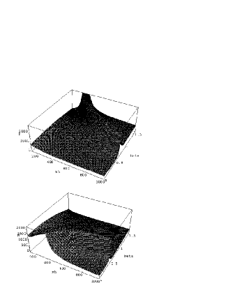
Figure 1: The figure 1 corresponds to 3D plots of the fraction of FC couplings coming from the ratio of the muon contribution and tau contribution in the radiative corrections for the process $\mu\to e\gamma$. With $\alpha=\pi/16$, $m_{H^{0}}=300$ GeV and $m_{A^{0}}$ is decoupled. The figure on the top corresponds to (aI) and the other one to (aII).

In this situation the case (b) is obtained in the limit $\tan\beta\rightarrow 0,\;$for up and down sectors. Moreover, if we add the lagrangians (31) and (36) we find the lagrangian of the 2HDM type II moda plus the FC interactions. Similarly like before, lagrangian type II is obtained setting $\xi^{D}=\eta^{U}=0.$ Therefore, lagrangian type II is generated by making a rotation of type I in the up sector and a rotation of type II in the down sector, it is valid since $\xi^{U}\;$and $\xi^{D}\;$are independent each other and same to $\eta^{U,D}.\;$In addition, we can build two additional lagrangians by adding $\pounds_{Y(u)}^{(a,II)}+\pounds_{Y(d)}^{(a,II)}\;$and $\pounds_{Y(u)}^{(a,II)}+\pounds_{Y(d)}^{(a,I)}$. So four models are generated from the case (a). On the other hand, interactions involving Goldstone bosons are the same in all the models in the R-gauge, while in the unitary gauge they vanish moda .

Finally, we can realize that in both models (a) and (b) with both types of rotations FCNC processes vanishes when all Higgses are decoupled, we shall prove it by using the rare processes $\mu\rightarrow eee\;$and $\mu\rightarrow e\gamma$.

IV LFV processes

In the present work, we study the processes $\;\mu\rightarrow e\gamma$ and $\mu\rightarrow eee\;$ in the 2HDM type III. The decay width of $\mu\rightarrow e\gamma\;$in both models (a) and (b) comes from one loop corrections, where we have used a muon running in the loop. The first interaction vertex is proportional to the muon mass and the final vertex is proportional to the flavor changing transition $\mu\rightarrow e.$ The decay widths in the two types of rotations are given by

$$\Gamma^{(a,I)}\left(\mu\rightarrow e\gamma\right) = \frac{4G_{F}\alpha m_{\mu}^{7}\eta_{\mu e}^{2}}{\sqrt{2}\sin^{4}\beta}\left|\sin\alpha\sin\left(\alpha-\beta\right)F_{1}(m_{H^{0}})+\cos\alpha\cos\left(\alpha-\beta\right)F_{1}(m_{h^{0}})-\cos\beta F_{2}(m_{A^{0}})\right|^{2}$$

$$\Gamma^{\left(a,II\right)}\left(\mu\rightarrow e\gamma\right) = \frac{4G_{F}\alpha m_{\mu}^{7}\xi_{\mu e}^{2}}{\sqrt{2}\cos^{4}\beta}\left|-\cos\alpha\sin\left(\alpha-\beta\right)F_{1}(m_{H^{0}})+\sin\alpha\cos\left(\alpha-\beta\right)F_{1}(m_{h^{0}})-\tan\beta F_{2}(m_{A^{0}})\right|^{2}$$ (37)

where

$$F_{1}(x) = \frac{\log[x^{2}/m_{\mu}^{2}]}{4\pi^{2}x^{2}}$$

$$F_{2}(x) = \frac{-\log\left[x^{2}/m_{\mu}^{2}\right]}{8\pi^{2}x^{2}}$$ (38)

Figure 2: The figure 2 illustrate the differences between the models (aI) and (aII) respect to the parameter $\tan\beta$. We have decoupled the higgses masses $m_{H^{0}}=300$ GeV and $m_{A^{0}}$ and taken $\alpha=\pi/16$ and $m_{h^{0}=}300$ GeV. The curve that increases with $\beta$ corresponds to the model (aI).

The decay widths for the process $\mu\rightarrow eee\;$ in the two cases read

$$\Gamma^{\left(a,I\right)}\left(\mu\rightarrow eee\right) = \frac{2G_{F}m_{\mu}^{5}m_{e}^{2}N_{\mu e}^{2}}{\sqrt{2}1024\pi^{3}\sin^{4}\beta}\left|\frac{\sin\alpha\sin\left(\alpha-\beta\right)}{m_{H^{0}}^{2}}\right.$$

$$+ \left.\frac{\cos\alpha\cos\left(\alpha-\beta\right)}{m_{h^{0}}^{2}}-\frac{\cos\beta}{m_{A^{0}}^{2}}\right|^{2},$$

$$\Gamma^{\left(a,II\right)}\left(\mu\rightarrow eee\right) = \frac{2G_{F}m_{\mu}^{5}m_{e}^{2}N_{\mu e}^{2}}{\sqrt{2}1024\pi^{3}\cos^{4}\beta}\left|\frac{\cos\alpha\sin\left(\alpha-\beta\right)}{m_{H^{0}}^{2}}\right.$$ (39)

$$- \left.\frac{\sin\alpha\cos\left(\alpha-\beta\right)}{m_{h^{0}}^{2}}+\frac{\sin\beta}{m_{A^{0}}^{2}}\right|^{2},$$

And the corresponding expresions for the case (b) are obtained taking the appropiate limits. These FC processes vanish when all Higgses are decoupled.

Now, by using the experimental upper bounds for LFV processes bolton ; bell

$$\Gamma\left(\mu\rightarrow e\gamma\right) \leq 3.59\times 10^{-30}\;GeV,$$

$$\Gamma\left(\mu\rightarrow eee\right) \leq 3.0\times 10^{-31}\;GeV,$$ (40)

We see that the upper bounds imposed by $\mu\rightarrow e\gamma\;$are much more restrictive.

We use a muon running in the loop for the calculation of $\mu\rightarrow e\gamma\;$instead of a tau as customary. This would be reasonable provided some conditions. If we take the quotient $\Gamma^{\left(a,\tau\right)}/$ $\Gamma^{\left(a,\mu\right)}\;$where $\Gamma^{\left(a,\mu\right)}\;$ represents the width of $\mu\rightarrow e\gamma\;$with a muon in the loop for the case (a), and similarly for $\Gamma^{\left(a,\tau\right)}\;$, and we set $m_{H^{0}}=300$ GeV, $\alpha=\pi/16$ and $m_{A}$ is decoupled, we can plot the quotient

$$\frac{N_{\mu e}}{N_{\mu\tau}N_{\tau e}}$$ (41)

by supposing that $\Gamma^{(a,\mu)}\approx\Gamma^{(a,\tau)}$, i. e., they are of the same order. Here $N_{\mu e}\;$ denotes the FC coupling in a generic way. We can notice from figure 1 that the values obtained for the fraction cover a wide range and therefore this assumption is reasonable.

We turn now to derive constraints for arbitrary values of the Higgs sector. Let us consider the process $\mu\rightarrow e\gamma\;$in both cases for different values of the Higgs masses and mixing angles. In the figure 2 we take $m_{h^{0}}$ and $m_{A^{0}}\;$ going to infinity. We plot $N_{\mu e}\;vs\;\beta\;$, for $\alpha=\pi/16\;$ and $m_{h^{0}}=300$ GeV for the models $aI(aII)\;$ respectively. We can observe that the behaviour of the models are quite different in a long range of $\tan\beta$. Additionally, near to the critical points of $\tan\beta\;$ the models take complementary values.

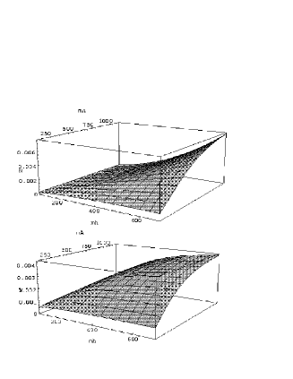
Figure 3: The figure 3 is for the parameter space $(N_{\mu e},m_{h},m_{A})$ for the models (aI) and (aII) respectively. We set $\tan\beta=1$,the higgs mass $m_{H^{0}}=500$ GeV and $\alpha=\pi/16$.

The 3D plots $(N_{\mu e},m_{h},m_{A})$ are shown in the figure 3 for $m_{H}=500$ GeV, $\alpha=\pi/16$ and $\tan\beta=1$. They represent the models (aI) and (aII), similar to the figure 2. Once again, we realize that the behaviour of both models is quite different.

The figure 4 corresponds to the models (aII) and (bII) in which $m_{H^{0}}=300$ GeV and $\alpha=\pi/16.\;$ For the model (aII) we use $\tan\beta=1.\;$ These graphics illustrate that the cases (a) and (b) are substantially different.

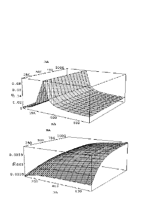
Figure 4: Figure 4 shows the differences between models (a) and (b), it is plotted in the parameter space $(N_{\mu e},m_{h},m_{A})$. The parameter $\tan\beta=1$ for the model (a),the higgs mass $m_{H^{0}}=300$ GeV and $\alpha=\pi/16$.

V Conclusions

In the present work we examine a 2HDM type III which produces FCNC at tree level in the leptonic sector. We classified the model type III according to the VEV taken by the Higgses and to the method used to rotate the mixing matrices. All that, in order to write down the lagrangian in the mass eigenstates. When both doublets acquire a VEV we talk about the case (a), while when only one doublet acquire a VEV we talk about the case (b). On the other hand, when we write $\xi^{D,0},\xi^{U,0}\;$ in terms of $\eta^{D,0},\eta^{U,0}\;$ plus the mass matrices, it is called here a rotation of type I. Where $\xi^{D,0},\xi^{U,0}\;$ are the mixing matrices which couple to $\Phi_{2}\;$ and $\widetilde{\Phi}_{2}\;$ respectively and $\eta^{D,0},\eta^{U,0}\;$ are the FC matrices which couple to $\Phi_{1}\;$and $\widetilde{\Phi}_{1}\;$ respectively. Now, when we solve for $\eta^{D,0},\eta^{U,0}\;$ in terms of $\xi^{D,0},\xi^{U,0}\;$ and the mass matrices we call it a rotation of type II.

In addition, we observe that the 2HDM of type I plus FC interactions is generated by adding the lagrangian of type (a,I) in the up sector and the lagrangian of type (a,I) in the down sector, meanwhile the lagrangian of type II plus FC interactions is generated by adding the lagrangian of type (a,I) in the up sector and the lagrangian of type (a,II) in the down sector. Other two combinations are possible i.e. $\pounds_{Y\left(u\right)}^{\left(a,II\right)}+\pounds_{Y\left(d\right)}^{\left(a,I\right)}$ and $\pounds_{Y\left(u\right)}^{\left(a,II\right)}+\pounds_{Y\left(d\right)}^{\left(a,II\right)}$. Moreover, if we began with a lagrangian of type (a,I) we would obtain the lagrangian (b,I) taking the limit $\tan\beta\rightarrow\infty,\;$ while if we started with a lagrangian of type (a,II) we would obtain the lagrangian (b,II) in the limit $\tan\beta\rightarrow 0$.

To illustrate the importance of this classification we show graphics to find bounds on the FC coupling $N_{\mu e}\;$ coming from the process $\mu\rightarrow e\gamma\;$and we realize that such bounds are sensitive to the type of rotation and also to the structure of the VEV. We also calculate the process $\mu\to 3e$ for both kind of rotations but the constraints obtained were less restrictive than the ones obtained with the process $\mu\to e\gamma$.

Finally, to evaluate such bounds we have used a muon running in the loop for the process $\mu\rightarrow e\gamma\;$instead of a tau as usual. Consequently, we plot the quotient $N_{\mu e}/(N_{\mu\tau}N_{e\tau})\;$in terms of $m_{h^{0}}\;$and $\beta\;$, getting a wide range of allowed values for that quotient, showing that this assumption is reasonable.

We acknowledge to M. Nowakowski for his suggestions and for the careful reading of the manuscript. This work was supported by COLCIENCIAS.

References

• (1) M. Ciuchini, et. al., Phys. Lett. B 316, 127 (1993); Nucl. Phys. B 421, 41 (1994); S. Bertolini, F. Borzumati, A. Masiero and G. Ridolfi, Nucl. Phys. B 353 591 (1991).
• (2) H. Stern and M. K. Gaillard, Ann. Phys. 76, 580 (1973); C. S. Kim, J. L. Rosner and C. P Yuan, Phys. Rev. 42, 96 (1990).
• (3) T. Imami and C. S. Lim, Prog. The. Phys. 65, 297 (1981).
• (4) J. L. Diaz-Cruz, et. al., Phys. Rev. D 41, 891 (1990); G. Eilam, J. Hewett and A. Soni, Phys. Rev D 44, 1473 (1991); G. Couture, C. Hamzanoi and H. Konig, Phys. Rev. D 49, 293 (1995).
• (5) J. L. Hewett and T. Rizzo, Phys. Rep. 183, 193 (1989); G. Baremboim, et. al, Phys. Lett. B 422, 277 (1998); V. Barger, M. Berger and R. Phillips, Phys. Rev. D 52, 1663 (1995); R. Martinez, J.-Alexis Rodriguez and M. Vargas, Phys. Rev. D 60, 077504 (1999); F. del Aguila, J. Aguilar Saavedra and R. Miquel, Phys. Rev. Lett. 82, 1628 (1999).
• (6) J. Liu and L. Wolfenstein, Nucl. Phys. B 289, 1 (1987).
• (7) M. Nowakowski and A. Pilaftsis, Nucl. Phys. B 461, 19 (1996); A. Joshipura and M. Nowakowski, Phys. Rev. D 51, 5271 (1995); G. Ross and J. W. F. Valle, Phys. Lett. B. 151, 375 (1985).
• (8) K. Arisaka, et. al., Phys. Rev. Lett. 70, 1049 (1993).
• (9) K. Arisaka, et. al., Phys. Lett. B. 432, 230 (1993).
• (10) A. M. Lee, et. al., Phys. Rev. Lett. 64, 165 (1990).
• (11) R. D. Bolton, et. al., Phys. Rev. D. 38, 2077 (1983); M. L. Brooks, et. al., Phys. Rev. Lett. 83, 1521 (1999).
• (12) U. Bellgardt et. al., Nucl. Phys. B 299, 1 (1998).
• (13) C. Dohmen et. al. Phys. Lett. B. 317, 631 (1993).
• (14) S. Glashow and S. Weinberg, Phys. Rev. D 15, 1958 (1977).
• (15) Marc Sher and Yao Yuan, Phys. Rev. D 44, 1461 (1991)
• (16) T.P. Cheng and M. Sher, Phys. Rev. D 35, 3490 (1987)
• (17) D. Atwood, L. Reina and A. Soni, Phys. Rev. D 55, 3156 (1997); G: Cvetic, S. S: Hwang and C. S. Kim., Phys. Rev. D 58, 116003 (1998).
• (18) Y. Fukuda, et. al., Phys. Rev. Lett. 81, 1562 (1998)
• (19) A. Kaustubh, M. Graessner Phys. Rev. D 61, 075008 (2000).
• (20) Y. Okada, K. Okumura, Y. Shimizu, Phys. Rev. D. 61, 094001 (2000)
• (21) D. Atwood, L. Reina and A. Soni, Phys. Rev. D. 53, 1199 (1996); Phys. Rev. D. 54, 3296 (1996); Phys. Rev. Lett. 75, 3800 (1993).
• (22) G. Lopez, R. Martinez and G. Munoz, Phys. Rev. D 58, 033003 (1998)
• (23) Marc Sher, hep-ph/0006159v3
• (24) Workshop on Physics at the First Muon Collider and at the Front End of the Muon Collider, ed. S. Geer and R. Raja (AIP Publishing, Batavia Ill 1997)
• (25) W.S. Hou, Phys. Lett B 296, 179 (1992); D. Cahng, W. S. Hou and W. Y. Keung, Phys. Rev. D 48, 217 (1993).
• (26) M. Sher and Y. Yuan, Phys. Rev. D. 44, 1461 (1991).
• (27) S. Nie and M. Sher, Phys. Rev. D. 58, 097701 (1998).
• (28) For a review see J. Gunion, H. Haber, G. Kane and S. Dawson, The Higgs Hunter’s Guide, (Addison-Weslwy, New York, 1990)
• (29) D. Atwood, L. Reina and A. Soni, Phys. Rev. D 55, 3156 (1997); Phys. Rev. Lett. 75, 3800 (1995).
• (30) Shuquan Nie and Marc Sher, hep-ph/9805376