Heavy quark production in $\gamma\gamma$ collisions revisited

Abstract:

Heavy quark production in $\gamma\gamma$ collisions is reanalyzed. It is argued that evaluating the cross section $\sigma(\gamma\gamma\rightarrow Q\overline{Q})$ in a well-defined renormalization scheme requires the inclusion of direct photon contributions up to the order $\alpha^{2}\alpha_{s}^{2}$. The order $\alpha^{2}\alpha_{s}^{2}$ direct photon contributions are furthermore needed for factorization scale invariance of the sum of direct and resolved photon contributions. The importance of quantitative analysis of renormalization and factorization scale dependence of the approximation currently used for the evaluation of $\sigma(\gamma\gamma\rightarrow Q\overline{Q})$ is emphasized as the only way of estimating the theoretical uncertainty related to the ambiguity in choosing these scales.

1 Introduction

Heavy quark production in $\gamma\gamma$ collisions has recently received increased theoretical attention [1, 2, 3] motivated by new experimental data on $c\overline{c}$ and $b\overline{b}$ production from LEP2 [4], which provide particularly suitable framework for the confrontation of perturbative QCD with data. The results obtained so far and shown, for instance, in Fig. 2 of [5] are mixed and inconclusive.

The data on $c\overline{c}$ production coming from different experiments are not mutually quite compatible but all fall into the broad band of theoretical prediction. This is possible because this band reflecting the current uncertainties of theoretical calculations is so broad that it can accommodate results differing by a factor of 2.5! The analogous band narrows somewhat for the $b\overline{b}$ production, but even there the lower and upper range of theoretical predictions differ by a factor of 2. In this case the two data points available are a factor of 3 above the median of theoretical predictions, but the experimental errors are too large to draw any definite conclusions. If confirmed, it would, however, be difficult to accommodate this result theoretically as one expects perturbative QCD to be better applicable to $b\overline{b}$ production than to the $c\overline{c}$ one. In the words of [3] “there is a serious discrepancy with bottom data”.

Theoretical “errors” come in part from the uncertainty in the values of $m_{c}$ and $m_{b}$ but also from the dependence of finite order QCD approximations on the renormalization and factorization scales and schemes. On the experimental side, major part of the error bars reflects the uncertainties in the extrapolation of visible cross section into the full phase space, which can be reduced only if better understanding of the theory is achieved. In such a situation it appears useful and timely to reanalyze the theoretical framework currently used for analyses of heavy quark production in $\gamma\gamma$ collisions, with particular attention to the renormalization and factorization scale invariance. This paper was motivated in part by nontrivial results of the detailed analysis of these dependencies in the case of heavy quark production in pp and $\overline{\mathrm{p}}$p collisions performed in [6]. Using this analysis as guidance, I will discuss the approximation currently used for the evaluation of $\sigma(\gamma\gamma\rightarrow Q\overline{Q})$ and point out its shortcomings. In particular, I will argue that it does not represent genuine next-to-leading order (NLO) QCD approximation and show that the missing ingredient are direct photon contributions of the order $\alpha^{2}\alpha_{s}^{2}$. These terms, which have not yet been calculated, come in three classes, each playing its specific role.

The paper is organized as follows. In the next two sections basic facts relevant for our discussion are recalled and the conventional treatment of $\sigma(\gamma\gamma\rightarrow Q\overline{Q})$ reviewed. In Section 4 two distinct attitudes toward the meaning and content of the terms “leading” and “next-to-leading” orders of QCD are introduced and compared. Direct and resolved photon contributions to $\sigma(\gamma\gamma\rightarrow Q\overline{Q})$ are analyzed in Sections 5 and 6 respectively, followed in Section 7 by the discussion of phenomenological consequences of the present analysis.

2 Basic facts and formulae on the structure of the photon

The factorization scale dependence of parton distribution functions (PDF) of the photon is determined by the system of coupled inhomogeneous evolution equations for quark singlet and nonsinglet and gluon distribution functions

$$\frac{{\mathrm{d}}\Sigma(x,M)}{{\mathrm{d}}\ln M^{2}} = \delta_{\Sigma}k_{q}+P_{qq}\otimes\Sigma+P_{qG}\otimes G,$$ (1)

$$\frac{{\mathrm{d}}G(x,M)}{{\mathrm{d}}\ln M^{2}} = k_{G}+P_{Gq}\otimes\Sigma+P_{GG}\otimes G,$$ (2)

$$\frac{{\mathrm{d}}q_{\mathrm{NS}}(x,M)}{{\mathrm{d}}\ln M^{2}} = \delta_{\mathrm{NS}}k_{q}+P_{\mathrm{NS}}\otimes q_{\mathrm{NS}},$$ (3)

where $\delta_{\mathrm{NS}}\equiv 6n_{f}\left(\langle e^{4}\rangle-\langle e^{2}\rangle^{2}\right)$, $\delta_{\Sigma}=6n_{f}\langle e^{2}\rangle$ and

$$k_{q}(x,M) = \frac{\alpha}{2\pi}\left[k^{(0)}_{q}(x)+\frac{\alpha_{s}(M)}{2\pi}k_{q}^{(1)}(x)+\left(\frac{\alpha_{s}(M)}{2\pi}\right)^{2}k^{(2)}_{q}(x)+\cdots\right],$$ (4)

$$k_{G}(x,M) = \frac{\alpha}{2\pi}\left[~{}~{}~{}~{}~{}~{}~{}~{}~{}~{}~{}~{}\frac{\alpha_{s}(M)}{2\pi}k_{G}^{(1)}(x)+\left(\frac{\alpha_{s}(M)}{2\pi}\right)^{2}k^{(2)}_{G}(x)+\cdots\;\right],$$ (5)

$$P_{ij}(x,M) = ~{}~{}~{}~{}~{}~{}~{}~{}~{}~{}~{}~{}~{}~{}~{}~{}~{}~{}\frac{\alpha_{s}(M)}{2\pi}P^{(0)}_{ij}(x)+\left(\frac{\alpha_{s}(M)}{2\pi}\right)^{2}P_{ij}^{(1)}(x)+\cdots.$$ (6)

The leading order splitting functions $k_{q}^{(0)}(x)=(x^{2}+(1-x)^{2})$ and $P^{(0)}_{ij}(x)$ are unique, while all higher order ones $k^{(j)}_{q},k^{(j)}_{G},P^{(j)}_{kl},j\geq 1$ depend on the choice of the factorization scheme (FS). The equations (1-3) can be recast into evolution equations for $q_{i}(x,M),\overline{q}_{i}(x,M)$ and $G(x,M)$ with inhomogeneous splitting functions $k_{q_{i}}^{(0)}=3e_{i}^{2}k_{q}^{(0)}$. The couplant $\alpha_{s}$ depends on the renormalization scale $\mu$ and satisfies the renormalization group equation

$$\frac{{\mathrm{d}}\alpha_{s}(\mu)}{{\mathrm{d}}\ln\mu^{2}}\equiv\beta(\alpha_{s}(\mu))=-\frac{\beta_{0}}{4\pi}\alpha_{s}^{2}(\mu)-\frac{\beta_{1}}{16\pi^{2}}\alpha_{s}^{3}(\mu)+\cdots,$$ (7)

where, in QCD with $n_{f}$ massless quark flavours, the first two coefficients, $\beta_{0}=11-2n_{f}/3$ and $\beta_{1}=102-38n_{f}/3$, are unique, while all the higher order ones are ambiguous. These non-unique coefficients, together with the boundary condition on the solution of (7), define the so called renormalization scheme (RS). The boundary condition is conveniently specified by the scale parameter $\Lambda_{\mathrm{RS}}$, which depends on the RS and corresponds to such a value of $\mu$ for which $\alpha_{s}(\mu)=\infty$. The couplant $\alpha_{s}$ is thus actually a function of the ratio $\mu/\Lambda_{\mathrm{RS}}$, which behaves for large $\mu$ as $\alpha_{s}(\mu/\Lambda)\approx 4\pi/\beta_{0}\ln(\mu^{2}/\Lambda^{2})$. For the sake of brevity I shall, however, drop the explicit specification of the dependence on the RS and write $\alpha_{s}(\mu)$ only.

Provided perturbative expressions are summed to all orders, the results for physical quantities are independent of both the renormalization scale and scheme, but for any finite order approximation the numerical results do depend on $\mu$ and RS and the consistency of the theory merely requires that their variations with $\mu$ and RS are of higher order of $\alpha_{s}$ than those taken into account. However, as the variation of $\alpha_{s}(\mu)$ with $\mu$ (as well as with the RS) is proportional to $\alpha_{s}^{2}$, we must include at least first two consecutive nonzero powers of $\alpha_{s}$ in perturbative expansions of physical quantities for the necessary cancellation to operate and for the finite order approximation to be performed in a well-defined RS of the couplant $\alpha_{s}$.

Figure 1: Diagrams defining the point-like parts of nonsinglet quark and gluon distribution functions. The resummation involves integration over parton virtualities $\tau\leq M^{2}$ and is represented by the junction of the blob and the $\gamma\rightarrow q\overline{q}$ vertex. Partons going into the hard collision are denoted by $x,\tau$.

Due to the presence of the inhomogeneous splitting functions $k_{q}$ and $k_{G}$ a general solution of the evolution equations (1-3) can be split into the particular solutions of the full inhomogeneous equations and a general solutions, called hadron-like (HAD), of the corresponding homogeneous ones. A subset of the former resulting from the resummation of contributions of diagrams in Fig. 1, describing multiple parton emissions off the primary pure QED vertex $\gamma\rightarrow q\overline{q}$ and vanishing at $M=M_{0}$, are called point-like (PL) solutions. Due to the arbitrariness in the choice of $M_{0}$ the separation of PDF into their point-like and hadron-like parts is, however, ambiguous. In general we can thus write ($D=q,\overline{q},G$) [7]

$$D(x,M)=D^{\mathrm{PL}}(x,M,M_{0})+D^{\mathrm{HAD}}(x,M,M_{0}).$$ (8)

The hadron-like parts can be represented by the same solid blobs as those of hadrons. Appropriate graphical representation of the point-like ones, proposed in [8, 9], is shown in Fig. 1. By joining the primary $\gamma\rightarrow q\overline{q}$ vertex to the solid blob it reflects its perturbative origin.

The different nature of the UV renormalization of QCD quantities, generating the renormalization scale and scheme dependence of $\alpha_{s}$, and IR “renormalization” involved in the definition of PDF represents the main reason for keeping the factorization and renormalization scales $M$ and $\mu$ as independent free parameters. The former sets the upper bound on the virtualities of partons included in the definition of PDF and comes from IR part of loop corrections as well as integrals over real parton emissions. The renormalization scale, on the other hand, defines the lower bound on virtualities included in the renormalized colour charges, masses and fields and comes entirely from loops. There is no compelling theoretical reason why these two scales should be identified [10].

3 $\sigma(\gamma\gamma\rightarrow Q\overline{Q})$: the conventional approach

In [1, 2, 3] the “next–to–leading order” QCD approximation is defined by taking the first two terms in expansions of direct, as well as single and double resolved photon contributions

$$\sigma_{\mathrm{dir}} = \sigma_{\mathrm{dir}}^{(0)}+~{}~{}~{}~{}~{}\sigma_{\mathrm{dir}}^{(1)}\alpha_{s}(\mu)+\sigma_{\mathrm{dir}}^{(2)}(M,\mu)\alpha_{s}^{2}(\mu)+\sigma_{\mathrm{dir}}^{(3)}(M,\mu)\alpha_{s}^{3}(\mu)+\cdots,$$ (9)

$$\sigma_{\mathrm{sr}} = ~{}~{}~{}~{}~{}~{}~{}~{}\sigma_{\mathrm{sr}}^{(1)}(M)\alpha_{s}(\mu)+\sigma_{\mathrm{sr}}^{(2)}(M,\mu)\alpha_{s}^{2}(\mu)+\sigma_{\mathrm{sr}}^{(3)}(M,\mu)\alpha_{s}^{3}(\mu)+\cdots,$$ (10)

$$\sigma_{\mathrm{dr}} = ~{}~{}~{}~{}~{}~{}~{}~{}~{}~{}~{}~{}~{}~{}~{}~{}~{}~{}~{}~{}~{}~{}~{}~{}~{}~{}~{}~{}~{}~{}~{}~{}\sigma_{\mathrm{dr}}^{(2)}(M)\alpha_{s}^{2}(\mu)+\sigma_{\mathrm{dr}}^{(3)}(M,\mu)\alpha_{s}^{3}(\mu)+\cdots$$ (11)

to the total cross section $\sigma(\gamma\gamma\rightarrow Q\overline{Q})$ for the heavy quark pair production in $\gamma\gamma$ collisions

$$\sigma(\gamma\gamma\rightarrow Q\overline{Q})=\sigma_{\mathrm{dir}}+\sigma_{\mathrm{sr}}+\sigma_{\mathrm{dr}}.$$ (12)

In [1, 2, 3] three light quarks ($u,d,s$) were considered as intrinsic for the evaluation of $\sigma(\gamma\gamma\rightarrow c\overline{c})$ and four ($u,d,s,c$) in the case of $b\overline{b}$ production, which is appropriate taking into account that $m_{b}\gg m_{c}$. Although the general strategy of the GRV group is to consider as intrinsic quarks (of both the photon and proton) the light quarks $u,d,s$ only, the GRV set used in [1] parameterizes the effects of heavy quark production far above their thresholds by means of the charm and bottom quark distribution functions and is thus compatible with [1].

Note that while $\sigma_{\mathrm{dir}}^{(0)}$ and $\sigma_{\mathrm{dir}}^{(1)}$ are functions of $s/m_{Q}^{2}$ only, the lowest order single and double resolved photon contributions $\sigma_{\mathrm{sr}}^{(1)}$ and $\sigma_{\mathrm{dr}}^{(2)}$ depend, via PDF of the light quarks and gluons, also on the factorization scale $M$, assumed for simplicity to be the same for both colliding photons. All higher order coefficients in (9-11) depend on both the factorization and renormalization scales $M$ and $\mu$. The lowest order term in (9) comes from pure QED and equals

$$\sigma^{(0)}_{\mathrm{dir}}=\sigma_{0}\left[\left(1+\frac{4m_{Q}^{2}}{s}-\frac{8m_{Q}^{4}}{s^{2}}\right)\ln\frac{1+\beta}{1-\beta}-\beta\left(1+\frac{4m_{Q}^{2}}{s}\right)\right],$$ (13)

where $s$ denotes the square of total $\gamma\gamma$ collision energy, $\beta\equiv\sqrt{1-4m_{Q}^{2}/s}$ and $\sigma_{0}\equiv 12\pi\alpha^{2}e_{Q}^{4}/s$. For the direct photon contribution (9) the renormalization and factorization scales $\mu$ and $M$ appear first in $\sigma_{\mathrm{dir}}^{(2)}$, which, however, is not included in [1, 2, 3].

Defined in this way, the direct, single resolved and double resolved contributions start and end in (9-11) at different powers of $\alpha_{s}$. In the [1, 2, 3] this is justified by claiming that PDF of the photon behave as $\alpha/\alpha_{s}$, and consequently all three expansions (9-11) start and end at the same powers $(\alpha_{s})^{0}=1$ and $\alpha_{s}$, respectively. However, as argued in detail in [11], the logarithm $\ln M^{2}$ characterizing the large $M$ behaviour of PDF of the photon cannot be interpreted as $1/\alpha_{s}(M)$, as it comes from integration over the transverse degree of freedom of the purely QED vertex $\gamma\rightarrow q\overline{q}$! If QCD is switched off by sending, for fixed $M_{0}$, $\Lambda\rightarrow 0$, quark and gluon distribution functions of the photon approach their finite QED expressions

$$q_{i}(x,M)\rightarrow q_{i}^{\mathrm{QED}}(x,M)\equiv\frac{\alpha}{2\pi}3e_{i}^{2}k_{q}^{(0)}(x)\ln\frac{M^{2}}{M_{0}^{2}},~{}~{}~{}~{}~{}~{}G(x,M)\rightarrow G^{\mathrm{QED}}(x,M)=0,$$ (14)

where $M_{0}$ regularizes the parallel singularity coming from the $\gamma\rightarrow q\overline{q}$ vertex by setting the lower limit on the virtuality of the quark or antiquark going to the hard collision. The relation (14) then implies that the single and double resolved photon contributions (10,11) vanish in this limit, because $\alpha_{s}(\mu)$ does so. In the absence of QCD we thus get, as we must, the purely QED result $\sigma_{\mathrm{dir}}^{(0)}$. Had the PDF of the photon really behaved as $\alpha/\alpha_{s}$, we would, on the other hand, expect finite contributions from the lowest order single and double resolved photon contributions (10,11) even in the limit of switching QCD off. I will discuss this limit, together with the large $M$ behaviour of PDF of the photon in detail in subsection 6.1. Taking into account the separation (8) we can distinguish 5 classes of resolved photon contributions:

• Single resolved photon using

  • hadron-like parts of PDF ($\sigma_{\mathrm{srh}}$),

  • point-like parts of PDF ($\sigma_{\mathrm{srp}}$).

• Double resolved photon using

  • hadron-like parts of PDF on both sides ($\sigma_{\mathrm{drhh}}$),

  • hadron-like parts of PDF on one side and point-like ones on the other ($\sigma_{\mathrm{drhp}}$),

  • point-like parts of PDF on both sides ($\sigma_{\mathrm{drpp}}$).

With this subdivision of $\sigma_{\mathrm{sr}}$ and $\sigma_{\mathrm{dr}}$ in mind we can rewrite (12) as follows

$$\sigma(\gamma\gamma\rightarrow Q\overline{Q})=\sigma_{\mathrm{dir}}+\sigma_{\mathrm{srh}}+\sigma_{\mathrm{srp}}+\sigma_{\mathrm{drhh}}+\sigma_{\mathrm{drhp}}+\sigma_{\mathrm{drpp}}.$$ (15)

4 Discourse on semantics: defining LO and NLO in QCD

Although the definition of the concepts “leading-order” (LO) and “next-to-leading-order” (NLO) QCD approximations is primarily a matter of semantics, it is in my view preferable to use the terminology that respects the basic fact that we have in mind orders of QCD, rather than the total number of terms taken into account in expansions (9-11). Counting only the powers of $\alpha_{s}$ will allow us to associate the term “NLO” with calculations performed in a well-defined renormalization scheme of the couplant $\alpha_{s}$ as well as factorization scheme of PDF. In this context it is useful to recall the meaning of theses terms for three physical quantities related to (12).

4.1 $\sigma(\mathrm{e}^{+}\mathrm{e}^{-}\rightarrow{\mathrm{hadrons}})$

For proper treatment of the direct photon contribution $\sigma_{\mathrm{dir}}$ in (9), the total cross section for e⁺e^- annihilations into hadrons at the cms energy $Q$ provides particularly suitable guidance. For $n_{f}$ effectively massless quark flavors we have

$$\sigma_{\mathrm{had}}(Q)=\sigma_{\mathrm{had}}^{(0)}(Q)+\alpha_{s}(\mu)\sigma_{\mathrm{had}}^{(1)}(Q)+\alpha_{s}^{2}(\mu)\sigma_{\mathrm{had}}^{(2)}(Q/\mu)+\cdots=\sigma_{\mathrm{had}}^{(0)}(Q)(1+r(Q)),$$ (16)

where the lowest order term $\sigma_{\mathrm{had}}^{(0)}(Q)\equiv(4\pi\alpha^{2}/Q^{2})\sum_{f}e_{f}^{2}$ comes, similarly as $\sigma_{\mathrm{dir}}^{(0)}$ in (9), from pure QED, namely the diagram in Fig. 2a, whereas genuine QCD effects are contained in

$$r(Q)=\frac{\alpha_{s}(\mu)}{\pi}\left[1+\frac{\alpha_{s}(\mu)}{\pi}r_{1}(Q/\mu)+\cdots\right].$$ (17)

The lowest order contribution to $r(Q)$ results from the sum of the integral over the cross section for real gluon emissions (Fig. 2b) with the interference term between the basic QED diagram of Fig. 2a and one loop corrections to it, shown in Fig. 2c. The next-to-lowest order contribution to (17), $(\alpha_{s}/\pi)^{2}r_{1}$, results from summing the integral over the double parton emissions, exemplified by the diagrams in Fig. 2d, with the integral over the interference term between single gluon emission (Fig. 2b) and one loop corrections to it (for examples see Fig. 2e), and the interference term between the QED contribution of Fig. 2a and the two loop corrections to it (not shown). At each order of $\alpha_{s}$ the finiteness of the sum is guaranteed by the KLN theorem.

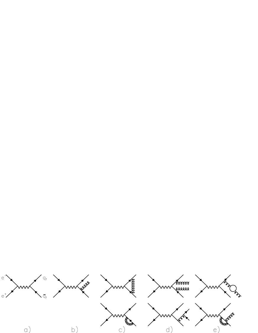
Figure 2: Feynman diagrams contributing to the cross section $\sigma_{\mathrm{ee}}(Q)$ up to the order $\alpha^{2}\alpha_{s}^{2}$. Diagrams with real gluon emissions off and loop corrections on the upper quark leg are understood to be included.

For the quantity (16) nobody calls the lowest order term $\sigma_{\mathrm{had}}^{(0)}(Q)$ the “leading-order” and the next one, i.e. $\sigma_{\mathrm{had}}^{(0)}(Q)\alpha_{s}(\mu)/\pi$, the “next–to–leading order” QCD approximations, but these terms are applied to genuine QCD effects contained in $r(Q)$. To work in a well-defined renormalization scheme of $\alpha_{s}$ requires including in (17) at least first two consecutive nonzero powers of $\alpha_{s}(\mu)$, because only the coefficient $r_{1}(Q/\mu)/\pi^{2}$ standing by $\alpha_{s}^{2}$ depends on the renormalization scale and scheme. The renormalization scale invariance of the NLO approximation to $\sigma_{\mathrm{had}}(Q)$ implies that the implicit $\mu$-dependence of the leading order term $\alpha_{s}(\mu)/\pi$ in (17) is cancelled to order $\alpha_{s}^{2}$ by explicit $\mu$-dependence of the coefficient $r_{1}(Q/\mu)/\pi^{2}$. The $\ln\mu^{2}$ term necessary for this cancellation comes from loop corrections described by diagrams like those in Fig. 2e. Note that the loops in Fig. 2c contribute to the renormalization of $\alpha$, rather than of $\alpha_{s}$. Because $\alpha_{s}(\mu)$ is a monotonous function of $\mu$ spanning the whole interval $(0,\infty)$, the inclusion of first two consecutive nonzero powers of $\alpha_{s}$ is also a prerequisite for the applicability of any of the scale fixing methods [12, 13, 14] available on the market. Without it, there is no preferred scale and, consequently, the LO QCD approximations become entirely arbitrary.

For purely perturbative quantities the association of the term “NLO QCD approximation” with a well-defined renormalization scheme is a generally accepted convention, in my view worth retaining for physical quantities in any hard scattering process.

4.2 $F_{2}^{\mathrm{p}}(x,Q^{2})$

For physical quantities involving PDF proper definition of the terms “leading” and “next-to-leading” order concerns beside the renormalization scale and scheme of $\alpha_{s}$ also the factorization scale and scheme of these PDF.

For proton the structure functions $F_{2}^{\mathrm{p}}(x,Q^{2})$ is given as the convolution of PDF with the corresponding coefficient functions. Dropping for simplicity quark charges we generically have

$$F_{2}^{\mathrm{p}}(x,Q^{2})=q(M)\otimes C_{q}(Q/M)+G(M)\otimes G_{G}(Q/M),$$ (18)

where quark and gluon distribution functions satisfy the homogeneous evolution equations and

$$C_{q}(x,Q/M) = \delta(1-x)+\frac{\alpha_{s}(\mu)}{2\pi}C_{q}^{(1)}(x,Q/M)+\left(\frac{\alpha_{s}(\mu)}{2\pi}\right)^{2}C_{q}^{(2)}(x,Q/M,Q/\mu)+\cdots$$ (19)

$$C_{G}(x,Q/M) = 0~{}~{}~{}~{}~{}~{}~{}~{}~{}+\frac{\alpha_{s}(\mu)}{2\pi}C_{G}^{(1)}(x,Q/M)+\left(\frac{\alpha_{s}(\mu)}{2\pi}\right)^{2}C_{G}^{(2)}(x,Q/M,Q/\mu)+\cdots.$$ (20)

The standard definition of LO QCD approximation to $F_{2}^{\mathrm{p}}(x,Q^{2})$ amounts to setting

$$F_{2,{\mathrm{LO}}}^{\mathrm{p}}(x,Q^{2})=q(x,M),$$ (21)

where $M\propto Q$ and $q(x,M)$ satisfy (1- 3) with $P_{ij}^{(0)}$ on their r.h.s. only. At the NLO the terms proportional to $P_{ij}^{(1)},C_{q}^{(1)}$ and $C_{G}^{(1)}$ are included as well. All these functions depend on the factorization scheme, and the latter two also on $M$, and must therefore be included in any analysis which aims at working in a well-defined such scheme. Although $F_{2,{\mathrm{LO}}}^{\mathrm{p}}(x,Q^{2})$ involves only the first, purely QED term in (19), it describes QCD effects, because they drive the $M$-dependence of $q(x,M)$. At the NLO, the factorization scale dependence of $q(x,M)$ in (18) is cancelled by the explicit $M$-dependence of the coefficient $C_{q}^{(1)}(Q/M)$, similarly as renormalization scale dependence of $\alpha_{s}(\mu)$ in the first term of (17) is cancelled to the order $\alpha_{s}^{2}$ by the $\mu$-dependence of the coefficient $r_{1}(Q/\mu)$. The standard definitions of LO and NLO approximations for $F^{\mathrm{p}}_{2}(x,Q^{2})$ thus conform to the basic requirement that the term “leading order” describes the lowest order contribution affected by QCD effects and that working in a well-defined renormalization as well as factorization schemes requires at least the next-to-leading order approximation.

4.3 $F_{2}^{\gamma}(x,Q^{2})$

The conventional analysis of photon structure function employs the same definition of the terms “leading” and “next-to-leading” orders as that used in [1, 2, 3]. I have discussed its shortcomings in [11] and will therefore merely recall the main points relevant for this paper. For the real photon $F_{2}^{\gamma}(x,Q^{2})$ is given as the sum of convolutions

$$\frac{1}{x}F_{2}^{\gamma}(x,Q^{2}) = q_{\mathrm{NS}}(M)\otimes C_{q}(Q/M)+\frac{\alpha}{2\pi}\delta_{\mathrm{NS}}C_{\gamma}+$$ (22)

$$\langle e^{2}\rangle\Sigma(M)\otimes C_{q}(Q/M)+\frac{\alpha}{2\pi}\langle e^{2}\rangle\delta_{\Sigma}C_{\gamma}+\langle e^{2}\rangle G(M)\otimes C_{G}(Q/M)$$

of PDF of the photon with the coefficient functions $C_{q}$ and $C_{G}$, given in (19-20), and

$$C_{\gamma}(x,Q/M)=C_{\gamma}^{(0)}(x,Q/M)+\frac{\alpha_{s}(\mu)}{2\pi}C_{\gamma}^{(1)}(x,Q/M)+\left(\frac{\alpha_{s}(\mu)}{2\pi}\right)^{2}C_{\gamma}^{(1)}(x,Q/M)+\cdots,$$ (23)

where the lowest order term in (23)

$$C_{\gamma}^{(0)}(x,Q/M)=\left(x^{2}+(1-x)^{2}\right)\left[\ln\frac{M^{2}}{Q^{2}}+\ln\frac{1-x}{x}\right]+8x(1-x)-1$$ (24)

comes, similarly as $k_{q}^{(0)}$ in (4) and $\sigma_{\mathrm{had}}^{(0)}$ in (16), from pure QED. Throughout this subsection I will discuss only the point-like part of $F_{2}^{\gamma}(x,Q^{2})$, which is related to the point-like parts of PDF of the photon. The QED contribution to $F_{2}^{\gamma}(x,Q^{2})$

$$\frac{1}{x}F_{2}^{\gamma,\mathrm{QED}}(x,Q^{2})=\sum_{i=1}^{n_{f}}e_{i}^{2}\left(q_{i}^{\mathrm{QED}}(x,M)+\overline{q}_{i}^{\mathrm{QED}}(x,M)\right)+\frac{\alpha}{2\pi}6n_{f}\langle e^{4}\rangle C_{\gamma}^{(0)}(x,Q/M)$$ (25)

comes from the diagram in Fig. 3a and is actually independent of $M$ because the $M$-dependence of $q_{i}^{\mathrm{QED}}(x,M)$ is cancelled by that of $C_{\gamma}^{(0)}(x,Q/M)$. Switching on QCD implies that terms proportional to nonzero powers of $\alpha_{s}$ in the splitting as well as coefficient functions (4-6) and (19,20,23) are taken into account.

Figure 3: Examples of diagrams contributing to $F_{2}^{\gamma}$ in QED (a), ${\cal O}(\alpha_{s})$ (b-c) and ${\cal O}(\alpha_{s}^{2})$ (d-i) QCD.

It appears natural to define as the leading order QCD approximation to $F_{2}^{\gamma}$ the one that takes into account those of the above terms proportional to $\alpha_{s}$ which contribute to the ${\cal O}(\alpha_{s})$ correction to (25). These are $k_{q}^{(1)}$ and $P_{ij}^{(0)}$ in (4-6) and $C_{q}^{(1)}$ and $C_{\gamma}^{(1)}$ in (19) and (23). The remaining ${\cal O}(\alpha_{s})$ terms, $k_{G}^{(1)}$ and $C_{G}^{(1)}$, do not contribute to $\alpha_{s}$ correction to $F_{2}^{\gamma}$ because $G^{\mathrm{QED}}(x,M)=0$. The functions $k_{q}^{(1)},~{}C_{q}^{(1)}$ as well as $C_{\gamma}^{(1)}$ result from evaluation of the order $\alpha^{2}\alpha_{s}$ diagrams , exemplified by those in Fig. 3b,c. It is worth emphasizing that despite the presence of loops involving gluons, no renormalization of $\alpha_{s}$ is performed at this order, because the loops, like that in Fig. 3b, contribute to the UV renormalization of $\alpha$, not $\alpha_{s}$! In this definition the LO QCD approximation to $F_{2}^{\gamma}$ thus involves (see [11] for explicit formula) in addition to the purely QED quantities $k_{q}^{(0)}$ and $C_{\gamma}^{(0)}$ also $k_{q}^{(1)},P_{ij}^{(0)},C_{q}^{(1)}$ and $C_{\gamma}^{(1)}$. Note that the conventional LO approximation takes into account out of these 6 quantities only two of them: $k_{q}^{(0)}$ and $P_{ij}^{(0)}$.

According to the approach advocated in [11], the next-to-leading order QCD approximation to $F_{2}^{\gamma}$ includes in addition to the quantities mentioned above also the splitting and coefficient functions proportional to $\alpha_{s}^{2}$, i.e. $k_{q}^{(2)},P_{ij}^{(1)},C_{q}^{(2)},C_{\gamma}^{(2)}$ and takes into account also the contribution generated by the gluonic splitting and coefficient functions $k_{G}^{(1)}$ and $C_{G}^{(1)}$. The evaluation of these quantities involves order $\alpha^{2}\alpha_{s}^{2}$ diagrams, exemplified by those in Fig. 3d-i. These include loop corrections to the LO diagrams (like those in Fig. 3e-g) as well as two parton emissions, exemplified by diagrams in Fig. 3d,h-i. At this order the renormalization of $\alpha_{s}$ starts to operate by removing the UV divergencies coming from loops in Fig. 3e-g (and others). Note that the conventional NLO approximation to $F_{2}^{\gamma}$ (see, for instance, [15]) includes $k_{q}^{(0)},k_{q}^{(1)},P_{ij}^{(0)},P_{ij}^{(1)},C_{\gamma}^{(0)}$ and $C_{q}^{(1)}$, but not $k_{q}^{(2)},C_{q}^{(2)},C_{\gamma}^{(1)},C_{\gamma}^{(2)}$. This is particularly intriguing in the case of the coefficient function $C_{\gamma}^{(1)}$ which stands in (23) by power $\alpha\alpha_{s}$ and is actually known! As $k_{q}^{(2)},C_{q}^{(2)},C_{G}^{(1)}$ and $C_{\gamma}^{(2)}$, have not yet been calculated, a complete NLO QCD approximation of $F_{2}^{\gamma}$ defined in the sense advocated in [11], cannot at the moment be constructed.

The fact that contrary to the case of $F_{2}^{\gamma}$, $C_{q}^{(1)}$ enters $F_{2}^{\mathrm{p}}$ first at the NLO is due to the fact that there is no point-like, perturbatively calculable coupling of the proton to quarks (or gluons) that would generate the inhomogeneous splitting function analogous to $k_{q}^{(0)}$, and thus the pure QED contribution analogous to (14).

5 Direct photon contribution to $\sigma(\gamma\gamma\rightarrow Q\overline{Q})$

In [1, 2, 3] the purely QED contribution $\sigma_{\mathrm{dir}}^{(0)}$ is considered as the leading-order and the sum

$$\sigma_{\mathrm{dir}}^{\mathrm{(01)}}\equiv\sigma_{\mathrm{dir}}^{(0)}+\alpha_{s}(\mu)\sigma_{\mathrm{dir}}^{(1)}$$ (26)

as the NLO approximation of the direct photon contribution $\sigma_{\mathrm{dir}}$. Note that (26) is of the same form as the sum of first two terms in (16) and $\alpha_{s}(\mu)$ is thus the only place where $\mu$ appears. Consequently, $\sigma^{(01)}_{\mathrm{dir}}$ cannot be associated to a well-defined renormalization scheme of $\alpha_{s}$ and therefore does not deserve the label “NLO” even if the NLO expression for $\alpha_{s}(\mu)$ is used therein. For QCD analysis of $\sigma_{\mathrm{dir}}$ in a well-defined renormalization scheme the incorporation of the third term in (9), proportional to $\alpha^{2}\alpha_{s}^{2}$, is indispensable. We need in particular the diagrams like those in Fig. 4j-k, which involve loops contributing to the renormalization of $\alpha_{s}$. The regular, $\mu$-dependent part of their contributions provides the $\ln\mu^{2}$ term canceling the $\mu$ dependence of $\alpha_{s}(\mu)$ in the second term of (26).

Figure 4: Examples of diagrams contributing to $\sigma_{\mathrm{dir}}$ in QED (a), leading (b-d) and next-to-leading (e-l) orders of QCD. Heavy quark are denoted by dashed, light quarks by solid lines.

At the order $\alpha^{2}\alpha_{s}^{2}$ diagrams with light quarks appear as well and we therefore distinguish three classes of contributions, differing by the charge factor $CF$ ($e_{Q}$ and $e_{q}$ denoting charges of heavy and light quarks respectively):

Class A: $CF=e_{Q}^{4}$. Comes from diagrams in which both primary photons couple to heavy quarks or antiquarks. The diagrams of this class may, as those in Fig. 4i-j, contain also light quarks. As emphasized above the diagrams containing loops, like those in Fig. 4j-k, are vital for the renormalization of $\alpha_{s}$. Despite the presence of mass singularities of individual diagrams coming from gluons and light quarks in the final state and loops, the KLN theorem guarantees that at each order of $\alpha_{s}$ the sum of all contributions of this class to $\sigma_{\mathrm{dir}}$ is finite.

Class B: $CF=e_{Q}^{2}e_{q}^{2}$. Comes from diagrams in which one of the primary photons couples to a heavy and the other to a light quark-antiquark pair, like that in Fig. 4h. For massless light quarks this diagram has initial state mass singularity, coming from the region of vanishing light quark virtuality $\tau_{q}$, which is removed by introducing the concept of the resolved photon. This implies subtracting from the corresponding cross section the integral over the double pole $1/(\tau_{q}\tau_{G})$ and putting it into the point-like part of the gluon distribution function appearing in the lowest order single resolved photon diagram of Fig. 5a. Similarly, the single pole term $1/\tau_{q}$ is subtracted and put into the light quark distribution function entering the next-to-lowest order single resolved photon diagram if Fig. 5c.

Class C: $CF=e_{q}^{4}$. Comes from diagrams in which both photons couple to light $q\overline{q}$ pairs, as those in Fig. 4l. In this case the analogous subtraction procedure relates it to the lowest order double resolved photon contribution of the diagram in Fig. 5h.

Because of different charge factors, the classes A, B and C do not mix under renormalization of $\alpha_{s}$ and factorization of mass singularities. Such mixing does, however, occur, within each of these classes. At the order $\alpha^{2}\alpha_{s}^{2}$ all three classes of contributions are needed for theoretical consistency, albeit each for different reason. The class A is needed if the calculation is to be performed in a well-defined RS. In the next Section we shall see that classes B and C must be taken into account for factorization scale invariance of the sum (12) of direct and resolved photon contributions.

6 Resolved photon contribution to $\sigma(\gamma\gamma\rightarrow Q\overline{Q})$

Because the factorization mechanism plays crucial role in my arguments let me recall how it works for heavy quark production in $\overline{\mathrm{p}}$p collisions, where the NLO approximation for $\sigma({\overline{\mathrm{p}}\mathrm{p}}\rightarrow Q\overline{Q})$ involves convolutions of PDF with partonic cross sections up to the order $\alpha_{s}^{3}$. Schematically

$$\sigma^{\mathrm{NLO}}(\overline{\mathrm{p}}\mathrm{p}\rightarrow Q\overline{Q})=D_{1}(M)\otimes\left[\alpha_{s}^{2}(\mu)\sigma^{(2)}+\alpha_{s}^{3}(\mu)\sigma^{(3)}(M,\mu)\right]\otimes D_{2}(M),$$ (27)

where PDF $D_{1}(M)$ and $D_{2}(M)$ of the colliding protons satisfy the homogeneous evolution equations with first two terms in (6) taken into account. Factorization scale invariance of (27) is guaranteed by the fact that the $M$-dependence of $D_{1}(M)$ and $D_{2}(M)$ in the lowest order term of (27) is cancelled to the order considered by the $M$-dependence of $\sigma^{(3)}(M,\mu)$. Graphical representation of this cancellation mechanism exploits the fact that the homogeneous part of the evolution equations (1-3) relate by what I call homogeneous factorization a given diagram with partonic cross section at the order $\alpha_{s}^{2}$ with two diagrams (with incoming quark and gluon respectively) at the order $\alpha_{s}^{3}$ and higher. For the NLO approximation (27) only the lowest order splitting functions $P_{ij}^{(0)}$ appear in this cancellation.

In [6] detailed analysis of the renormalization and factorization scale dependence of (27) has been performed under the assumption $\mu=M$. The results, summarized in Figs. 13-15 of [6], show that the sensitivity of $\sigma^{\mathrm{NLO}}(\overline{\mathrm{p}}\mathrm{p}\rightarrow Q\overline{Q})$ to the variation of $M$ depends sensitively on the ratio $\sqrt{s}/m_{Q}$, as well as on PDF of colliding particles. They also demonstrate that contrary to the traditional expectation the NLO QCD approximation is not necessarily less dependent on the factorization scale $M$ than the LO ones! Whereas at $\sqrt{s}=62$ GeV $\sigma^{\mathrm{NLO}}(\overline{\mathrm{p}}\mathrm{p}\rightarrow b\overline{b})$ is a weaker function of $M$ than $\sigma^{\mathrm{LO}}(\overline{\mathrm{p}}\mathrm{p}\rightarrow b\overline{b})$, and has even a stationary point, this is not true at $\sqrt{s}=630$ GeV. There the NLO prediction is a monotonous function of $M$, which is even steeper than the LO one! Similar lesson follows from comparing different processes at the same energy: whereas $\sigma^{\mathrm{NLO}}(\overline{\mathrm{p}}\mathrm{p}\rightarrow b\overline{b})$ has, as mentioned, a stationary point for $\sqrt{s}=62$ GeV, $\sigma^{\mathrm{NLO}}(\mathrm{p}\mathrm{p}\rightarrow b\overline{b})$ is again a monotonous function of $M$. To assess the stability of QCD calculations of $\sigma(\gamma\gamma\rightarrow Q\overline{Q})$, quantitative analysis of their factorization and renormalization scale dependence along the lines of [6] would be very helpful, better still with $\mu$ and $M$ treated as separate free parameters.

6.1 Single resolved photon: the point-like part

For the point-like part of PDF of the photon the presence of the inhomogeneous splitting function $k_{q}^{(0)}$ in the evolution equations (1,3) implies additional relation, which I call inhomogeneous factorization, to distinguish it from the homogeneous one introduced above, which corresponds to $P^{(0)}_{ij}$. For instance, the lowest order single resolved photon diagram of Fig. 5a is related by homogeneous factorization to the single resolved photon diagram of Fig. 5c. Both of these diagrams are included in the approximation

$$\sigma_{\mathrm{srp}}^{(12)}(M,\mu)\equiv\sigma_{\mathrm{srp}}^{(1)}(M)\alpha_{s}(\mu)+\sigma_{\mathrm{srp}}^{(2)}(M,\mu)\alpha_{s}^{2}(\mu)$$ (28)

employed in [1, 2, 3]. The latter diagram is related via the inhomogeneous factorization to the direct photon diagram of Fig. 5b, which is of the order $\alpha^{2}\alpha_{s}^{2}$ and thus is not included in the approximation (26) of $\sigma_{\mathrm{dir}}$.

Figure 5: Some of Feynman diagrams contributing to $\sigma_{\mathrm{srp}}$ in the leading (a) and next-to-leading (c-f) orders of QCD, together with the related direct photon diagrams of the order $\alpha^{2}\alpha_{s}^{2}$ (b,g) and lowest order double resolved photon diagram (h).

The inhomogeneous factorization, which connects direct and resolved photon diagrams at the same order of $\alpha_{s}$, has a simple interpretation, reflecting its role in removing the mass singularities of direct photon contributions associated with the point-like coupling of initial photons to light quarks. For the direct photon diagram in Fig. 5b (which coincides with the diagram in Fig. 4f) this procedure has been outlined already in Section 5. Let me recall that its finite, $M$-dependent part contributes to class B part of $\sigma_{\mathrm{dir}}^{(2)}$ and cancels the dominant part of the factorization scale dependence of single resolved photon diagram in Fig. 5c. The inclusion of class B direct photon contributions of the order $\alpha^{2}\alpha_{s}^{2}$ is thus vital for factorization scale invariance of the sum (12) of direct and resolved photon contributions. In similar way, the factorization scale invariance implies that single resolved photon diagram of Fig. 5f must be considered together with class C direct photon diagram of the order $\alpha^{2}\alpha_{s}^{2}$, shown in Fig. 5g. This diagram is in turn related by inhomogeneous factorization to the point-like part of lowest order double resolved photon diagram of Fig. 5h, which is of the same order $\alpha^{2}\alpha_{s}^{2}$ and will be discussed below. These considerations apparently contradict the statement in [1]

In contrast to heavy-quark production in hadron collisions we expect small variation of the resolved-$\gamma$ cross section with $\mu$ at the Born level, since the $\mu$ fall off of the parton cross section $[\sim\alpha_{s}^{k}(\mu)]$ is neutralized asymptotically by the increasing number of gluon and quark partons in the photons $\sim[\alpha_{s}^{-1}(\mu)]^{k},~{}k=1$ or $k=2$ for $1$- or $2$-resolved $\gamma$.

I will now argue that the asymptotic behaviour of Born terms in the resolved photon contributions, mentioned in the above quotation, does not actually imply factorization scale invariance of the approximation used in [1, 2, 3]. The large $M$ behaviour of the solutions of the evolution equation (1-3) is the same for all three PDF and reads (in momentum space)

$$q_{\mathrm{NS}}(n,M) = \frac{\alpha}{2\pi}\delta_{\mathrm{NS}}k_{q}^{(0)}(n)\left[\frac{1}{1-\overline{P}_{qq}(n)}\right]\ln M^{2},$$ (29)

$$\Sigma(n,M) = \frac{\alpha}{2\pi}\delta_{\Sigma}k_{q}^{(0)}(n)~{}\left[\frac{1-\overline{P}_{GG}(n)}{(1-\overline{P}_{qq}(n))(1-\overline{P}_{GG}(n))-\overline{P}_{qG}(n)\overline{P}_{Gq}(n)}\right]\ln M^{2},$$ (30)

$$G(n,M) = \frac{\alpha}{2\pi}\delta_{\Sigma}k_{q}^{(0)}(n)~{}\left[\frac{\overline{P}_{Gq}(n)}{(1-\overline{P}_{qq}(n))(1-\overline{P}_{GG}(n))-\overline{P}_{qG}(n)\overline{P}_{Gq}(n)}\right]\ln M^{2},$$

$$= \Sigma(n,M)\frac{\overline{P}_{Gq}(n)}{1-\overline{P}_{GG}(n)}$$

where $\overline{P}_{ij}(n)\equiv 2P^{(0)}_{ij}(n)/\beta_{0}$. Although gluons must be radiated off the primary quarks, which costs powers of $\alpha_{s}$, the $\ln M^{2}$ rise of point-like part of quark distribution function drives the logarithmic rise of $G(n,M)$ as well. Consequently, $\sigma^{(1)}_{\mathrm{srp}}(M)\alpha_{s}(M)$, the lowest order term in (28) (where we set $\mu=M$) approaches at large $M$ a constant, whereas in hadronic collisions the first term in (27) vanishes as $M\rightarrow\infty$. This difference might seem important, but actually is not, because the factorization scale invariance concerns the variation of finite order approximations with $M$, not their magnitude! Moreover, the values of $M$ used in [1], i.e. $M=\sqrt{2}m_{Q}$ is far from asymptotic in any case.

The relations (29-6.1) determine the asymptotic behaviour of PDF of the photon for fixed value of the QCD parameter $\Lambda$. The claim that PDF of the photon behave as $\alpha/\alpha_{s}(M)$ must therefore be interpreted merely as a shorthand for this large $M$ behaviour at fixed $\Lambda$. Interpreting $\ln M^{2}$ as $\ln M^{2}/\Lambda^{2}\propto\alpha_{s}(M)$, would lead us to obviously wrong conclusion that PDF of the photon blow up to infinity when we switch QCD off by sending $\Lambda\rightarrow 0$! On the other hand, as (29-6.1) do not explicitly contain $\Lambda$, they seem to hold for any value of $\Lambda$ and, consequently, one might be tempted to conclude that they survive the limit $\Lambda\rightarrow 0$ as well. That, however, is not the case.

To find what happens with the asymptotics (29-6.1) when we switch QCD off we must reverse the order of limits and first send $\Lambda\rightarrow 0$ for fixed finite $M_{0}$ and $M$. Doing this we get, of course, the pure QED formulae (14), which differ dramatically for the gluon and quantitatively (i.e. by the presence of the square brackets in (29-30) also for the quark distribution functions. The corresponding asymptotic behavior of quark and gluon distribution functions, can be obtained formally also directly from (29-6.1) by sending $\beta_{0}\rightarrow\infty$, which implies setting $\overline{P}_{ij}=0,\forall i,j$ there. This reflects the fact that the factor $2/\beta_{0}$ multiplying in (29-6.1) all the splitting functions $P^{(0)}_{ij}$ results from the following limit

$$\lim_{M\rightarrow\infty}\frac{\alpha_{s}(M)}{2\pi}\ln M^{2}=\frac{2}{\beta_{0}}\lim_{M\rightarrow\infty}\frac{\ln M^{2}}{\ln(M^{2}/\Lambda^{2})}=\frac{2}{\beta_{0}}.$$ (32)

Sending $\alpha_{s}\rightarrow 0$ for fixed $M$ can be achieved either by sending $\Lambda\rightarrow 0$ for fixed finite $M$, or, formally, for any $M$ by sending $\beta_{0}\rightarrow\infty$. The latter option is applicable even for the asymptotics (29-6.1). Clearly, the order of the limits $\Lambda\rightarrow 0$ and $M\rightarrow\infty$ matters.

There is also a second difference between $Q\overline{Q}$ production in pp and $\gamma\gamma$ collisions. At the NLO the $q^{\mathrm{PL}}$ contributes (see diagram in Fig. 5c) to the second term in (28), as it does the quark distribution functions of the proton to the second term in (27). But whereas in the latter case the variation of this term with $M$ is of one order of $\alpha_{s}$ higher than that taken into account in (27), for $\gamma\gamma$ collisions the presence of $k_{q}^{(0)}$ implies that the variation of $\sigma_{\mathrm{srp}}^{(2)}\alpha_{s}^{2}(M)$ with $M$ is of the same order as this contribution itself. As argued above, the cancellation of this dependence requires the inclusion of direct photon contributions of class B and order $\alpha^{2}\alpha_{s}^{2}$.

In summary, the approximation $\sigma_{\mathrm{srp}}^{(12)}(M,\mu)$ defined in (28) has the properties of genuine NLO QCD approximation with respect to the renormalization of $\alpha_{s}$, but without the inclusion of direct photon contributions of classes B and C, like those in Fig. 5b,g, it is not factorization scale invariant to the order considered.

6.2 Single resolved photon: the hadron-like part

This part of $\sigma(\gamma\gamma\rightarrow Q\overline{Q})$ has the same structure as the direct photon contribution to the cross section for heavy quark production in $\gamma$p collisions and I will therefore discuss the main features of the approximation

$$\sigma_{\mathrm{srh}}^{(12)}(M,\mu)\equiv\sigma_{\mathrm{srh}}^{(1)}(M)\alpha_{s}(\mu)+\sigma_{\mathrm{srh}}^{(2)}(M,\mu)\alpha_{s}^{2}(\mu).$$ (33)

in the next subsection together with those of $\sigma_{\mathrm{drhp}}^{(23)}$, which plays the role of the resolved photon contribution in $\gamma$p collisions.

6.3 Double resolved photon: the hadron-like–point-like part

This part of double resolved photon contribution used in [1, 2, 3]

$$\sigma_{\mathrm{drhp}}^{(23)}(M,\mu)\equiv\sigma_{\mathrm{drhp}}^{(2)}(M)\alpha_{s}^{2}(\mu)+\sigma_{\mathrm{drhp}}^{(3)}(M,\mu)\alpha_{s}^{3}(\mu)$$ (34)

has the same properties as the point-like part of resolved photon contribution to $\sigma(\gamma{\mathrm{p}}\rightarrow Q\overline{Q})$. In fact, only the first term in (34) needs to be included in the sum

$$\sigma_{\mathrm{srh}}^{(12)}(M,\mu)+\sigma_{\mathrm{drhp}}^{(23)}(M,\mu)$$ (35)

to make it complete NLO QCD approximation as far as both the renormalization of $\alpha_{s}$ and the definition of PDF of the photon are concerned. Note that the $M$-dependence of $\sigma^{(2)}_{\mathrm{drhp}}(M,\mu)$ induced by the inhomogeneous splitting function $k_{q}^{(0)}$ compensates the $M$-dependence of the part of $\sigma^{(2)}_{\mathrm{srh}}(M,\mu)$ that remains after the subtraction of the singular term coming from the vertex $\gamma\rightarrow q\overline{q}$.

6.4 Double resolved photon: the hadron-like–hadron-like part

This part of double resolved photon contribution has the same structure and properties as (27) and, consequently, the sum of first two terms in (11)

$$\sigma_{\mathrm{drhh}}^{(23)}(M,\mu)\equiv\sigma_{\mathrm{drhh}}^{(2)}(M)\alpha_{s}^{2}(\mu)+\sigma_{\mathrm{drhh}}^{(3)}(M,\mu)\alpha_{s}^{3}(\mu)$$ (36)

has all the features of genuine NLO QCD approximation, both as far as the renormalization of $\alpha_{s}$ and the definition of PDF are concerned.

6.5 Double resolved photon: the point-like–point-like part

The lowest order contribution to this part of $\sigma(\gamma\gamma\rightarrow Q\overline{Q})$ comes from the convolution of point-like parts of PDF of both photons with $\alpha_{s}^{2}$ cross sections of $q\overline{q}\rightarrow Q\overline{Q}$ (see Fig. 5h) and $GG\rightarrow Q\overline{Q}$ (not shown) partonic subprocesses. The former contribution is needed to render the point-like part of single resolved photon contribution (28) coming from the diagram in Fig. 5f factorization scale invariant. But as argued in subsection 6.1, the diagram in Fig. 5h alone is not sufficient for this purpose and class C direct photon diagram of Fig. 5g must be included as well. For the double resolved photon contribution the same diagram is needed for theoretical consistency already at the lowest order, i.e. for the cancellation of part of the $M$-dependence of $\sigma_{\mathrm{drpp}}^{(2)}(M,\mu)\alpha_{s}(\mu)$.

7 Phenomenological consequences

In the preceding sections I have shown that the approximation used in [1, 2, 3]

$$\sigma^{\mathrm{DKF}}(M,\mu)\equiv\sigma_{\mathrm{dir}}^{(01)}(\mu)+\sigma_{\mathrm{sr}}^{(12)}(M,\mu)+\sigma_{\mathrm{dr}}^{(23)}(M,\mu),$$ (37)

based on the sum of first two term in each of the expansions (9-11), does not represent genuine NLO QCD approximation despite the fact that it contains partonic cross sections up to order $\alpha_{s}^{3}$ and uses the NLO form of $\alpha_{s}(\mu)$. The missing direct photon contributions of the order $\alpha^{2}\alpha_{s}^{2}$ come in three classes, which differ by the overall charge factor, reflecting the presence or absence of light quark pairs and the way they couple to the primary photons. Each of these three classes is needed for different reason, but all are needed to make the expression

$$\sigma^{\mathrm{NLO}}(M,\mu)\equiv\sigma_{\mathrm{dir}}^{(02)}(M,\mu)+\sigma_{\mathrm{sr}}^{(12)}(M,\mu)+\sigma_{\mathrm{dr}}^{(23)}(M,\mu)$$ (38)

genuine NLO QCD approximation. Without them, (38) reduces to (37), which is complete and theoretically consistent merely to the leading order of QCD, both as far as the renormalization of $\alpha_{s}$ and the factorization of mass singularities into PDF are concerned.

As higher order calculations involving heavy quarks are difficult to perform, and complete calculation of $\sigma_{\mathrm{dir}}^{(2)}$ thus not in sight, it is important to find ways of estimating their numerical importance.

7.1 Class A

This class of direct photon contributions, related to the renormalization scale and scheme dependence of $\sigma_{\mathrm{dir}}$, does not mix with the resolved photon contributions at any order and can therefore be considered separately. Because the approximation (26) is a linear function of $\alpha_{s}(\mu)$, one can by choosing appropriate value of $\mu$ get arbitrary value of $\alpha_{s}(\mu)$ and thus also of (26), even if the NLO form of the $\mu$-dependence of $\alpha_{s}(\mu)$ is used. The existence of a well-defined “natural” scale, like $m_{Q}$ in our case, is of no help in this respect, as $\alpha_{s}(\mu)$ depends beside the renormalization scale $\mu$ also on the renormalization scheme RS, and at the LO there is no criteria for selecting the “natural” RS. Without the inclusion of the direct photon contributions of this class and order $\alpha^{2}\alpha_{s}^{2}$, there is no way how to estimate the importance of higher corrections. According to [1], $\sigma_{\mathrm{dir}}^{(1)}\alpha_{s}(\mu)$ gives, setting $\mu=M=\sqrt{2}m_{Q}$, about $25-35$% of the pure QED contribution $\sigma_{\mathrm{dir}}^{(0)}$. This is a sizable correction, which can easily be doubled by inclusion of higher order corrections of this class.

7.2 Classes B and C: controlling the scale ambiguities

These classes are required to render the sum of point-like parts of single and double resolved photon contributions factorization scale invariant. As none of them is included in [1, 2, 3], the sum of resolved photon contributions

$$\sigma_{\mathrm{res}}^{\mathrm{DKF}}(M,\mu)\equiv\sigma_{\mathrm{sr}}^{(12)}(M,\mu)+\sigma_{\mathrm{dr}}^{(23)}(M,\mu)$$ (39)

used in [1, 2, 3] is expected to exhibit monotonous dependence on the factorization scale $M$. On the other hand, as the point-like parts of PDF of the photon can be considered as a way of approximate evaluation of higher order perturbative corrections [7], one may wonder whether by clever choice of the factorization scale $M$ one could approximately include direct photon contributions of the classes B and C in the point-like parts of single and double resolved photon ones. To establish whether this can be arranged and how, requires, however, a quantitative analysis of factorization and renormalization scale dependence of the expression (39). Specifically, one should plot for given $s_{\gamma\gamma}$ and $m_{Q}$, the quantity (39) as a two-dimensional function of $\mu$ and $M$. Such a plot would give us a clear idea of the stability of (39) with respect to the variations of $\mu$ and $M$ and, possibly, suggest better choices of these scales than those adopted in [1] ($\mu=M=\sqrt{2}m_{Q}$) or [2, 3] ($M=2\mu=2m_{T}$).

8 Summary and conclusions

The fact that the conventional NLO analyses of heavy quark production in $\gamma\gamma$ collisions do not include direct photon contributions of the order $\alpha^{2}\alpha_{s}^{2}$ represents a serious shortcoming preventing us from drawing definite conclusions from the comparison of existing data on $c\overline{c}$ and $b\overline{b}$ production with currently available QCD calculations.

The missing direct photon contributions of the order $\alpha^{2}\alpha_{s}^{2}$ come in three classes, depending on the overall charge factor. One of them, proportional to $e_{Q}^{4}$, concerns exclusively the direct photon contribution to $\sigma(\gamma\gamma\rightarrow Q\overline{Q})$, and is vital for establishing the genuine NLO character of $\sigma_{\mathrm{dir}}$. The other two classes of direct photon contributions of the order $\alpha^{2}\alpha_{s}^{2}$ are needed for the factorization scale invariance of the sum of direct and resolved photon contributions. To assess their numerical relevance, quantitative investigation of the factorization and renormalization scale dependence of the approximation (39) would be very helpful.

I am grateful to M. Krämer for correspondence concerning the treatment of intrinsic charm in the $b\overline{b}$ production.

References

- [1] M. Drees, M. Krämer, J. Zunft, P. Zerwas, Phys. Lett. B 306 (1993) 306.
- [2] M. Krämer, E. Laenen, Phys. Lett. B 371 (1996) 303.
- [3] S. Frixione, M. Krämer, E. Laenen, Nucl. Phys. B 571 (2000) 169.
-
[4]
D. Buskulic et al. (ALEPH Collab.), Phys. Lett. B 355 (1995) 595.
D. Buskulic et al. (ALEPH Collab.), ALEPH 2000-70
G. Abbiendi et al (OPAL Collab.), Eur. Phys. J. C16 (2000) 579
C. Abbiendi et al. (OPAL Collab.), OPAL Physics Note 455
A. Csilling, Proceedings of PHOTON2000, Ambleside, England, September 2000, ed. A. Finch
M. Acciarri et al. (L3 Collab.), Phys. Lett. B 453 (1999) 83
M. Acciarri et al. (L3 Collab.), Phys. Lett. B 467 (2000) 137
M. Acciarri et al. (L3 Collab.), Phys. Lett. B 503 (2001) 10 - [5] E. Laenen, S. Frixione, M. Krämer, Proceedings of PHOTON2000, Ambleside, England, September 2000, ed. A. Finch
- [6] G. Altarelli, M. Diemoz, G. Martinelli, P. Nason, Nucl. Phys. B 308 (1988) 724
- [7] J. Chýla, M. Taševský, Phys. Rev. D62, (2000) 114025
- [8] C. Friberg, T. Sjöstrand, JHEP09(2000)010
- [9] J. Chýla, hep-ph/0102100
- [10] P. Aurenche, R. Baier, M. Fontannaz, D. Schiff, Nucl. Phys. B 286 (1996) 509
- [11] J. Chýla, JHEP04(2000)007
- [12] P. M. Stevenson, Phys. Rev. D 23 (1981) 2916
- [13] G. Grunberg, Phys. Rev. D 29 (1984) 2315
- [14] S. Brodsky, G. Lepage, P. Mackenzie Phys. Rev. D 28 (1983) 228.
- [15] M. Glück, E. Reya, I. Schienbein, Phys. Rev. D60 (1999), 054019